Infinite Kinematic Self-Similarity and Perfect Fluid Spacetimes

Abstract

Perfect fluid spacetimes admitting a kinematic self-similarity of infinite type are investigated. In the case of plane, spherically or hyperbolically symmetric space-times the field equations reduce to a system of autonomous ordinary differential equations. The qualitative properties of solutions of this system of equations, and in particular their asymptotic behavior, are studied. Special cases, including some of the invariant sets and the geodesic case, are examined in detail and the exact solutions are provided. The class of solutions exhibiting physical self-similarity are found to play an important role in describing the asymptotic behavior of the infinite kinematic self-similar models.

PACS numbers: 04.20.Ha, 04.20.Jb, 04.40.Nr, 98.80.Hw

1 Introduction

Since the pioneering work of Sedov [1], the study of self-similar systems has played an important role in an extensive range of physical phenomena in the classical (Newtonian) theory of continuous media, giving rise to many very interesting results with useful experimental and astrophysical applications. A characteristic of self-similar solutions is that, by a suitable transformation of coordinates, the number of independent variables can be reduced by one, thus allowing a reduction of the field equations (eg., in some cases partial differential equations can be reduced to ordinary DEs). Such solutions are of physical relevance since they are often singled out from a complicated set of initial conditions; for instance, in an explosion in a homogeneous background [2] solutions asymptote to self-similar solutions.

In the context of general relativity, the concept of self-similarity is also largely documented in the literature, beginning with the pioneering paper by Cahill and Taub [3], and followed by important work by Eardley [4, 5]. Spherically symmetric homothetic solutions were studied, which proved to be especially useful in the cosmological context. More recently Carter and Henriksen [6, 7] have introduced the concept of kinematic self-similarity, which is a generalization of the homothetic case.

The existence of self-similar solutions of the first kind (homothetic solutions) is related to the conservation laws and to the invariance of the problem with respect to the group of similarity transformations of quantities with independent dimensions. In this case a certain regularity of the limiting process in passing from the original non-self-similar regime to the self-similar regime is implicitly assumed. However, in general such a passage to this limit need not be regular, whence the expressions for the self-similar variables are not determined from dimensional analysis of the problem alone. Solutions are then called self-similar solutions of the second kind. Kinematic self-similarity is an example of this more general similarity. Characteristic of these solutions is that they contain dimensional constants that are not determined from the conservation laws (but can be found by matching the self-similar solutions with the non-self-similar solutions whose asymptotes they represent) [2].

In the study of relativistic dynamics, there is an important distinction which must be made. The existence of a symmetry for the geometry (i.e. the metric) does not necessarily imply the existence of a symmetry for the matter functions (in particular, the energy density and pressure, when considering a perfect fluid). For that reason it is important to distinguish between the ideas of “physical” self-similarity and “geometrical” self-similarity. The definitions have been given elsewhere [8], and it has been shown that in the case of finite kinematic self-similarity the subclass of solutions exhibiting physical self-similarity have an important role to play in the examination of the full dynamics [10, 11]. Similar investigations will also be important in the study of infinite kinematic self-similarity, and this is what we shall consider here.

In Benoit and Coley [10] it was shown that in the case of finite kinematic self-similarity all solutions which exhibit physical self-similarity asymptote (in past and future) to solutions which exhibit a homothety. In fact, this result was extended in Benoit, [11] to consider all solutions with finite kinematic self-similarity (i.e., not simply those exhibiting physical self-similarity).

The definitions given previously [6, 7, 10, 11] for the relativistic kinematic self-similarity show the dependence on a parameter, commonly denoted by “$\alpha$”. In the work of Benoit and Coley [10, 11] the value of this parameter is assumed to be an arbitrary finite value. One special case that was not considered in the previous papers is the case in which $\alpha$ takes on an ‘infinite value’. This case corresponds to the generalization of rigid transformations in general relativity. What we attempt in this paper is to study those space-times containing a non-null 2-space of constant curvature when they admit a kinematic self similarity of infinite type, thus complementing the previous work. We shall place special emphasis on models which can be interpreted as perfect fluid solutions of Einstein’s field equations (EFE). In this case the governing system of differential equations reduces to a system of autonomous ordinary differential equations and we shall analyze the qualitative behavior of these models. Exact solutions are obtained in some special cases, particularly those which are of importance in the asymptotic analysis.

The paper is organized as follows: Section 2 contains a brief description of kinematic self-similarity, deriving the form of the kinematic self-similar vector field and the self-similar equations for space-times admitting a three-dimensional multiply transitive group of isometries. Section 3 contains the details of the reduction of the EFEs when there exists a proper kinematic self-similar vector that commutes with all of the Killing vectors. The equations are considered in the different cases characterized by the orientation of the fluid flow. Section 4 examines the nature of solutions to these equations through the use of qualitative methods. Section 5 provides the physical asymptotic solutions. Special cases are then studied in more detail in sections 6 and 7.

2 Kinematic self-similarity and perfect fluids

A vector field $\xi$ is called a kinematic self-similar vector (KSS) if it satisfies the conditions [6]

$${\cal L}_{\mbox{\boldmath$\xi$}}u_{a}=\alpha u_{a}\quad{\rm and}\quad{\cal L}_{\mbox{\boldmath$\xi$}}h_{ab}=2\delta h_{ab}\ ,$$ (2.1)

where $\alpha$ and $\delta$ are constants, ${\cal L}$ stands for the Lie derivative operator, $u^{a}$ is the four-velocity of the fluid and $h_{ab}=g_{ab}+u_{a}u_{b}$ is the projection tensor which represents the projection of the metric into the 3-spaces orthogonal to $u^{a}$. Evidently, in the case $\alpha=\delta$ it follows that $\xi$ is a homothetic vector (HV) corresponding to a self-similarity of the first kind, and if $\alpha=\delta=0$, $\xi$ is a Killing vector (KV).

The similarity transformations are characterized by the scale-independent ratio, $\alpha/\delta$, which is referred to as the similarity index. This index is finite except in the case of rigid transformations characterized by $\delta=0$. In this case the self-similarity is referred to as ‘infinite’ type. Further information regarding KSS and their properties can be found in [8, 9].

This paper focuses on kinematic self-similar models exhibiting a three-dimensional multiply transitive group of isometries, $G_{3}$. Since we consider only perfect fluid models, the $G_{3}$ necessarily acts on space-like orbits $S_{2}$. The solutions then correspond to spherical, plane and hyperbolic symmetric space-times, and the line element of the metric can be written in comoving coordinates as

$$ds^{2}=-e^{2\Phi(t,r)}dt^{2}+e^{2\Psi(t,r)}dr^{2}+S^{2}(t,r)(d\theta^{2}+\Sigma(\theta,k)^{2}d\phi^{2})\ ,$$ (2.2)

where

$$\Sigma(\theta,k)=\left\{\begin{array}[]{ll}\sin\theta&k=+1\\ \theta&k=0\\ \sinh\theta&k=-1\ .\end{array}\right.$$ (2.3)

The four-velocity vector is then given by

$$u_{a}=(-e^{\Phi(t,r)},0,0,0)\ .$$ (2.4)

The Killing vectors (KVs) for the space described by the metric (2.2) are

$$\eta_{1} = sin\phi\partial_{\theta}+\frac{\Sigma^{\prime}}{\Sigma}cos\phi\partial_{\phi}$$

$$\eta_{2} = cos\phi\partial_{\theta}-\frac{\Sigma^{\prime}}{\Sigma}sin\phi\partial_{\phi}$$

$$\eta_{3} = \partial_{\phi}\ ,$$

where a dash denotes a derivative with respect to $\theta$. These KVs satisfy the following commutation relations:

$$[\eta_{1},\eta_{2}]=k\eta_{3}\ ,\quad[\eta_{2},\eta_{3}]=\eta_{1}\ ,\quad[\eta_{3},\eta_{1}]=\eta_{2}\ .$$

If we assume the existence of a proper KSS, $\xi$, then from the Jacobi identities and the fact that the Lie bracket of a proper KSS and a KV is a KV, the following algebraic structures are possible

$$(I) [{\mbox{\boldmath$\xi$}},\eta_{i}]=0\ ,\quad i=1,2,3\ ,\quad k=0,\pm 1\ ,$$

$${\mbox{\boldmath$\xi$}}=\xi^{t}(t,r)\partial_{t}+\xi^{r}(t,r)\partial_{r}\ ,$$

$$(II) [{\mbox{\boldmath$\xi$}},\eta_{1}]=\eta_{1}\ ,\quad[{\mbox{\boldmath$\xi$}},\eta_{2}]=\eta_{2}\ ,\quad[{\mbox{\boldmath$\xi$}},\eta_{3}]=0\ ,\quad k=0\ ,$$

$${\mbox{\boldmath$\xi$}}=\xi^{t}(t,r)\partial_{t}+\xi^{r}(t,r)\partial_{r}-\theta\partial_{\theta}\ .$$

Focusing attention now on equations (2.1) for the KSS and the particular metric (2.2), it is easy to show that the KSS takes the form

$${\mbox{\boldmath$\xi$}}=\xi^{t}(t)\partial_{t}+\xi^{r}(r)\partial_{r}+m\theta\partial_{\theta}\ ,$$ (2.5)

where $m$ is a real number.

In the case in which $\xi$ commutes with all of the KVs, i.e., $m=0$, the self-similar equations (2.1) reduce to

$$u_{t,t}\xi^{t}+u_{t,r}\xi^{r}+u_{t}{\xi^{t}}_{,t} = \alpha u_{t}$$ (2.6)

$$h_{rr,t}\xi^{t}+h_{rr,r}\xi^{r}+2h_{rr}{\xi^{r}}_{,r} = 2\delta h_{rr}$$ (2.7)

$$h_{\theta\theta,t}\xi^{t}+h_{\theta\theta,r}\xi^{r} = 2\delta h_{\theta\theta}\ ,$$ (2.8)

where a comma indicates partial derivative. In this case, the three metric forms (plane, spherical and hyperbolic) can be studied together. The form of the metric functions are similar and the EFE’s reduce to single system of ODE’s. The second algebraic structure, $(II)$, is only possible in the plane symmetric case, in which case the form of metric functions and the governing equations are different from those studied here. This last case will be studied elsewhere.

In the infinite case, $\delta=0$ and $\xi$ can be normalized so that the constant $\alpha$ can be set to unity, which we shall do hereafter.

3 Reduction of EFEs

When attention is restricted to the case in which the KSS, $\xi$, commutes with all the KVs, (i.e., there exits a proper KSS, $\xi$, orthogonal to all the Killing vectors) and in which the KSS is of infinite type, three different cases arise. The three cases are dependent on the orientation of the fluid flow $u$ relative to the KSS; i.e., fluid flow parallel to $\xi$, fluid flow orthogonal to $\xi$, and the most general ‘tilted’ case. Each case will now be discussed, with the focus and the detailed analysis made in the general ‘tilted’ case.

3.1 Fluid flow parallel to $\xi$

In this case $\xi$ takes the form ${\mbox{\boldmath$\xi$}}=\xi^{t}(t)\partial_{t}$ and without loss of generality we can choose it to be ${\mbox{\boldmath$\xi$}}=t\partial_{t}$. The metric can then be written as

$$ds^{2}=-e^{2\Phi(r)}dt^{2}+dr^{2}+S^{2}(r)(d\theta^{2}+\Sigma(\theta,k)^{2}d\phi^{2})\ .$$ (3.1)

The EFEs for the perfect fluid become

$$\mu S^{2} = k-S_{,r}^{2}-2SS_{,rr}$$ (3.2)

$$pS^{2} = -k+S_{,r}^{2}+2SS_{,r}\Phi_{,r}$$ (3.3)

$$0 = \Phi_{,rr}+\Phi_{,r}^{2}-\Phi_{,r}\frac{S_{,r}}{S}+\frac{S_{,rr}}{S}-\frac{S_{,r}^{2}}{S^{2}}+\frac{k}{S^{2}}\ ,$$ (3.4)

where $k=1,0,-1$ for spherical, plane and hyperbolic symmetry, respectively. (Note that $\partial_{t}$ is a KV). Equation (3.1) represents a static space-time. The function $S_{,r}$ vanishing implies $\mu+p=0$, and therefore realistic perfect fluid solutions are excluded. Apart from this case, any functions $S$ and $\Phi$ satisfying (3.4) represent kinematic self-similar solutions.

3.2 Fluid flow orthogonal to $\xi$

In this case $\xi$ takes on the form ${\mbox{\boldmath$\xi$}}=\xi^{r}(r)\partial_{r}$, and without loss of generality we can choose it to be ${\mbox{\boldmath$\xi$}}=\partial_{r}$. The metric can then be written as

$$ds^{2}=-e^{2r}dt^{2}+e^{2\Psi(t)}dr^{2}+S^{2}(t)(d\theta^{2}+\Sigma(\theta,k)^{2}d\phi^{2})\ .$$ (3.5)

The field equations for a perfect fluid are

$$0 = S_{,t}$$ (3.6)

$$0 = 1+ke^{2\Psi}S^{-2}-e^{2\Psi-2r}(\Psi_{,t}^{2}+\Psi_{,tt})$$ (3.7)

$$\mu = kS^{-2},\quad p=-kS^{-2}\ .$$ (3.8)

This case is again empty of perfect fluid solutions with $\mu+p\neq 0$.

3.3 General ‘tilted’ case

The general ‘tilted’ case occurs when the four-velocity is neither parallel nor orthogonal to the self-similar vector field. In this case one can choose coordinates so that the KSS takes the form:

$${\mbox{\boldmath$\xi$}}=t\partial_{t}+r\partial_{r}\ .$$ (3.9)

In such coordinates, and solving equations (2.6)-(2.8), it is easy to show that the metric can be given by

$$ds^{2}=-e^{2\Phi}dt^{2}+\frac{e^{2\Psi}}{r^{2}}dr^{2}+S^{2}(d\theta^{2}+\Sigma(\theta,k)^{2}d\phi^{2})\ ,$$ (3.10)

where $\Phi,\Psi$ and $S$ are functions depending only on the self-similar coordinate

$$\xi=\frac{t}{r}\ .$$ (3.11)

The field equations for a perfect fluid source are

$$0 = S^{\prime\prime}t+S^{\prime}r-\Phi^{\prime}S^{\prime}t-\Psi^{\prime}S^{\prime}t$$ (3.12)

$$0 = t^{2}\Sigma_{1}(\xi)+\Sigma_{2}(\xi)\ ,$$ (3.13)

where a dash denotes derivative with respect to $\xi$ and

$$\Sigma_{1} \equiv -(S^{\prime})^{2}+\frac{r}{t}S^{2}\Phi^{\prime}-S^{2}\Phi^{\prime}\Psi^{\prime}+S^{2}\Phi^{\prime\prime}+k\frac{r^{2}}{t^{2}}e^{2\Psi}+S^{2}(\Phi^{\prime})^{2}$$ (3.14)

$$\Sigma_{2} \equiv e^{2\Psi-2\Phi}\left[-\frac{r}{t}SS^{\prime}-S^{2}(\Psi^{\prime})^{2}+S^{2}\Phi^{\prime}\Psi^{\prime}-S^{2}\Psi^{\prime\prime}+(S^{\prime})^{2}\right]\ .$$ (3.15)

The only possible solutions to equation (3.13) must necessarily satisfy $\Sigma_{1}=\Sigma_{2}=0$.

Assuming $\mu+p\neq 0$, we have that $S^{\prime}$ cannot vanish. Then defining $z\equiv ln(\xi)$ and $\dot{f}\equiv df/dz$, equations (3.12) and (3.13) can be rewritten as

$$0 = \frac{\ddot{S}}{\dot{S}}-\dot{\Phi}-\dot{\Psi}$$ (3.16)

$$0 = -\left(\frac{\dot{S}}{S}\right)^{2}-\dot{\Phi}\dot{\Psi}+k\frac{e^{2\Psi}}{S^{2}}+\dot{\Phi}^{2}$$ (3.17)

$$0 = -\frac{\dot{S}}{S}+\left(\frac{\dot{S}}{S}\right)^{2}-\dot{\Psi}^{2}+\dot{\Phi}\dot{\Psi}-\ddot{\Psi}+\dot{\Psi}\ .$$ (3.18)

Applying now the definitions (to be consistent with the notation in [10])

$$y\equiv\dot{S}/S\ ,\quad u\equiv\dot{\Psi}\ ,\quad v\equiv\dot{\Phi}\ ,\quad w\equiv-ke^{2\Psi}S^{-2}\ ,$$ (3.19)

equations (3.16)-(3.18) reduce to a 4-dimensional autonomous system of ODEs

$$\dot{y} = y(u+v-y)$$ (3.20)

$$\dot{u} = -y+y^{2}-u^{2}+u+uv$$ (3.21)

$$\dot{v} = w+y^{2}+uv-v^{2}$$ (3.22)

$$\dot{w} = 2w(u-y)\ .$$ (3.23)

The matter quantities are given by

$$\mu = e^{-2\Phi}[2yu+y^{2}]t^{-2}-e^{-2\Psi}[w+2yv+y^{2}]$$ (3.24)

$$p = e^{-2\Phi}[-2yu+2y-y^{2}]t^{-2}+e^{-2\Psi}[w+2yv+y^{2}].$$ (3.25)

Note that the density and pressure can be split as $\mu=\mu_{1}+\mu_{2}$ and $p=p_{1}+p_{2}$ where $\mu_{1}=\hat{\mu}_{1}(\xi)t^{-2}$, $p_{1}=\hat{p}_{1}(\xi)t^{-2}$ and $-p_{2}=\mu_{2}=\hat{\mu}_{2}(\xi)$. Each component of the density and pressure then exhibits self-similarity in that ${\cal L}_{\mbox{\boldmath$\xi$}}\mu_{1}=-2\mu_{1}$, ${\cal L}_{\mbox{\boldmath$\xi$}}p_{1}=-2p_{1}$ and ${\cal L}_{\mbox{\boldmath$\xi$}}\mu_{2}={\cal L}_{\mbox{\boldmath$\xi$}}p_{2}=0$.

We note the following special cases which are evident from equations (3.24)/(3.25):

1. In the particular case $w+2yv+y^{2}=0$ (i.e., $\mu_{2}=p_{2}=0$) the fluid is said to be ‘physically’ self-similar [8].

2. The case $y=0$ is also ‘physically’ self-similar; and since $\mu+p=0$ solutions in this case correspond to a cosmological constant solution.

3. The case $y=w=0$ gives rise to vacuum solutions.

4. Perfect fluid solutions (with $\mu+p\neq 0$) will exhibit a barotropic equation of state ($p=p(\mu)$) if and only if

   $$w+2yv+y^{2}=c_{0}e^{2\Psi}\quad{\rm and}\quad 2u+y=c_{1}\ ,$$ (3.26)

   where $c_{0}$ and $c_{1}$ are constants.

5. If we are to demand that the solutions satisfy the weak and dominant energy conditions (i.e. $-p\leq\mu\leq p$) over the entire manifold the following inequalities serve as necessary conditions

   $$y\geq 0\ ,$$

   $$y(2u+y-1)\geq 0\ ,$$

   $$w+2yv+y^{2}\leq 0\ .$$ (3.27)

   We therefore note that by demanding the energy conditions be satisfied throughout the evolutions of these models, the possible asymptotic behaviors are greatly reduced.

Each of these cases will be important in the analysis of the equations, which follows in the next sections.

4 Qualitative analysis

The system given by equations (3.20) - (3.23) is an autonomous system of first order ODEs. As such, the asymptotic behavior of the system can be determined by studying the qualitative dynamics.

The full system of equations, (3.20) - (3.23), describing all possible solutions, exhibits a number of invariant sets, including the planes

$$I_{1}:\ w=0\ ,\quad I_{2}:\ y=u\ ,\quad I_{3}:\ y=0\ ,$$

as well as the surfaces

$$I_{4}:\ w+2yv+y^{2}=0\ ,\quad I_{5}:\ w-yv+y^{2}=0\ .$$

To allow for the simplification of the analysis we make the following change of variables:

$$x_{1}=y,\quad x_{2}=u-y,\quad x_{3}=v,\quad x_{4}=w\ .$$

In these coordinates the equations (3.20) - (3.23) become:

$$\dot{x_{1}} = x_{1}(x_{2}+x_{3})\ ,$$ (4.1)

$$\dot{x_{2}} = x_{2}(1+x_{3}-x_{2}-3x_{1})\ ,$$ (4.2)

$$\dot{x_{3}} = x_{4}+x_{1}^{2}+x_{1}x_{3}+x_{2}x_{3}-x_{3}^{2}\ ,$$ (4.3)

$$\dot{x_{4}} = 2x_{4}x_{2}\ .$$ (4.4)

The finite singular points can then be located (note, this system is not bounded). They are summarized in Table 1. There are three distinct hyperbolic singular points and two sets of non-isolated singular points, each of which have zero eigenvalues in the direction tangent to the curve and non-zero eigenvalues in all other directions (i.e., they are normally hyperbolic). The finite singular points can be classified by the eigenvalues of the Jacobian for the vector field. This classification is given in Table 1, and will be discussed in the sections to follow.

We can also consider the singular points located at infinity. To do this we employ a Poincare transformation using the variables:

$X_{1}=x_{1}\theta,\quad X_{2}=x_{2}\theta,\quad X_{3}=x_{3}\theta,\quad X_{4}=x_{4}\theta$  ,

$\theta=(1+x_{1}^{2}+x_{2}^{2}+x_{3}^{2}+x_{4}^{2})^{-1/2}\ .$

In this case the equations (4.1)-(4.4) become

$$X_{1}^{\prime} = X_{1}(X_{1}+X_{3}-K)-X_{1}(X_{2}^{2}+X_{3}X_{4})\theta,$$ (4.5)

$$X_{2}^{\prime} = X_{2}(X_{3}-X_{2}-3X_{1}-K)-X_{2}(X_{2}^{2}+X_{3}X_{4}-X_{2})\theta,$$ (4.6)

$$X_{3}^{\prime} = X_{1}^{2}+X_{3}(X_{1}+X_{2}-X_{3}-K)-X_{3}(X_{2}^{2}+X_{3}X_{4}-X_{4})\theta,$$ (4.7)

$$X_{4}^{\prime} = X_{4}(2X_{2}-K)-X_{4}(X_{2}^{2}+X_{3}X_{4})\theta,$$ (4.8)

where

$$K = X_{1}^{2}X_{2}+2X_{1}^{2}X_{3}-3X_{1}X_{2}^{2}+X_{1}X_{3}^{2}-X_{2}^{3}$$ (4.9)

$$+ X_{2}^{2}X_{3}+X_{2}X_{3}^{2}-X_{3}^{3}+2X_{2}X_{4}.$$

The singular points located on the invariant boundary $\theta=0$ [the location of the infinite singular points for equations (4.1)-(4.4)] can be classified by examining the dynamics restricted to this invariant surface. The location of the singular points and their classification are identical to that of the finite case [11], and are given in Table 2.

Returning now to the system (4.1)-(4.4), we see that the invariant hyperplanes $x_{4}=0$ and $x_{2}=0$ divide the phase space into four additional invariant sets:

$$S_{1} = \left\{(x_{1},x_{2},x_{3},x_{4})|x_{2}>0,x_{4}>0\right\},$$ (4.10)

$$S_{2} = \left\{(x_{1},x_{2},x_{3},x_{4})|x_{2}>0,x_{4}<0\right\},$$ (4.11)

$$S_{3} = \left\{(x_{1},x_{2},x_{3},x_{4})|x_{2}<0,x_{4}>0\right\},$$ (4.12)

$$S_{4} = \left\{(x_{1},x_{2},x_{3},x_{4})|x_{2}<0,x_{4}<0\right\}.$$ (4.13)

In each of these invariant sets, the function $x_{4}$ (curvature) is monotonic. As a result all stable asymptotic behavior is necessarily located on one of the invariant sets $x_{2}=0$ or $x_{4}=0$ (or at $x_{4}=\pm\infty$). Each of these cases will be studied separately. In all cases we note that the classification of the singular points (both finite and infinite) can be determined by considering the points listed in Tables 1 and 2 restricted to the invariant set being considered.

4.1 Subcase: $x_{2}=0$

We first consider the hyperplane $x_{2}=0$. In this case the system of equations (4.1) - (4.4) becomes:

$$\dot{x_{1}} = x_{1}x_{3}\ ,$$ (4.14)

$$\dot{x_{3}} = w_{0}+x_{1}^{2}+x_{1}x_{3}-x_{3}^{2}\ ,$$ (4.15)

$$\dot{x_{4}} = 0;\quad x_{4}=w_{0}={\mbox{c}onst}\ .$$ (4.16)

This system is a two-dimensional dynamical system in the variables $x_{1}$ and $x_{3}$ with parameter $w_{0}$. The finite singular points are located (where they exist) at:

$$L_{1\pm} = (0,\pm\sqrt{w_{0}}),$$ (4.17)

$$L_{2\pm} = (\pm\sqrt{-w_{0}},0).$$ (4.18)

Each of these points is the intersection of the fixed curves ($L_{1}$ and $L_{2}$ respectively) with the plane under consideration; i.e., $x_{2}=0$ and $x_{4}=w_{0}$.

We note here that the value $w_{0}=0$ is a bifurcation. We shall first consider the dynamics of the solutions when $w_{0}<0$ and $w_{0}>0$, considering the dynamics at the bifurcation point after. We can see from Table 1 that when $w_{0}<0$ or $w_{0}>0$, the points $L_{1\pm}$ and $L_{2\pm}$ have both positive and negative eigenvalues when restricted to this case. Therefore, each is a two-dimensional saddle point. Further, from Table 2 we see that the infinite singular points are $B_{\pm}$, $C_{\pm}$, $D_{\pm}$, and $E_{\pm}$. Restricted to this invariant set we find that $B_{+}$, $D_{-}$ and $E_{-}$ are sources; whereas $B_{-}$, $D_{+}$ and $E_{+}$ are sinks.

We now turn our attention to the dynamics of equations (4.14)-(4.15) at the bifurcation value of $w_{0}=0$. In this case we see that there is only one finite singular point, which is located at the origin, $(x_{1},x_{3})=(0,0)$, i.e., at the intersection of the two fixed curves $L_{1}$ and $L_{2}$. This singular point is non-hyperbolic in nature, and as such its local properties can not be determined by examining the eigenvalues of the corresponding Jacobian matrix. In this case, however, there are three invariant lines: $x_{1}=0$, $x_{1}=-2x_{3}$ and $x_{1}=x_{3}$. The dynamics on each of these lines can be determined as follows:

(i) on $J_{1}:x_{1}=0$: $\dot{x_{3}}=-x_{3}^{2}<0$.

(ii) on $J_{2}:x_{1}=-2x_{3}$: $\dot{x_{3}}=x_{3}^{2}>0$.

(iii) on $J_{3}:x_{1}=x_{3}$: $\dot{x_{3}}=x_{3}^{2}>0$.

Each of these three invariant lines then divide the 2-dimensional phase space into 6 additional invariant regions:

$J_{4}=\{(x_{1},x_{3})|x_{1}>0,x_{3}>x_{1}\}$:	$\dot{x_{1}}>0$
$J_{5}=\{(x_{1},x_{3})|x_{1}<0,x_{3}>-x_{1}/2\}$:	$\dot{x_{1}}<0$
$J_{6}=\{(x_{1},x_{3})|x_{1}>0,x_{3}<-x_{1}/2\}$:	$\dot{x_{1}}>0$
$J_{7}=\{(x_{1},x_{3})|x_{1}<0,x_{3}<x_{1}\}$:	$\dot{x_{1}}<0$
$J_{8}=\{(x_{1},x_{3})|x_{1}>0,-x_{1}/2<x_{3}<x_{1}\}$:	$\dot{x_{3}}>0$
$J_{9}=\{(x_{1},x_{3})|x_{1}<0,x_{1}<x_{3}<-x_{1}/2\}$:	$\dot{x_{3}}>0$

The result is that the point $(0,0)$ is a saddle. The asymptotic analysis is then completed by considering the singular points on the infinite boundary. As the quadratic portion of the vector field is unchanged by the differing values of the bifurcation parameter, the infinite singular points and the corresponding analysis is identical to that when $w_{0}\neq 0$.

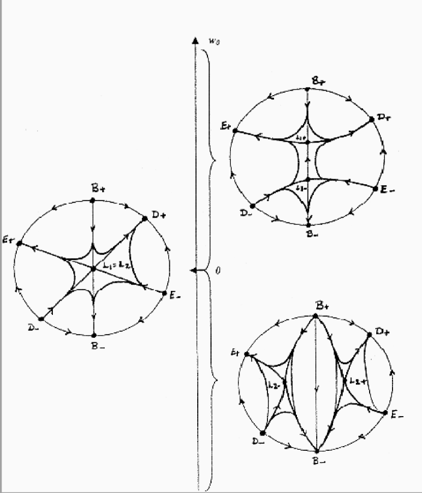
Figure 1: Phase portrait of the Poincare transformation of system (4.14)- (4.15): The case $w_{0}<0$ corresponds to spherically symmetric solutions, $w_{0}=0$ to plane symmetric solutions, and $w_{0}>0$ to hyperbolically symmetric solutions. The vertical direction represents the parameter space $w_{0}\in\Re$, where $w_{0}=0$ is the bifurcation value for the system.

A bifurcation diagram, including all the phase portraits for each range of the parameter $w_{0}$ is given in Figure 1. As can be seen by these phase portraits all generic asymptotic behavior (to the past and the future) is located on the infinite boundary. The exact solutions for each of these singular points (which are asymptotic states to past or future or are intermediate states) will be examined in section 5.

4.2 Subcase: $x_{4}=0$ - plane symmetry

The invariant set $x_{4}=0$ contains a subset of the asymptotic solutions for the system (4.1)-(4.4). As can be seen from equations (2.2) and (3.19), solutions which have $w$ identically zero comprise the set of plane symmetric solutions.

In this case, the system of ODEs (4.1)-(4.4) reduces to:

$$\dot{x_{1}} = x_{1}(x_{2}+x_{3})\ ,$$ (4.19)

$$\dot{x_{2}} = x_{2}(1+x_{3}-3x_{1}-x_{2})\ ,$$ (4.20)

$$\dot{x_{3}} = x_{1}^{2}+x_{3}(x_{1}+x_{2}-x_{3})\ .$$ (4.21)

The co-ordinate planes $x_{1}=0$ and $x_{2}=0$ are each invariant sets for this system, as are the sets $x_{1}+2x_{3}=0$ and $x_{1}=x_{3}$.

The finite singular points in this case are given by $Q_{1}$, $Q_{2}$, $Q_{3}$ and $L_{1}=L_{2}$. The local dynamics of each is determined by considering the sign of the eigenvalues of the Jacobian (see Table 1) restricted to this set $x_{4}=0$; i.e, those eigenvalues whose associated eigenvectors have the form $(c_{1},c_{2},c_{3},0)$. The points $Q_{1}$-$Q_{3}$ are saddles in this three-dimensional set. The point $L=L_{1}=L_{2}$ is non-hyperbolic. Center manifold theory [13] allows the point to be analyzed. The many invariant sets which include this point greatly simplify the analysis, and it is a straightforward matter to show that in the two dimensions which define the coordinate plane $x_{2}=0$ the point is a saddle and in the third direction it is a saddle-node. The infinite singular points (not including $C_{\pm}$) are given in Table 2. The dynamics on the infinite boundary is represented by Figures 2 and 3 (see [11] for details).

Before considering the global dynamics in this three-dimensional system, we shall consider the dynamics as restricted to the invariant planes. Each of these planes will divide the phase space further, allowing for a simplification in the analysis when considering the entire space. Note that the $x_{2}=0$ invariant set has been completely analyzed in the previous section. The dynamics are represented by the case $w_{0}=0$ in Figure 1. Therefore, we need only consider the planes $x_{1}=0$, $x_{1}+2x_{3}=0$ and $x_{1}=x_{3}$.

Invariant Set: $x_{1}=0$

In the invariant set $x_{1}=0$, the system (4.19)-(4.21) reduces to:

$$\dot{x_{2}} = x_{2}(1+x_{3}-x_{2})\ ,$$ (4.22)

$$\dot{x_{3}} = x_{3}(x_{2}-x_{3})\ ,$$ (4.23)

and represents the vacuum solutions in the full 4-dimensional system. This system gives rise to dynamics in the $x_{2}$ - $x_{3}$ plane. The finite singular points are given by $L_{1}=L_{2}=(0,0)$ and $Q_{1}=(1,0)$. Local analysis shows that the point $(1,0)$ is a saddle point and the point $(0,0)$ is non-hyperbolic, saddle-node in nature (determined through the use of center manifold theory). Therefore, no stable asymptotic behavior is located in the finite part of the phase space and all asymptotically stable solutions in this subcase are located on the infinite boundary. The complete phase portrait, as compactified by the Poincare transformation, is given in Figure 4.

Invariant Set: $x_{1}+2x_{3}=0$

In the invariant set $x_{1}+2x_{3}=0$, the system (4.19)-(4.21) reduces to:

$$\dot{x_{2}} = x_{2}(1+3x_{3}-x_{2}),$$ (4.24)

$$\dot{x_{3}} = x_{3}(x_{3}+x_{2}).$$ (4.25)

As a result the dynamics is located in a two-dimensional plane. The finite singular points are given by $Q_{1}=(1,0)$, $Q_{3}=(1/8,-1/8)$ and $L_{1}=L_{2}=(0,0)$. Local analysis determines that the point $(1,0)$ is a saddle, $(1/8,-1/8)$ a spiraling sink and $(0,0)$ a saddle-node (determined through the use of center manifold theory). The phase portrait for this case, as compactified by the Poincare transformation, is given in Figure 5. In this case the fluid is also physically self-similar.

Invariant Set: $x_{1}=x_{3}$

In the invariant set $x_{1}=x_{3}$, the system (4.19)-(4.21) reduces to:

$$\dot{x_{1}} = x_{1}(x_{1}+x_{2}),$$ (4.26)

$$\dot{x_{2}} = x_{2}(1-x_{2}-2x_{1}).$$ (4.27)

As a result the dynamics are located in a two-dimensional plane. The finite singular points are given by $L_{1}=L_{2}=(0,0)$, $Q_{1}=(0,1)$ and $Q_{2}=(1,-1)$. Local analysis determines that the points $(1,0)$ and $(1,-1)$ are saddles whereas $(0,0)$ is a saddle-node (determined through the use of center manifold theory). The phase portrait for this case, as compactified by the Poincare transformation, is given in Figure 6.

Global dynamics

The global dynamics can be determined through an investigation of the direction fields making use of the monotonicity principle [14]. To simplify the global analysis, consider the full three-dimensional phase space divided into 16 invariant regions and labelled $U_{i}$ so that $U_{13}$ corresponds to the set $x_{2}=0$, $U_{14}$ the set $x_{1}=0$, $U_{15}$ the set $x_{1}+2x_{3}=0$ and $U_{16}$ the set $x_{1}=x_{3}$. In each of the remaining 12 regions of space a monotonic function has been identified. These regions, and their corresponding monotonic functions, are given in Table 3. Note that the totality of the sets $U_{i}$, $i=1..16$ provides a decomposition of the complete phase space. As such, since each region is invariant under the system (4.19)-(4.21), the existence of strictly monotonic functions in the regions $U_{1}$ - $U_{14}$ ensures that the only possible asymptotic solutions are located on the boundaries (either finite or infinite). The finite boundaries are the sets $U_{13}-U_{16}$, or subsets thereof. As a result the global dynamics has been completely determined by the previous investigations. The only possible asymptotic states are, therefore, the singular points located at finite and infinite values. Furthermore, in the full four dimensional space the only possible asymptotic states are those singular points which are sinks or sources; namely the sinks $A_{+}$, $B_{-}$ and $D_{+}$ and the sources $A_{-}$, $B_{+}$, and $D_{-}$.

4.3 The case $x_{4}=\pm\infty$

¿From table 2 we see that the only solutions characterized by $x_{4}\rightarrow\pm\infty$ correspond to the points $C_{\pm}$, found by compactifying the phase space using a Poincare transformation. This point is ’non-hyperbolic’ in all four directions. To determine the exact nature of the local behavior of these points we consider the system (4.1)-(4.4) under the following change of coordinates:

$$Y_{1}=\frac{x_{1}}{x_{4}},\quad Y_{2}=\frac{x_{2}}{x_{4}},\quad Y_{3}=\frac{x_{3}}{x_{4}},\quad\mbox{and}\quad Y_{4}=\frac{1}{x_{4}},$$ (4.28)

and a ”time” variable that is defined by $f^{\prime}=Y_{4}\dot{f}$. The singular points of interest (namely $C_{\pm}$) are now located at the origin of the new coordinate system. In these new coordinates, the system (4.1)-(4.4) becomes:

$$Y_{1}^{\prime} = Y_{1}(Y_{3}-Y_{2})$$ (4.29)

$$Y_{2}^{\prime} = Y_{2}(Y_{4}+Y_{3}-3Y_{1}-3Y_{2})$$ (4.30)

$$Y_{3}^{\prime} = Y_{4}+Y_{1}^{2}+Y_{1}Y_{3}-Y_{2}Y_{3}-Y_{3}^{2}$$ (4.31)

$$Y_{4}^{\prime} = -2Y_{2}Y_{4}.$$ (4.32)

The singular points of interest (namely $C_{\pm}$) are now located at $(0,0,0,0)$. There are two invariant lines, namely $Y_{1}=Y_{3}=Y_{4}=0$ and $Y_{1}=Y_{2}=Y_{4}=0$. Each of these lines corresponds to an eigenvector of the flow for the system (4.29)-(4.32), and on each of these lines the flow is monotonic decreasing. The dynamics in a third direction can then be determined by considering the two-dimensional set $Y_{2}=Y_{4}=0$, i.e.:

$$Y_{1}^{\prime} = Y_{1}Y_{3}$$ (4.33)

$$Y_{3}^{\prime} = Y_{1}^{2}-Y_{3}^{2}+Y_{1}Y_{3}.$$ (4.34)

In this case $Y_{1}=Y_{3}$ and $Y_{1}=-2Y_{3}$ are invariant sets (and, again, eigenvectors of the flow). On each of these sets the derivatives are strictly positive or strictly negative, indicating that this point is a saddle-node.

Therefore in three of the four directions (of the full phase space) through the singular points $C_{\pm}$ the derivative does not change sign, and in the fourth direction there is no motion (as this direction is normal to the sheets of invariant planes described in the previous section). This point is, therefore, a higher-dimensional saddle-node.

5 Description of asymptotic solutions

In the qualitative analysis of the previous section, the asymptotic states of the governing system were described as singular points of the autonomous system of ODEs. The existence of other types of stable structures was ruled out by the existence of monotonic functions. While some of the singular points being described are not structurally stable in all 4-dimensions, there are invariant regions in which they do act as attractors (either to the past or the future); in addition, these points act as intermediate attractors (repellors) for large classes of solutions. Each of the physical solutions described by these singular points will now be given, restricting attention to those solutions which satisfy the weak and dominant energy conditions. In the case of infinite kinematic self-similarity, two of the boundaries of the regions which satisfy the energy conditions are, in fact, invariant sets; therefore we need only consider the solutions which lie in the regions $x_{1}\geq 0$ and $x_{4}+2x_{1}x_{3}+x_{1}^{2}\leq 0$. For the invariant set $x_{1}=0$, one has $\mu+p=0$ corresponding to a cosmological constant or vacuum if, in addition, $x_{4}=0$.

5.1 Finite singular point asymptotic states

$Q_{1}=(0,1,0,0)$ is a vacuum solution corresponding to Minkowski space-time. $Q_{2}=(1,-1,1,0)$ does not satisfy the energy conditions since $\mu-p<0$. $L_{1}=(0,0,\beta,\beta^{2})$, if $\beta\neq 0$, then $\mu+p=0$ and $\mu<0$ violating again the energy conditions. The remaining singular points are:

• $Q_{3}=(1/4,1/8,-1/8,0)$

  In this case the metric is plane symmetric

  $$ds^{2}=-\left({r\over t}\right)^{1/4}dt^{2}+{b^{2}\over r^{2}}\left({t\over r}\right)^{3/4}dr^{2}+\left({t\over r}\right)^{1/2}(d\theta^{2}+\theta^{2}d\phi^{2})\ ,$$ (5.1)

  where $b$ is a constant. The energy density and pressure are given by

  $$\mu=p={1\over 4t^{2}}\left({t\over r}\right)^{1/4}\ .$$ (5.2)

  The fluid is physically self-similar and it represents the only stiff-matter solution (i.e., $\mu=p$) in the plane symmetric case.

• $L_{2}=(\sigma,0,0,-\sigma^{2})$

  The case $\sigma=0$ (i.e., the intersection of $L_{1}$ and $L_{2}$) corresponds to Minkowski space-time. Otherwise, the metric is spherically symmetric

  $$ds^{2}=-dt^{2}+{s_{0}^{2}\sigma^{2}\over r^{2}}\left({t\over r}\right)^{2\sigma}dr^{2}+s_{0}^{2}\left({t\over r}\right)^{2\sigma}(d\theta^{2}+sin^{2}\theta d\phi^{2})\ ,$$ (5.3)

  where $s_{0}$ and $\sigma$ are constants. The energy density and pressure are

  $$\mu={3\sigma^{2}\over t^{2}}\ ,\quad p={-3\sigma^{2}+2\sigma\over t^{2}}\ .$$ (5.4)

  In this case the fluid is physically self-similar and satisfies the energy conditions for $\sigma\geq 1/3$. The case $\sigma=1/3$ corresponds to stiff-matter and $\sigma=2/3$ to dust.

5.2 Infinite singular point asymptotic states

The infinite singular points are displayed in Table 2. $A_{\pm}$, $B_{\pm}$ and $F_{\pm}$ correspond to vacuum solutions. They asymptote respectively to the following line elements:

$$ds^{2}(A)=-dt^{2}+{b^{2}\over r^{2}}\left[\ln\left({t\over r}\right)+c\right]^{2}dr^{2}+d\theta^{2}+\theta^{2}d\phi^{2}\ ,\quad{\rm for}\quad\ln\left({t\over r}\right)+c\rightarrow 0\ ,$$ (5.5)

$$ds^{2}(B)=-\left[\ln\left({t\over r}\right)+c\right]^{2}dt^{2}+{b^{2}\over r^{2}}dr^{2}+d\theta^{2}+\theta^{2}d\phi^{2}\ ,\quad{\rm for}\quad\ln\left({t\over r}\right)+c\rightarrow 0\ ,$$ (5.6)

$$ds^{2}(F)=-\exp\left[c\left({t\over r}\right)^{1/2}\right]dt^{2}+{b^{2}t\over r^{3}}\exp\left[c\left({t\over r}\right)^{1/2}\right]dr^{2}+d\theta^{2}+\theta^{2}d\phi^{2}\ ,\quad{\rm for}\quad{t\over r}\rightarrow\infty\ ,$$ (5.7)

where $b$ and $c$ are integration constants.

The singular points $C_{+}$, $D_{\pm}$, $E_{+}$, $G_{+}$, and $H_{\pm}$ do not satisfy energy conditions. Physical solutions (i.e., perfect fluid solutions satisfying the energy conditions) do not asymptote to these infinite singular points since they lie in different invariant regions of the phase space. The remaining singular points are:

• $C_{-}$: The metric is given by

  $$ds^{2}=-dt^{2}+{(\dot{S})^{2}\over r^{2}}dr^{2}+S^{2}(d\theta^{2}+sin^{2}\theta d\phi^{2})\ ,$$ (5.8)

  where

  $$S=s_{0}\left({t\over r}\right)^{1/3}\left[\ln\left({t\over r}\right)+c\right]^{2/3}\ ,\quad{\rm for}\quad\ln\left({t\over r}\right)+c\rightarrow 0\ ,$$ (5.9)

  $s_{0}$ and $c$ are constants. The matter quantities are

  $$\mu={1\over 3t^{2}}\left[1+{4\over\ln\left(t/r\right)+c}\right]\ ,\qquad p={1\over 3t^{2}}\ .$$ (5.10)

  The fluid in this case is physically self-similar.

• $E_{-}$: The metric is plane symmetric

  $$ds^{2}=-{1\over S}dt^{2}+{b^{2}\over r^{2}}S^{2}dr^{2}+S^{2}(d\theta^{2}+\theta^{2}d\phi^{2})\ ,$$ (5.11)

  where $S=[\ln(t/r)+c]^{2}$, for $\ln(t/r)+c\rightarrow 0$, $b$ and $c$ are constants. The matter variables are given by

  $$\mu={12\over t^{2}}\ ,\qquad\mu+p={4\over t^{2}}\left[\ln\left({t\over r}\right)+c\right]\ .$$ (5.12)

  Again the fluid is physically self-similar.

• $G_{-}$: In this final case the metric is plane symmetric given by:

  $$ds^{2}=-{1\over S}dt^{2}+{b^{2}\over r^{2}S}dr^{2}+S^{2}(d\theta^{2}+\theta^{2}d\phi^{2})\ ,$$ (5.13)

  where $S=[\ln(t/r)+c]^{1/2}$, for $\ln(t/r)+c\rightarrow 0$, $b$ and $c$ are constants.

  Notice that this line element is not a solution of the system (4.1)-(4.4). It is just the asymptotic solution when $\ln(t/r)+c\rightarrow 0$. For this reason we do not write the matter variables. All perfect fluid solutions approaching this singular point will tend to be physical self-similar. They will satisfy the energy conditions depending on the direction from which they are approaching this point. $G_{-}$ lies exactly in the boundary of a region in which the energy conditions are satisfied.

In all the solutions here presented, $t$, $r$ and $\theta$ have been rescaled in order to absorb as many integrating constants as possible.

6 Special Cases

Having completed the qualitative analysis and identified the possible asymptotic states, it is useful to note that in several of the invariant sets considered in the previous sections the system can be integrated completely so that the solutions can be written out explicitly. These particular sets are considered here.

6.1 The invariant set $x_{2}=0$

All of the exact solutions in this case can, in fact, be determined as the system (4.14)-(4.15) can be integrated completely. If $x_{1}=0$, the remaining equation yields $\dot{x}_{3}=w_{0}-x_{3}^{2}$. But in this case $\mu+p=0$ and perfect fluid solutions are excluded. For $x_{1}\neq 0$ we have that

$$x_{3}={\dot{x}_{1}\over x_{1}}\ ,$$ (6.1)

and equation (4.15) becomes

$$\ddot{x}_{1}=x_{1}(w_{0}+x_{1}^{2}+\dot{x}_{1})\ ,$$ (6.2)

that can be rewritten as

$$(2\dot{x}_{1}+x_{1}^{2})\dot{}=2x_{1}(2\dot{x}_{1}+x_{1}^{2}+w_{0})\ ,$$ (6.3)

or

$$(\dot{x}_{1}-x_{1}^{2})\dot{}=x_{1}(-\dot{x}_{1}+x_{1}^{2}+w_{0})\ .$$ (6.4)

The case $\dot{x}_{1}=0$ and $x_{1}\neq 0$ implies $w_{0}+x_{1}^{2}=0$ and corresponds to the fixed points $L_{2}$. Apart from this case the following possibilities arise.

Case: $2\dot{x}_{1}+x_{1}^{2}+w_{0}=0$.

Notice that all the solutions correspond to the intersection of the invariants sets $I_{2}$ and $I_{4}$. The different solutions depend on the value of $w_{0}$. They are:

• $w_{0}=0$: $x_{1}=2/\chi$, where $\chi\equiv\ln(t/r)+c$. The metric can be written as

  $$ds^{2}=-{1\over\chi^{2}}dt^{2}+{b^{2}\chi^{4}\over r^{2}}dr^{2}+\chi^{4}(d\theta^{2}+\theta^{2}d\phi^{2})\ ,$$ (6.5)

  where $b$ and $c$ are constants.

• $w_{0}=+\beta^{2}$: $x_{1}=-\beta\tan(\beta\chi/2)$ and

  $$ds^{2}=-[\tan(\beta\chi/2)]^{2}dt^{2}+s_{0}^{2}[\cos(\beta\chi/2)]^{4}\left({\beta^{2}\over r^{2}}dr^{2}+d\theta^{2}+\sinh^{2}\theta d\phi^{2}\right)\ ,$$ (6.6)

  $s_{0}$ being a constant.

• $w_{0}=-\beta^{2}$: Two possibilities arise, $x_{1}=\beta\tanh(\beta\chi/2)$ or $x_{1}=\beta\coth(\beta\chi/2)$. The line elements are

  $$ds^{2}=-[\tanh(\beta\chi/2)]^{2}dt^{2}+s_{0}^{2}[\cosh(\beta\chi/2)]^{4}\left({\beta^{2}\over r^{2}}dr^{2}+d\theta^{2}+\sin^{2}\theta d\phi^{2}\right)\ ,$$ (6.7)

  and

  $$ds^{2}=-[\coth(\beta\chi/2)]^{2}dt^{2}+s_{0}^{2}[\sinh(\beta\chi/2)]^{4}\left({\beta^{2}\over r^{2}}dr^{2}+d\theta^{2}+\sin^{2}\theta d\phi^{2}\right)\ ,$$ (6.8)

  respectively.

All of these solutions satisfy the energy conditions only over some limited regions of the manifold.

Case: $-\dot{x}_{1}+x_{1}^{2}+w_{0}=0$.

Different solutions appear again depending on $w_{0}$. They correspond to the intersection of the invariant sets $I_{2}$ and $I_{5}$.

• $w_{0}=0$: $x_{1}=-1/\chi$, and the metric can be written as

  $$ds^{2}={1\over\chi^{2}}\left(-dt^{2}+{b^{2}\over r^{2}}dr^{2}+d\theta^{2}+\theta^{2}d\phi^{2}\right)\ .$$ (6.9)

  The metric is conformally flat.

• $w_{0}=+\beta^{2}$: $x_{1}=\beta\tan(\beta\chi)$,

  $$ds^{2}=-[\tan(\beta\chi)]^{2}dt^{2}+{s_{0}^{2}\over[\cos(\beta\chi)]^{2}}\left({\beta^{2}\over r^{2}}dr^{2}+d\theta^{2}+\sinh^{2}\theta d\phi^{2}\right)\ .$$ (6.10)

• $w_{0}=-\beta^{2}$: $x_{1}=-\beta\tanh(\beta\chi)$ or $x_{1}=-\beta\coth(\beta\chi)$.

  $$ds^{2}=-[\tanh(\beta\chi)]^{2}dt^{2}+{s_{0}^{2}\over[\cosh(\beta\chi)]^{2}}\left({\beta^{2}\over r^{2}}dr^{2}+d\theta^{2}+\sin^{2}\theta d\phi^{2}\right)\ ,$$ (6.11)

  and

  $$ds^{2}=-[\coth(\beta\chi)]^{2}dt^{2}+{s_{0}^{2}\over[\sinh(\beta\chi)]^{2}}\left({\beta^{2}\over r^{2}}dr^{2}+d\theta^{2}+\sin^{2}\theta d\phi^{2}\right)\ ,$$ (6.12)

  respectively.

In all cases $b$, $\beta$ and $s_{0}$ are constants.

Case: $2\dot{x}_{1}+x_{1}^{2}+w_{0}\neq 0$ and $-\dot{x}_{1}+x_{1}^{2}+w_{0}\neq 0$.

Equations (6.3) and (6.4) can be integrated to yield

$$2\dot{x}_{1}+x_{1}^{2}+w_{0}=3\sigma S^{2}\ ,$$ (6.13)

and

$$-\dot{x}_{1}+x_{1}^{2}+w_{0}={3\lambda\over 2}{1\over S}\ ,$$ (6.14)

where $\sigma$ and $\lambda$ are arbitrary non-null constants. Comparing equations (6.13) and (6.14) we find

$$x_{1}^{2}=\sigma S^{2}+{\lambda\over S}-w_{0}\ .$$ (6.15)

Hence, once $S$ is know, all the other metric functions can be calculated. ¿From (6.1) we get

$$e^{2\Phi}=x_{1}^{2}\ ,$$ (6.16)

and also we have

$$e^{2\Psi}=b^{2}S^{2}\ ,$$ (6.17)

where $b^{2}=-w_{0}k$ for $k\neq 0$ and any arbitrary constant for $k=0$. Then substituting $x_{1}=\dot{S}/S$ in equation (6.15) one gets

$${\dot{S}\over\sqrt{\sigma S^{4}-w_{0}S^{2}+\lambda S}}=\pm 1\ .$$ (6.18)

This is the only equation that needs to be integrated. Thus, this case $x_{2}=0$ is completely solved up to quadratures.

6.2 The case $x_{3}=0$ (and $\dot{x}_{3}=0$)

This case is of particular interest since all the solutions belong to the intersection of the invariant sets $I_{4}$ and $I_{5}$ and therefore they are physically self-similar. They represent the geodesic solutions for the system; i.e., these solutions have zero acceleration. Since the governing equations impose the condition $x_{4}=-x_{1}^{2}$, there can be no hyperbolically symmetric solutions in this case. The plane symmetric case is the special case $x_{1}=0$ and this corresponds to vacuum solutions. Their metric is given by

$$ds^{2}=-dt^{2}+\left(1+a{t\over r}\right)^{2}{b^{2}\over r^{2}}dr^{2}+d\theta^{2}+\theta^{2}d\phi^{2}\ ,$$ (6.19)

where $a$ and $b$ are constants.

All the other solution will exhibit spherical symmetry, and the metric can be written as

$$ds^{2}=-dt^{2}+\frac{\dot{S}^{2}}{r^{2}}dr^{2}+S^{2}(d\theta^{2}+\sin^{2}\theta d\phi^{2})\ .$$ (6.20)

The governing equations reduce to

$$\dot{x}_{1} = x_{1}x_{2}\ ,$$ (6.21)

$$\dot{x}_{2} = x_{2}(1-3x_{1}-x_{2})\ ,$$ (6.22)

and substituting $x_{2}$ from (6.21) into equation (6.22), we obtain

$$\ddot{x}_{1}=-3x_{1}\dot{x}_{1}+\dot{x}_{1}\ .$$ (6.23)

A first integral this equation is

$$\dot{x}_{1}=-{3\over 2}\left[\left(x_{1}-{1\over 3}\right)^{2}+n\right]\ ,$$ (6.24)

where $n$ is an arbitrary constant. The special case $\dot{x}_{1}=0$ corresponds to the curve $L_{2}$ of singular points. The other solutions depend on the different value of the constant $n$ and they are

• $n=0$: $x_{1}=1/3+1/\chi$; $S=s_{0}(t/r)^{1/3}\chi^{2/3}$, where now $\chi\equiv(3/2)(\ln(t/r)+c)$, $c$ being a constant.

• $n=\beta^{2}$: $x_{1}=1/3-\beta\tan(\beta\chi)$; $S=s_{0}(t/r)^{1/3}[\cos(\beta\chi)]^{2/3}$.

• $n=-\beta^{2}$: $x_{1}=1/3+\beta\tanh(\beta\chi)$; $S=s_{0}(t/r)^{1/3}[\cosh(\beta\chi)]^{2/3}$,

  or $x_{1}=1/3+\beta\coth(\beta\chi)$; $S=s_{0}(t/r)^{1/3}[\sinh(\beta\chi)]^{2/3}$.

The solutions satisfy the energy conditions if $x_{1}>0$ and $x_{1}\geq 1/3+3n$.

7 Physical self-similarity

As was stated in the introduction, the cases of physical and geometric self-similarity are not necessarily equivalent when considering KSS spacetimes. Perfect fluid solutions will necessarily be physically self-similar if they satisfy $x_{4}+2x_{1}x_{3}+x_{1}^{2}=0$, and hence lie in the invariant set $I_{4}$. In this case the system (4.1)-(4.4) reduces to the three-dimensional system of autonomous ODEs:

$$\dot{x_{1}} = x_{1}(x_{2}+x_{3})\ ,$$ (7.1)

$$\dot{x_{2}} = x_{2}(1-3x_{1}-x_{2}+x_{3})\ ,$$ (7.2)

$$\dot{x_{3}} = x_{3}(-x_{1}+x_{2}-x_{3})\ .$$ (7.3)

Through the use of monotonic functions it can be shown that all of the asymptotic behavior in this class of solutions is described by solutions in one (or more) of the invariant sets $x_{1}=0$, $x_{2}=0$, $x_{3}=0$ or $x_{1}+2x_{3}=0$, all of which have been previously discussed. The case $x_{1}=0$ corresponds to the vacuum case, and the exact solutions for the cases $x_{2}=0$ and $x_{3}=0$ can be found in section 6.1 and 6.2, respectively.

In the case of physical self-similarity, perfect fluid solutions have a barotropic equation of state if, in addition, they satisfy

$$2x_{2}+3x_{1}=c_{1}\ ,$$ (7.4)

where $c_{1}$ is an arbitrary constant. In Table 4, we summarize all the possible barotropic, physical self-similar solutions.

8 Discussion

To summarize, we have studied perfect fluid (spherically, plane and hyperbolically symmetric) space-times admitting a kinematic self-similarity of infinite type. We have restricted our attention to the case in which the kinematic self-similar vector field commutes with all of the the Killing vectors. Three different cases arise depending on the orientation of the fluid flow relative to the kinematic self-similar vector. The interesting general case is the ‘tilted’ one in which the four-velocity is neither parallel nor orthogonal to the self-similar vector field. In this case, we have shown that the governing equations reduce to a four-dimensional autonomous system of ODEs. The qualitative properties of the system have been fully studied. In particular, through an extensive use of monotonic functions, we have shown that all asymptotic solutions in this infinite class of kinematic self-similarity are necessarily located at singular points (either at finite or infinite values of the dependent variables) which are classified in Tables 1 and 2.

Most of these singular points are saddle points in the full phase space, although there are invariant regions in which they do act as sinks or sources, thereby acting as attractors (or repellors) for classes of solutions. The only global sinks and sources are located on the infinite boundary, summarized in Table 5. Hence, in general solutions asymptote to one of those represented by the points A₊, B₊ or D_- in the past and one of those represented by the points A_-, B_- or D₊ in the future.

The physical solutions described by these singular points are given in the cases in which the weak and dominant energy conditions are satisfied. The class of solutions which are also physically self-similar are again important in this analysis. We show that in all cases in which the energy conditions are satisfied the asymptotic behavior is necessarily physical self-similar and the space-time is plane or spherically symmetric. This result coincides with the results of Benoit and Coley [10], which studied the case of spherical symmetry with finite kinematic self-similarity. This again shows the relevance of the physical self-similar models.

In some special cases, e.g., the invariant set $x_{2}=0$, and the geodesic case, corresponding to the case $x_{3}=0$, the four-dimensional autonomous system of ODEs can be integrated completely. All the exact solutions have been found in these cases (see Sections 6 and 7). In the geodesic case, the solutions are again physically self-similar. These exact solutions serve as illustrations of the more general qualitative results previously discussed. Finally, we have also found all of the physical self-similar solutions that admit a barotropic equation of state. The results are summarized in Table 4.

Table 1: Finite Singular Points for equations (4.1)-(4.4). The local analysis for each singular point will be discussed in the subsequent sections, according to their classification. ${\bf Q}_{1,2,3}$ are isolated singular points and ${\bf L}_{1}$ and ${\bf L}_{2}$ are curves of non-isolated singular points (one-dimension equilibrium sets). Note that the curves ${\bf L}_{1}$ and ${\bf L_{2}}$ intersect at the point $(0,0,0,0)$, which is a saddle-node. $\beta$ and $\sigma$ are constants.

	$(x_{1},x_{2},x_{3},x_{4})$	Eigenvalue - Eigenvector Pairs		Classification
${\bf Q}_{1}$	$(0,1,0,0)$	$1$	$(0,1,2,0)$	Saddle
		$1$	$(1,0,3,0)$
		$-1$	$(0,1,0,0)$
		$2$	$(0,1,3,3)$
${\bf Q}_{2}$	$(1,-1,1,0)$	$-3$	$(5,-6,-9,0)$	Saddle
		$-2$	$(-4,5,3,7)$
		$1+\sqrt{2}$	$(1,\sqrt{2},1,0)$
		$1-\sqrt{2}$	$(1,-\sqrt{2},1,0)$
${\bf Q}_{3}$	$(\frac{1}{4},\frac{1}{8},\frac{-1}{8},0)$	$3/4$	$(1,0,3,0)$	Saddle
		$1/4$	$(-2,1,-3,2)$
		$-(1-\sqrt{7}i)/8$	$(-2,-\sqrt{7}i,1,0)$
		$-(1+\sqrt{7}i)/8$	$(-2,\sqrt{7}i,1,0)$
${\bf L}_{1}$	$(0,0,\beta,\beta^{2})$	$\beta$	$(3,0,1,0)$	Curve of Saddle Points
		$1+\beta$	$(0,1+\beta,\beta,2\beta^{2})$
		$-2\beta$	$(0,0,1,0)$
		$0$	$(0,0,1,2\beta)$
${\bf L}_{2}$	$(\sigma,0,0,-\sigma^{2})$	$-\sigma$	$(-1,0,1,0)$	Curve of Saddle Points
		$2\sigma$	$(1,0,2,0)$
		$1-3\sigma$	$(\sigma,-2\sigma,0,-3\sigma)$
		$0$	$(1,0,0,-2\sigma)$

Table 2: Classification of the Infinite Singular Points of the Poincare transformed system (4.1)-(4.4)]. The exact solutions for each of these points are described in section 5.2.

	$(X_{1},X_{2},X_{3},X_{4})$	Eigenvalue - Eigenvector Pairs		Classification
A±	$(0,\pm 1,0,0)$	$\pm 2$	$(1,0,0,0)$
		$\pm 2$	$(0,1,0,0)$	A+ : Source
		$\pm 2$	$(0,0,1,0)$
		$\pm 3$	$(0,0,0,1)$	A- : Sink
B±	$(0,0,\pm 1,0)$	$\pm 2$	$(1,0,0,0)$
		$\pm 2$	$(0,1,0,0)$	B+ : Source
		$\pm 2$	$(0,0,1,0)$
		$\pm 1$	$(0,0,0,1)$	B- : Sink
C±	$(0,0,0,\pm 1)$	$0$	$(1,0,0,0)$
		$0$	$(0,1,0,0)$	Saddle-Node
		$0$	$(0,0,1,0)$
		$0$	$(0,0,0,1)$
D±	$\frac{\sqrt{2}}{2}(\pm 1,0,\pm 1,0)$	$\mp\sqrt{2}$	$(1,0,1,0)$
		$\mp\frac{\sqrt{2}}{2}$	$(0,0,0,1)$	D+ : Sink
		$\mp\frac{3\sqrt{2}}{2}$	$(-1,0,1,0)$
		$\mp\frac{3\sqrt{2}}{2}$	$(0,1,0,0)$	D- : Source
E±	$\frac{\sqrt{5}}{5}(\mp 2,0,\pm 1,0)$	$\pm\frac{6\sqrt{5}}{5}$	$(0,1,0,0)$
		$\mp\frac{6\sqrt{5}}{5}$	$(1,0,2,0)$	Saddle
		$\mp\frac{\sqrt{5}}{5}$	$(0,0,0,1)$
		$\mp\frac{2\sqrt{5}}{5}$	$(-2,0,1,0)$
F±	$\frac{\sqrt{2}}{2}(0,\pm 1,\pm 1,0)$	$\mp\sqrt{2}$	$(0,-1,1,0)$
		$\pm\sqrt{2}$	$(2,-1,1,0)$	Saddle
		$\pm\sqrt{2}$	$(0,0,0,1)$
		$0$	$(0,1,1,0)$
G±	$\frac{\sqrt{14}}{14}(\mp 2,\pm 3,\pm 1,0)$	$\pm\frac{\sqrt{14}}{7}$	$(0,0,0,1)$
		$\mp\frac{4\sqrt{14}}{7}$	$(2,-3,-1,0)$	Saddle
		$\mp\frac{3\sqrt{14}}{7}$	$(1,0,2,0)$
		$\mp\frac{3\sqrt{14}}{7}$	$(0,1,-3,0)$
H±	$\frac{\sqrt{17}}{17}(\pm 1,\mp 3/2,\pm 1,0)$	$\mp\frac{27\sqrt{17}}{136}$	$(134,-201,257,0)$
		$\mp\frac{\sqrt{17}}{34}$	$(2,-3,2,0)$	Saddle
		$\pm\frac{21\sqrt{17}}{136}$	$(63,118,63,0)$
		$\mp\frac{23\sqrt{17}}{136}$	$(0,0,0,1)$

Table 3: Invariant regions of the space $(x_{1},x_{2},x_{3})$ for the system (4.19)-(4.21) with corresponding monotonic functions. Note that the sets $U_{13}-U_{16}$ are not included here as they are two-dimensional invariant sets and their complete dynamics have been summarized in the phase portraits: Figures 2-6 .

s Label	Definition of Region	Monotonic
		Function
$U_{1}$	$\{(x_{1},x_{2},x_{3})|x_{1},x_{2},x_{3}>0\}$	$x_{1}$ strictly increasing
$U_{2}$	$\{(x_{1},x_{2},x_{3})|x_{1},x_{2}>0,x_{1}+2x_{3}>0\}$	$x_{1}+2x_{3}$ strictly increasing
$U_{3}$	$\{(x_{1},x_{2},x_{3})|x_{1},x_{2}>0,x_{1}+2x_{3}<0\}$	$x_{1}+2x_{3}$ strictly decreasing
$U_{4}$	$\{(x_{1},x_{2},x_{3})|x_{1}<0,x_{2}>0,x_{1}-x_{3}<0\}$	$x_{1}-x_{3}$ strictly decreasing
$U_{3}$	$\{(x_{1},x_{2},x_{3})|x_{1}<0,x_{2}>0,x_{1}-x_{3}>0\}$	$x_{1}-x_{3}$ strictly increasing
$U_{6}$	$\{(x_{1},x_{2},x_{3})|x_{1}<0,x_{2},x_{3}>0\}$	$x_{1}$ strictly decreasing
$U_{7}$	$\{(x_{1},x_{2},x_{3})|x_{1}>0,x_{2}<0,x_{1}-x_{3}<0\}$	$x_{1}-x_{3}$ strictly increasing
$U_{8}$	$\{(x_{1},x_{2},x_{3})|x_{1}>0,x_{2}<0,x_{1}-x_{3}>0\}$	$x_{1}-x_{3}$ strictly decreasing
$U_{9}$	$\{(x_{1},x_{2},x_{3})|x_{1}>0,x_{2}<0,x_{3}<0\}$	$x_{1}-x_{3}$ strictly decreasing
$U_{10}$	$\{(x_{1},x_{2},x_{3})|x_{1},x_{2},x_{3}<0\}$	$x_{1}$ strictly increasing
$U_{11}$	$\{(x_{1},x_{2},x_{3})|x_{1},x_{2}<0,x_{1}+2x_{3}<0\}$	$x_{1}+2x_{3}$ strictly increasing
$U_{12}$	$\{(x_{1},x_{2},x_{3})|x_{1},x_{2}<0,x_{1}+2x_{3}>0\}$	$x_{1}+2x_{3}$ strictly decreasing

Table 4: Infinite kinematic self-similar perfect fluid solutions admitting a barotropic equation of state. The weak and dominant energy conditions are always satisfied, except in the last case in which $c_{1}\geq 1$.

Case	Solution	Remarks
$c_{1}=0$	$x_{1}=0$, $x_{2}=0$, $x_{3}=[\ln(t/r)+c]^{-1}$, $x_{4}=0$	vacuum
$c_{1}=1$	$x_{1}=1/4$, $x_{2}=1/8$, $x_{3}=-1/8$, $x_{4}=0$	$Q_{3}$: stiff-matter
$c_{1}=1$	$x_{1}=1/3$, $x_{2}=0$, $x_{3}=0$, $x_{4}=-1/9$	$L_{2}$: stiff-matter
$c_{1}=2$	$x_{1}=0$, $x_{2}=1$, $x_{3}=0$, $x_{4}=0$	$Q_{1}$: vacuum
$c_{1}=2$	$x_{1}=2/3$, $x_{2}=0$, $x_{3}=0$, $x_{4}=-4/9$	$L_{2}$: dust
$c_{1}=2$	$x_{3}=0$, $x_{4}=-x_{1}^{2}$, $x_{2}=1-3x_{1}/2$
	see case $x_{3}=0$, with $\beta=1/3$, $n=-1/9$	dust
$c_{1}\neq 0,1,2$	$x_{1}=c_{1}/3$, $x_{2}=0$, $x_{3}=0$, $x_{4}=-c_{1}^{2}/9$	$L_{2}$

Table 5: Summary of the global asymptotic behaviour.

Singular Point	Nature of the Singular Point	Physical Characteristics of Solutions
A+	Source: Global attractor to the past	Geodesic, vacuum solution;
		physically self-similar
A-	Sink: Global attractor to the future	Geodesic, vacuum solution;
		physically self-similar
B+	Source: Global attractor to the past	Vacuum solution;
		physically self-similar
B-	Sink: Global attractor to the future	Vacuum solution;
		physically self-similar
D+	Sink: Global attractor to the future	Energy conditions not satisfied
D-	Source: Global attractor to the past	Energy conditions not satisfied

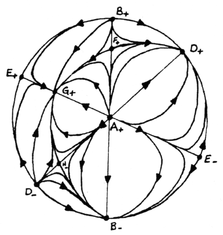
Figure 2: Dynamics on the infinite boundary for the plane symmetric solutions: for the Poincare transformed space. Top hemisphere; i.e. $X_{2}>0$

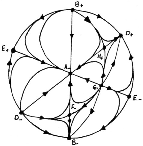
Figure 3: Dynamics on the infinite boundary for the plane symmetric solutions: for the Poincare transformed system. Bottom hemisphere; i.e. $X_{2}<0$

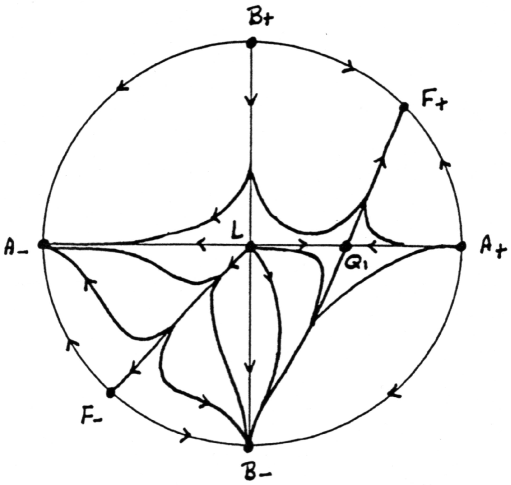
Figure 4: Phase portrait of the Poincare transformed system (4.22)- (4.23): plane symmetric solutions restricted to the invariant set $x_{1}=0$. The phase space is $X_{2}$ vs. $X_{3}$.

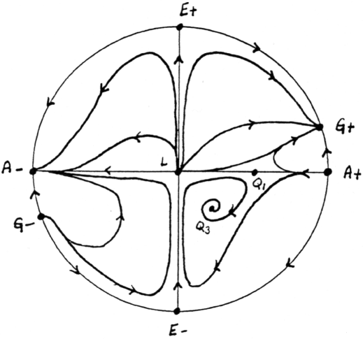
Figure 5: Phase portrait of the Poincare transformed system (4.24)- (4.25): plane symmetric solutions restricted to the invariant set $x_{1}+2x_{3}=0$. The phase space is $X_{2}$ vs. $X_{3}$.

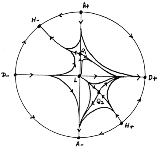
Figure 6: Phase portrait of the Poincare transformed system (4.26)- (4.27): plane symmetric solutions restricted to the invariant set $x_{1}=x_{3}$. The phase space is $X_{1}$ vs. $X_{2}$.

References

- [1] L.I. Sedov, Similarity and Dimensional Methods in Mechanics, Academic Press, New York (1959).
- [2] G.E. Barenblatt and Ya. B. Zeldovich, 1972, Ann. Rev. Fluid Mech., 4, 285.
- [3] M.E. Cahill and A H. Taub, 1971, Comm. Math. Phys. 21, 1.
- [4] D.M. Eardley, 1974, Comm. Math. Phys. 37, 287.
- [5] D.M. Eardley, 1974, Phys. Rev. Lett. 33, 442.
- [6] B. Carter and R.N. Henriksen, 1989, Annales de Physique, Paris Suppl. no 6, 14, 47.
- [7] B. Carter and R.N. Henriksen, 1991, J. Math. Phys. 32, 2580.
- [8] A. A. Coley, 1997, Class. Quant. Grav. 14, 87.
- [9] A. M. Sintes, 1998, Class. Quant. Grav. 15, 3689.
- [10] P. M. Benoit and A. A. Coley, 1998, Class. Quant. Grav. 15, 2397.
- [11] P. M. Benoit, 1999, PhD Thesis, Dalhousie University
- [12] A. A. Coley and B. O. J. Tupper, 1994, Class. Quant. Grav. 11, 2553.
- [13] J. Guckenheimer and P. Holmes, 1983, Nonlinear Oscillations, Dynamical Systems, and Bifurcations (Wiley)
- [14] V. G. LeBlanc, D. Kerr, and J. Wainwright, 1995, Class. Quant. Grav, 12, 513
- [15] D. Lynden-Bell and J. P. S. Lemos, 1988, Mon. Not. R. Ast. Soc. 233, 197.
- [16] R. Maartens, D. P. Mason and M. Tsamparlis, 1986, J. Math. Phys. 27, 2987.