Discrete Symmetries in Translation Invariant Cosmological Models

Abstract

In this paper we investigate a class of $(d+1)$ dimensional cosmological models with a cosmological constant possessing an ${\mathbb{R}}^{d}$ simply transitive symmetry group and show that it can be written in a form that manifests the effect of a permutation symmetry. We investigate the solution orbifold and calculate the probability of a certain number of dimensions that will expand or contract. We use this to calculate the probabilities up to dimension $d=5$.

1 Introduction

The effect of symmetries of differential equations on their solutions were first truly recognized by the Norwegian mathematician Sophus Lie more than hundred years ago. Lie made considerable progress on the effect of so-called transformation groups on the solutions of differential equations. A simple symmetry principle can yield many interesting properties of the solutions to the equations of motion for a physical system. In gauge theories the complete Lagrangian can be deduced by a requirement that it should be invariant under a certain symmetry. In cosmology there have been many studies written of the so-called Bianchi universes. Bianchi universes are spatially homogeneous cosmological models that can be classified according to Bianchi’s classification of the 3-dimensional Lie algebras. They are numbered $I-IX$ and are in general anisotropic.

The object of this paper is to investigate a certain family of spatially homogeneous cosmological models. We will investigate $(d+1)$ dimensional space-times with a simply transitive symmetry group ${\mathbb{R}}^{d}$. The metric for these models can be written

$$ds^{2}=-N(t)^{2}dt^{2}+\sum_{i=1}^{d}a_{i}(t)^{2}(dx^{i})^{2}$$ (1)

For $d=3$ this is called the Bianchi type I model. In this paper we will focus on another symmetry that these space-times possess. We note that the metric 1 is also invariant under the discrete symmetry group $S_{d}$, the symmetric group, or the permutation group of $d$ elements. The labelling of each coordinate $x^{i}$ , $i=1,...,d$ is somewhat artificial and can be permuted to any other sequence, thus the mapping $(x^{1},...,x^{i},...x^{d})\longmapsto(x^{k_{1}},...,x^{k_{i}},...x^{k_{d}})$ where $(k_{1},...,k_{i},...k_{d})$ is any permutation of $(1,...,i,...,d)$ is a symmetry transformation. This will be the main observation of this paper.

Let us introduce the notion of a regular $(d-1)$-simplex, $\sigma_{d-1}$. It is the generalization of an equilateral triangle to any dimension. We embed $\sigma_{d-1}$ in Euclidean $(d-1)$ space, $\sigma_{d-1}\subset{\mathbb{R}}^{d-1}$ and write ${\bf n}_{i}$ to denote the position of the $i$th vertex relative to the center of mass frame. For simplicity, if we write ${\bf n}_{i}$ as a column vector, we define a $(d-1)\times d$ matrix ${\bf Q}$ by

$${\bf Q}=[{\bf n}_{1},...,{\bf n}_{d}]=[(n^{a}_{i})]$$ (2)

By regularity of $\sigma_{d-1}$, we get the following two relations

$$\sum_{i=1}^{d}{\bf n}_{i} = 0$$ (3)

$$|{\bf n}_{i}-{\bf n}_{j}| = \ell,~{}i\neq j$$ (4)

We can now state the theorem which we shall prove in the next section:

Theorem:

The general solution for the line element (1) of the vacuum Einstein field equations $R_{\mu\nu}-\frac{1}{2}Rg_{\mu\nu}+\Lambda g_{\mu\nu}=0$ in $(d+1)$ dimensions is

$$ds^{2}=-\frac{dt^{2}}{\left(1-\frac{d}{2(d-1)}\Lambda t^{2}\right)^{2}}+\frac{t^{\frac{2}{d}}}{\left(1-\frac{d}{2(d-1)}\Lambda t^{2}\right)^{\frac{2}{d}}}d\tilde{s}^{2}$$ (5)

where

$$d\tilde{s}^{2}=\sum_{i=1}^{d}t^{\frac{2(d-1)}{d}n^{a}_{i}}(dx^{i})^{2}$$ (6)

and $n^{a}_{i}$, $i=1,...,d$ correspond to a regular $(d-1)$-simplex inscribed in the unit $(d-2)$ sphere, or de Sitter’s solution with flat spatial sections.

De Sitter’s solution is, as we shall see, completely disconnected from the other solutions and we will in the further disregard this solution. This theorem has been proven for $d=2$ and $d=3$ in previous works [2, 3]. The $d=2$ case is illustrated in figure 1. The $d=3$ case which is usually called the Bianchi type I solution, is proved in [3] and illustrated in figure 2. We have also illustrated the case $d=4$ in figure 3 which is a regular tetrahedron inscribed in the unit 2-sphere.

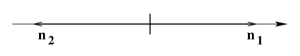
Figure 1: The $d=2$ case.

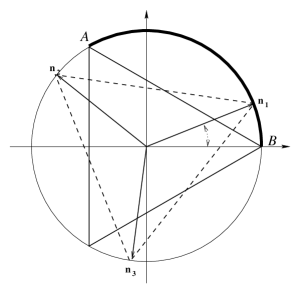
Figure 2: The $d=3$ case. The bold arc $AB$ is a double covering of the solution orbifold in this case. The point represented by the angle $\frac{\pi}{3}$ will be a reflection point under the orbifold identification.

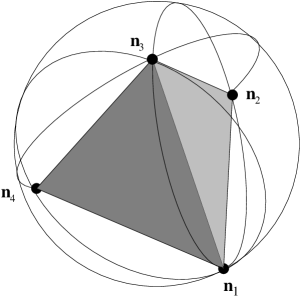
Figure 3: The $d=4$ case.

The case $d=1$ is trivial and a 0-simplex is simply a point. But since the ${(-1)}$-sphere is somewhat poorly defined, we can just say that $\sigma_{0}={0}$. This results in the Milne line element for $\Lambda=0$:

$$ds^{2}=-dt^{2}+t^{2}dx^{2}$$

We will exclude the $d=1$ case in what follows.

2 Proof

For simplicity we will consider a vanishing cosmological constant. The results can easily be expanded to a non-zero cosmological constant by similar methods as in the paper [3].

With $\Lambda=0$ one can easily derive the solutions of eq. (1). The solutions are usually written:

$$ds^{2}=-dt^{2}+\sum_{i}t^{2p_{i}}(dx^{i})^{2}$$ (7)

where $\sum_{i}p_{i}=1$ and $\sum_{i}p_{i}^{2}=1$.

By using of the permutation group $S_{d}$ under which the solution space must be invariant, we will show that these two descriptions are equivalent. We first inscribe the regular simplex $\sigma_{d-1}$ in the unit sphere $S^{d-2}$. Since ${\bf n}_{i}\in S^{d-2}$, we have $\sum_{a}(n_{i}^{a})^{2}=1$. By evaluating the sums $\sum_{i,j}\sum_{a}(n^{a}_{i}-n_{j}^{a})^{2}$ and $\sum_{a}(n_{i}^{a}-n_{j}^{a})^{2}$ in two different ways we can obtain the following useful relations:

$$\ell = \sqrt{\frac{2d}{d-1}}$$ (8)

$${\bf n}_{i}\cdot{\bf n}_{j}|_{i\neq j} = -\frac{1}{d-1}$$ (9)

We notice that the symmetry group of a regular $(d-1)$-simplex Sym($\sigma_{d-1}$) (including orientation-reversing operations) is isomorphic to $S_{d}$. More specifically, each element of the group Sym($\sigma_{d-1}$) is a permutation of the vertices ${\bf n}_{i}$. Thus we immediately have two different representations of the permutation group $S_{d}$. The first is $d\times d$ matrices $\Gamma(g)\in O(d)$ ($g\in S_{d}$). These matrices represent the permutation of the vectors ${\bf n}_{i}$. The second representation consists of $(d-1)\times(d-1)$ matrices $\gamma(g)\in O(d-1)$ and the matrices $\gamma(g)$ are for a fixed orientation of $\sigma_{d-1}\subset{\mathbb{R}}^{d-1}$ the $O(d-1)$-rotations of $\sigma_{d-1}$ that map $\sigma_{d-1}$ onto itself. Hence we have the following relation:

$$\gamma(g){\bf Q}={\bf Q}\Gamma(g)$$ (10)

Notice that along the diagonal of the matrix ${\bf N}\equiv{\bf Q}{\bf Q}^{T}$ we have elements of the type $\sum_{i}(n_{i}^{a})^{2}$. We further note that

$$\gamma(g){\bf N}\gamma(g)^{T}=\gamma(g){\bf Q}{\bf Q}^{T}\gamma(g)^{T}={\bf Q}\Gamma(g)\Gamma(g)^{T}{\bf Q}^{T}={\bf Q}{\bf Q}^{T}={\bf N}$$ (11)

for all $g\in S_{d}$. On the left side of this equation the diagonal elements are permuted compared to the right side. Since the above equation holds for all $g\in S_{d}$ we must have

$$\sum_{i}(n_{i}^{a})^{2}=\sum_{i}(n_{i}^{b})^{2},~{}\forall a,b$$ (12)

We now obtain

$$\sum_{i}(n^{a}_{i})^{2}=\frac{1}{d-1}\sum_{a}\sum_{i}(n^{a}_{i})^{2}=\frac{1}{d-1}\sum_{i}\sum_{a}(n^{a}_{i})^{2}=\frac{1}{d-1}\sum_{i}1=\frac{d}{d-1}$$ (13)

Now we show that $\sum_{i}(\frac{1}{d}+\frac{d-1}{d}n^{a}_{i})$ and $\sum_{i}(\frac{1}{d}+\frac{d-1}{d}n^{a}_{i})^{2}$ both sum to 1. The first sum is

$$\sum_{i}\left(\frac{1}{d}+\frac{d-1}{d}n^{a}_{i}\right) = \frac{1}{d}\sum_{i}1+\frac{d-1}{d}\sum_{i}n^{a}_{i}$$ (14)

$$= 1;$$ (15)

while the second sum is

$$\sum_{i}\left(\frac{1}{d}+\frac{d-1}{d}n^{a}_{i}\right)^{2} = \frac{1}{d^{2}}\sum_{i}\left[1+2(d-1)n^{a}_{i}+(d-1)^{2}(n^{a}_{i})^{2}\right]$$ (16)

$$= \frac{1}{d^{2}}[d+(d-1)d]$$ (17)

$$= 1$$ (18)

Thus we have shown that equations (5) and (6) are solutions of the Einstein field equation as the theorem claims. But does the theorem span the whole set of solutions that can be written $\sum_{i}p_{i}=1$ and $\sum_{i}p_{i}^{2}=1$? The equation $\sum_{i}p_{i}^{2}=1$ describes a $(d-1)$ sphere and $\sum_{i}p_{i}=1$ a $(d-1)$ dimensional hyperplane. The intersection of these two spaces is a $(d-2)$ sphere $S^{d-2}$. From the other perspective, the group $G=O(d-1)$ acts transitively on the sphere $S^{d-2}$ and thus is the group of all orientations of the regular simplex $\sigma_{d-1}$. The solution space of the metrics given in the theorem is the projection of the vertices of $\sigma_{d-1}$. This projection onto (for instance) the 1st axis is invariant under the isotropy group of $(1,0,...,0)\in S^{d-2}$ which is $O(d-2)$. Thus the solution space of the metric of the theorem has the universal cover $O(d-1)/O(d-2)\cong S^{d-2}$ . Thus the two descriptions have solution spaces which equal the same compact space. Hence they are equivalent.

We would also emphasize that the solution space is the orbifold $S^{d-2}/S_{d}$, i.e. we identify points on the $(d-2)$-sphere under the action of the symmetric group. This action is not free: there are fixed points under this action. If $y\in S^{d-2}$ is fixed under a subgroup $G\subset S_{d}$ then we say that $y$ is a $G$ fixed point. $G$ will be isomorphic to $S_{h}$ for $h\leq d$ or a direct product of these, and if $y$ is a $S_{h_{1}}\times...\times S_{h_{m}}$ fixed point then $y$ will correspond to a $SO(h_{1})\times...\times SO(h_{m})$ symmetric spacetime. Hence these fixed points are actually spacetimes with higher symmetry than originally assumed.

The inversion map

It is quite clear that the mapping: ${\mathcal{R}}:{\bf Q}\longmapsto-{\bf Q}$ maps a solution ${\bf Q}$ onto an other solution $-{\bf Q}$. Geometrically this is the reflection of the simplex through the origin. This is not one of the symmetry operations of the regular simplex, thus $-{\bf Q}\neq{\bf Q}$.

Let us simultaneously consider the mapping:

$${\mathfrak{I}}:t\longmapsto\frac{1}{\omega^{2}t}$$ (19)

for $\Lambda\neq 0$ and $\omega^{2}=\frac{d}{2(d-1)}|\Lambda|$. The map ${\mathfrak{I}}$ maps expanding solutions onto contracting solutions. For positive $\Lambda$ this means that the contracting branch, where $\omega t>1$, is mapped onto the expanding branch $\omega t<1$. We note that the composition of the maps ${\mathcal{R}}$ and ${\mathfrak{I}}$ is almost the identity map (or an isometry). The resulting metric can be written in the same way as the original metric except that the spatial coordinates have been rescaled. The resulting map

$$dx^{i}\longmapsto\omega^{\frac{2(d-1)}{d}n^{a}_{i}}dx^{i}$$ (20)

is just a rescaling of the space coordinates. It also interesting to note when this mapping is an isometry. This always happens if $\omega=1$. If $\omega\neq 1$ then either $n^{a}_{i}=0$ or the spatial coordinates $x^{i}$ have to be infinite in range. This has to be true for all $i$.

Even though the map ${\mathfrak{I}}$ is not defined for $\omega=0$ the map $\mathcal{R}$ is, and we can say that the map $\mathcal{R}$ is a duality relation between contracting and expanding solutions.

3 A special class of solutions: flat-fibered FRW solutions

In the previous section we have given a simple relation fulfilled by any $d$-dimensional, translation invariant solution. In this section we will look at a subclass of solutions that describe a flat FRW universe with flat fibres, and we will again assume that $\Lambda\neq 0$.

In the previous sections we have used a time gauge in which each of the scale factors $a_{i}(t)\equiv\sqrt{g_{ii}}$ are (up to a proportionality factor) given by

$$a_{i}(t)=\frac{t^{\frac{1}{d}(1+(d-1)n_{i}^{a})}}{(1-\lambda t^{2})^{\frac{1}{d}}}$$ (21)

This time gauge will be called the Kasner time gauge. Notice that the spatially $d$-volume varies as

$$V(t)\propto\prod_{i=1}^{d}a_{i}(t)=\frac{t}{1-\lambda t^{2}}$$ (22)

We define the universal time gauge as

$$\eta=\int_{0}^{t}\frac{d\tau}{1-\lambda\tau^{2}}$$ (23)

The scale factors in the universal time gauge are ($\omega=\sqrt{|\lambda|}$)

$$a_{i}(\eta)=\begin{cases}(\sinh\omega\eta)^{\frac{1}{d}(1+(d-1)n_{i}^{a})}(\cosh\omega\eta)^{\frac{1}{d}(1-(d-1)n_{i}^{a})},&\Lambda>0\\ \eta^{\frac{1}{d}(1+(d-1)n_{i}^{a})},&\Lambda=0\\ (\sin\omega\eta)^{\frac{1}{d}(1+(d-1)n_{i}^{a})}(\cos\omega\eta)^{\frac{1}{d}(1-(d-1)n_{i}^{a})},&\Lambda<0\end{cases}$$ (24)

while the spatially $d$-volume is

$$V(\eta)\propto\prod_{i=1}^{d}a_{i}(\eta)=\begin{cases}(\sinh\omega\eta)(\cosh\omega\eta),&\Lambda>0\\ \eta,&\Lambda=0\\ (\sin\omega\eta)(\cos\omega\eta),&\Lambda<0\end{cases}$$ (25)

Let us define the following two vectors for positive integers $n,m$ where $n+m=d$:

$$\xi_{n}=\frac{1}{n}\sum_{i=1}^{n}{\bf n}_{i}$$ (26)

and

$$\xi_{m}=\frac{1}{m}\sum_{i=1+n}^{m+n}{\bf n}_{i}$$ (27)

Their norms are easily calculated by the use of $|{\bf n}_{i}|=1$ and relation 9:

$$|\xi_{n}|^{2}=\frac{m}{n(d-1)}$$ (28)

$$|\xi_{m}|^{2}=\frac{n}{m(d-1)}$$ (29)

Assuming that $n_{i}^{a}=|\xi_{n}|$ for $1\leq i\leq n$ and $n_{i}^{a}=-|\xi_{m}|$ for $1+n\leq i\leq n+m=d$, it follows that $\sum_{i}(n^{a}_{i})^{2}=\frac{d}{d-1}$ and $\sum_{i}n^{a}_{i}=0$. A interesting point is that the $n^{a}_{i}$’s are bounded by

$$(d-1)^{2}\geq(d-1)|n^{a}_{i}|\geq 1$$ (30)

Thus we will have

$$\dot{a}_{i}\geq 0 ,\text{for}~{}1\leq i\leq n$$ (31)

independent of the value of the cosmological constant (and whether $a_{i}$ is expressed in the universal time gauge or in the Kasner gauge). Thus we have that one flat section is always expanding, even if the cosmological constant is negative!(see figures 4 and 5.)

Figure 4: The typical expansion of a scale factor in the expanding part of the metric in the Kasner time gauge. For $\Lambda>0$ the scale factors will go to infinity as $t\longrightarrow\omega^{-1}$ because of the denominator in (21). The time $t=\omega^{-1}$ represents the isotropic limit.

Figure 5: The typical expansion of a scale factor in the expanding part of the metric in the universal time gauge. Note that as the $d$-volume collapses in the final singularity, the expanding part will grow to infinite size for $\Lambda<0$.

An example from String Theory

All the five consistent string theories demand a (9+1) dimensional spacetime. One usually compactifies 6 spatial dimensions to a Calabi-Yau (CY) manifold[7]. If $d\Sigma_{m}^{2}$ is the $m$-dimensional Euclidean metric we will assume therefore that the metric takes the form

$$ds^{2}=-N^{2}dt^{2}+a^{2}d\Sigma_{3}^{2}+a_{CY}^{2}d\Sigma_{6}^{2}.$$

This metric describes a flat FRW metric with a 6-dimensional fibering. We now take a 8-simplex and inscribe it in the unit 8-sphere, assuming that $n_{1}^{1}=n_{2}^{1}=n_{3}^{1}$ and $n_{4}^{1}=...=n_{9}^{1}$. We then find:

$$|\xi_{3}|=\frac{1}{2}$$ (32)

Similarly, we have

$$|\xi_{6}|=\frac{1}{4}.$$ (33)

If we set $n_{i}^{1}=|\xi_{3}|$ and $n_{j}^{1}=-|\xi_{6}|$ for $i=1,2,3$ and $j=4,...,9$ the $n_{k}^{1}$ fulfill all the necessary relations. Thus we get the solution:

$$ds^{2}=-\frac{dt^{2}}{\left(1-\frac{9}{16}\Lambda t^{2}\right)^{2}}+\frac{1}{\left(1-\frac{9}{16}\Lambda t^{2}\right)^{\frac{2}{9}}}\left(t^{\frac{10}{9}}d\Sigma_{3}^{2}+t^{-\frac{2}{9}}d\Sigma_{6}^{2}\right)$$ (34)

Let us now assume $\Lambda=0$. If we compactify $d\Sigma_{6}^{2}$ to be a compact CY-manifold and compactify $d\Sigma_{3}^{2}$ we note that while the volume of $d\Sigma_{3}^{2}$ is expanding, Vol$(d\Sigma_{3}^{2})\propto t^{\frac{5}{3}}$, the volume of the CY is contracting, Vol$(d\Sigma_{6}^{2})\propto t^{-\frac{2}{3}}$. Thus even in this simple classical model we obtain a mechanism that yields a possibility that while the physical 3-space expands, the CY-manifold shrinks to arbitrarily small size. If we had included a cosmological constant the relative sizes between the 3-space and the CY would become constant after a while. Thus if this universe undergoes inflation, the CY manifold would be fixed to a small size compared to the other 3 spatial dimensions.

The other solution where the spacetime metric possesses the same symmetries as the above metric is found by using the reflection map $\mathcal{R}$. The result is simply:

$$ds^{2}=-\frac{dt^{2}}{\left(1-\frac{9}{16}\Lambda t^{2}\right)^{2}}+\frac{1}{\left(1-\frac{9}{16}\Lambda t^{2}\right)^{\frac{2}{9}}}\left(t^{-\frac{2}{3}}d\Sigma_{3}^{2}+t^{\frac{2}{3}}d\Sigma_{6}^{2}\right)$$ (35)

Here we have an opposite behaviour, the volume of $d\Sigma_{3}^{2}$ is contracting as Vol$(d\Sigma_{3}^{2})\propto t^{-1}$, and the volume of the CY is expanding Vol$(d\Sigma_{6}^{2})\propto t^{2}$. We note a peculiar thing, the effect on the FRW part of the “reflected” solution of the model has a different behaviour than the original one. This is directly related to the fact that the dimensionalities of the FRW part and CY part are not equal.

4 Universes with matter and investigations of the solution orbifolds

So far we have discussed vacuum solutions only with a cosmological constant. We have investigated some special classes of solutions but have not actually discussed whether these solutions are probable or not. In the following we will introduce matter into the universe, a special kind of matter that possesses similar symmetries as that of the space itself. Let us look at scalar fields with a Lagrangian:

$${\mathcal{L}}_{M}=-\frac{1}{2}\sqrt{-g}\left[\sum_{c=1}^{\delta}\partial_{\mu}\phi_{c}\partial^{\mu}\phi_{c}+V(\phi_{c})\right]$$ (36)

where $\delta$ is the number of scalar fields. To sustain spatial homogeneity in our models the scalar fields have to be position independent i.e. $\phi_{c}(t)$. Thus if $V(\phi_{c})$ is constant the scalar fields will possess a ${\mathbb{R}}^{\delta}$ symmetry. These scalar fields can play the role of additional dimensions in these models. With the aid of the Lagrangian this is quite easy to see. The gravitational Einstein-Hilbert action $S_{G}=\int_{M}\sqrt{-g}(R-2\Lambda)d^{4}x+\int_{\partial M}2Kd^{3}x$ turns out to be:

$$S_{G}=\int dt\left[\frac{e^{d\alpha}}{N}\left(-d(d-1)\dot{\alpha}^{2}+\sum_{i=1}^{d}\dot{\beta}_{i}^{2}\right)-2N\Lambda e^{d\alpha}\right]$$ (37)

where $a_{i}\equiv\exp(\alpha+\beta_{i})$ and $\sum_{i=1}^{d}{\beta_{i}}=0$. Since the $\beta_{i}$’s are not independent we will instead introduce a set of variables $X^{a},~{}a=1,...,d-1$. We choose a simplex as described in earlier sections with the corresponding matrix ${\bf Q}$, we can write both $(\beta_{i})$ and $(X^{a})$ as column vectors, with

$$\beta=(d-1){\bf Q}^{T}X$$ (38)

This is a linear homeomorphism and the image is exactly the set of allowed $\beta_{i}$’s. This can be seen if one notes that the matrix ${\bf N}={\bf Q}{\bf Q}^{T}$ is proportional to the identity matrix (due to Schur’s lemma). Then, we have

$$\sum_{i=1}^{d}\dot{\beta}_{i}^{2}=d(d-1)\sum_{a=1}^{d-1}(\dot{X}^{a})^{2}$$ (39)

Thus the action for a $d$-dimensional universe with $\delta$ massless scalar fields is simply

$$S=\int dt\left[\frac{e^{d\alpha}}{2N}\left(-2d(d-1)\dot{\alpha}^{2}+2d(d-1)\sum_{i=1}^{d-1}(\dot{X}^{a})^{2}+\sum_{c=1}^{\delta}\dot{\phi}_{c}^{2}\right)-2N\Lambda e^{d\alpha}\right]$$ (40)

Hence up to a trivial rescaling of the $\phi_{c}$, the $X^{a}$ and the $\phi_{c}$ appear in the action on equal footing. The action cannot see the difference between the scalar field and the $X^{a}$ except in the global scaling of the volume factor $\alpha$.

The classical solutions can now be obtained. Choosing the Kasner time gauge $\exp(d\alpha)=tN$ the solutions are (up to a constant by addition):

$$X^{a} = \frac{1}{d}\eta^{a}\ln t$$ (41)

$$\phi_{c} = \sqrt{\frac{2(d-1)}{d}}\eta^{d-1+c}\ln t$$ (42)

$$\exp(d\alpha) = \frac{t}{1-\frac{d}{2(d-1)}\Lambda t^{2}}$$ (43)

Writing $\eta^{\mu},~{}\mu=1,...,d+\delta-1$ the $\eta^{\mu}$ will be coordinates on the unit $(d+\delta-2)$-sphere: $\sum_{\mu}(\eta^{\mu})^{2}=1$. The scalar fields behave just as the other variables $X^{a}$ and is in some sense compensating for the other dimensions that are not there! The scalar fields are reducing the sphere containing the simplex. If the sphere has zero radius the metric is a FRW metric with no anisotropy. All the $\eta^{\mu}$’s for $\mu=1,...,d-1$ have to be exactly zero and the result turns simply into the case where

$$d\tilde{s}^{2}=\sum_{i=1}^{d}(dx^{i})^{2}$$ (44)

However, this is an exceptional case. In the set of all configurations this set of FRW universes is of zero measure, but the set of configurations where all Kasner parameters are positive has non-zero measure.

As we have seen, the vacuum Bianchi type I solutions $(d=3)$ can be seen as the orbifold $S^{1}/S_{3}$. Since the order of $S_{3}$ is 6, which is usually written $|S_{3}|=6$, the solution orbifold can be seen as an arc of length $\frac{\pi}{3}$. The fixed points under the orbifold identification are the end points of this arc and represent universes with higher symmetry than originally assumed. In the $d=3$ case these points correspond to the two different $SO(2)$ symmetric spacetimes. An $SO(2)$ symmetric spacetime has zero measure. All the other vacuum solution cases will have 2 expanding ($e$) and 1 contracting ($c$) direction, i.e. $P(2e+1c)=1$ where $P$ is the probability. If we include a scalar field the situation changes to $S^{2}/S_{3}$. Now we assume that the probability of each solution is weighted by the natural geometry of the solution orbifold (which is spherical). The probabilities turn out to be

$$P(2e+1c) = \frac{3}{4}$$ (45)

$$P(3e) = \frac{1}{4}$$ (46)

The most probable scenario is still a universe with 2 expanding and 1 contracting solution but nevertheless there is a non-zero probability that there are 3 expanding directions.

The case $d=4$

Increasing the number of dimensions the complexity increases drastically. However the next step, the $d=4$ case, can also be illustrated easily.

Figure 6: The vacuum $d=4$ solution orbifold. The dotted line separates the $(2e+2c)$ solutions from the $(3e+1c)$ solutions.

The solution space of the Kasner coordinates can now be illustrated by a $(\frac{\pi}{2},\frac{\pi}{3},\frac{\pi}{3})$ spherical triangle on the 2-sphere $S^{2}$, see figure 6. Again, all the fixed points are on the boundary of this triangle and correspond to universes with higher symmetry than originally assumed. The $\frac{\pi}{2}$ vertex correspond to a universe with symmetry $SO(2)\times SO(2)$ and the other 2 vertices correspond to the two different $SO(3)$ symmetric spacetimes. The rest of the rim of the triangle represents different versions of $SO(2)$ symmetric spacetimes. But these spacetimes have measure zero as a set compared to the whole solution set.

In this case it is also interesting to calculate the various probabilities of different numbers of contracting and expanding directions. The result for the vacuum case is:

$$P(2e+2c) = \frac{1}{3}$$ (47)

$$P(3e+1c) = \frac{2}{3}$$ (48)

Now we see that the odds for a universe with 3 expanding directions are 2:1. Thus the most probable case is a universe with 3 expanding directions and 1 contracting one.

The case with 3 expanding directions will be even more probable if we include a scalar field. Then the solution space is that of a 3-sphere $S^{3}$ with certain identifications under the symmetric group $S_{4}$. Interestingly, using the orthogonal projection, we can map this space onto two solid balls, each ball corresponds to the North and South hemispheres of $S^{3}$. By suitable choice of coordinates, one ball is for positive scalar field, the other for negative. The characteristic solutions will now divide the space into different regions. Except for sets of measure zero, these regions will correspond to $(2e+2c)$, $(3e+1c)$ and $(4e)$ solutions. In the orthogonal projection model, the $(4e)$ regions will be two solid regular ideal tetrahedrons, one in each ball. However, using the pull-back metric from the projection of the sphere $S^{3}$, the metric in the two balls will be:

$$ds^{2}=\frac{dr^{2}}{1-r^{2}}+r^{2}(d\phi^{2}+\sin^{2}\phi d\theta^{2})$$ (49)

Finding the different probabilities will now be considerably more difficult but can be calculated numerically. The result is:

$$P(2e+2c) = 0.136$$ (50)

$$P(3e+1c) = 0.805$$ (51)

$$P(4e) = 0.059$$ (52)

Thus, there will be with an 80% chance that the universe (at least initially) has 3 expanding directions and 1 contracting. One dimension will automatically contract and be of arbitrary small size compared to the other ones. It is assumed that quantum gravity effects dominates when $t<t_{Pl}$ and one would naively believe that the wavefunction is evenly distributed over configuration space. In the region $t>>t_{Pl}$ collisionless particles counteract on the metric and make contracting directions unstable[8]. The contracting directions will eventually start to expand and the net effect is an evolution towards an isotropic universe.

The $d=5$ vacuum case is also calculated and some explanation of the calculation is made in the appendix. The results obtained are summarized in table 1.

	$d=3$ V	$d=3$ SF	$d=4$ V	$d=4$ SF	$d=5$ V
2e	1	$\frac{3}{4}$	$\frac{1}{3}$	0.136	0.257
3e	0	$\frac{1}{4}$	$\frac{2}{3}$	0.805	0.389
4e	-	-	0	0.059	0.355
5e	-	-	-	-	0

Table 1: Summary of the probability calculations done in this paper. The V stands for vacuum case, the SF for scalar field case.

5 Conclusion and Discussion

We have shown that the solutions of the general $(d+1)$ dimensional spacetime with a translational invariant metric can be written in different ways. The solution space of the model had the orbifold structure $S^{d-2}/S_{d}$ in the vacuum case and $S^{d-1}/S_{d}$ when a scalar field is present. We wrote the solutions as a $(d-1)$-plet under the permutation group which could be interpreted as the coordinates of the vertices of a regular $(d-1)$-simplex. This simplex possesses the same discrete symmetries as the model and gave a geometrical description of the solution space.

This representation of the solution space was useful for several reasons. As we saw in [3], we may have a continuous transition to an isotropic FRW universe by a reduction of the radius of the sphere in which the simplex $\sigma_{d-1}$ is inscribed. The symmetries of the solutions are manifest under this continuous transition. Another property of the ordinary Bianchi type I solutions is that there are particular solutions which appear to be special. These solutions play a very special role in the solution space: They are the fixed points under the orbifold identification of the sphere with respect to the symmetry group of the simplex which was isomorphic to the symmetric group $S_{d}$. These fixed points have the special property that they represent spacetimes that have a larger symmetry group than the original ${\mathbb{R}}^{d}$. Also, the type of the fixed point, (i.e. if it is a reflection fixed point or an $S_{3}$ fixed point) determined the symmetry of the resulting spacetime. In general, an $S_{n}$ fixed point would yield a $SO(n)$ symmetric spacetime and any product $S_{n}\times...\times S_{m}$ fixed point would yield a $SO(n)\times...\times SO(m)$ symmetric spacetime (in addition to translation symmetry). The set of solutions which is represented by ${\bf Q}$ does not have these special points. This is because the solution space of different ${\bf Q}$’s are $O(d-1)$ and the representation of the group $S_{d}$ acts freely and properly discontinuous on the manifold $O(d-1)$ by left (or right) multiplication. Thus the quotient $O(d-1)/S_{d}$ is a smooth manifold [5]. There are no special points.

We also obtained a cosmological solution which describes a (9+1) dimensional spacetime where 6 flat dimensions contract to arbitrarily small size, while 3 spatial dimensions expand to arbitrarily large size. However we emphasized that this is a special solution and the set of such solutions had only measure zero in the whole solution. By using this geometrical description we calculated various probabilities that certain configurations existed.

In this we paper have given a systematic approach to how such solution spaces “look like”. It would be interesting to finding out more of the properties in even higher dimensions than those investigated here. There may be a link between these solutions and the concept of chaos which is known to exist in certain of these spacetimes [9].

In the context of quantum cosmology these issues are indeed very interesting. As we have in this paper only considered classical probabilities under the assumption that all the points in the solution space were equally probable, it would be interesting to investigate whether the quantum calculations will yield the same results or whether more symmetric cases are favoured [10, 11].

Appendix

A $D$-simplex $\sigma_{D}\equiv[{\bf n}_{1},...,{\bf n}_{D+1}]$ (the order is irrelevant) can be parametrized in ${\mathbb{R}}^{m},~{}m\leq D$ by:

$$\sigma_{D}=\left\{{\bf x}\in{\mathbb{R}}^{m}|{\bf x}=\sum_{i=1}^{D+1}c_{i}{\bf n}_{i},c_{i}\geq 0,\sum_{i=1}^{D+1}c_{i}=1\right\}$$ (53)

A thing to note here is that a simplex is actually a whole set of simplices:

$$K=\left\{[{\bf n}_{1}],...,[{\bf n}_{D+1}],[{\bf n}_{1},{\bf n}_{2}],...,\sigma_{D+1}\right\}$$ (54)

In $K$ the number of $i$-simplices are $\frac{(D+1)!}{(D-i)!(i+1)!}$.

Let us consider a regular simplex with all its vertices on the unit sphere: $\sigma_{D}\subset{\mathbb{R}}^{D},~{}{\bf n}_{i}\in S^{D-1}$. The (covering) solution space of the vacuum case is now represented by the sphere $S^{D-1}$. Under the orthogonal projection the solution space of the models with one scalar field will be two such spheres $S^{D-1}$ but including their interior and with their boundaries identified. Thus homeomorphic to the $D$-sphere $S^{D}$. If we assume the ordinary round metric of the $D$-sphere, the metric under the orthogonal projection will be

$$ds^{2}=\frac{dr^{2}}{1-r^{2}}+r^{2}d\Omega_{D-1}^{2}$$ (55)

where $d\Omega_{D-1}^{2}$ is the ordinary round metric of the $(D-1)$ sphere. The advantage of this orthogonal projection of the single scalar field case is that if we do the projection in the scalar field direction the hyperspheres that represent Kasner indices with value zero become hyperplanes after the projection. The result is the “Euclidean” simplex inscribed in the sphere. The vacuum case can also be “dimensionally reduced” in a similar way. But now it is helpful to use the stereographic projection with respect to one of the vertices on the sphere. The stereographic projection is illustrated in figure 7. The “null” circles though this vertex will again become hyperplanes, the remaining “null” circle will be mapped onto a sphere, and the remaining vertices will lie on this sphere. Again, it appears as if we have a simplex inscribed in a sphere. However, the Euclidean metric has to replaced by the metric

$$ds^{2}=\frac{4}{(1+r^{2})^{2}}(dr^{2}+r^{2}d\Omega_{D-2}^{2})$$ (56)

The last vertex of the original simplex is at infinity.

Figure 7: The stereographic projection of the sphere.

These “null” spheres will divide the space into different open regions. Let us assume that we consider only one of the hemispheres in the scalar field case, their calculated volumes must then afterwards be multiplied by 2. To determine the type of region we are considering here are some rules (considering only vacuum case or one scalar field):

1. Each region will have a number of vertices $V>1$ connected to it.

2. If $E$ is the number of expanding dimensions and $C$ the number of contracting dimensions then $V=E$ and $d=D+1=E+C$.

3. The number of $V$-regions for $V\neq d$ are $\frac{d!}{(d-V)!V!}$.

4. The number of $V=d$ regions is 1 in the scalar field case and 0 in the vacuum case.

To calculate the various probabilities assuming each point is equally probable we have to calculate:

$$P(E+C)=\frac{\text{Vol}(E-regions)}{\text{Vol}(S^{D-1+\epsilon})}$$ (57)

where $\epsilon=1$ in the presence of a scalar field and 0 otherwise.

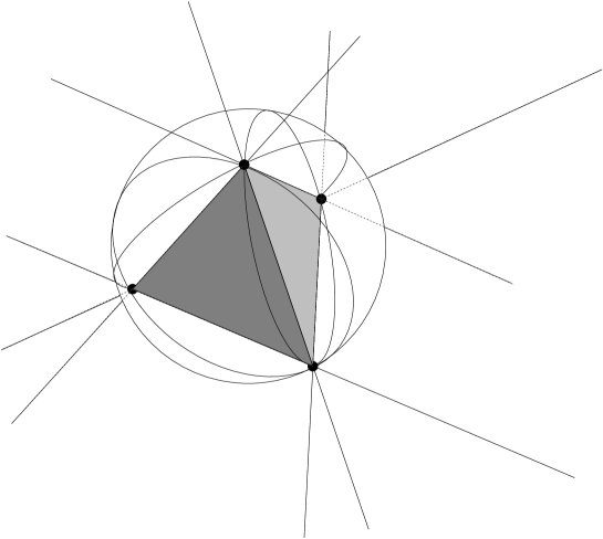
Figure 8: The vacuum $d=5$ case after a stereographic projection. Note that there is also a vertex at infinity.

Let us look at the vacuum $d=5$ case illustrated in figure 8. The volume of the 3-sphere is Vol$(S^{3})=2\pi^{2}$. The region inside the tetrahedron in the center has 4 vertices, thus corresponding to $(4e+1c)$ solutions. This tetrahedron can be parametrized and its volume can be computed using the round metric. Doing so, we obtain the volume:

$$\text{Vol}(Tetrahedron)=1.40$$ (58)

(with the aid of a computer). There are in all $\frac{5!}{1!4!}=5$ such regions, thus we have:

$$P(4e+1c)=\frac{5\text{Vol}(Tetrahedron)}{2\pi^{2}}=0.355$$ (59)

We can also calculate an upper bound for $P((d-1)e+1c)$ in the vacuum case for any dimension. We note that in the vacuum case the central $(d-2)$-simplex in the stereographic projection has a smaller volume than its Euclidean counterpart of the same “size”. This calculation yields the formula:

$$P((d-1)e+1c)<\frac{2^{d-3}d^{\frac{d}{2}}(d-1)^{\frac{d-1}{2}}\Gamma\left(\frac{d-1}{2}\right)}{(d-2)![(d-1)^{2}-1]^{\frac{d-2}{2}}\pi^{\frac{d-1}{2}}}$$ (60)

For $d<6$ this is actually larger than one, and is not very informative. But in the large $d$ limit the upper bound will go as $\propto d^{-\frac{d}{2}}$ which is much smaller than if we naively would have assumed that all the regions had equal size. In the latter case we would have got $\approx d\cdot 2^{-d}$.

References

- [1] M. Ryan and L. Shepley, Homogeneous Relativistic Cosmologies. Princeton University Press, (1975)
- [2] S. Carlip, Quantum Gravity in 2+1 Dimensions, Cambridge University Press, (1998)
- [3] S. Hervik, Class. Quantum Grav. 17, 2765 (2000)
- [4] M. Nakahara, Geometry, Topology and Physics, IoP Publishing (1990)
- [5] W.P. Thurston, Three-Dimensional Geometry and Topology, Volume 1, Princeton University Press (1997)
- [6] J. Polchinski, String Theory, Cambridge University Press, (1998)
- [7] B. Green, Lecture notes from TASI-96, hep-th/9702155
- [8] V.N. Lukash and A.A. Starobinskii, Sov. Phys. JETP 39, 742 (1974)
- [9] T. Damour and M. Henneaux, hep-th/0006171 (2000)
- [10] E.J. Copeland, J. Gray and P.M. Saffin, hep-th/0003244 (2000)
- [11] J. Gray and E.J. Copeland, hep-th/0102090 (2001)