Electromagnetic fields around black holes and Meissner effect

Abstract

The work on black holes immersed in external stationary magnetic fields is reviewed in both test-field approximation and within exact solutions. In particular we pay attention to the effect of the expulsion of the flux of external fields across charged and rotating black holes which are approaching extremal states. Recently this effect has been shown to occur for black hole solutions in string theory and Kaluza-Klein theory.

1 Introduction

Although much insight into the structure of external electromagnetic fields around black holes was obtained in 1970s and 1980s already, an interest in this theme continues being supported by the appearance of new motivations. To those coming from classical relativity belongs the “membrane paradigm” [1] – in the following (Section 4) we shall briefly discuss its validity for almost extreme black holes. Another “classical” issue is the behaviour of fields on the Cauchy (inner) horizons of charged or rotating holes [2]. Astrophysically, the discovery of microquasars in our Galaxy [3] makes the mechanism of the energy extraction from rotating black holes testable more directly than it has been possible with supermassive black holes in distant galactic nuclei. We refer to the contributions in these proceedings (and literature quoted therein) by M. Camenzind and R. Khanna and by B. Punsley (see also [4]) on the role of – still not properly understood – Blandford-Znajek and related mechanisms of electromagnetic extraction of rotational energy; Hyun Kyu Lee considers such processes to explain gamma ray bursts (see also [5]). In Section 5 exact spacetimes with black holes in strong fields will be considered (we shall also mention the possibility of the existence of a “cosmic supercollider” formed by a supermassive black hole surrounded by a superstrong magnetic field [6]).

Finally, new motivations have appeared with studies of black hole solutions in spacetimes with the dimensions either lower or higher than four within the framework of various “model” or “unified theories”. A useful survey of these “generalized” black holes, in fact of essentially all important developments in physics of black holes up to 1998 is contained in the new monograph by V. Frolov and I. Novikov [7]. In Section 6 we shall outline some new results on the expulsion of magnetic (or more general) gauge fields from extremal black holes in string theory.

Before mentioning these new developments we shall briefly review our earlier results on coupled perturbations of Reissner-Nordström black holes (Section 2) and on the fluxes of magnetic fields across black holes (Section 3).

2 Perturbations of charged black holes

The study of the perturbations of charged, non-rotating black holes can be motivated from several viewpoints: (i) the Reissner-Nordström solution is the simplest solution involving a limit - when the charge $Q$ and mass $M$ satisfy the condition of extremality $(Q^{2}=M^{2})$ - beyond which the horizon is absent; (ii) the holes’ interiors contain the Cauchy horizons where generic perturbations should imply instability; (iii) the electromagnetic perturbations are in general coupled with the gravitational perturbations. This leads to such intriguing effects as the conversion of gravitational waves into electromagnetic ones, or the appearance of closed magnetic field lines caused by “effective gravitational currents”; the coupling can also be used to study rigorously the motion of a black hole under an external, non-gravitational influence. Some of these effects will be discussed in the following.

The necessity of the coupling can easily be understood from the perturbed Einstein-Maxwell equations written symbolically in the form

$$\delta G=8\pi\delta T,$$ (1)

where the perturbed energy-momentum tensor, $\delta T\sim F^{(0)}\delta F$, is linear in perturbations because of the presence of the background Coulomb-type electric field $F^{(0)}\sim Q/r^{2}$. Hence, the left-hand side of (1), the perturbed Einstein tensor, is linear in metric perturbations $\delta g$ (and their derivatives). The perturbed Maxwell equations, $F_{\alpha\sigma}^{;\sigma}=4\pi j_{\alpha}$, turn out to read explicitly as follows [8]:

$$(\delta F_{\alpha\sigma})^{;\sigma}=4\pi\delta j_{\alpha}+(\delta j_{\alpha})_{grav.},$$ (2)

where the effective “gravitational current” is given by

$$\left(\delta j_{\alpha}\right)_{grav.}=F^{(0)}_{\alpha\rho;\sigma}h^{\rho\sigma}+F^{(0)\rho\sigma}h_{\alpha\rho;\sigma}+{{F^{(0)}}_{\alpha}}^{\rho}\left(h^{\sigma}_{\rho;\sigma}-\frac{1}{2}h^{\sigma}_{\sigma;\rho}\right),$$ (3)

where $h_{\rho\sigma}\equiv\delta g_{\rho\sigma}$. Since in perturbed Einstein’s equations (1) and Maxwell’s equations (2), (3) the electromagnetic and gravitational perturbations are coupled, it was not an easy task to convert the formalism into a tractable form. We shall now very briefly sketch the history of this issue, referring to the monographs [9], [7] and to our extensive work [10] and review [11] for details and citations of the original papers. A few recent references will be given below.

The basic theory of interacting perturbations of the Reissner-Nordström black hole was started by Zerilli in 1974 who extended the Regge-Wheeler-Vishveshwara-Zerilli theory of perturbations of the Schwarzschild black hole. After decomposing perturbations into the (vector and tensor) harmonics, Zerilli chose a coordinate system according to the Regge-Wheeler gauge conditions. In this gauge he reduced the equations for perturbations for each multipole with $l\geq 2$ to two equations of the second order for two functions, the knowledge of which is sufficient to determine all perturbations. Sibgatullin and Alekseev, using a different gauge, found a pair of decoupled wave equations in case of both parities. A novel approach to investigate coupled perturbations was developed by Moncrief who, by employing the Hamiltonian formalism, was able to find gauge independent canonical variables in terms of which all metric and electromagnetic perturbations can be determined after a gauge is specified. The possibility to fix the gauge only towards the end of calculations is advantageous not only from a principle, “theoretical” point of view. In [12] we were able to find explicitly all perturbations in the problem of the motion of a charged black hole in an asymptotically uniform weak electric field only because we chose a gauge different from the Regge-Wheeler gauge. This choice was done after the equations for gauge-independent quantities were solved. Moncrief also indicated how the pair of decoupled wave equations can be obtained for suitable combinations of gauge independent variables for multipoles with $l\geq 2$.

In our extensive paper [10] we developed the formalisms for the interacting perturbations of the Reissner-Nordström black holes in detail and clarified the relations between them. First we expanded Moncrief’s theory: all Hamilton equations following from four Moncrief’s Hamiltonians (for $l\geq 2,~{}l=1$, and in both parities) are derived in suitable forms and from them the wave equations for gauge invariant perturbations are obtained. Starting then from the Hamilton equations and employing the relations between the standard form of perturbations, $\delta g_{\mu\nu}$ and $\delta F_{\mu\nu}$, and canonical variables, one can express all $\delta g_{\mu\nu}$’s and $\delta F_{\mu\nu}$’s in terms of gauge invariant variables (satisfying the wave equations) in a suitable gauge. In [10] this is done in Regge-Wheeler gauge for $l\geq 2$ perturbations and in another suitable gauge for the dipole perturbations. These results enabled us to treat various perturbation problems (as, for example, the expulsion of the field lines illustrated in Figure 1) and also to establish a detailed relation between the standard (Zerilli-type) perturbation formalism and the canonical (Moncrief-type) treatment of perturbations.

Of course, the coupled perturbations of the Reissner-Nordström black holes were analyzed also in the framework of the Newman-Penrose formalism which proved to be so efficient in the case of rotating black holes. Lun, Chitre, Lee and Chandrasekhar (see [9], [10] or [11] for references) are among the main contributors to the theory. Their results are extended in [10] in the following points: (i) the fundamental perturbation variables which satisfy decoupled equations are not only coordinate gauge invariant but also invariant under infinitesimal transformations of the Newman-Penrose tetrads; (ii) the dipole perturbations are analyzed in the Newman-Penrose formalism for the first time, and they are treated simultaneously with the $l\geq 2$ perturbations; (iii) the relations between the canonical and the Newman-Penrose basic quantities are established.

We are recalling these results not only because they form the theoretical framework for solving the problems like the motion of a charged black hole in an asymptotically uniform electric field [12], or the fields of stationary sources on the Reissner-Nordström background [8]. A somewhat “central-European” character of the journal in which [10] appeared, brings its “fruits”: in 1995 the formalism for the dipole odd-parity perturbations of the Reissner-Nordström solution was redeveloped in [13] and in 1999 the even parity case was treated [14] without a realization that this was done in [10] within the framework of three different formalisms. We believe that in [10] the most complete discussion is given of the interconnections between the standard, the canonical and the Newman-Penrose formalisms even for perturbations of Schwarzschild black holes.

Now there exist simple exact stationary multipole solutions for coupled perturbations of the Reissner-Nordström black holes [15]. (Some of these solutions have very recently been employed to study the electromagnetic Thirring effects [16].) In [8] we used these solutions to construct the magnetic field of a current loop (magnetic dipole) placed axisymmetrically on the polar axis of the extreme Reissner-Nordström black hole. The electromagnetic and gravitational field occurring when the general Reissner-Nordström black hole is placed in an asymptotically uniform magnetic field was also derived.

The magnetic lines of force, as introduced by Christodoulou and Ruffini (see [17] and references therein), were constructed numerically for all the sources mentioned above at various positions. We refer to [8] for details. Here, as an illustration, we present Figure 1, showing magnetic lines of force of the small current loop (magnetic dipole) located axisymmetrically on the polar axis of the extreme Reissner-Nordström black hole. One can make sure that the structure of the closed lines of force in the region “opposite” to the place where the magnetic dipole is located (Figure 1b), is caused by the coupling of electromagnetic and gravitational perturbations. Owing to the extreme character of the black hole, no line of force crosses the horizon.

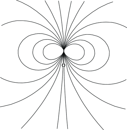
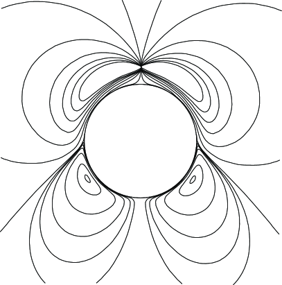
Figure 1: Field lines of the magnetic dipole placed (a) far away from the extreme Reissner-Nordström black hole, (b) close to the hole (from [8]).

3 The flux of stationary magnetic fields across rotating black holes

In order to investigate the structure of an asymptotically uniform test magnetic field on the background of a Kerr black hole we can start from the field $F_{\mu\nu}$ given explicitly in [18]. Without repeating here complicated formulas, let us recall that each $F_{\mu\nu}$ can be expressed as a sum of two terms, one being proportional to $B_{0}$, the magnitude of the component of the field asymptotically aligned with the hole’s rotation axis, the other, $B_{1}$, being the magnitude of the component perpendicular to the axis. Following Christodoulou and Ruffini [17] we define the magnetic (electric) lines of force as the lines tangent to the direction of the Lorentz force experienced by a test magnetic (electric) charge at rest with respect to the locally non-rotating frame. For the magnetic field lines this definition yields $dr/d\theta=-F_{\theta\phi}/F_{r\phi}\equiv B_{r}/B_{\theta}$ and $dr/d\phi=F_{\theta\phi}/F_{r\theta}\equiv B_{r}/B_{\phi}$.

(a)                                                     (b)
   
(c)                                                     (d)

Figure 2: Field lines of the test magnetic field homogeneous at infinity and aligned with hole’s rotation axis. Four cases with (a) $a=0.5M$ (b) $a=0.9M$ (c) $a=0.998M$ and (d) $a=M$ are shown. Notice that only a weak flux expulsion takes place for the cases (a) and (b). (Individual field lines start at $z=r\cos\theta=4$; they are separated by $0.1M$.)

In the case of the aligned field we can easily verify (by using $F_{\mu\nu}$ from [18]) that the field lines lie on the surfaces of constant flux,

$$\phi=\pi B_{0}[\Delta+2Mr\Sigma^{-1}\left(r^{2}-a^{2}\right)]\sin^{2}\theta={\rm constant},$$ (4)

where

$$\Delta=r^{2}-2Mr+a^{2},\,\,\,\Sigma=r^{2}+a^{2}\cos^{2}\theta;$$ (5)

$r,\theta,\phi$ are Boyer-Lindquist coordinates. The field lines constructed numerically are shown in Figure 2. The figures clearly illustrate how the magnetic field is expelled from the horizon when the angular momentum of the hole increases. Analogously to the Reissner-Nordström case, no field line of the asymptotically uniform magnetic field enters the horizon of an extreme Kerr black hole.

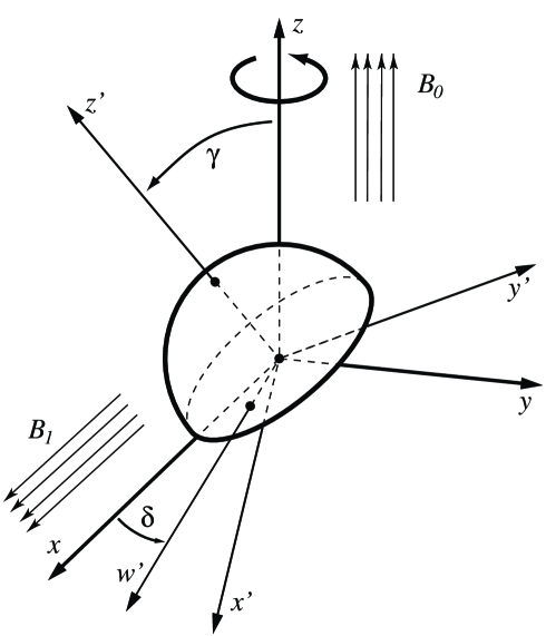
Figure 3: A generally located hemisphere across which the magnetic flux of an asympotically uniform magnetic field is calculated. The location of the hemisphere is specified by the angle $\gamma$ between the $z^{\prime}$-axis around which the hemisphere is rotationally symmetric and the $z$-axis around which the black hole rotates, and by the angle $\delta$ between the projection of the $z^{\prime}$-axis onto the equatorial plane and the $x$-axis along which is aligned the component of field, $B_{1}$, which is perpendicular to the rotation axis of the hole. $B_{0}$ is the component along this axis. (From [18].)

In the case of general stationary axisymmetric (i.e. “aligned”) electromagnetic fields, one arives, using solutions given in [19] (in the Newman-Penrose formalism), at a similar result: the flux of an arbitrary, axially symmetric stationary magnetic field across any part of the horizon of an extreme Kerr black hole vanishes.

The structure of an asymptotically non-aligned field is much more complicated. In this case $B_{\phi}\not=0$ and the field lines are dragged around the black hole. The lines, originally parallel to each other, are twisted, some of them threading the horizon even in an extreme case. The results of the numerical construction of the magnetic lines asymptotically perpendicular to the rotation axis of the Kerr black hole with $a/M=0.998$, as they look in the equatorial plane when viewed from above, are given in [20]. The field lines in Boyer-Lindquist coordinates are wound up around the horizon; in the Kerr ingoing coordinates the field lines do not wind up.

The structure of the magnetic field near a black hole can be characterized by the magnetic flux across (half of) the horizon. A general position of the hemisphere can be specified on the basis of an Euclidean picture. The magnetic flux across the hemisphere can be defined invariantly as an integral over the surface of the horizon [18]

$$\Phi=\int^{2\pi}_{0}\!\!\!\!\!d\phi\int^{\Theta(\phi;\gamma,\delta)}_{0}\!\!\!\!\!\!\!\!\!\!\!\!d\theta~{}{F_{\theta\phi}}_{|r=r_{+}},$$ (6)

where $\Theta(\phi;\gamma,\delta)\equiv\frac{\pi}{2}+\arctan[\tan\gamma\cos(\phi-\delta)]$ - see Figure 3.

Substituting for $F_{\theta\phi}$ and performing the integral we find rather complicated expression which, however, can be understood intuitively in special cases: (i) If $\gamma=0$ the magnetic flux reduces to $\Phi=B_{0}\pi r_{+}^{2}(1-a^{4}/r_{+}^{4})$; with $\gamma=0$ the total flux of the $B_{1}$ component of course vanishes. As the hole becomes extreme we find $\Phi\rightarrow 0$ – see Figure 2 (c-d). (ii) If $\gamma=\pi/2$ the flux is $\Phi=B_{1}\pi[r_{+}^{2}\cos\delta-(r_{+}+M)a\sin\delta]$. If the hole is not rotating one gets $\Phi=B_{1}\pi r_{+}^{2}\cos\delta=\Phi_{\rm classical}$. We get zero flux for $\delta=\pi/2$ and maximal one for $\delta=0$. When the hole rotates the field lines are dragged along and the flux vanishes across the hemisphere rotated by an angle $(\pi/2)-\delta_{0}$ where $\delta_{0}\sim 27^{o}$ for $a=M>0$. For a given $a$ there exists $\delta_{\rm max}$ for which the flux is maximal. With $a=M$ we find $\delta_{\rm max}\sim-63^{o}$, $\Phi\sim 2.25B_{1}\pi r_{+}^{2}=2.25\Phi_{\rm classical}$. Hence, we see that although the flux of the aligned component $B_{0}$ decreases to zero with $a\rightarrow M$, the flux of the perpendicular component is enhanced.

4 Magnetic flux across the stretched horizon of an almost extreme Kerr black hole

In this section we shall outline some results of [21] and of the discussions one of us (J.B.) had with Richard Price in 1996. The discussions were concerned with the validity of the membrane paradigm [1] for “alex” black holes, as we call “almost extreme” black holes. It is well-known that a proper distance from any point outside an extreme black hole to the outer horizon is infinite. This fact implied the statement in [1], p. 120, that “because the horizon is infinitely far down in the [embedding] diagram, the finite magnetic flux has an infinite spatial distance in which to wrap itself around the embedding cylinder, and, consequently, near the horizon the magnetic field falls off to zero.”

Notice, first, that in fact in a freely falling frame the component $B_{(\theta)}$ and $B_{(\varphi)}=-B_{(\theta)}\cos\theta$ do not vanish at the horizon of an extreme Kerr black hole, only the radial component $B_{(r)}=0$. (In case of an extreme Reissner-Nordström black hole all components of magnetic field do vanish even in a freely falling frame at the horizon.) Now in the spirit of the “membrane paradigm” consider a flux across a stretched horizon characterized (in the Boyer-Lindquist coordinates) by the redshift factor for locally non-rotating frames (“lapse function”),

$$\alpha=\left[(r^{2}+a^{2}\cos^{2}\theta)\Delta\right]^{\frac{1}{2}}\left[(r^{2}+a^{2})^{2}-a^{2}\Delta\sin^{2}\theta\right]^{-\frac{1}{2}},$$ (7)

which at a stretched horizon is small, $\alpha_{Hs}={\rm constant}\ll 1$, but nonvanishing - in contrast to the true horizon for which $\alpha_{Ht}=0$. Introduce a parameter $\epsilon=1-a/M$ so that $\epsilon$ is small for alex black holes and vanishes for the extreme holes. We know that the magnetic flux of axisymmetric fields vanishes at the true horizon in the limit $\epsilon\to 0$:

$$\lim_{\epsilon\to 0}\phi_{|\alpha_{Ht}=0}=0.$$ (8)

A question arises whether if we “exchange” the limits, i.e., calculate first the flux across the stretched horizon of an alex black hole and then go to the extreme case we could obtain a nonvanishing quantity: will then

$$\lim_{\alpha_{Hs}\rightarrow 0}\left(~{}\lim_{\epsilon\rightarrow 0}{\phi_{|\alpha_{H_{s}\not=0}}}~{}\right)\not=0~{}?$$ (9)

Restricting ourselves to asymptotically uniform fields we can easily calculate the flux across the stretched horizon (using the expressions for electromagnetic field given in [18]) and find that

$$\Phi\approx 8\pi B_{0}M^{2}\alpha_{H}~{}~{}{\rm for}~{}~{}\epsilon\ll\alpha^{2}_{H}~{},~{}~{}~{}~{}\Phi\approx 4\pi B_{0}M^{2}(2\epsilon)^{\frac{1}{2}}~{}~{}{\rm for}~{}~{}\epsilon\gg\alpha^{2}_{H}\,.$$ (10)

Therefore, $\Phi$ across the stretched horizon is nonvanishing even in the extreme case $\epsilon=0$ but it depends on where $H_{s}$ is located; however, $\Phi\rightarrow 0$ as $\alpha_{Hs}\rightarrow 0$, so that the limit (9) vanishes. For any $\epsilon>0$ there exists $\delta>0$ such that $\alpha_{H}<\delta$ and $\Phi<\epsilon$. This conclusion seems to suggest that power in the Blandford-Znajek model arises from regions with “relatively large” $\alpha_{H}$ in near-extreme case.

5 Black holes in magnetic fields: exact models

We now turn to the exact stationary solutions of the Einstein-Maxwell equations representing rotating, charged black holes immersed in an axisymmetric magnetic field. In the weak-field limit – when $\beta\equiv B_{0}M\ll 1$, the constant $B_{0}$ in the weak-field limit characterizes the magnetic field strength, $M$ the hole’s mass – there exists a region $2M\ll r\ll{B_{0}}^{-1}$ where the spacetimes are approximately flat and the magnetic field is approximately uniform. At $r\gg B_{0}^{-1}$ the metrics approach Melvin’s magnetic universe.

The simplest example is the magnetized Schwarzschild black hole:

$$ds^{2}=\Lambda^{2}\{(1-2M/r)^{-1}dr^{2}+r^{2}d\theta^{2}-(1-2M/r)dt^{2}\}+\Lambda^{-2}r^{2}\sin^{2}\theta\,\,d\phi^{2},$$ (11)

where $\Lambda=1+\frac{1}{4}B^{2}_{0}r^{2}\sin^{2}\theta$, the electromagnetic field being given by $F_{\theta\phi}\equiv B_{r}=B_{0}\Lambda^{-2}r^{2}\sin\theta\cos\theta$, $F_{r\phi}\equiv-B_{\theta}=B_{0}\Lambda^{-2}r\sin^{2}\theta$. The magnetic flux across a general hemisphere on the horizon (with $\delta=0$ due to axisymmetry, cf. Figure 3) reads as follows:

$$\Phi=4\pi\beta M\left[1+\beta^{2}\right]^{-\frac{1}{2}}\left[1+\beta^{2}+\tan^{2}\gamma\right]^{-\frac{1}{2}}.$$ (12)

For the flux across the “upper half” of the horizon $(\gamma=0)$, we obtain the result given in [18]. (See Eq. (41) therein where incorrect $M$ should be replaced by $r_{+}=2M$ in the denominator.)

If $\beta\ll 1$ the flux is equal to $4\pi\beta M(1+\tan^{2}\gamma)^{-\frac{1}{2}}$ in accordance with the weak-field approximation. By increasing $\beta$ (with $M$ and $\gamma$ fixed) $\Phi$ first increases, as we expect on classical grounds. However, a further increase of $\beta$ leads to the decrease of the flux. Indeed, there exists a value of the magnetic field parameter $\beta$ for which the flux acquires its maximum value, $\beta=(1+\tan^{2}\gamma)^{\frac{1}{4}}$. The global maximum, occurring with $\gamma=0$, is

$$\Phi=\Phi_{max}\equiv 2\pi M\doteq 3.22\times 10^{39}(M/10^{9}M_{\odot})\left[{\rm Gauss\;cm^{2}}\right].$$ (13)

The existence of the limiting value of the magnetic flux across the horizon is caused by the gravitational effect of the magnetic field which concentrates itself near the axis of symmetry when $\beta\gg 1$.

In [6], a rather exotic but interesting model was presented recently in which a supermassive black hole is surrounded by a superstrong magnetic field of the strength corresponding to just the half of the maximal flux (13). In this model an electric induction field can accelerate charged particles up to an energy $10^{18}$ GeV.

There exists a fairly extensive literature on exact solutions representing rotating charged black holes in an external magnetic field (a magnetic Melvin-type universe). They can be used to study the Meissner effect within the exact framework. One can make sure that the magnetic fluxes vanish across the horizons of extreme black holes, i.e. those with zero surface gravity. We refer to [22] and to very recent paper [23] for the review and relevant references.

6 Meissner effect for superconducting branes and extremal black holes in string theory

In 1998 a comprehensive paper by Chamblin, Emparan and Gibbons [24] reviewed and developed evidence for the Meissner effect for extremal black hole solutions in string theory and Kaluza-Klein theory. Here we shall mention some of their ideas and results, sticking closely to their discussion. They first give a brief phenomenological description of the Meissner effect in superconductors. Using London equation

$$\vec{j}=-\,{\rm constant}~{}\vec{A}~{},$$ (14)

($\vec{j}$ - current, $~{}\vec{A}$ - vector potential), and Maxwell’s equations, one arrives at the equation

$$\nabla^{2}\vec{A}=\lambda^{2}\vec{A},$$ (15)

$\lambda={\rm constant}$, given by constants characterizing the material. The solution in one dimension, $A\sim\exp(-\lambda x)$, indicates that $\vec{A}$ (and thus the magnetic field as well) decreases exponentially as one goes from the surface into the superconductive material. This is the classical Meissner effect. We see that the expulsion of a magnetic field from extreme (standard) black holes is analogous – but there is a difference: no magnetic flux at all penetrates into a hole. The relativistic generalization of the London equation reads

$$J_{\mu}=-\lambda^{-2}A_{\mu}+\partial_{\mu}\Lambda,$$ (16)

or

$$-\lambda^{-2}F_{\mu\nu}=\partial_{\mu}J_{\nu}-\partial_{\nu}J_{\mu},$$ (17)

where $J_{\mu}$ is $4$-current and $A_{\mu}$ 4-potential. In [24] equation (17) is adopted as the criterion for superconductivity. The authors first review the work of Nielsen and others showing that this equation is satisfied in the Kaluza-Klein theory on the world volume of extended objects carrying Kaluza-Klein currents. Then they consider self-gravitating extended superconducting objects and demonstrate how the flux of a gauge field is expelled from the intersection of two sets of 6-dimensional self-gravitating branes of 11-dimensional supergravity.

Several examples are then constructed in [24] demonstrating that the expulsion of gauge fields occurs always at the extreme horizon. Consider a string in $d=5$ which is wrapped along the string direction so that a dilatonic black hole solution in $d=4$ arises. The starting metric in $d=5$ reads

$$ds^{2}=H^{-\frac{1}{3}}\left(-fdt^{2}+dz^{2}\right)+H^{\frac{2}{3}}\left[f^{-1}dr^{2}+r^{2}\left(d\theta^{2}+\sin^{2}\theta d\varphi^{2}\right)\right],$$ (18)

where

$$H=1+q/r,\,\,\,f=1-r_{0}/r,$$ (19)

$q,r_{0}$ are constants, an event horizon being at $r=r_{0}$;  $r_{0}=0$ is the extreme case. If this geometry is compactified along the string direction $z$ in such a way that the compactification direction is twisted – the compactification is made along the orbits of the vector $(\partial/\partial z)+B(\partial/\partial\varphi)$, where constant $B$ will describe the asymptotic value of the magnetic field along the axis – one obtains a black hole and the Kaluza-Klein magnetic field. The field is described by the potential whose $\varphi$ - component is given by

$${\cal{A}}=Bg_{\varphi\varphi}/(g_{zz}+B^{2}g_{\varphi\varphi})=BHr^{2}\sin^{2}\theta/(1+B^{2}Hr^{2}\sin^{2}\theta).$$ (20)

In general one finds a non-vanishing flux across the horizon at $r=r_{0}$. In the limit of an extreme hole, however, at the horizon $r=0$ the potential ${\cal{A}}$ vanishes and no magnetic flux thus penetrates the horizon.

As another example of the Meissner effect Chamblin, Emparan and Gibbons consider the field expulsion from extreme rotating black holes. First they recall the expulsion of the asymptotic uniform magnetic test field in the extreme Kerr black hole background discussed in Section 3. Then they construct an exact solution (by taking the product of the standard Kerr solution with $x^{5}$-direction and applying a twisted reduction procedure, similar to that considered above but involving also a twist in the time coordinate) representing a Kerr black hole in the exact Kaluza-Klein gauge field. Again, this exact field exhibits the Meissner effect in the extreme case.

At the end of the subsection (see [24], V. A.) the authors write that they considered the solutions in which the magnetic field is aligned with the rotation axis of the black hole but that according to our work [8] the Meissner expulsion can also be seen for fields where no alignment is assumed. This is not correct: as mentioned in the previous Section 3, and demonstrated in detail in [18], the asymptotically non-aligned fields do penetrate the extreme Kerr horizons. Only general axisymmetric, stationary fields on the Kerr background exhibit the Meissner effect in the extreme limit. On the other hand, it is well known that configurations with stationary external fields which are not axisymmetric, are not stable – due to the torque exerted on the horizon by an external non-axisymmetric field (see e.g. [1]) – and evolve towards axisymmetric configurations.

In case of the standard superconductivity, when the Meissner effect arises, the field inside a superconductor becomes a pure gauge. This is not the case with extreme black holes. In [8] in Figure 1(d) the field lines are constructed inside the extreme Reissner-Nordström horizon. Clearly, one cannot claim that the interior of extreme black holes is in a superconducting state.

The question of the flux expulsion from the horizons of extreme black holes in more general frameworks is not yet understood properly. The authors of [24] “believe this to be a generic phenomenon for black holes in theories with more complicated field content, although a precise specification of the dynamical situations where this effect is present seems to be out of reach.” That for abelian Higgs vortices the phenomenon of flux expulsion from extreme black holes does not occur in all cases has been argued analytically and investigated numerically recently [25]. In particular, it appears that thin cosmic strings (modelled by the vortices) can pierce the extreme horizons whereas a thicker string will be expelled.

Acknowledgments. The authors are grateful to the organizers of the 3rd ICRA Workshop for their hospitality. Support from the grant No. GAČR 202/99/0261 of the Czech Republic and the grant GAUK 141/2000 of the Charles University is also gratefully acknowledged.

References

- [1] \BYThorne, K. S., Price, R. H. \atqueMacDonald, D. A. \TITLEBlack Holes: The Membrane Paradigm, (Yale University Press, New Haven) (1986).
- [2] \BYBurko, L., Ori, A. \TITLEIntroduction to the internal structure of black holes, in \TITLEInternal Structure of Black Holes and Spacetime Singularities, eds. \NAMEL. Burko \atqueA. Ori, (Inst. Phys. Publ., Bristol and The Israel Physical Society, Jerusalem) 1997.
- [3] \BYMirabel, I. F., Rodríguez, L. F. Microquasars in our Galaxy, \INNature 392 1998 673.
- [4] \BYPunsly, B., Coroniti, F. V. Relativistic winds from pulsar and black hole magnetospheres, \INAstrophys. J.3501990518. See also \BYPunsly, B. High-energy gamma-ray emission from galactic Kerr-Newman black holes. The central engine, \INAstrophys. J.4981998640, and references therein.
- [5] \BYLee, H. K., Wijers, R. A. M. \atqueBrown, G. E. The Blandford-Znajek process as a central engine for a gamma-ray burst, \INPhys. Reports325200083.
- [6] \BYKardashev, N. S. Cosmic supercollider \INMon. Not. R. Astron. Soc.276 1995515.
- [7] \BYFrolov, V., Novikov, I. \TITLEPhysics of Black Holes, (Kluwer, Dordrecht) 1998.
- [8] \BYBičák, J., Dvořák, L. Stationary electromagnetic fields around black holes III. General solutions and the fields of current loops near the Reissner-Nordström black hole, \INPhys. Rev. D2219802933.
- [9] \BYChandrasekhar, S. \TITLEThe Mathematical Theory of Black Holes, (Clarendon Press, Oxford) 1984.
- [10] \BYBičák, J. On the theories of the interacting perturbations of the Reissner-Nordström black hole, \INCzechosl. J. Phys. B291979945.
- [11] \BYBičák, J. \TITLEPerturbations of the Reissner-Nordtröm black hole, in \TITLEProceedings of the 2nd M. Grossmann Meeting on General Relativity, ed. \NAMER. Ruffini, (North Holland) 1982, p. 277.
- [12] \BYBičák, J. The motion of a charged black hole in an electromagnetic field, \INProc. Roy. Soc. Lond. A3711980429.
- [13] \BYBurko, L. M. Dipole perturbations of the Reissner-Nordström solution: The Polar Case, \INPhys. Rev. D 52 1995 4518.
- [14] \BYBurko, L. M. Dipole perturbations of the Reissner-Nordström solution: The axial case \INPhys. Rev. D 59 1999 084003.
- [15] \BYBičák, J. Stationary interacting fields around an extreme Reissner-Nordström black hole, \INPhys. Lett.64A1977279.
- [16] \BYKing, M., Pfister, H. On Electromagnetic Thirring Problems, to be submitted to Phys. Rev. D.
- [17] \BYChristodoulou, D., Ruffini, R. \TITLEOn the Electrodynamics of Collapsed Objects, in \TITLEBlack Holes, eds. \NAMEC.DeWitt \atqueB. deWitt (Gordon and Breach, London) 1973.
- [18] \BYBičák, J., Janiš, V. Magnetic fluxes across black holes, \INMon. Not. Roy. Astron. Soc. 212 1985899.
- [19] \BYBičák, J., Dvořák, L. Stationary electromagnetic fields around black holes II. General solutions and the fields of some special sources near a Kerr black hole, \INGen. Rel. Grav.71976959.
- [20] \BYKaras, V. Assymptotically uniform magnetic field near a Kerr black hole \INPhys. Rev. D4019892121.
- [21] \BYPrice, R. H. Some Developments in Black Hole Astrophysics, \INAnn. N.Y. Acad. Sci.6311991235.
- [22] \BYBičák, J., Karas, V. \TITLEThe influence of black holes on uniform magnetic fields, in \TITLEProc. of 5th M. Grossmann Meeting in General Relativity, eds. \NAMED. Blair et al (World Scientific, Singapore) 1989, p. 1199.
- [23] \BYKaras, V., Budínová, Z. Magnetic Fluxes Across Black Holes in a Strong Magnetic Field Regime, \INPhysica Scripta612000253.
- [24] \BYChamblin, A., Emparan, R. \atqueGibbons, G. W. Superconducting p-branes and extremal black holes, \INPhys. Rev. D581998084009.
- [25] \BYBonjour, F., Emparan, R. \atqueGregory, R. Vortices and extreme black holes: the question of flux expulsion, \INPhys. Rev. D591999084022