[

Resonance enhancement of particle production during reheating

Abstract

We found a consistent equation of reheating after inflation which shows that for small quantum fluctuations the frequencies of resonance are slighted different from the standard ones. Quantum interference is taken into account and we found that at large fluctuations the process mimics very well the usual parametric resonance but proceed in a different dynamical way. The analysis is made in a toy quantum mechanical model and we discuss further its extension to quantum field theory.

]

Inflation has become one of the most successful ideas of high energy cosmology today [1]. Actually most of the current work on experimental cosmology are based on ideas, or designed to test inflationary models [2]. No matter which inflationary model we assume, at the end of this period, it must reheat the universe. This period, called reheating, is very important because basically all elementary particles populating the universe were created. Much of the current interest in reheating follows after the discovery of an exponential amplification in the number of the particles produced during preheating. Source of this exponential growth is the presence of  the parametric and stochastic resonance [3, 4, 5, 6, 7] in the solutions of the equations of motion. Recent investigations address the problem of parametric amplification of super-horizon perturbations [8] during preheating and their consequences in the CMB spectrum [9].

Because the study of models of interacting fields evolving along the expansion of the universe is a highly non-trivial issue, analytical progress in this direction has been difficult to obtain. However, as we describe later, most of the main features of the observed phenomena can be obtained by studying a toy quantum mechanical model of two bi-quadratically coupled oscillators. Furthermore the recent interest in amplification of fluctuations can be described in this context.

In this letter, we describe in a simple way how parametric and stochastic resonance arise from the dynamics of a system of two coupled oscillators and we also identify the main problems that occur with the standard approaches, such as the energy conservation problem. We derive further in a consistent way, a semiclassical equation of motion for the scalar condensate field $R(t)$ (see Eq.(11) below). From the analysis of this equation, it is shown that the preheating phase proceeds in a different dynamical way, consistent with the Heisenberg’s principle. This fact also leads to appropriate initial conditions - an initially non-zero value for the fluctuations - to allow an efficient energy transfer between the oscillators. The equations obtained (Eq.(10) and Eq.(11)) can be considered as a classical system, allowing us to perform a complete numerical study [10]. A first numerical study shows a novel saturation effect in the small $R$-region of the equation for the fluctuation. This effect holds at the beginning of the energy transfer between the oscillators. We extend our results to quantum field theory, and take into account the expansion of the universe. This is straightforward, and the results obtained in our previous analysis can be extended with slight modifications.

The model we consider is a classical oscillator $X$ interacting with a purely quantum mechanical oscillator $\hat{Y}$ described by the Lagrangian

$$L=\frac{1}{2}\dot{X}^{2}+\frac{1}{2}\dot{\hat{Y}}^{2}-\frac{1}{2}\omega^{2}X^{2}-\frac{1}{2}\Omega^{2}\hat{Y}^{2}-\frac{1}{2}g^{2}X^{2}\hat{Y}^{2},$$ (1)

where $X(t)$ corresponds to the classical inflaton field $\phi(t)$ and $\hat{Y}(t)$ the created scalar field $\hat{\chi}(x)$ of inflationary cosmology respectively. For reasons of simplicity we will first neglect the expansion of the universe, and discuss at the end the effects and possible modifications of including such a friction term. The equations of motion are then corresponding to two coupled harmonic oscillators with time-dependent frequencies

$$\ddot{X}+(\omega^{2}+g^{2}\hat{Y}^{2})X=0,$$ (2)

$$\ddot{\hat{Y}}+(\Omega^{2}+g^{2}X^{2})\hat{Y}=0.$$ (3)

Let us now introduce time-independent creation and annihilation Heisenberg operators $a^{\dagger}$ and $a$ respectively using the Ansatz

$$\hat{Y}=f(t)a+f^{\ast}(t)a^{\dagger},$$ (4)

where, due to the standard commutator $\left[a,a^{\dagger}\right]=1$ for creation-annihilation operators, $f(t)$ satisfies the Wronskian condition

$$\dot{f}^{\ast}(t)f(t)-f^{\ast}(t)\dot{f}(t)=-i.$$ (5)

Inserting the Ansatz of Eq. (4) into Eq. (3), we find that $f(t)$ satisfies the equation of motion

$$\ddot{f}(t)+(\Omega^{2}+g^{2}X^{2}(t))f(t)=0,$$ (6)

where the normalization is fixed by the condition (5). If we consider $\hat{Y}$ in the frame of quantum field theory, Eq. (6) would be the equation for the zero-momentum term of its Fourier expansion. Motivated by the plane wave expansion of a quantized-field operator we use the following Ansatz for the function-coefficient $f(t)$

$$f(t)=\frac{1}{\sqrt{2W(t)}}\exp\left(-i\int^{t}W(t^{\prime})dt^{\prime}\right),$$ (7)

which satisfies automatically Eq. (5). Inserting this Ansatz into Eq. (6), we obtain the nonlinear differential equation for $W(t)$

$$\frac{1}{2}\frac{\ddot{W}}{W}-\frac{3}{4}\left(\frac{\dot{W}}{W}\right)^{2}+W^{2}=m^{2}(t),$$ (8)

where $m^{2}(t)=\Omega^{2}+g^{2}X^{2}(t)$. Eq. (8) describes a non-linear dissipative differential equation for $W(t)$. Instead of solving this rather cumbersome equation numerically, we will consider the Hamiltonian associated to the Lagrangian of Eq. (1) and construct a classical effective Hamiltonian by projecting onto the subspace of the number operator $\hat{n}=a^{\dagger}a$, generated by $\{\left|4\right\rangle,\left|3\right\rangle,\left|2\right\rangle,\left|1\right\rangle,\left|0\right\rangle\}$, which we will call $S_{5}$. The vacuum is as usual defined by the condition $a\left|0\right\rangle=0$. The choice of the non-trivial subspace $S_{5}$ is two fold. First, it attempts a fully quantum-mechanical treatment of this problem, allowing the possibility of quantum interference and other quantum effects in the effective classical theory, and secondly it allows an exact analitical solution of the quantum sector of the model. We first define the classical variable $R^{2}(t)=\left\langle 0\left|\hat{Y}^{2}\right|0\right\rangle$. The operator $\hat{Y^{2}}$ reads

$\displaystyle\left[\hat{Y}^{2}\right]_{nm}=\left[\begin{array}[]{ccccc}\left|f\right|^{2}&0&\sqrt{2}f^{2}&0&0\\ 0&3\left|f\right|^{2}&0&\sqrt{6}f^{2}&0\\ \sqrt{2}f^{\ast 2}&0&5\left|f\right|^{2}&0&2\sqrt{3}f^{2}\\ 0&\sqrt{6}f^{\ast 2}&0&7\left|f\right|^{2}&0\\ 0&0&2\sqrt{3}f^{\ast 2}&0&9\left|f\right|^{2}\end{array}\right].$

and can be diagonalized in $S_{5}$ explicitly $\left[\hat{Y}^{2}\right]_{nm}V_{i}=\lambda_{i}V_{i}$, where $V_{i}$ and $\lambda_{i}$ are the eigenvectors and eigenvalues respectively. Because of the similar structure of both operators, $\hat{Y}^{2}$ and $\hat{P}_{Y}^{2}=\dot{\hat{Y}}^{2}$, we can use the Ansatz of Eq. (4), and the effective Hamiltonian can be diagonalized exactly as

$$H_{ij}^{eff}=\frac{1}{2}[P_{X}^{2}+P_{R}^{2}+\frac{1}{4R^{2}}+\omega^{2}X^{2}+m^{2}(t)R^{2}]y_{i}\delta_{ij},$$ (9)

where $i,j=0,..4$. Up to irrelevant constants, this Hamiltonian describes the effective dynamics of two classical variables $X$ and $R$, which corresponds to the original classical and quantum oscillators. From Eq. (9) the equations of motion are

$$\ddot{X}+(\omega^{2}+g^{2}R^{2})X=0,$$ (10)

$$\ddot{R}+(\Omega^{2}+g^{2}X^{2}(t))R-\frac{1}{4R^{3}}=0.$$ (11)

The above equations actually correspond to two classical coupled particles-like degrees of freedom. Note that the centrifugal term keeps the fluctuation $R$ away from zero, consistent with Heisenberg’s principle and giving us appropriated natural initial conditions for numerical studies [10]. These equations are very simple and represent the starting point of our analysis.

A similar derivation of the classical Hamilton dynamics of a classical oscillator interacting with a quantum mechanical oscillator has been made in [11], in the context of semiquantum chaos. Nevertheless, the chosen classical-variable parametrization leads to cumbersome nonlinear dissipative differential equations.

We note here, that backreaction is taken into account in Eq. (10), through the dependence on the classical condensate variable $R$. We start the discussion of the classical dynamics by considering the perturbative regime of the equations of motion, at small coupling constant $g^{2}\ll 1$. For $g^{2}=0$, a solution of Eq. (10) is $X(t)=X_{0}\sin(\omega t)$. Inserting this expression into Eq. (6) we obtain a Mathieu equation

$$f^{\prime\prime}(z)+\left[A(q)-2q\cos 2z\right]f(z)=0,$$ (12)

where $z=\omega t$, $q=g^{2}X_{0}^{2}/4\omega^{2}$ and $A(q)=\Omega^{2}/\omega^{2}+2q$. This equation is well-known and has been used to discuss different mechanisms of particle production during the reheating period of the universe, such as parametric and stochastic resonance [3]-[6]. In fact, for $2q<A$ this equation leads to narrow parametric resonance [12] and for $2q>A$ leads to broad parametric resonance [4] (called stochastic resonance if expansion of the universe is considered). From the definitions above for $A$ and $q$, we observe that only the first region is allowed. The limit curve $A=2q$ in the space of parameters can be discussed by considering the limit case $\Omega^{2}=0$ of the equivalent equation

$$\ddot{f(t)}+(\Omega^{2}+g^{2}X_{0}^{2}\sin^{2}(\omega t))f(t)=0.$$ (13)

This equation leads also to a linear growth of the amplitude $f(t)$, close to the minimum of the potential for $X(t)$. This can be explained intuitively because this equation reads $\ddot{f}(t)=0$ at these points (see Fig. 1), and hence has solutions which raise linearly with time.

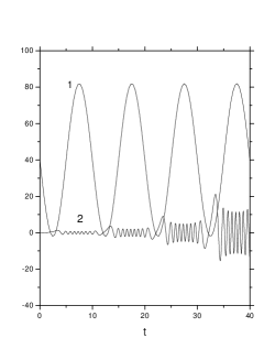
FIG. 1.: We show the oscillations of the source frequency (see Eq. (13)) which is responsible for parametric resonance (curve 1) and the response $f(t)$ (curve 2). Note that when the $X$ oscillations pass through zero, the maximun amplifications occur.

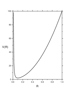
FIG. 2.: We plot the potential of Eq. (14) in a convenient scale. Note the the potential has a wall close to origen $R=0$.

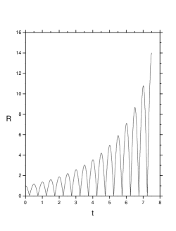
FIG. 3.: This plot shows the parametric amplification of $R$. In the context of a quantum field theory, this result is interpreted as a particle production process.

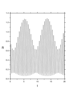
FIG. 4.: In the small amplitudes region, close to the resonance conditions, there is a novel saturation effect due to detuning coming from nonlinearities of the equation of motion. See explanation below Eq. (15).

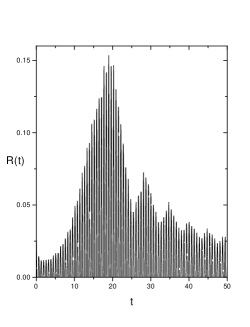
FIG. 5.: This plot shows how $R$ ceases to grow exponentially after certain time, when the expansion of the universe is considered. The resonance structure of the secondary maxima is given by the detuning effect due to the presence of the $a^{2}$-factor in the effective frequency term of Eq. (21).

However, it is natural to ask whether or not a non-exactly oscillatory form of $X$ will lead to an exponential growth of $f(t)$. Moreover, we know from this simple system that as soon as $f(t)$ start to growth, the functional form of $X$ will change, not only in amplitude but also in frequency. Also, attention must be down to solutions of Eq. (11) and not of Eq. (6), because in general its solutions does not satisfy the Wronskian condition Eq. (5). The best way to take into account the energy conservation, is by studying a numerical solution [10]. Even, the system (10,11) can be seen as a classical system allowing us to perform in a easier way such a study.

So, let us return to equations (10) and (11). The second equation can be interpreted as a particle moving in the presence of the potential

$$V(R)=\frac{1}{2}m^{2}(t)R^{2}+\frac{1}{8R^{2}}.$$ (14)

Figure 2 shows a plot of the potential for a convenient value of $m^{2}$. We see that $R=0$ acts as an infinite wall, which divides the coordinate space into two disconnected regions. Depending on which sign of the root we choose, the particle will remain in one of these two regions.

In order to analyze this potential, there are two scales to be considered. For large amplitudes $R\gg 1/\sqrt{2m}$, the potential looks essentially like a parabola with an infinite wall at $R=0$ (see Fig. 2). The solution of the equation without the non-linear term, which leads to the infinite wall, has resonances at $\Omega_{n}=2\omega/n$, as in the conventional parametric resonance (see [12]). One could naively expect to find resonances of the complete equation at twice this value because of the presence of the wall at $R=0$. But this is not true. The reason for this behavior is as follows. The solution of the problem without the wall-term is invariant under the shift $\omega t\rightarrow\omega t+\pi$. But this corresponds to the same solution of the system in the presence of the wall, when the phase is shifted by $\pi$ as $R$ approaches zero. Figure 3 shows the growth of the amplitude of oscillations for the main resonance band $\Omega=2\omega$. This curve has a similar shape and properties of the one corresponding to narrow parametric resonance, Fig. 2 in [5].

For small amplitudes $R\sim 1/\sqrt{2m}$, we can expand the potential around the time dependent minimum $R_{m}(t)=\pm 1/\sqrt{2m(t)}$

$$V(R)\simeq\frac{1}{2}m^{2}(t)+2(R-R_{m})^{2}m^{2}(t).$$ (15)

From (15), we see that for amplitude values close to the minimum, the potential develops a linear term, which leads to non-linear oscillations. Such oscillations hold in an almost energy conserved environment, because the amplitude of $R$ is small, so this effect is a genuine one and holds during the beginning of the transfer of energy. Fig. 4 shows the typical behavior of these oscillations. There are two regions separated by the size of the amplitude. When the amplitude is small and a resonance condition is fulfill, the linear term drives the system to larger values of the amplitude, which is characteristic of the broad parametric resonance (see Fig. 3 in [5]). Nevertheless, when the amplitude grows the non-linear term of the equation becomes important and breaks the resonance tuning and the growth of the amplitude saturates, while the amplitude starts to decrease. Most of the results obtained above can be still applied when we consider the expansion of the universe.

In quantum field theory the process follows similar lines. If we consider the inflaton field $\phi$ and the created field $\chi$ coupled minimally to gravity, the Lagrangian can be written as a sum ${\cal L}={\cal L}_{0}(\phi)+{\cal L}_{0}(\chi)+{\cal L}_{I}(\phi,\chi),$ where

$${\cal L}_{0}(\phi)=\sqrt{-g}[\frac{1}{2}(\partial\phi)^{2}-\frac{1}{2}m_{\phi}^{2}\phi^{2}],$$ (16)

where the interaction is ${\cal L}_{I}=-\frac{1}{2}g^{2}\phi^{2}\chi^{2}$. Let us consider $\phi(t)$ and $\chi(t)$ as homogeneous fields, but the former as a classical and the later as a quantum operator field. Assuming a flat FRW metric, the equations of motion obtained from the Lagrangian (16) are

$$\chi^{\prime\prime}+2{\cal H}\chi^{\prime}+a^{2}(M_{\chi}^{2}+g^{2}\phi^{2})\chi=0,$$ (17)

$$\phi^{\prime\prime}+2{\cal H}\phi^{\prime}+a^{2}(m_{\phi}^{2}+g^{2}\chi^{2})\phi=0,$$ (18)

where $a$ is the scale factor, a prime ^′ means a derivative respect to conformal time $\eta=\int dt/a(t)$, and ${\cal H}=a^{\prime}/a$. Defining the conformal fields as $X=a\phi$ and $\hat{Y}=a\chi$, we find the equations

$$X^{\prime\prime}+(a^{2}m_{\phi}^{2}+g^{2}\hat{Y}^{2}-\frac{a^{\prime\prime}}{a})X=0,$$ (19)

$$\hat{Y}^{\prime\prime}+(a^{2}M_{\chi}^{2}+g^{2}X^{2}-\frac{a^{\prime\prime}}{a})\hat{Y}=0.$$ (20)

If we neglect the coupling between $\chi$ with $\phi$ and during the oscillations of the inflaton, the universe expands as a one dominated by matter. Under such circunstances the last term inside the brackets can be dropped out. Moreover, we have checked numerically that the last term $a^{\prime\prime}/a$ can be neglected, even if the coupling is considered.

The semiclassical approximation leads to the equation

$$R^{\prime\prime}+(a^{2}M_{\chi}^{2}+g^{2}X^{2}-\frac{a^{\prime\prime}}{a})R-\frac{1}{4R^{3}}=0,$$ (21)

and similarly the corresponding for $X$ (Eq.(19)) but replacing $\hat{Y}^{2}$ by $R^{2}$. If we consider the corrections beyond the long-wavelenght limit of the field $\hat{Y}$, an infinite set of non-linear coupled differential equations for the modes $R_{k}$ prevents an analogous explicit description as the one given by Eq. (21). Nevertheless, this observation allows a perturbative treatment of this problem by a gradient expansion of the fields, but this is beyond the scope of our analysis. Because the fields are scaled by $a$, the expansion of the universe should damp the oscillations of the created field $R$ (or $\chi$) in Fig. 1 and Fig. 3. In Fig. 5 the combined effects of backreaction and the expansion of the universe in the evolution of the field $R$ is shown. As a consequence, $R$ ceases to grow exponentially, after certain time. The resonance structure of the secondary maxima can be explained by the detuning effect due to the presence of the scale factor in the effective frequency term of Eq. (21).

In this letter we have described a model to study reheating after inflation. We have showed that a simple model of two coupled oscillators can reproduce the main resonances effects, responsible for particle creation during preheating. In addition we have derived a semiclassical equation describing particle production consistent with Heisenberg’s uncertainty principle. From this equation we have also found that at small amplitude of the oscillations, i. e. when the energy transfer starts, there is no resonance amplification. This seems to indicate that there is an energy threshold to get efficient particle production.

REFERENCES

- [1] A. D. Linde, Particle Physics and Inflationary Cosmology, Harwood, NY (1990).
- [2] M. S. Turner and J. A. Tyson, Rev. Mod. Phys. 71, S145 (1999).
- [3] J. Traschen and R. Brandenberger, Phys. Rev. D 42, 2491 (1990).
- [4] L. A. Kofman, A. D. Linde, and A. A. Starobinsky, Phys. Rev. Lett. 73, 3195 (1994); 76, 1011 (1996).
- [5] L. A. Kofman, A. D. Linde, and A. A. Starobinsky, Phys. Rev. D 56, 3258 (1997).
- [6] Y. Shtanov, J. Traschen and R. Brandenberger, Phys. Rev. D 51, 5438 (1995).
- [7] D. Boyanovsky, H. J. de Vega, R. Holman, D. S. Lee, and A. Singh, Phys. Rev. D 51, 4419 (1995); D. Boyanovsky, M. D’Attanasio, H. J. de Vega, R. Holman, D. S. Lee, and A. Singh, ibid 52, 6805 (1995); D. Boyanovsky, H. J. de Vega, R. Holman, D. S. Lee, A. Singh, and J. F. Salgado, ibid 54, 7570 (1996).
- [8] B. Basset, D. Kaiser, and R. Maartens, Phys. Lett. B455, 84 (1999); B. Bassett, F. Tamburini, D. Kaiser, and R. Maartens, Nucl. Phys. B561, 188 (1999); B. Bassett, C. Gordon, R. Maartens, and D. Kaiser, Phys. Rev. D 61, 061302 (2000); F. Finelli and R. Brandenberger, hep-ph/0003172.
- [9] B. A. Bassett and F. Viniegra, Phys. Rev. D 62, 043507 (2000); J. P. Zibin, R. Brandenberger, and Douglas Scott, hep-ph/0007219.
- [10] S. E. Joras and V. H. Cárdenas, in preparation.
- [11] F. Cooper, J. Dawson, D. Meredith, and H. Shepard, Phys. Rev. Lett. 72, 1337 (1994); F. Cooper, J. Dawson, S. Habib and R. D. Ryne, Phys. Rev. E 57, 1489 (1998).
- [12] L. D. Landau y E. M. Lifshitz, Mecánica, Reverté, Barcelona (1970).