Parametrization of singularities of the Demiański-Newman spacetimes

Abstract

We propose a new presentation of the Demiański-Newman (DN) solution of the axisymmetric Einstein equations. We introduce new dimensionless parameters $p$, $q$ and $s$, but keeping the Boyer-Lindquist coordinate transformation used for the Kerr metric in the Ernst method. The family of DN metrics is studied and it is shown that the main role of $s$ is to determine the singularities, which we obtain by calculating the Riemann tensor components and the invariants of curvature. So, $s$ reveals itself as the parameter of the singular rings on the inner ergosphere.

PACS numbers: 04.70.Bw, 04.20.Dw, 04.20.Jb

I Introduction

The Kerr metric can be easily obtained from the Ernst equation [1],

$$(\xi\xi^{\ast}-1)\nabla^{2}\xi=2\xi^{\ast}\nabla\xi\cdot\nabla\xi,$$ (1)

where $\nabla$ denotes the usual three dimensional spatial operator and $\xi$ is a complex potential being function of $\lambda$ and $\mu$ which are the prolate spheroidal coordinates. By considering, as solution of Eq. (1),

$$\xi=p_{K}\lambda+iq_{K}\mu,$$ (2)

where $p_{K}$ and $q_{K}$ are real constants satisfying

$$p_{K}^{2}+q_{K}^{2}=1,$$ (3)

we can obtain the Kerr solution.

The theorem of Robinson-Carter (see p. 292 of Ref. [2]) demonstrates the uniqueness of this vacuum stationary axisymmetric solution with an asymptotically flat behavior and smooth convex event horizon without naked singularity. This solution is characterized by only two independent parameters, being the mass $M$ and the angular momentum $J=aM$, where $a$ is angular momentum per unit mass. The Kerr solution has an event horizon (or outer horizon), a Cauchy horizon (or inner horizon), an outer ergosphere (or stationary limit surface), an inner ergosphere and a ring singularity.

In this paper we propose to generalize the solution (2) by considering

$$\xi=p\lambda+\beta\mu+i(\gamma\lambda+q\mu),$$ (4)

where $p,\beta,\gamma$ and $q$ are real constants. The expression (4) is also solution of the Ernst equation and corresponds to the Demiański-Newman (DN) solution [3] as we shall see in Section II. The DN solution obtained through a complex transformation from the Kerr solution, namely the introduction of a constant phase factor (see (7) hereafter), has three independent parameters. The interpretation of the third parameter, usually denoted $l$, compared to just two parameters in the Kerr solution, is still not clear. In its place we introduce another parameter, which we call $s$, which parametrizes the singularities in a particularly simple way, as we shall see in Section IV. We write the corresponding metric in Section III.

II Choice of the parameters

The expression (4) is a solution of the equation (1) if the following conditions are satisfied

$$p^{2}+\beta^{2}+\gamma^{2}+q^{2} = 1,$$ (5)

$$p\beta = -\gamma q.$$ (6)

Let us recall that the DN solution [3] is usually presented [4] as

$$\xi=e^{ia_{1}}(p_{DN}\lambda+iq_{DN}\mu),$$ (7)

with

$$p_{DN}^{2}+q_{DN}^{2}=1,$$ (8)

where $p_{DN},q_{DN}$ and $a_{1}$ are real constants. The comparison between Eq. (4) and Eq. (7) imposes

$$p = p_{DN}\cos a_{1},\;\;q=q_{DN}\cos a_{1},$$ (9)

$$\beta = -q_{DN}\sin a_{1},\;\;\gamma=p_{DN}\sin a_{1}.$$ (10)

Then Eqs. (5)–(6) are automatically satisfied, i.e., there is an identity between Eq. (4) and Eq. (7). In order to write the DN metric in Boyer-Lindquist (BL) coordinates the following relations are usually considered (see p. 387 of Ref. [4]),

$$\lambda = \frac{r-M}{k_{DN}},\;\;\mu=\cos\theta,$$ (11)

$$p_{DN} = \frac{k_{DN}}{\sqrt{M^{2}+l^{2}}},\;\;q_{DN}=\frac{a}{\sqrt{M^{2}+l^{2}}},$$ (12)

$$\cos a_{1} = \frac{M}{\sqrt{M^{2}+l^{2}}},\;\;\sin a_{1}=\frac{l}{\sqrt{M^{2}+l^{2}}},$$ (13)

with

$$k_{DN}^{2}=M^{2}+l^{2}-a^{2},$$ (14)

where $l$ is a third parameter with mass dimension and $r$ and $\theta$ are spherical coordinates. When $l=0$, the DN metric becomes the Kerr metric.

Here, we shall not proceed in this way and the relations (7)–(14) will not be used. Instead, we shall present the DN solution as follows.

In place of Eq. (7), we consider the following complex transformation carried out on the Kerr solution,

$$\xi=e^{ia_{1}}(p_{K}\lambda+iq_{K}\mu),$$ (15)

where the variables $\lambda$ and $\mu$ are the Kerr’s ones.

This interpretation of the DN solution, as the Kerr solution with a phase factor, seems simpler and more natural to us. Indeed Eq. (4) is, for us, a simple linear extension of the Kerr solution of the Ernst equation.

Then, by identification between Eq. (15) and Eq. (4) we obtain relations identical to Eqs. (9)–(10), where $p_{DN}$ and $q_{DN}$ are simply replaced by $p_{K}$ and $q_{K}$ :

$$p = p_{K}\cos a_{1},\;\;q=q_{K}\cos a_{1},$$ (16)

$$\beta = -q_{K}\sin a_{1},\;\;\gamma=p_{K}\sin a_{1}.$$ (17)

These two Kerr parameters

$$p_{K}=\frac{k}{M},\;\;q_{K}=\frac{a}{M},$$ (18)

with

$$k^{2}=M^{2}-a^{2},$$ (19)

are linked to the two physical parameters $M$ and $a$. Note that $(p_{K},q_{K})$ are different from $(p_{DN},q_{DN})$ given in Eqs. (12), which are linked to the three parameters $M$, $a$ and $l$, though each couple obeys the same relation (8) or (3).

To the third parameter $a_{1}$, present in the DN solution (15), we associate the dimensionless parameter $s$ defined by

$$s^{2}=\frac{1}{\cos^{2}a_{1}},\;\;(s\geqslant 1).$$ (20)

So, the relations (16)–(17) become

$$p = \frac{p_{K}}{s}=\frac{k}{Ms},\;\;q=\frac{q_{K}}{s}=\frac{a}{Ms},$$ (21)

$$\frac{\gamma}{p} = -\frac{\beta}{q}=\sqrt{s^{2}-1}.$$ (22)

Note that relation (22) also holds from Eqs. (9)–(10), i.e., in the usual interpretation of the DN solution. With Eq. (22), relation (5) becomes

$$s^{2}(p^{2}+q^{2})=1,$$ (23)

which is also in agreement with Eqs. (21).

Finally, instead of Eqs. (11) with relation (14), we introduce BL coordinates,

$$\lambda=\frac{r-M}{k},\;\;\mu=\cos\theta.$$ (24)

where $k$ is defined in relation (19), which is the BL transformation used for the Kerr solution. In particular, the coordinates are the Kerr’s ones, coherently with the solution (15), which is not the case in the usual DN solution for which $\lambda$ depends on $l$ (compare Eqs. (11) with Eqs. (24)).

III Metric coefficients

The stationary axisymmetric metric, being in the Papapetrou form [4, 5], reads

$$ds^{2}=f(dt-\omega d\phi)^{2}-\frac{k^{2}}{f}\left[e^{2\gamma}(\lambda^{2}-\mu^{2})\left(\frac{d\lambda^{2}}{\lambda^{2}-1}+\frac{d\mu^{2}}{1-\mu^{2}}\right)+(\lambda^{2}-1)(1-\mu^{2})d\phi^{2}\right],$$ (25)

where $f,\omega$ and $\gamma$ are functions of $\lambda$ and $\mu$ only. The real part $P$ and the imaginary part $Q$ of $\xi$, given by the solution (4), become using relations (22),

$$P=p\lambda-q\sqrt{s^{2}-1}\mu,\;\;Q=p\sqrt{s^{2}-1}\lambda+q\mu.$$ (26)

The Ernst method [1, 4] to determine the metric consists to make a homographic transformation

$$\zeta=\frac{\xi-1}{\xi+1},$$ (27)

where $\zeta$ is of the form

$$\zeta=f+i\,\Omega,$$ (28)

with $f$ being the metric coefficient of the line element (25) and $\Omega$ being the so called twist potential linked to the dragging of spacetime, $\omega$, through the differential relations

$$\omega_{\lambda}^{\prime}=\frac{k(\mu^{2}-1)}{f^{2}}\Omega_{\mu}^{\prime},\;\;\omega_{\mu}^{\prime}=\frac{k(\lambda^{2}-1)}{f^{2}}\Omega_{\lambda}^{\prime},$$ (29)

where indexes indicate to which variable the differentiation, indicated by primes, is to be taken. Once the partial differential equations (29) are integrated we obtain $\omega$. Applying this method we have

$$f = \frac{s^{2}[q^{2}(\mu^{2}-1)+p^{2}(\lambda^{2}-1)]}{s^{2}(p^{2}\lambda^{2}+q^{2}\mu^{2})+2[p\lambda-\sqrt{s^{2}-1}q\mu]+1},$$ (30)

$$\omega = \frac{2k}{s^{2}p}\left[\frac{q(1+p\lambda)(1-\mu^{2})+p^{2}\sqrt{s^{2}-1}(1-\lambda^{2})\mu}{q^{2}(\mu^{2}-1)+p^{2}(\lambda^{2}-1)}\right].$$ (31)

From the field equations [1, 4] we also find

$$e^{2\gamma}=\frac{s^{2}(p^{2}\lambda^{2}+q^{2}\mu^{2})-1}{p^{2}(\lambda^{2}-\mu^{2})}.$$ (32)

Substituting the expressions for $p,q$ and $\lambda$, corresponding to Eqs. (21) and Eq. (24), into Eqs. (30)–(32), we obtain

$$f = \frac{s(r^{2}-2Mr+a^{2}\mu^{2})}{s(r^{2}+a^{2}\mu^{2})+2(s-1)M^{2}-2M[(s-1)r+\sqrt{s^{2}-1}a\mu]},$$ (33)

$$\omega = \frac{2M}{s(r^{2}-2Mr+a^{2}\mu^{2})}\left\{a(1-\mu^{2})[r+(s-1)M]-(r^{2}-2Mr+a^{2})\sqrt{s^{2}-1}\mu\right\},$$ (34)

$$e^{2\gamma} = \frac{s^{2}(r^{2}-2Mr+a^{2}\mu^{2})}{(M-r)^{2}-(M^{2}-a^{2})\mu^{2}}.$$ (35)

IV Singularities of the DN spacetime

We can write Eq. (33) like

$$f=\frac{N}{D},$$ (36)

where

$$N(r,\mu) = s[r-r_{-}(\mu)][r-r_{+}(\mu)],$$ (37)

$$D(r,\mu) = sr^{2}-2(s-1)Mr+sa^{2}\mu^{2}-2\sqrt{s^{2}-1}Ma\mu+2(s-1)M^{2},$$ (38)

with

$$r_{-}(\mu)=M-\sqrt{M^{2}-a^{2}\mu^{2}},\;\;r_{+}(\mu)=M+\sqrt{M^{2}-a^{2}\mu^{2}}.$$ (39)

The equations $r=r_{-}(\mu)$ and $r=r_{+}(\mu)$, producing $N=0$, define respectively the inner and outer ergospheres (see p. 316 of Ref. [2]). The inner horizon or Cauchy horizon, and the outer horizon or event horizon are given, respectively, by $r_{-}=M-\sqrt{M^{2}-a^{2}}$ and $r_{+}=M+\sqrt{M^{2}-a^{2}}$ (see p. 278 of Ref. [2]). $D=0$ defines the singularities of spacetime (see Appendix). In order to have this second order polynomial equation in $r$ satisfied, we need

$$r=\frac{1}{s}\left\{(s-1)M\pm\sqrt{-s^{2}a^{2}(\mu-\mu_{s})^{2}}\right\},$$ (40)

with

$$\mu_{s}=\sqrt{s^{2}-1}\frac{M}{sa}.$$ (41)

Hence, to Eq. (40) produce real roots, one needs

$$\mu=\mu_{s},$$ (42)

which defines the equation of a cone. In this case $\mu$ is fixed, for a given $s$, and we can now write $D$ with relation (42) like

$$D(r)=s(r-r_{s})^{2},$$ (43)

where

$$r_{s}=\frac{(s-1)M}{s}.$$ (44)

Then, according to Eq. (43), the only possible singular points for a given $s$ are distributed on a sphere with radius

$$r=r_{s}.$$ (45)

But at the same time, the singular points have to satisfy condition (42), and the intersection of the two folds of the cone with the sphere (45) produce two rings. Hence the singularities for DN spacetime are spread along two symmetrical rings centered at the $z$ axis. Therefore we can consider only the upper fold $\theta\in\left[0,\pi/2\right]$, remembering that we have to complete the picture by symmetry. Now, if we eliminate the parameter $s$ between the two equations (42) and (45), we obtain

$$r=M-\sqrt{M^{2}-a^{2}\mu^{2}},$$ (46)

which we recognize as the equation of the inner ergosphere given just after Eqs. (39). Hence, each value of $s$ corresponds to a ring singularity, which is a circle, being the intersection of the inner ergosphere with the cone (42), see Figure 1. The two circular rings are centered on the $z$ axis at $\pm z_{s}$, where

$$z_{s}=r_{s}\mu_{s}=(s-1)\sqrt{s^{2}-1}\frac{M^{2}}{s^{2}a},$$ (47)

and the radius $R_{s}$ of the two rings is

$$R_{s}=r_{s}\sin\theta_{s}=r_{s}\sqrt{1-\mu_{s}^{2}}=\frac{(s-1)M}{s}\sqrt{1-\frac{(s^{2}-1)M^{2}}{s^{2}a^{2}}}.$$ (48)

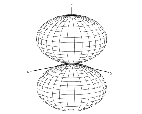
FIG. 1.: Inner ergosphere of DN spacetime for the following values, $a=4$ and $M=4.2$, of the parameters. The vertical axis of revolution is the $z$ axis. The orthogonal plane $xy$ contains the angle $\phi$, and $\theta$ is the angle between the $z$ axis and the position vector of a point in the space. The intersections of the planes $z=cte$ with the inner ergosphere are the ring singularities. For each value of $s$ there are two ring singularities, symmetrical with respect to the plane $xy$. For the Kerr metric $(s=1)$ the ring singularity is reduced to the origin $O$. For $s_{max}$, the two ring singularities are the poles on the $z$ axis.

We can say that $s$ parametrizes the singular rings, intersections of the inner ergosphere with a continuous foliation of planes orthogonal to the $z$ axis. For each value of $s$ there is a different spacetime, see Eqs. (33)–(35). In particular for $s=1$ we have the Kerr spacetime. However the inner ergosphere is the same, as well as the outer ergosphere and the two horizons, for all these metrics, i.e., for any $s$ (see Figure 2). Only the ring singularity changes with $s$, and each ring singularity belongs to the inner ergosphere.

FIG. 2.: Ergospheres (with solid lines) and horizons (with dashed lines) of DN spacetime for the following values, $a=4$ and $M=4.2$, of the parameters. We plot here the intersections of the plane $\phi=cte$ with the surfaces of revolution, obtained from the rotation of these curves around the $z$ axis. The radius of Cauchy horizon is here $r_{-}\simeq 2.92$, and the radius of the event horizon $r_{+}\simeq 5.48$.

By definition $0\leq\mu_{s}\leq 1$, hence from Eq. (41) we have

$$1\leq s\leq s_{max}=\frac{M}{\sqrt{M^{2}-a^{2}}},$$ (49)

and from Eq. (44) we have

$$0\leq r_{s}\leq r_{smax}=r_{-}=M-\sqrt{M^{2}-a^{2}}.$$ (50)

For $s=1$, which produces Kerr metric, we have from Eq. (44) $r_{s}=0$, or from Eq. (48) $R_{s}=0$. Hence the Kerr limit minimizes the radius of the ring singularity and reduces the two ring singularities to just one. The other metric that minimizes the radius (but produces two symmetrical ring singularities) happens when

$$s=s_{max}=\frac{M}{\sqrt{M^{2}-a^{2}}},$$ (51)

giving, from Eq. (41), $\mu_{s}=1$ and, from Eq. (48), $R_{s}=0$.

We can calculate the maximum radius $R_{smax}$ of the ring singularities given by the equation (48) for $R_{s}(s)$. Calculating $dR/ds$ we find the maximum which is for $s$ given by

$$s=\frac{-1+\sqrt{1+8(1-a^{2}/M^{2})}}{2(1-a^{2}/M^{2})}.$$ (52)

If $a\ll M$ we see from relation (49) that $1\leq s\leq s_{max}\approx 1+a^{2}/(2M^{2})$, hence up to first order $O(a/M)$ the spacetime reduces to Kerr spacetime. On the other hand, if $a=0$ and $s\neq 1$ we see that the spacetime reduces to Taub-NUT spacetime (see p. 387 of Ref. [4]) and $D(r)=0$ has no real roots for $r$, demonstrating that there are no singularities in this case.

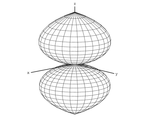
FIG. 3.: Inner ergosphere of a extreme DN black-hole for the following values, $a=M=4$, of the parameters. The intersections of the planes $z=cte$ with the inner ergosphere are the ring singularities. For each value of $s$ there are two ring singularities, symmetrical with respect to the plane $xy$.

FIG. 4.: Ergospheres (with solid lines) and horizons (with dashed lines) of a extreme DN black-hole for the following values, $a=M=4$, of the parameters. We plot here the intersections of the plane $\phi=cte$ with the surfaces of revolution, obtained from the rotation of these curves around the $z$ axis. Notice the continuity of the two ergospheres and of their slopes. The two horizons are the same, $r_{\pm}=M=4$.

Finally, for the so-called “extreme black hole” ($a=M$), equations (41), (47)–(49) give

$$\mu_{s}=\frac{\sqrt{s^{2}-1}}{s},\quad z_{s}=\frac{M(s-1)\sqrt{s^{2}-1}}{s^{2}},\quad R_{s}=\frac{M(s-1)}{s^{2}},\quad 1\leqslant s<\infty$$ (53)

respectively, see Figures 3 and 4. The metric which maximizes the radius of the ring singularity is obtained from condition (52) for $s=4$, and we obtain in this case

$$\mu_{s}=\frac{\sqrt{15}}{4}\ or\ \theta_{s}\simeq 14,48^{o},\quad r_{s}=\frac{3M}{4},\quad z_{s}=\frac{3\sqrt{15}M}{16},\quad R_{s}=\frac{3M}{16}.$$ (54)

V Conclusion

The usual presentation of the DN solution obtained from the Ernst equation introduces another BL transformation (11) instead of the Kerr’s one (24), and new parameters $(p_{DN},q_{DN})$ which are functions of $(M,a,l)$ and linked by the relation (8) of Kerr’s type.

In our interpretation of the DN solution, we keep the BL coordinate transformation of Kerr (24), but we introduce new parameters $(p,q)$ depending on $(M,a,s)$ and linked by relation (23) which is no longer of Kerr’s type.

Hence, the DN solution of the field equations for a given source $(a,M)$ constitutes a family of metrics which can be parametrized by a dimensionless parameter $s$ defined by equation (20). The Kerr solution $(s=1)$ belongs to this family.

We call generically “DN black hole” the set of ergospheres, horizons and singularities of this family.

Then, the only change that $s$ introduces on the DN black hole structure concerns the singularities. The ergospheres and horizons are the same for each metric of the DN family, i.e., whatever $s$, in particular for the Kerr metric $(s=1)$. $s$ parametrizes only each ring singularity, which always belongs to the inner ergosphere, including the limiting case of Kerr $(s=1)$.

So the Kerr metric appears as the one which minimizes the ring singularity.

Appendix

Here we present the components of $R_{\alpha\beta\gamma\delta}$ for the metric (25), transformed in spherical coordinates, with relations (33)–(35). The convention used for the Riemann tensor is $(R^{\alpha}{}_{\beta\gamma\delta}=-\Gamma^{\alpha}{}_{\beta\gamma,\delta}+...)$. Since the expressions become too long, we restrict to present only the denominators $d[R_{\alpha\beta\gamma\delta}]$ of its non null components. We use the definitions (37)–(38) and $\Delta=r^{2}-2Mr+a^{2}$ producing the following components :

$$d[R_{t\phi t\phi}] = 4sN^{2}D^{3},$$ (55)

$$d[R_{t\phi\theta r}] = 4\Delta ND^{2},$$ (56)

$$d[R_{t\theta t\theta}] = d[R_{t\theta tr}]=d[R_{trtr}]=4\Delta ND^{3},$$ (57)

$$d[R_{t\theta\phi\theta}] = d[R_{t\theta\phi r}]=d[R_{tr\phi\theta}]=d[R_{tr\phi r}]=4\Delta N^{2}D^{3},$$ (58)

$$d[R_{\phi\theta\phi\theta}] = d[R_{\phi\theta\phi r}]=d[R_{\phi r\phi r}]=4\Delta N^{3}D^{3},$$ (59)

$$d[R_{\theta r\theta r}] = 4\Delta D.$$ (60)

We see that the denominators of all components of the Riemann tensor become null only if $D=0$, i.e., when the relations (41)–(42), (44)–(45) are satisfied.

When $s=1$ we reobtain the components of the Riemann tensor for Kerr spacetime.

The calculation of the invariants of curvature ($R^{2}$, $R^{\alpha\beta}R_{\alpha\beta}$, $R^{\alpha\beta\gamma\delta}R_{\alpha\beta\gamma\delta}$, etc) confirms that the condition $D=0$ determines the singularities of DN spacetime.

REFERENCES

- [1] F. J. Ernst, Phys. Rev. 167, 166 (1968).
- [2] S. Chandrasekhar, The Mathematical Theory of Black Holes (Oxford University Press, Oxford 1983).
- [3] M. Demiański and E.T. Newman, Bull. Acad. Polon. Sci. Ser. Math. Astro. Phys. 14, 653 (1966).
- [4] M. Carmeli, Classical Fields: General Relativity and Gauge Theory (John Wiley and Sons, New York 1982).
- [5] A. Papapetrou, Ann. der Phys. 12, 309 (1953).