Electron-Positron Jets from a Critically Magnetized Black Hole

Abstract

The curved spacetime surrounding a rotating black hole dramatically alters the structure of nearby electromagnetic fields. The Wald field which is an asymptotically uniform magnetic field aligned with the angular momentum of the hole provides a convenient starting point to analyze the effects of radiative corrections on electrodynamics in curved spacetime. Since the curvature of the spacetime is small on the scale of the electron’s Compton wavelength, the tools of quantum field theory in flat spacetime are reliable and show that a rotating black hole immersed in a magnetic field approaching the quantum critical value of $B_{k}=m^{2}c^{3}/(e\hbar)\approx 4.4\times 10^{13}$ G $\approx 1.3\times 10^{-11}$ cm^-1 is unstable. Specifically, a maximally rotating three-solar-mass black hole immersed in a magnetic field of $2.3\times 10^{12}$ G would be a copious producer of electron-positron pairs with a luminosity of $3\times 10^{52}$ erg s^-1.

I Introduction

The recent discovery that gamma-ray bursts (GRBs) are associated with galaxies at cosmological distances has spurred the development of thoeretical models of the central engines of these objects which emit $\sim 10^{51-53}$ ergs (assuming isotropic emission) over the span of several to several hundred seconds. Some of the more popular models involve some sort of electromagnetic bomb: a quickly rotating, strongly magnetized neutron star (e.g. [1, 2]) or a rotating black hole threaded by a strong magnetic field (e.g. [3, 4, 5]). The first model extends the standard picture of radio pulsar spindown (e.g. [6]) to ultrastrong magnetic fields and high spin frequencies; the second model recasts the Blandford and Znajek [7] mechanism for the central engine of quasars in the realm of a stellar black hole accreting the debris of a tidally disrupted neutron star.

An examination of the instability of the magnetized vacuum surrounding a rotating black hole provides an excellent starting point to understanding these processes. Van Putten has studied the analogue to Hawking radiation for a rotating, magnetized black hole and finds that if the applied field approaches the quantum electrodynamic critical value of $4.4\times 10^{13}$ G [8, 9], a rotating stellar-mass black hole will produce $\sim 10^{49}$ erg s^-1 in pairs. Although this technique based on Hawking radiation provides an estimate of the pair production near the hole, the pair production for a strongly magnetized, stellar mass black hole depends only extremely weakly on the Hawking temperature of the hole or equivalently on the spacetime curvature near the horizon; therefore, accurate results may be obtained if one ignores the effects of spacetime curvature on the quantum mechanics of the electromagnetic field surrounding the hole. Specifically, Gibbons [10] argues that if the mass, $M$, of black hole greatly exceeds $10^{17}$ g, the quantum mechanical effects of spacetime curvature may safely be ignored for particles more massive than an electron.

Gibbons [11] examined the problem of how an uncharged rotating black hole embedded in a magnetic field will acquire a charge ($Q=2BJ$, the Wald charge[12]) through pair-creation near the horizon. The current paper builds on Gibbons’s picture [11] and examines in detail the pair-creation process after the hole has acquired the Wald charge.

The spacetime curvature does affect the structure of the applied electromagnetic field on scales comparable to that of the black hole. This paper begins with a treatment of this effect in § II A through a discussion of the the Wald[12] field for spacetimes which admit both timelike and axial Killing vectors. § II B specializes this discussion to the spacetime surrounding a rotating black hole, the Kerr spacetime [12, 13, 14]. § II C calculates the pair production rate in a locally inertial frame threaded by both an electric and magnetic field based on the Heisenberg-Euler lagrangian [15, 16, 17]. This theoretical basis is utilized to calculate both numerically (§ III A) and analytically (§ III B), the pair production near a rotating, magnetized black hole.

II Theoretical Background

A The Wald Field

In a vacuum spacetime, a linear combination of Killing vectors yields a solution for the electromagnetic vector potential also in vacua. The spacetime surrounding a rotating blackhole yields two Killing vectors $\psi$ and $\eta$, corresponding to rotations about the angular momentum axis and time translations. Wald [12] found that if the electromagnetic field asymptotically becomes a uniform magnetic field, the vector potential is given by

$$A_{\mu}=\frac{1}{2}B_{0}\left(\psi_{\mu}+\frac{2J}{M}\eta_{\mu}\right)-\frac{Q}{2M}\eta_{\mu}$$ (1)

where $Q$ is the charge of the hole. The electromagnetic field is assumed to be a test field, i.e. it does not curve spacetime. If the scalar potential of the horizon differs from that at infinity, the hole preferentially accretes charge until the potentials are equal. This occurs for $Q_{\hbox{\rm W}}=2B_{0}J$ and

$$A_{\mu}=\frac{1}{2}B_{0}\psi_{\mu}.$$ (2)

During the production of the electron-positron jets, the charge of the hole may depart from the Wald value; therefore, if $Q^{\prime}=Q-Q_{\hbox{\rm W}}$, the complete vector potential is given by

$$A_{\mu}=\frac{1}{2}B_{0}\psi_{\mu}-\frac{Q^{\prime}}{2M}\eta_{\mu}.$$ (3)

B The Kerr Geometry

Since the calculation of the electromagnetic field near the black hole focusses on the Killing vectors, it is propitious to use the Boyer-Lindquist coordinates in which the metric takes the form [12, 13, 14],

$$ds^{2}=-\left(1-\frac{2Mr}{\Sigma}\right)dt^{2}-\frac{4Mar\sin^{2}\theta}{\Sigma}dtd\phi+\left[\frac{(r^{2}+a^{2})^{2}-\Delta a^{2}\sin^{2}\theta}{\Sigma}\right]\sin^{2}\theta d\phi^{2}+\frac{\Sigma}{\Delta}dr^{2}+\Sigma d\theta^{2}$$ (4)

where

$$\Sigma = r^{2}+a^{2}\cos^{2}\theta$$ (5)

$$\Delta = r^{2}+a^{2}-2Mr$$ (6)

and the Killing vectors are $\eta^{\mu}=[1,0,0,0]$ and $\psi^{\mu}=[0,0,0,1]$. In these coordinates, the field tensor is simply related to the derivatives of the metric. If the charge of the hole differs from the Wald value, the tensor consists of two components,

$$F_{\mu\nu}=\frac{B_{0}}{2}F^{(\psi)}_{\mu\nu}-\frac{Q^{\prime}}{2M}F^{(\eta)}_{\mu\nu}$$ (7)

where

$$F^{(\psi)}_{\mu\nu}=\left[\begin{array}[]{cccc}0&g_{03,1}&g_{03,2}&0\\ -g_{03,1}&0&0&-g_{33,1}\\ -g_{03,2}&0&0&-g_{33,2}\\ 0&g_{33,1}&g_{33,2}&0\end{array}\right]$$ (8)

and

$$F^{(\eta)}_{\mu\nu}=\left[\begin{array}[]{cccc}0&g_{00,1}&g_{00,2}&0\\ -g_{00,1}&0&0&-g_{03,1}\\ -g_{00,2}&0&0&-g_{03,2}\\ 0&g_{03,1}&g_{03,2}&0\end{array}\right].$$ (9)

The invariants $I$ and $J$ also depend simply on the metric coefficients and their derivatives,

$$I = \frac{1}{-g}\left[\frac{B_{0}^{2}}{2}I^{(\psi\psi)}+\frac{(Q^{\prime})^{2}}{2M^{2}}I^{(\eta\eta)}-\frac{B_{0}Q^{\prime}}{M}I^{(\psi\eta)}\right]$$ (10)

$$J = \frac{1}{-g}\left[B_{0}^{2}J^{(\psi\psi)}+\frac{(Q^{\prime})^{2}}{M^{2}}J^{(\eta\eta)}-\frac{B_{0}Q^{\prime}}{M}J^{(\psi\eta)}\right]$$ (11)

where $g=\det(g_{\mu\nu})$ and

$$I^{(\psi\psi)} = -g_{03,1}^{2}g_{22}g_{33}+2g_{03,1}g_{22}g_{03}g_{33,1}-g_{03,2}^{2}g_{11}g_{33}+2g_{03,2}g_{11}g_{03}g_{33,2}-g_{33,1}^{2}g_{22}g_{00}-g_{33,2}^{2}g_{11}g_{00}$$ (13)

$$I^{(\eta\eta)} = -g_{00,1}^{2}g_{22}g_{33}+2g_{00,1}g_{22}g_{03}g_{03,1}-g_{00,2}^{2}g_{11}g_{33}+2g_{00,2}g_{11}g_{03}g_{03,2}-g_{03,1}^{2}g_{22}g_{00}-g_{03,2}^{2}g_{11}g_{00}$$ (14)

$$I^{(\eta\psi)} = -g_{03,1}g_{22}g_{33}g_{00,1}+g_{03,1}^{2}g_{22}g_{03}-g_{03,2}g_{11}g_{33}g_{00,2}+g_{03,2}^{2}g_{11}g_{03}+g_{33,1}g_{22}g_{03}g_{00,1}$$ (16)

$$~{}~{}~{}~{}~{}~{}-g_{33,2}g_{11}g_{00}g_{03,2}+g_{33,2}g_{11}g_{03}g_{00,2}$$

$$J^{(\psi\psi)} = g_{33,2}g_{03,1}-g_{33,1}g_{03,2}$$ (17)

$$J^{(\eta\eta)} = g_{03,2}g_{00,1}-g_{03,1}g_{00,2}$$ (18)

$$J^{(\eta\psi)} = g_{33,2}g_{00,1}-g_{33,1}g_{00,2}.$$ (19)

It is important to verify that the various quantities are well behaved on the horizon. A useful expression is the value of $I$ at the pole,

$$I=2B_{0}^{2}+2\frac{Q^{\prime}}{M^{2}}B_{0}\sqrt{\frac{2-r_{H}}{r_{H}}}+\frac{1}{2}\left(\frac{Q^{\prime}}{M^{2}}\right)^{2}\frac{2-r_{H}}{r_{H}}.$$ (20)

$J$ vanishes over the entire horizon and $r_{H}=M+\sqrt{M^{2}+a^{2}}$, the radial coordinate of the horizon.

C The Effective Lagrangian of Quantum Electrodynamics

For a uniform external field the effective Lagrangian of quantum electrodynamics may be written as [15, 16, 17]

$${\cal L}=-\frac{1}{4}I+\frac{\alpha}{8\pi^{2}}B_{k}^{2}\int_{0}^{\infty}\frac{d\zeta}{\zeta}e^{-i\zeta}\left[\frac{ab}{B_{k}^{2}}\coth\left(\zeta\frac{a}{B_{k}}\right)\cot\left(\zeta\frac{b}{B_{k}}\right)-\frac{1}{\zeta^{2}}\right]$$ (21)

where $-2(a+ib)^{2}=I+iJ$, $I=F^{\mu\nu}F_{\mu\nu}$, $J={\cal F}^{\mu\nu}F_{\mu\nu}$, $B_{k}=m^{2}c^{3}/(e\hbar)\approx 4.4\times 10^{13}$ G $\approx 1.3\times 10^{-11}$ cm^-1 and $m$ is the mass of the electron. $a$ and $b$ are the strengths of the electric and magnetic field measured in a reference frame where the two fields are parallel and transform as scalars.

The pair production probability ($w$) is simply related to the imaginary part of the Lagrange density of the electromagnetic field [16, 17], $w=2(4\pi\hbar)^{-1}\Im{\cal L}$. The imaginary part of the integrand in Eq. 21 is even along the real axis so the range of integration may be extended over the entire real axis and the contour completed with a semicircle encompassing the negative imaginary portion of the complex plane. The integrand has poles along both the real and imaginary axes; however, since the integrand is even along the real axis, the residues for the real poles cancel in pairs leaving [18],

$$w=\frac{1}{\pi}\left(\frac{\hbar}{mc}\right)^{-3}\left(\frac{\hbar}{mc^{2}}\right)^{-1}\frac{ab}{B_{k}^{2}}\sum_{n=1}^{\infty}\frac{1}{n}\coth\left(\frac{n\pi b}{a}\right)\exp\left(-n\pi\frac{B_{k}}{|a|}\right).$$ (22)

The more familiar limiting case is where $b\ll a$ which yields [16, 19],

$$w\approx\frac{1}{\pi^{2}}\left(\frac{\hbar}{mc}\right)^{-3}\left(\frac{\hbar}{mc^{2}}\right)^{-1}\frac{a^{2}}{B_{k}^{2}}{\hbox{\rm dilog}}\left[1-\exp(-\pi B_{k}/|a|)\right].$$ (23)

Taking the opposite limit yields

$$w\approx-\frac{1}{\pi}\left(\frac{\hbar}{mc}\right)^{-3}\left(\frac{\hbar}{mc^{2}}\right)^{-1}\frac{ab}{B_{k}^{2}}{\hbox{\rm log}}\left[1-\exp(-\pi B_{k}/|a|)\right].$$ (24)

For a given value of $a$ the pair production rate increases monotonically with $b$ and linearly for $b\gg a$.

III Pair-Production near Rotating Black Holes

If the mass, $M$, of black hole greatly exceeds $m_{\hbox{\rm Planck}}^{2}/m\approx 10^{17}$ g, the tools of quantum field theory in a flat spacetime are adequate to describe the pair production rate near the black hole [10, 11]; combining the results of the previous sections yields a definitive prediction for the pair production and emission energy from the vicinity of the black hole before the magnetosphere forms.

If the magnetic field is parallel (antiparallel) to the angular momentum, positrons (electrons) tend to escape to infinity, and the hole quickly acquires a slight negative (positive) charge, so that equal numbers of each charge escape to infinity. For a maximally rotating hole, the bulk of the pair creation occurs between latitudes of $30^{\circ}-50^{\circ}$. If the magnetic field is parallel to the angular momentum of black hole, the positrons escape from the lower half of that range. For more slowly spinning holes, the emission region moves closer to the equator. The emission rate on the horizon itself vanishes unless the hole has a significant amount of charge [10], i.e. $Q^{\prime}/M^{2}<(-4+2\sqrt{3})B_{0}$.

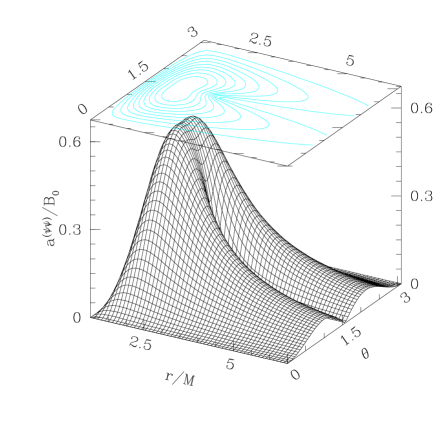
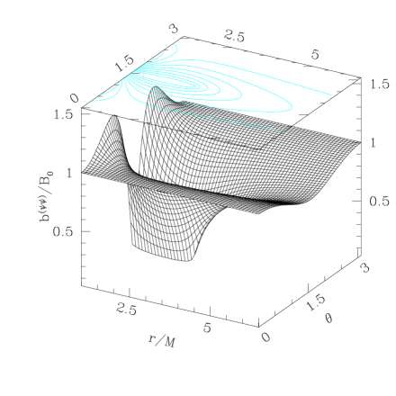
FIG. 1.: The values of the Lorentz invariant “electric” and “magnetic” components of the electromagnetic field surrounding a maximally rotating black hole with the Wald charge, $Q_{\hbox{\rm W}}=2B_{0}J$.

Fig. 1 demonstates that the local strength of the electric field inside the static limit is comparable to that of the applied magnetic field. In regions where $a\sim B_{k}$, the pair-production rate is on the order of $10^{52}$ cm^-3 s^-1 or $L\sim 10^{2}$ (in the rest mass of the particles alone) over the entire spacetime. Clearly, pair production near a rotating black hole must become important for $a\ll\ B_{k}$

A Numerical Results

Summing the pair production rate over a coarse grid yields an an approximate picture of the pair production near rotating black holes. Assuming that the particles reach infinity with the electrostatic injection energy from the region where they appear, gives an estimate of the total pair production luminosity.

FIG. 2.: The pair-production rate and luminosity for a black hole with $a=0.5M$ and $B_{0}=0.27B_{k}$

Fig. 2 depicts the pair-production rate for a black hole with $a=0.5M$ with $B_{0}=0.26B_{k}$. The charge of the black hole deviates from the Wald value with $Q^{\prime}/M^{2}=-0.2B_{k}$ to make the outflow approximately neutral. The total charge of the hole is $Q=0.23Q_{\hbox{\rm W}}$. The pair production is highly concentrated near $r=2.1M$ and a latitude of twenty degrees. This is significantly above the horizon which lies at $r\approx 1.86M$ and slightly outside the static limit. The luminosity is double peaked since the zero potential surface runs through the peak of the pair production.

TABLE I.: Summary of pair-production luminosities from subcritically rotating black holes (numerical results for $L=10^{50}(M/1{\hbox{\rm km}})^{4}$ erg s^-1).

$a/M$	$B_{0}/B_{k}$	$Q^{\prime}/(M^{2}B_{k})$	$Q_{\hbox{\rm W}}/(M^{2}B_{k})$	$W/|W|$
0.1	0.93	-0.17	0.19	0.038
0.2	0.55	-0.20	0.22	0.144
0.3	0.40	-0.21	0.24	-0.218
0.4	0.33	-0.23	0.26	0.217
0.5	0.27	-0.24	0.27	-0.004
0.6	0.23	-0.24	0.28	-0.227
0.7	0.20	-0.24	0.28	0.059
0.8	0.16	-0.21	0.26	-0.085
0.9	0.14	-0.14	0.25	0.276
1.0	0.05	-0.06	0.10	-0.040

Since the pair production is highly localized, especially for slowly rotating black holes, the estimates of the total luminosity are rather sensitive to the resolution of the grid (higher resolutions may yield higher luminosities), and it is difficult to estimate the value of $Q/M^{2}$ required to achieve strict charge neutrality in the outflow.

B Analytic Treatment

Since the pairs are produced in a small region of spacetime around the black hole where $a\ll\ M$, several important simplifications are available. First only the first term in Eq. 22 will be important. Second, the pair-production rate near the peak is approximately Gaussian with characteristic widths in the $r-$ and $\theta-$directions. Third, in this small region where the pair production peaks, spacetime curvature can be neglected. Fourth, in the vicinity of the peak, gradient of the electrostatic potential is constant in magnitude and perpendicular to the zero potential surface, so the passage of the zero potential surface through the peak itself guarantees the charge neutrality of the outflow.

The expansion of the pair production rate about the peak is straightforward and yields,

$$w=w_{\hbox{\rm peak}}\exp\left(-\frac{\pi}{a_{0}}A_{\mu\nu}\Delta r^{\mu}\Delta r^{\nu}\right)$$ (25)

where $\Delta r^{\mu}=r^{\mu}-r_{0}^{\mu}$ and $A_{\mu\nu}$ is positive semidefinite (its nullspace consists of $t-\phi$ plane) and its other eigenvalues are large compared to the characteristic wavenumbers of the blackhole, $1/M$ and 1. The electrostatic injection energy relative to infinity vanishes at the peak and it also may be expanded near the peak as $\epsilon=\epsilon_{;\mu}\Delta r^{\mu}$

Consistent with the approximations mentioned earlier, it is also immediate to integrate the pair production rate and energy flux over space, taking $t={\hbox{\rm Constant}}$ slices,

$$\int\sqrt{-g}wd^{3}x = 4\pi^{2}\sqrt{-g_{0}}\sigma_{1}\sigma_{2}w_{\hbox{\rm peak}}$$ (26)

$$\int\sqrt{-g}|\epsilon|wd^{3}x = \frac{1}{\sqrt{\pi}}\left|\mathaccent 869{A}^{\mu\nu}\epsilon_{;\mu}\right|\int\sqrt{-g}wd^{3}x$$ (27)

where $\mathaccent 869{A}=A^{-1/2}$ and $\sigma_{1}\sigma_{2}$ denotes the product of the nonzero eigenvalues of $\mathaccent 869{A}$.

The energy released (or expended) as the particles travel from where they form to infinity is given by

$$\left.E\right|_{\infty}-\left.E\right|_{\hbox{\rm initial}}=m\left[\sqrt{\frac{\left(\eta_{\mu}\xi^{\mu}\right)^{2}}{\xi_{\mu}\xi^{\mu}}-\eta_{\mu}\eta^{\mu}}-1\right]+\frac{eQ^{\prime}}{2M}\left(\eta_{\mu}\eta^{\mu}-1\right)-\frac{eB_{0}}{2}\eta_{m}u\xi^{\mu}.$$ (28)

$\epsilon$ denotes the component of the energy proportional to the charge of the particle. In Boyer-Lindquist coordinates, this component is given by

$$\epsilon=e\left(\frac{Q^{\prime}}{M^{2}}\frac{M^{2}r}{\Sigma}+B_{0}\frac{2M^{2}r\sin^{2}\theta}{\Sigma}\frac{a}{M}\right).$$ (29)

$\epsilon$ vanishes on the conical surfaces

$$\sin^{2}\theta_{0}=-\frac{1}{2}\frac{Q^{\prime}}{M^{2}}\frac{M}{a}\frac{1}{B_{0}}=-\frac{Q^{\prime}}{Q_{\hbox{\rm W}}}$$ (30)

The component of the energy proportional to the mass of the particle insures that within a thin region bounded by

$$\left|\sin^{2}\theta-\sin^{2}\theta_{0}\right|\approx\frac{r^{2}+a^{2}\cos^{2}\theta_{0}}{Q_{\hbox{\rm W}}r}\frac{m}{|e|}.$$ (31)

particles of neither charge can escape. Near a stellar-mass black hole, this region is on the order of an electron Compton wavelength in thickness; therefore, $m$ may be neglected compared to $e$, leaving only the electrostatic contribution to the energy for consideration. The expansion of $\epsilon$ near the peak yields

$$\epsilon_{;\mu}=\delta_{\mu}^{\theta}\frac{r_{0}\sin 2\theta_{0}}{r_{0}^{2}+a^{2}\cos^{2}\theta_{0}}eQ_{\hbox{\rm W}}.$$ (32)

The location and width of the peak is found by numerically evaluating the pair production rate for a given value of $B_{0}$ and a variable value of $Q^{\prime}/M^{2}$. $Q^{\prime}/M^{2}$ is varied until the peak coincides with the zero $\epsilon$ surface. This procedure works well for $a\lesssim 0.7M$. For larger values of $a$, the peak becomes too broad and splits in two, so the assumptions above are no longer valid. However, since the peak is broad, the direct numerical technique outlined earlier gives reliable results.

Fig. 3 depicts the value of $B_{0}$ to produce a luminosity of $10^{50}\left(M/M_{\odot}\right)^{4}$ erg s^-1 as a function of $a$ for $0.01\leq a\leq 0.81$ and the mean value of $\gamma$ for the primary particles.

FIG. 3.: The left panel shows the strength of imposed magnetic field to produce a luminosity of $10^{50}(M/M_{\odot})^{4}$ erg s^-1 for a given value of $a/M$. The solid squares give the numerical results. The solid line in right panel traces the mean value of $\gamma$ of the primary particles and the dashed line traces the approximate formula Eq. 34.

The value of $B_{0}$ is well fit by a power-law such that $B_{0}=B_{c}(10a/M)^{-4/5}$. The luminosity increases exponentially with $a$ and superexponentially with $B_{0}$. A convenient fitting formula is

$$\log_{10}\left(\frac{L}{10^{30}{\hbox{\rm erg s}}^{-1}}\right)=200\frac{a}{M}\left(\frac{B}{B_{c}}\right)^{5/4}+4\log_{10}\left(\frac{M}{M_{\odot}}\right).$$ (33)

The location of the pair production and typical escape energies of the pairs also changes with the angular momentum of the hole. Fig. 4 depicts the colatitude of the peak and the radius of the peak. A comparison of the right panel of Fig. 3 with the left panel Fig. 4 verifies that the typical value of $\gamma$ depends rather simply on the colatitude of the peak and $a$ through Eq. 27. For small values of $a$ ($a\lesssim 0.6M$), one eigenvector of the matrix $\mathaccent 869{A}$ points in the $\theta$-direction, the value of $\gamma$ is approximately given by

$$\gamma\approx\frac{2\sigma_{\theta}}{\sqrt{\pi}}\frac{ar_{0}\sin 2\theta_{0}}{r_{0}^{2}+a^{2}\cos^{2}\theta_{0}}\frac{B_{0}}{B_{c}}\frac{M}{\hbar/mc}$$ (34)

where $\sigma_{\theta}\approx 0.055$. For larger values of $a$, the eigenvectors rotate away from the $r-$ and $\theta-$directions, and the approximation is poorer.

The pair production peaks near the equatorial plane for small values of $a$ and moves toward the poles as $a$ increases. Meanwhile the peak remains outside the static limit until $a\approx 0.7M$ then crosses the static limit and moves toward the horizon (c.f. Fig. 4). Fig. 5 illustrates how the analytic treatment becomes unreliable for high values of $a$. As $a$ approaches $M$, the peak becomes broad, and the assumptions which support the analytic treatment become invalid.

FIG. 4.: The position of the peak of the pair production as a function of the angular momentum of the black hole. In the right panel, the radius of the peak is traced by the solid line, the radius of the horizon by the short-dashed line, and the radius of the static limit at the latitude of the peak by the long-dashed line.

FIG. 5.: The position and principal axes of the peak. For $a=0.1M,0.72M$ and $0.81M$. The peak crosses the static limit at $a\approx 0.727M$.

For $a>0.735M$, the value of $I$ on the horizon near the spin axis becomes negative since $Q^{\prime}/M^{2}<(-4+2\sqrt{3})B_{0}$; consequently, for larger values of $a$ pairs are produced both in the main peak and in the polar regions near the horizon. This polar component does not contribute significantly to the total pair production until $a\sim 0.8M$ Fig. 6 depicts the net pair production rate near a black hole with $a=0.8M$. The main peak is quite broad with positrons escaping nearer to the equator and electrons at higher latitudes. The horizon component of the pair production consists exclusively of electrons. Although locally the rate is quite large, only a small volume is active, so its total contribution is small.

FIG. 6.: The left panel shows the net pair production rate for $a=0.8M$ with $B_{0}=0.165B_{c}$ and $Q^{\prime}/M^{2}=-0.211B_{c}$. The right panel shows the pair-production luminosity.

IV Conclusions

The vacuum surrounding a magnetized, rotating black hole is unstable to pair production if the imposed field approaches $B_{k}=m^{2}c^{3}/(e\hbar)\approx 4.4\times 10^{13}$ G $\approx 1.3\times 10^{-11}$ cm^-1. If the mass of the black hole $M$ is much less then $10^{11}$ cm or $10^{6}$ M_⊙, the field does not contribute significantly to spacetime curvature. For the process as outlined to operate, the vicinity of the black hole must initially be free of charge, so the large potential gap and strong electric field remain stable for subcritical fields; therefore, one would not expect this simple description to apply astrophysically.

Adapting the model of Goldreich and Julian [6] to the case of a rotating black hole provides an estimate of the charge density necessary to short the electric field. Two natural definitions of the angular velocity are that of the zero-angular-momentum frame at the horizon and at the peak of the pair production. Both choices result in the constraint that the electron density must exceed $2-4\times 10^{15}$ cm^-3 for a one-solar-mass black hole to short the electric field. This is several orders of magnitude larger than the Goldreich-Julian density typical for rotating neutron stars. Even if the initial charge density does exceed this value, the vacuum case provides important insights.

Van Putten’s estimates for the pair production luminosity fall short of those calculated here by several orders of magnitude [8, 9] and depend differently on the mass of the black hole and the strength of the magnetic field imposed. Since for weak fields the luminosity depends superexponentially on the imposed magnetic field, agreement can be achieved in the gross properties of the models by slightly varying the magnetic field strength. For supercritical fields the pair production rate locally increases as $B_{0}^{2}$, and the electrostatic injection energy, $\epsilon$, is proportional to $B_{0}M$; consequently, the total luminosity increases as $B_{0}^{3}M^{4}$ – van Putten argues that the total luminosity increases as $B_{0}^{2}M^{2}$. Reconciling these differences is difficult as this report and van Putten’s work treat the underlying physical processes differently.

Some natural extensions to this work are a treatment of the back reaction of the outflow on the spin of the black hole and the source of the external magnetic field. By including a more realistic description of the magnetic field far from the hole which would likely include a model for its source, the beaming of the relativistic jet could be determined. These developments would constrain the duration of the emission, the nature of its onset and its possible modulation. The pairs will naturally produce secondary particles as they travel along the curved magnetic field lines. These secondaries, the primaries or previously present material could form a magnetosphere around the black hole, causing the electromagnetic field to evolve toward a force-free configuration (e.g. [20]).

Rotating black holes coupled to strong magnetic fields naturally produce a highly relativisitic, columnated outflow with a total luminosity which can easily exceed $10^{50}$ erg/s. The electrons and positrons are initially separated. For $a\gtrsim 0.8M$, if the applied field is parallel (antiparallel) to the angular momentum of the black hole, electrons (positrons) will escape from polar regions near the horizon from a region near the equatorial plane within the static limit. Positrons (electrons) escape only from the equatorial region. For small values of $a$, both electrons and positrons escape from a small region outside the static limit whose latitude depends on the value of $a$.

REFERENCES

- [1] V. V. Usov, Nature (London) 357, 472 (1992).
- [2] E. G. Blackman and I. Yi, ApJ 498, L31 (1998).
- [3] P. Meszaros and M. J. Rees, ApJ 482, L29 (1997).
- [4] B. Paczynski, ApJ 494, L45 (1998).
- [5] H. K. Lee, R. A. M. J. Wijers, and G. E. Brown, Phys. Rep. 325, 83 (2000).
- [6] P. Goldreich and W. H. Julian, ApJ 157, 869 (1969).
- [7] R. D. Blandford and R. L. Znajek, MNRAS 179, 433 (1977).
- [8] M. H. P. M. van Putten, Phys. Rev. Lett. (2000), submitted, astro-ph/9911396.
- [9] M. H. P. M. van Putten, in Explosive Phenomena in Astrophysics of Compact Objects, edited by C.-H. Lee, M. Rho, I. Yi, and H. K. Lee (AIP, Woodbury, New York, 2000).
- [10] G. W. Gibbons, Comm. Math. Phys. 44, 245 (1975).
- [11] G. W. Gibbons, MNRAS 177, 37P (1976).
- [12] R. M. Wald, Phys. Rev. D 10, 1680 (1974).
- [13] L. D. Landau and E. M. Lifshitz, The Classical Theory of Fields, fourth ed. (Pergamon, Oxford, 1987).
- [14] S. W. Hawking and G. F. R. Ellis, The Large Scale Structure of Space-Time (Cambridge, Cambridge, 1973).
- [15] W. Heisenberg and H. Euler, Z. Physik 98, 714 (1936).
- [16] C. Itzykson and J.-B. Zuber, Quantum Field Theory (McGraw-Hill, New York, 1980).
- [17] J. S. Heyl and L. Hernquist, Phys. Rev. D 55, 2449 (1997).
- [18] J. K. Daugherty and I. Lerche, Phys. Rev. D14, 340 (1976).
- [19] J. Schwinger, Physical Review 82, 664 (1951).
- [20] H. K. Lee, C. H. Lee, and M. H. van Putten, astro-ph/0009239 (unpublished).