Regression Depth and Center Points

Abstract

We show that, for any set of $n$ points in $d$ dimensions, there exists a hyperplane with regression depth at least $\lceil n/(d+1)\rceil$, as had been conjectured by Rousseeuw and Hubert. Dually, for any arrangement of $n$ hyperplanes in $d$ dimensions there exists a point that cannot escape to infinity without crossing at least $\lceil n/(d+1)\rceil$ hyperplanes. We also apply our approach to related questions on the existence of partitions of the data into subsets such that a common plane has nonzero regression depth in each subset, and to the computational complexity of regression depth problems.

1 Introduction

Robust statistics [13, 32] has attracted much attention recently within the computational geometry community due to the natural geometric formulation of many of its problems. In contrast to least-squares regression, in which measurement error is assumed to be normally distributed, robust estimators allow some of the data to be affected by completely arbitrary errors. Researchers in this crossover area have developed algorithms for problems such as center point construction [6, 16, 24], slope selection [3, 7, 10, 18, 21], and the least median of squares regression method [11, 22] proposed by Rousseeuw [28].

Recently, Rousseeuw and Hubert [15, 31, 30] introduced regression depth as a quality measure for robust linear regression: in statistical terminology, the regression depth of a hyperplane $H$ is the smallest number of residuals that need to change sign to make $H$ a nonfit. This definition has convenient statistical properties such as invariance under affine transformations; hyperplanes with high regression depth behave well in general error models, including skewed or heteroskedastic error distributions.

Geometrically, the regression depth of a hyperplane is the minimum number of points intersected by the hyperplane as it undergoes any continuous motion taking it from its initial position to vertical. In the dual setting of hyperplane arrangements, the undirected depth of a point in an arrangement is the minimum number of hyperplanes touched by or parallel to a ray originating at the point. Standard techniques of projective duality transform any statement about regression depth to a mathematically equivalent statement about undirected depth and vice versa.

Rousseeuw and Hubert [31, 30] showed that for any $n$ and $d$ there exist sets of $n$ points in $d$ dimensions such that no hyperplane has regression depth larger than $\lceil n/(d+1)\rceil$. For $d=2$, they found a simple linear-time construction which achieves the optimal $\lceil n/3\rceil$ bound. These facts, together with an analogy to center points (points such that any halfspace containing them also contains many data points), led to the following conjectures:

Conjecture 1 (Rousseeuw and Hubert)

For any $d$-dimensional set of $n$ points there exists a hyperplane having regression depth $\lceil n/(d+1)\rceil$.

Conjecture 2 (Rousseeuw and Hubert)

For any point set there exists a partition into $\lceil n/(d+1)\rceil$ subsets and a hyperplane that has nonzero regression depth in each subset.

Steiger and Wenger [34] made some progress on Conjectures 1 and 2: they show that any point set can be partitioned into $c_{d}n$ subsets, where $c_{d}$ is a constant depending on the dimension $d$, such that there exists a hyperplane having nonzero regression depth in each subset. Note that such a hyperplane must have regression depth at least $c_{d}n$. Their value $c_{d}$ is not stated explicitly, however it appears to be quite small: roughly $1/(6^{d^{2}}(d+1))$.

Questions of computational efficiency of problems related to regression depth have also been studied. Rousseeuw and Struyf [33] described algorithms for testing the regression depth of a given hyperplane. The same paper also considers algorithms for testing the location depth of a point (its quality as a center point). One can find the hyperplane of greatest regression depth for a given point set in time $O(n^{d})$ by a breadth first search of the dual hyperplane arrangement; standard $\epsilon$-cutting methods [23] can be used to develop a linear-time approximation algorithm that finds a hyperplane with regression depth within a factor $(1-\epsilon)$ of the optimum in any fixed dimension. For bivariate data, van Kreveld, Mitchell, Rousseeuw, Sharir, Snoeyink, and Speckmann found an algorithm for finding the optimum regression line in time $O(n\mathop{\rm log}^{2}n)$ [19], recently improved to $O(n\mathop{\rm log}n)$ by Langerman and Steiger [20].

Our main result is to prove the truth of Conjecture 1. We do this by finding a common generalization of location depth and regression depth that formalizes the analogy between these two concepts: the crossing distance between a point and a plane is the smallest number of sites crossed by the plane in any continuous motion from its initial location to a location incident to the point. The location depth of a point is just its crossing distance from the plane at infinity, and the regression depth of a plane is just its crossing distance from the point at vertical infinity. We then prove the conjecture by using Brouwer’s fixed point theorem to find a projective transformation that maps the point at vertical infinity to a center point of the transformed sites; the inverse transformation maps the plane at infinity to a deep plane.

We also improve the partial result of Steiger and Wenger on Conjecture 2: we show that one can always partition a data set into $\lceil n/d(d+1)\rceil$ subsets with a hyperplane having nonzero regression depth in each subset. We further improve this to $\lfloor(n+1)/6\rfloor$ for $d=3$. Our technique of projective transformation also sheds some light on issues of computational complexity: the two problems of testing regression depth and location depth considered by Rousseeuw and Struyf are in fact computationally equivalent. Known NP-hardness results for center points then lead to the observation that testing regression depth is NP-hard for data sets of unbounded dimension.

2 Overview of the Proof

Before we begin the detailed proof, we describe our proof strategy and outline some of the points of difficulty.

As discussed above, it is sufficient to find a projective transformation such that the image of the point at vertical infinity is a center point of the transformed set. Equivalently, the point at vertical infinity should have large crossing number with the plane at infinity of the transformed set, so the inverse image of this plane has high regression depth.

To find such a transformation, we view our space $\Bbb R^{d}$ as being embedded in $\Bbb R^{d+1}$, tangent to a $d$-sphere, use central projection to lift the points in $\Bbb R^{d}$ to pairs of points on the $d$-sphere, and use central projection again to flatten them onto a copy of $\Bbb R^{d}$ tangent at a different point $p$ of the $d$-sphere. In this way, we get a different transformation for each point $p$ of the sphere. For each such transformation we consider a point $f(p)$ on the sphere, found by computing a center point of the transformed point set and lifting it back to the sphere again. Note that $f(p)$ will automatically be in the same hemisphere as $p$.

By the Brouwer fixed point theorem, any continuous function on the sphere that maps points to the same hemisphere must be surjective (Corollary 1). If $f$ is surjective, there exists a $p$ for which $f(p)$ is the lifted image of the point at vertical infinity, giving us the transformation we want.

However, there are some technical difficulties. As sketched above, $f(p)$ is not continuous, for two reasons: first, there may be a large set of center points, and it is difficult to pick a single one in a continuous way. Second, and more importantly, as we move $p$ continuously on the sphere, the set of center points changes drastically at those times when $p$ makes an angle of $\pi/2$ with a member of our point set, so that the transformed image of the point moves out to infinity in one direction and comes back in another.

To make the set of center points change more continuously, we approximate the lifted point set on the sphere by a smooth measure. It is not hard to generalize the concept of location depth to measures, and to extend the proof of the existence of center points to this setting (Lemma 6), but there still may not exist a unique center point. To chose a single continuously varying point $f(p)$, we use the centroid of the set of points with location depth $\geq\lceil n/(d+1)\rceil-\epsilon$. Proving that this defines a continuous function involves defining an appropriate metric on a space of measures (Lemma 1), representing $f(p)$ as a composition of functions to and from this space of measures, and using the fact that the set of points used to define $f(p)$ is convex with nonempty interior (Lemma 7) together with smoothness assumptions on the measure to show that the terms in this composition are each continuous (Lemmas 2, 3, and 8).

If we now apply the same Brouwer fixed point argument, we get a transformation that takes the point at vertical infinity to a point with location depth $\lceil n/(d+1)\rceil-\epsilon$. This gives us a hyperplane $H$ with high, but not quite high enough, regression depth in the measure approximating our point set. To finish the argument, and prove the existence of a hyperplane with high regression depth, we show that there exists an $\epsilon$, and a measure approximating the point set and having the required smoothness properties, such that we can find a hyperplane near $H$ with the stated bound on regression depth for the original point set (Lemmas 4 and 5).

3 Geometric Preliminaries

3.1 Projective Geometry

Although Rousseeuw and Hubert’s conjectures are defined purely in terms of Euclidean geometry, our proof fits most naturally in the context of projective geometry. We briefly review this geometry here, since standard textbooks (e.g. [8]) concentrate primarily on the planar version, and we need higher dimensions.

Perhaps the simplest way to view $d$-dimensional projective space is as a renaming of Euclidean objects one dimension higher. Call a projective point a line through the origin of $(d+1)$-dimensional Euclidean space, and a projective hyperplane a hyperplane containing the origin of the same $(d+1)$-dimensional space. Then these projective points and hyperplanes satisfy properties resembling those of $d$-dimensional Euclidean points and hyperplanes. Indeed, one can embed Euclidean space into this projective space, in the following way: embed a copy of $d$-dimensional Euclidean space as a hyperplane in $(d+1)$-dimensional space, avoiding the origin (so this hyperplane is not a projective hyperplane). Then through any point of the $d$-dimensional space, one can draw a unique line through it and the origin; that is, the Euclidean point corresponds to a unique projective point. Similarly, each hyperplane in the $d$-dimensional space corresponds to a unique projective hyperplane. However, there is one projective hyperplane, and there are many projective points, that do not come from Euclidean points and hyperplanes in this way; namely the $(d+1)$-dimensional hyperplane through the origin parallel to the $d$-dimensional space, and all $(d+1)$-dimensional lines contained in that hyperplane. We call these projective objects points at infinity and the hyperplane at infinity. In particular, all vertical Euclidean hyperplanes, when extended to the projective space, meet in a single projective point, which we call the point at vertical infinity ($\hat{\infty}$ for short).

A projective transformation is a map from one projective space to another of the same dimension that takes points to points, hyperplanes to hyperplanes, and preserves point-hyperplane incidences. These include (extensions of) the usual Euclidean affine transformations, but also some other transformations in which infinite points are mapped to finite points or vice versa.

3.2 Central Projection

Central projection is a correspondence from hyperplanes to spheres closely related to the extension described above from Euclidean to projective spaces.

Suppose we are given a $d$-dimensional hyperplane $E$ in $(d+1)$-dimensional space, tangent to a $d$-sphere $S$. Then given any set $X$ of $n$ point sites in $E$, we can lift this set to a set $\breve{X}$ of $2n$ point sites on $S$, as follows: draw a line through each site and the center of $S$; this line intersects $S$ in two points; place a site at both points. Conversely, given any function $f:S\mapsto\Bbb R$, we can “flatten” it to a function $\bar{f}:E\mapsto\Bbb R$, as follows: for each point $x$ in $E$, draw a line through $x$ and the center of $S$; this line intersects $S$ in two points $y$ and $z$, one of which (say $y$) is in the open hemisphere of $S$ centered on the point of tangency; let $\bar{f}(x)=f(y)$. In either case we define the pole of the projection to be the common point of tangency between the hyperplane and the sphere.

The effect of lifting a hyperplane to a sphere and then flattening the sphere to a different hyperplane can be viewed as a projective transformation: if one places the origin at the sphere center, the operations of drawing a line through a point, as used in both lifting and flattening, are exactly the way we embedded Euclidean space in projective space as described earlier. The two different hyperplanes simply form different Euclidean views of the same projective space.

If one is given a Euclidean space (without a tangent sphere) the act of lifting to a sphere requires an arbitrary choice: where to put the tangent sphere. Similarly if one is given a sphere (without a tangent hyperplane) the act of flattening to a hyperplane requires a choice of where to put the pole, and is completely determined once that choice is made. In our proof, we will find a projective transformation from one space to another by choosing arbitrarily a tangent sphere to our initial space, and then considering all possible pole locations on that sphere.

3.3 Measure Theory

A measure on a topological space $X$ is just a function $m$ from a family of subsets of $X$ (which must be closed under the complement and countable union operations, and include all the open and closed subsets) to nonnegative real numbers, satisfying the property of countable additivity: if a set $S$ is a disjoint union of countably many measurable subsets, then the measures of those subsets must form a convergent series summing to $m(S)$. We restrict our attention to measures for which the measurable sets are just the Borel sets: sets that can be formed from open sets by a sequence of complement and countable union operations.

The usual Euclidean volume (Lebesgue measure) in $\Bbb R^{d}$ is not quite a measure under our definition, because we want even the whole space to have finite measure, but it is a measure on any restriction of $\Bbb R^{d}$ to a bounded subset, or on the surface of a sphere. One can also define a discrete measure from a set of point sites, in which the measure of a set $S$ is simply the number of sites it contains.

Any measure $m$ on a sphere can be flattened to a measure $\bar{m}$ on Euclidean space: given a set $S$ in Euclidean space, let $\breve{S}$ be the copy of $S$ lifted by central projection to a subset of the open hemisphere centered on the pole of projection, and let $\bar{m}(S)=m(\breve{S})$.

We define a smooth measure $m$ on the $d$-sphere to be one for which there is a bound $b$ such that, for any set $S$, $m(S)$ is at most $b$ times the Lebesgue measure. We define a smooth measure on $\Bbb R^{d}$ to be one formed by flattening a smooth measure on the sphere. (This is stronger than simply requiring a bounded ratio between the measure and Lebesgue measure in $\Bbb R^{d}$.) Since any Lebesgue measurable set is the difference of a countable intersection of open sets with a measure-zero set [25, Theorem 3.15], a smooth measure is completely determined by its behavior on open sets. We define a measure to be nowhere zero if all open sets have nonzero measure; note that we do not require the measure of the open sets to be bounded below by a constant times their Lebesgue measure.

For any smooth measures $m_{1}$ and $m_{2}$ on the sphere or $\Bbb R^{d}$ define the distance between $m_{1}$ and $m_{2}$ to be the supremum of $|m_{1}(S)-m_{2}(S)|$ where $S$ ranges over all convex subsets of $X$ (convex subsets of the sphere are defined to be sets that can be flattened to a convex subset of $\Bbb R^{d}$).

Lemma 1

The distance defined above is a metric on the space of smooth measures.

Proof: The distance is clearly symmetric. Any open set can be decomposed into a union of countably many convex sets, and we can use inclusion-exclusion to express its measure as a series each term of which is the measure of a convex set; therefore any two distinct smooth measures have nonzero distance. The triangle inequality is satisfied separately by the values $|m_{1}(S)-m_{2}(S)|$ for each $S$, so it is satisfied by the overall distance as well.

Lemma 2

Let $m$ be a smooth measure on a sphere, and let $R$ be the group of rotations of the sphere. Define the measure $m_{\rho}(S)=m(\rho(S))$ for any $\rho\in R$. Then the map from $\rho$ to $m_{\rho}$ is a continuous function from $R$ to the space of smooth measures.

Proof: We need to show that for any $\rho$ and $\epsilon$ we can find a $\delta$ such that all rotations within $\delta$ of $\rho$ are mapped to a measure within $\epsilon$ of $m_{\rho}$. By symmetry of the space of rotations, we can assume $\rho$ is the identity.

For any set $S$ and rotation $\theta$, $|m(S)-m(\theta(S))|\leq m(S\oplus\theta(S))=O(b|\theta|L)$, where $b$ is the bound on $m$ in terms of Lebesgue measure assumed in the definition of smoothness and $L$ is the Lebesgue measure of the boundary of $S$. For any convex set, $L$ is bounded independently of $S$ by the measure of the equator of the sphere, so if we choose $\delta=O(1/b)$, any rotation amount smaller than $\delta$ will have $|m(S)-m_{\rho}(S)|<\epsilon$ as desired.

Lemma 3

Flattening a sphere to a hyperplane (with a fixed pole of projection) induces a continuous map from the space of smooth measures on the sphere to the space of smooth measures on $\Bbb R^{d}$.

Proof: Flattening can only decrease the distance between two measures, since the flattened distance is of the same form (a supremum of values $|m_{1}(S)-m_{2}(S)|$) but with fewer choices for $S$ (only those convex subsets of the sphere that are contained in a particular open hemisphere).

3.4 Smoothing and Sharpening

In order to avoid complicated limit arguments, we will approximate the discrete measure of a set of sites by a single smooth measure, carefully chosen so that we can translate halfspaces in one measure to halfspaces in the other in a way that preserves the measure of the cuts appropriately. As a notational convention, we will use accented letters like $H^{\prime}$ to refer to objects related to the discrete measure, and unaccented letters like $H$ to refer to the corresponding objects for the smooth measure.

Any pair of hyperplanes in a projective space divides the space into two subsets; we define a double wedge to be the closure of any such subset. In particular a Euclidean halfspace is a special case of a double wedge in which one of the hyperplanes is the hyperplane at infinity. Given a set of sites, we say that two hyperplanes are combinatorially equivalent if they bound a double wedge that has no sites in its interior. Note that this is not really an equivalence relation because of the possibility of sites on the boundary of the wedge.

The proofs of some lemmas in this section rely on projective duality: in any projective space, one can find a correspondence between it and a dual space of the same dimension, in which each point $p$ corresponds to a dual hyperplane $p^{*}$, and each hyperplane $H$ corresponds to a dual point $H^{*}$, such that $p$ is incident to $H$ if and only if $p^{*}$ is incident to $H^{*}$. Note that, under this correspondence, the set of hyperplanes passing within distance $\delta$ of point $p$ is transformed into a set of points within some neighborhood of hyperplane $p^{*}$.

Lemma 4

For any finite set of sites in $\Bbb R^{d}$, there exists a $\delta$ such that any hyperplane $H$ can be replaced by a combinatorially equivalent hyperplane $H^{\prime}$, such that $H^{\prime}$ is incident to all sites within distance $\delta$ of $H$.

Proof: Let $\delta$ be smaller than half the height of any nondegenerate simplex formed by $d+1$ points. For any $H$, let $S_{0}$ denote the set of sites within distance $\delta$ of $H$; then $S_{0}$ must be coplanar. Let $H_{0}$ be any plane incident to all sites in $S_{0}$, and continuously rotate $H$ towards $H_{0}$ around an axis where the two hyperplanes intersect. (This motion is easier to understand in the dual: it is just motion along a straight line segment from $H^{*}$ to $H_{0}^{*}$.) Note that with such a motion, the distance from $H$ to any point of $H_{0}$, and in particular to any of the sites in $S_{0}$, is monotonically decreasing, so no site can leave set $S_{0}$. However, $H$ may move to within distance $\delta$ of some site $x$ outside of $S_{0}$; if this happens, we stop moving towards $H_{0}$, form set $S_{1}=S_{0}\cup\{x\}$, find a plane $H_{1}$ incident to all points in $S_{1}$, continue rotating towards $H_{1}$, etc. Since there are only finitely many sites, this process must eventually terminate with a plane $H^{\prime}$ incident to all sites crossed by the motion of $H$; therefore there are no sites interior to the double wedge defined by $H$ and $H^{\prime}$.

Lemma 5

For any finite set of sites in $\Bbb R^{d}$, there exists a $\delta$ such that any hyperplane $H^{\prime}$ can be replaced by a combinatorially equivalent hyperplane $H$, such that $H$ is at distance at least $\delta$ from any site.

Proof: Form the hyperplane arrangement dual to the set of sites; choose $\delta$ small enough that each cell of the arrangement has a point not covered by any $\delta$-neighborhood of any hyperplane. For any $H$, let ${H^{\prime}}^{*}$ be an uncovered point in a cell containing $H^{*}$, and let $H^{\prime}$ be the hyperplane dual to ${H^{\prime}}^{*}$.

We will apply Lemma 4 to the original sites, and Lemma 5 to their vertical projections.

3.5 Center Points

If we are given a set of point sites in $\Bbb R^{d}$, the location depth (also known as Tukey depth) of a point $x$ (which may not necessarily be itself a site) is defined to be the minimum, over all projections $\pi:\Bbb R^{d}\mapsto\Bbb R$, of the number of sites with $\pi(s)\leq\pi(x)$. Equivalently, it is the minimum number of sites contained in any closed halfspace containing $x$. (The halfspace corresponding to projection $\pi$ is $\{y:\pi(y)\leq\pi(x)\}$.)

More generally, if $m$ is a measure on $\Bbb R^{d}$, we define the the location depth of $x$ to be the minimum measure of any halfspace containing $x$. Note that for any $D$ the set of points with location depth at least $D$ is an intersection of closed halfspaces, and is therefore closed and convex.

A Tukey median is a point with maximum location depth. A center point is a point with location depth at least $m(\Bbb R^{d})/(d+1)$. As is well known [1, 9, 26] a center point exists for any discrete measure; equivalently, any Tukey median is a center point. We extend this to arbitrary measures using the main idea from one proof of the discrete case: applying Helly’s theorem to a family of high-measure sets.

Lemma 6

For any measure $m$ on $\Bbb R^{d}$, there exists a point with location depth at least $m(\Bbb R^{d})/(d+1)$.

Proof: For any positive integer $i$, let $\epsilon=1/i$, let $X$ be a compact convex set with measure at least $(1-\epsilon)m(\Bbb R^{d})$ (such a set always exists since $\Bbb R^{d}$ is a countable union of nested convex bounded sets) and consider the family $F$ of compact convex subsets of $X$ with measure at least $(d/(d+1)+\epsilon)m(\Bbb R^{d})$. The measure of the complement in $X$ of any set in $F$ is at most $m(X)/(d+1)-\epsilon m(R^{d})$, so the intersection of any $(d+1)$-tuple of sets in $F$ must be nonempty. By Helly’s theorem [14, 9] there is a point $x_{i}$ contained in all members of $F$.

If any open halfspace disjoint from $x_{i}$ has measure larger than $(d/(d+1)+2\epsilon)m(\Bbb R^{d})$, some closed halfspace contained in it also has measure larger than $(d/(d+1)+2\epsilon)m(\Bbb R^{d})$, and would intersect $X$ in a compact convex set of measure larger than $(d/(d+1)+\epsilon)m(\Bbb R^{d})$, contradicting the assumption that $x_{i}$ is in the intersection of all such sets. Therefore, $x_{i}$ has location depth at least $(1/(d+1)-2\epsilon)m(\Bbb R^{d})$.

Since we can make $\epsilon$ as small as we wish (and since all points with location depth at least $\epsilon m(\Bbb R^{d})$ must be contained in the compact set $X$), we can find a cluster point of the points $x_{i}$, and this cluster point must have location depth at least $m(\Bbb R^{d})/(d+1)$.

Define an $\epsilon$-center point to be a point with location depth at least $m(\Bbb R^{d})/(d+1)-\epsilon$.

Lemma 7

For any smooth measure $m$ in $\Bbb R^{d}$, and any sufficiently small $\epsilon$, the set of $\epsilon$-center points is compact and has nonempty interior.

Proof: Let $m$ be formed by flattening a smooth measure $\breve{m}$ on the sphere, and let $c$ be a center point of $m$. For any $\epsilon$ there exists a $\delta$ for which any infinite strip of width $\delta$ containing $c$ has measure at most $\epsilon$ (since the lift of such a strip is a narrow wedge of the sphere). Therefore, the points in an open ball of radius $\delta$ around $c$ are all $\epsilon$-center points.

Let $\epsilon$ be small enough that the location depth of an $\epsilon$-center point is bounded away from zero. The set of $\epsilon$-center points is clearly closed by its definition. To show that the set is bounded, note that for any $\delta$ one can find a neighborhood of the equator of the sphere with measure at most $\epsilon$; for any point $x$ in this neighborhood, one can find a halfspace in $\Bbb R^{d}$ containing the point that is a subset of the flattening of this neighborhood, and that therefore has too small a measure for $x$ to be an $\epsilon$-center point. The complement of this flattened neighborhood is a bounded region of $\Bbb R^{d}$.

Define the $\epsilon$-trimmed mean of a measure $m$ to be the centroid of its set of $\epsilon$-center points.

Lemma 8

For any sufficiently small $\epsilon>0$, the map from measures to $\epsilon$-trimmed means defines a continuous function from nowhere zero smooth measures to $\Bbb R^{d}$.

Proof: Let $m$ be a smooth nowhere zero measure, and $K$ its set of $\epsilon$-center points. Then $K$ is an intersection of closed halfspaces, so any point $x$ outside $K$ is contained in an open halfspace $H$ tangent to $K$ and having measure $m(\Bbb R^{d})/(d+1)-\epsilon$. Let $S$ be the infinite slab bounded on one side by the boundary of $H$, and on the other side by a hyperplane through $x$. The halfspace on the other side of this slab from $K$ has measure $m(\Bbb R^{d})/(d+1)-\epsilon-m(S)$, and $x$ can only become an $\epsilon$-center point of a measure with distance at least $m(S)$ from $m$. In other words, for any $x$ outside $K$ there is a $\delta=m(S)$ such that measures within distance $\delta$ of $m$ do not have $x$ in their set of $\epsilon$-center points.

For any $y$ interior to $K$, let $S_{i}$ (for $i=1\ldots 2^{d}$) be the intersections with $K$ of a system of orthants centered at $y$. Then any halfspace containing $y$ can be decomposed into a slab containing one of the $S_{i}$ and a smaller halfspace containing a boundary point of $K$; therefore by a similar argument to the one above, there is a $\delta=\mathop{\rm min}\{m(S_{i})\}$ such that all measures within distance $\delta$ of $m$ have $y$ in their set of $\epsilon$-center points.

Thus an arbitrarily small change to the measure can only change the set of $\epsilon$-center points in an arbitrarily small region near the boundary of $K$, which can only make the centroid of $K$ change by an arbitrarily small amount.

3.6 Brouwer’s Theorem and Functions on Spheres

The following well-known fact about functions on spheres is a simple consequence of the Brouwer fixed point theorem, that any continuous function from a closed topological disk to itself has a fixed point [4, 5].

Lemma 9

Let $f$ be a continuous non-surjective function from a $d$-sphere $S$ to itself. Then $f$ has a fixed point.

Proof: Since $f$ is non-surjective, there is a point $x$ not covered by $f$. Since $f$ is continuous, it avoids an open neighborhood $N$ of $x$. Then the restriction of $f$ to $S\setminus N$ is a continuous map from a closed disk to itself, and hence by the Brouwer fixed point theorem has a fixed point.

Corollary 1

Let $f$ be a continuous function from a $d$-sphere to itself such that for all $x$, $f(x)\neq-x$. Then $f$ is surjective.

Proof: Apply the lemma to $-f$.

4 The Proof

If $m$ is a measure on a projective space, we define the crossing distance $\chi_{m}(x,H)$ between a point $x$ and a hyperplane $H$ to be the minimum measure of any double wedge where one boundary hyperplane is $H$ and the other contains $x$. Intuitively, if $m$ is a discrete measure coming from a set of point sites, $\chi$ measures the number of points that must be crossed by $H$ in any continuous motion of hyperplanes that moves $H$ until it touches $x$.

Then, the location depth of a point $x$ is simply $\chi_{m}(x,\infty)$ where $\infty$ denotes the hyperplane at infinity. Conjecture 1 can be rephrased as asking for a hyperplane $H$ such that $\chi_{m}(\hat{\infty},H)$ is large. Therefore, location depth and regression depth are both special cases of crossing distance.

Since crossing distance is defined purely projectively, it is preserved by any projective transformation. Thus if we find a hyperplane with high regression depth, performing a projective transformation that takes it to the hyperplane at infinity will also take the point at vertical infinity to a center point. Conversely, if we can find a projective transformation that takes the point at vertical infinity to a center point, the preimage of the hyperplane at infinity must have high regression depth.

Our proof of Conjecture 1, below, finds such a transformation as a composition of two central projections. The idea of the proof is very simple: lift the sites to a sphere, flatten the sphere at a pole, compute the center point of the flattened points, and use Corollary 1 to show that this map from poles to center points covers $\hat{\infty}$. All of the technical complication in the proof arises from our need to force “the center point” to be unique and the map to be continuous, which we do by approximating the points with smooth measures and using $\epsilon$-trimmed means of these measures.

Theorem 1

For any $n$ points in $\Bbb R^{d}$ there exists a hyperplane having regression depth $\lceil n/(d+1)\rceil$.

Proof: Use central projection with an arbitrary fixed choice of tangent sphere to lift the sites to a set of $2n$ points on a sphere. The extension of this lifting map to the projective space lifts the point at vertical infinity to two points on the sphere; choose one of these two arbitrarily and call it $\hat{\infty}$.

Let $\delta$ be small enough that we can apply Lemma 4 to the sites and Lemma 5 to the vertical projection of the sites. Let $\epsilon=1/3(d+1)$. Choose a smooth nowhere zero measure $m$ such that the measure of any hemisphere is $n$, the $\delta$-radius ball around any site has measure at most one, and the total measure of the set of points farther than $\delta$ from any site is at most $\epsilon$.

Define the function $c(x)$ from the sphere to itself as follows: let $\bar{m}(x)$ be the measure formed by flattening $m$ at pole $x$, let $\bar{c}(x)$ be the $\epsilon$-trimmed mean of $\bar{m}(x)$, and use central projection to lift $\bar{c}(x)$ to a point $c(x)$ in the open hemisphere centered on $x$. By Lemmas 2, 3, and 8, $c$ is continuous, and clearly $c$ has no point for which $c(x)=-x$. Then by Corollary 1, $c$ is surjective, so we can find a point $p=c^{-1}(\hat{\infty})$ such that flattening the sphere tangent to $p$ maps $\hat{\infty}$ to the $\epsilon$-trimmed mean of $\bar{m}(p)$.

Let $H$ denote the hyperplane at infinity with respect to $p$. Use Lemma 4 to sharpen $H$ to a hyperplane $H^{\prime}$ incident to all sites within distance $\delta$ of $H$. We wish to show that $H^{\prime}$ has the stated regression depth; that is, any double wedge bounded by $H^{\prime}$ and a vertical hyperplane $V^{\prime}$ must contain at least $\lceil n/(d+1)\rceil$ sites. Thus let $V^{\prime}$ be an arbitrary vertical hyperplane, and let $W^{\prime}$ be a double wedge determined by $H^{\prime}$ and $V^{\prime}$. Use Lemma 5 to smooth $V^{\prime}$ to a vertical hyperplane $V$ that is not within distance $\delta$ of any site, and let $W$ be the double wedge determined by $H$ and $V$. Then since $\hat{\infty}$ is an $\epsilon$-trimmed mean for $\bar{m}(p)$, $W$ has measure at least $n/(d+1)-\epsilon$, and the measure of the intersection of $W$ with the $\delta$-radius balls around the sites must be at least $n/(d+1)-2\epsilon$. Therefore $W$ must contain or cross at least $\lceil n/(d+1)-2\epsilon\rceil=\lceil n/(d+1)\rceil$ of the balls, and $W^{\prime}$ contains at least that many sites.

5 Analogues of Helly’s Theorem

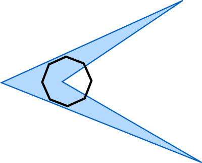
Figure 1: One of a family of $n$ contractible hulls such that all sets of $n-1$ hulls have a common intersection, but not all $n$ do.

Rousseeuw [29] expressed the hope for an alternate proof of Conjecture 1 analogous to that of Lemma 6, based on some formulation of Helly’s theorem for contractible hulls (sets of hyperplanes having nonzero regression depth for some point set). The natural formulation is that, if every sufficiently large subset of a family of contractible hulls has nonempty intersection, then the whole family has nonempty intersection. However, despite some formal similarities between similarly defined shapes and convex polygons [12], there can be no such result, as we now show.

We use the projective dual formulation, in which the contractible hull of an arrangement of lines consists of those points not interior to an infinite cell of the arrangement. Figure 1 shows how, for a regular $n$-gon, one can find a set of four lines such that their contractible hull (the set of points that cannot reach infinity, consisting of a nonconvex quadrilateral together with the points on the lines themselves) contains all but one $n$-gon vertex, does not contain the $n$-gon center, and has its two outer lines perpendicular to the two $n$-gon sides adjacent to the missed vertex. Thus, the hull is completely disjoint from a wedge defined by two rays emanating from the $n$-gon center, parallel to the hull’s two outer lines. If we form $n$ of these hulls, one per $n$-gon vertex, the union of the corresponding wedges is the entire plane; therefore the intersection of the $n$ contractible hulls is empty. However, any subset of $n-1$ hulls do have a common intersection, including at least the $n$-gon vertex missed by the one hull not in the subset.

However, Rousseeuw (personal communication) noted that Theorem 1 does imply some sort of special case of a Helly theorem: the contractible hulls of all $(nd/(d+1))$-tuples of sites have a common intersection. It remains unclear whether this can be formalized as a more general Helly theorem for families of contractible hulls.

6 Analogues of Tverberg’s Theorem

A Tverberg partition of a set of point sites is a partition of the sites into subsets, the convex hulls of which all have a common intersection. (To extend this definition to the projective plane, we define the convex hull of a point at infinity to be the whole plane.) The Tverberg depth of a point $x$ is the maximum cardinality of any Tverberg partition for which the common intersection contains $x$. Note that the Tverberg depth is a lower bound on the location depth. Tverberg’s theorem [36, 37] is that there always exists a point with Tverberg depth $\lceil n/(d+1)\rceil$ (a Tverberg point); this result generalizes both the existence of center points (since any Tverberg point must be a center point) and Radon’s theorem [27] that any $d+2$ points have a Tverberg partition into two subsets.

Similarly, define a contractible partition of a set of point sites to be a partition of the sites into subsets, the contractible hulls of which all have a common intersection, and define the contractible partition number of the set to be the maximum number of subsets in any partition. Conjecture 2 states that the contractible partition number is always at least $\lceil n/(d+1)\rceil$. Since a hyperplane $H$ is in the contractible hull of a set of points if and only if a projective transformation taking $H$ to infinity takes $\hat{\infty}$ to a point in the convex hull of the transformed set, the contractible partition number is the maximum Tverberg depth of the image of $\hat{\infty}$ under any projective transformation. Thus the conjecture would be proven if we could find a projective transformation taking $\hat{\infty}$ to a Tverberg point.

Unfortunately we have not been able to extend our previous proof to this case. We do not know of an appropriate generalization of Tverberg points to continuous measures, and in any case Tverberg points are not very well behaved: the set of Tverberg points need not be connected, if it is connected it need not be simply connected, and in dimensions higher than two its convex hull need not be the set of all centerpoints [35].

However, we can at least show that the contractible partition number is always at least $n/d(d+1)$, an improvement over the previous bound of Steiger and Wenger [34]:

Lemma 10

Let $c$ have location depth $D$ with respect to a set of $n$ sites. Then $c$ has Tverberg depth at least $\lceil D/d\rceil$.

Proof: As long as $c$ is contained in the convex hull of the sites, greedily choose some simplex with site vertices containing $c$ and remove its sites from the set. This process can continue until all sites in some halfspace $H$ containing $c$ on its boundary have been removed. Initially, $H$ has at least $D$ sites, and each simplex can contain only $d$ points in $H$, so at least $\lceil D/d\rceil$ simplices can be chosen before $H$ is exhausted.

Theorem 2

The contractible partition number is at least $\lceil n/d(d+1)\rceil$.

Proof: Find a hyperplane $H$ of regression depth $\lceil n/(d+1)\rceil$ and a projective transformation taking $H$ to the hyperplane at infinity, and apply the lemma to the image of $\hat{\infty}$ under this transformation.

In two dimensions, the optimal bound $\lceil n/3\rceil$ was shown by Rousseeuw and Hubert [31], and a partition achieving this bound can be found in linear time from their construction [15].

7 Better Tverberg Partitions in Three Dimensions

Our general result above implies that in three dimensions there always exists a partition of the sites into $\lceil n/12\rceil$ subsets the contractible hulls of which have a common intersection. We now improve this bound somewhat to $\lfloor(n+1)/6\rfloor$.

The idea behind our bound is to partition the sites by a plane such that the two subsets, when projected onto a horizontal plane, have equal centerpoints. We will then be able to find a Tverberg partition consisting of $\lfloor(n+1)/6\rfloor$ subsets, each formed by a triangle above the partition plane and a triangle below the partition plane, where the triangles come from an equivalence between center points and Tverberg points in $\Bbb R^{2}$:

Lemma 11 (Birch [1])

Let point $x$ be a center point of a set of $3k$ sites in $\Bbb R^{2}$. Then $x$ is also a Tverberg point for this set of sites.

The proof of Birch’s result is simply to form $k$ triangles by connecting every $k$th point in the sequence of sites sorted by their angles around $x$. We need the following strengthening of the lemma:

Lemma 12

Let point $x$ have location depth $k$ in a set of $n>3k$ sites in $\Bbb R^{2}$. Then there is a subset of exactly $3k$ sites, such that $x$ still has location depth $k$ in this subset.

Proof: Since $n\geq 3k+1$, and $k$ is an integer, $\lfloor(n-k-1)/2\rfloor\geq k$. Let $H$ be a closed halfspace with $x$ on its boundary, containing exactly $k$ sites. Sort the sites outside $H$ according to their angles with $x$, and let $y$ be the median site in this sorted order. Then the two closed wedges in the complement of $H$, bounded by line $xy$, each contain at least $\lfloor(n-k-1)/2\rfloor\geq k$ sites, not counting $y$. If we remove $y$ from the set of sites, then the number of sites in any halfspace not containing $y$ does not change, and any halfspace containing $y$ contains one of these two wedges. Therefore, the location depth of $x$ remains equal to $k$ and the result follows by induction on $n$.

Corollary 2

Let point $x$ have location depth $k$ in $n$ point sites in $\Bbb R^{2}$. Then $x$ has Tverberg depth at least $\mathop{\rm min}\{k,\lfloor n/3\rfloor\}$.

Given any oriented plane $P$ in $\Bbb R^{3}$, define $L(P)$ to be the closed halfspace to the left of $P$ (according to the orientation of $P$) and $R(P)$ to be the closed halfspace to the right. Let $\pi:\Bbb R^{3}\mapsto\Bbb R^{2}$ be a vertical projection from $\Bbb R^{3}$ to $\Bbb R^{2}$: that is, $\pi(x,y,z)=(x,y)$. Note that $\pi$ also acts as a continuous function from smooth measures in $\Bbb R^{3}$ to smooth measures in $\Bbb R^{2}$, according to the formula $\pi(m)(S)=m(\pi^{-1}(S))$. If $S$ is any measurable set in $\Bbb R^{3}$, and $m$ is any measure on $\Bbb R^{3}$, let $m\cap S$ denote the measure defined by the formula $(m\cap S)(T)=m(S\cap T)$.

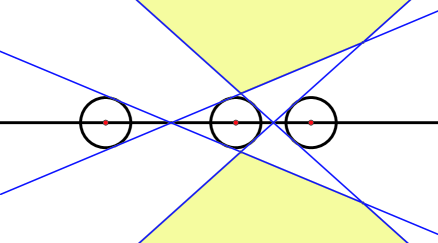
Figure 2: The $\delta$-neighborhood of a line through $\geq 2$ sites.

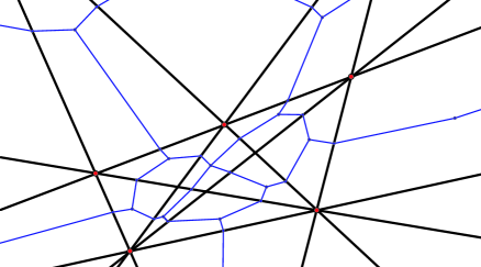
Figure 3: Arrangement of lines determined by pairs of sites, and subdivision of arrangement cells into quadrilaterals.

Given a set of point sites in $\Bbb R^{2}$, define points $c$ and $c^{\prime}$ to be combinatorially equivalent if there is no line determined by two sites that has $c$ on one side and $c^{\prime}$ on the other. Define the $\delta$-neighborhood of a line $L$ through two or more sites to be the set of lines determined by pairs of points within distance $\delta$ of two distinct sites on $L$. The lines of the $\delta$-neighborhood all lie within a region bounded by two convex polygons, with sides formed by lines tangent to radius-$\delta$ circles around the sites on $L$ (Figure 2). We say that a line $L$ determined by two sites $p$ and $q$ is $\delta$-near $c$ if there is a line $L^{\prime}$ through $c$ in the $\delta$-neighborhood of $L$. For any $c$ and $L$ not incident to $c$, $L$ is not $\delta$-near $c$ for all sufficiently small values of $\delta$.

Lemma 13

For any finite set of sites in any bounded region of $\Bbb R^{2}$, there exists a $\delta$ such that, for any point $c$ in the bounded region, we can find a combinatorially equivalent point $c^{\prime}$, having the property that any line through two sites that is $\delta$-near to $c$ passes through $c^{\prime}$.

Proof: We first describe how to map $c$ to $c^{\prime}$; we will then show that there exists an appropriate $\delta$ for this map. Form the arrangement of all lines through two or more sites, find a point $p_{i}$ interior to each cell $C_{i}$ of the arrangement (other than infinite cells with only one vertex), and divide $C_{i}$ into small quadrilaterals by drawing line segments from $p_{i}$ to the midpoints of the finite-length edges of $C_{i}$ (Figure 3). Within infinite cells of the arrangement, we also add a ray from $p_{i}$ to infinity, not parallel to either side of $C_{i}$. Our choice of $c^{\prime}$ is determined by this subdivision: each point $c$ interior to a quadrilateral is mapped to the unique arrangement vertex $c^{\prime}$ contained in that quadrilateral. We can use an arbitrary tie-breaking rule to assign points on the boundaries of quadrilaterals to the arrangement vertex for any incident quadrilateral.

Now approximate the given bounded region by a square that contains it. For any line $L$ determined by two sites, there exists a $\delta_{L}$ such that $L$ is not $\delta_{L}$-near any of the points $p_{i}$, arrangement edge midpoints, arrangement vertices not incident to $L$, or points where the square crosses one of the edges of the subdivision. Each point $c$ in the bounded region that is not mapped to $L$ is contained in the convex hull of some set of these points, all on the same side of $L$. The complement of a $\delta$-neighborhood on one side of $L$ is convex. Therefore, $L$ will not be $\delta_{L}$-near any point $c$ mapped to a $c^{\prime}$ not on $L$. We simply choose $\delta$ to be the minimum of the values $\delta_{L}$.

Theorem 3

The contractible partition number in $\Bbb R^{3}$ is at least $\lfloor\lceil n/2\rceil/3\rfloor=\lfloor(n+1)/6\rfloor$.

Proof: Let $\delta$ be small enough that we can apply Lemma 4 to the sites and Lemma 13 to the vertical projection of the sites (with the bounded region of Lemma 13 being the points within distance $\delta$ of the convex hull of the sites). Let $\epsilon<1/18$, and find a smooth nowhere zero measure $m$ on $\Bbb R^{3}$ such that the total measure is $n-2\epsilon$, the measure within the radius-$\delta$ ball around any site is at most one, and the total measure outside all such balls is at most $\epsilon$. Let $\mu$ be a nowhere zero smooth measure on $\Bbb R^{2}$ with total measure $\epsilon$.

For each unit vector $u$ in $\Bbb R^{3}$, let $P(u)$ denote the oriented plane normal to $u$ for which $m(L(P))=m(R(P))$. Note that $P(u)$ is unique due to the assumption that $m$ is nowhere zero. Let $f(u)$ denote the vector difference between two points in $\Bbb R^{2}$: the $\epsilon$-trimmed means of $\pi(m\cap L(P))+\mu$ and $\pi(m\cap R(P))+\mu$. That is, if these two $\epsilon$-trimmed means have Cartesian coordinates $(x_{L},y_{L})$ and $(x_{R},y_{R})$ then let $f(u)$ be the vector $(x_{L}-x_{R},y_{L}-y_{R})$. Then $f$ is a continuous antipodal function, so by the Borsuk-Ulam Theorem [2] it has a zero $u$, where the two $\epsilon$-trimmed means coincide at a common point $c$.

Use Lemma 4 to find a plane $P^{\prime}$ passing through all sites within distance $\delta$ of $P(u)$; then $L(P^{\prime})$ and $R(P^{\prime})$ each contain at least $\lceil n/2-\epsilon\rceil=\lceil n/2\rceil$ sites. Use Lemma 13 to find a point $c^{\prime}\in\Bbb R^{2}$ on any line $\delta$-near $c$.

Then $c^{\prime}$ must have location depth at least $\lceil n/6\rceil$ with respect to each of the two planar sets formed by vertically projecting $L(P^{\prime})$ and $R(P^{\prime})$. For, let $h^{\prime}$ be a closed halfplane with $c^{\prime}$ on its boundary, containing as few points as possible from $L(P^{\prime})$ or $R(P^{\prime})$; let $k=\mathop{\rm min}\{|h^{\prime}\cap L(P^{\prime})|,|h^{\prime}\cap R(P^{\prime})|\}$. Since $c^{\prime}$ is not $\delta$-near any line it is not incident to, we can rotate $h^{\prime}$ if necessary to a combinatorially equivalent halfplane such that the boundary of $h^{\prime}$ does not pass within distance $\delta$ of any nonincident point. Next, translate the halfplane so that its boundary moves from $c^{\prime}$ towards $c$ without coming within distance $\delta$ of any site outside $h^{\prime}$. If the halfplane gets stuck by becoming tangent to a radius-$\delta$ circle around a site, rotate it towards $c$ while keeping it tangent to that circle. This rotation process can not become stuck by hitting another such circle, because the two corresponding sites would determine a line that either separates $c$ from $c^{\prime}$ or is $\delta$-near to $c$, neither of which can happen by Lemma 13. So the result of this process must be a halfplane $h$, with boundary incident to $c$, that is at distance at least $\delta$ from any site not in $h^{\prime}$. Therefore, $h$ intersects the radius-$\delta$ circles around at most $k$ sites of $L(P^{\prime})$ or $R(P^{\prime})$, so $\mathop{\rm min}\{(\pi(m\cap L(P))+\mu)(h),(\pi(m\cap L(P))+\mu)(h)\}\leq k+2\epsilon$. But, since $c$ is an $\epsilon$-trimmed mean, $\mathop{\rm min}\{(m\cap L(P)+\mu)(h),(m\cap L(P)+\mu)(h)\}\geq n/6-\epsilon$. Therefore, $k\geq n/6-3\epsilon$, and, since $\epsilon<1/18$ and $k$ is an integer, $k\geq\lceil n/6\rceil$.

By Corollary 2, we can find a set $TL$ of $\lfloor\lceil n/2\rceil/3\rfloor$ triangles having as vertices sites in $L(P^{\prime})$, such that the projection of each triangle contains $c^{\prime}$, and a corresponding set $TR$ of $\lfloor\lceil n/2\rceil/3\rfloor$ triangles with vertices in $R(P^{\prime})$.

We now use these triangles to form contractible hulls containing $P^{\prime}$. Whenever some triangle has a vertex $v$ on plane $P^{\prime}$, we form the contractible hull of $v$ itself; this consists of all planes passing through $v$ and in particular $P^{\prime}$. When we do this, we remove from $TL$ and $TR$ any triangle using $v$ as a vertex. Once all remaining vertices are disjoint from $P^{\prime}$, all the triangles are disjoint from each other. We then arbitrarily choose pairs of triangles, one from $TL$ and one from $TL$, until we run out of triangles in one of the two sets. Each of the pairs gives a six-site set with contractible hull containing $P^{\prime}$, because the triangle above $P^{\prime}$ and the triangle below $P^{\prime}$ project to sets with intersecting convex hulls: specifically, their intersection contains the point $c^{\prime}$.

8 NP-hardness

We now briefly discuss the computational complexity of testing the regression depth or contractible partition number for a given plane. Clearly, when the dimension is a fixed constant, the regression depth can be tested in time $O(n^{d-1}+n\mathop{\rm log}n)$: there are $O(n^{d-1})$ combinatorially distinct vertical hyperplanes, the set of these vertical hyperplanes can be constructed by forming a arrangement in a space dual to the $(d-1)$-dimensional projection of the points, and the number of points in each double wedge defined by a vertical hyperplane and the input hyperplane can be found in constant time by walking from cell to cell in this dual arrangement. Standard $\epsilon$-cutting methods [23] can be used to design an algorithm to approximate the regression depth within a $(1+\epsilon)$ factor, in linear time for any fixed values of $\epsilon$ and the dimension.

When the dimension is not a fixed contant, testing whether the location depth of a point is at least some fixed bound is coNP-complete [17]. Teng [35] showed that the special case of testing whether a point is a center point is still coNP-complete.

Theorem 4

Testing whether a hyperplane has regression depth at least $n/(d+1)$ is coNP-complete.

Proof: First, to show that a hyperplane does not have high regression depth, we need merely exhibit a double wedge bounded by it and a vertical hyperplane that contains few points. Therefore, the problem of testing regression depth is in coNP.

If one could compute regression depth, one could use this to compute the location depth of a point $x$ by finding a projective transformation taking $x$ to $\hat{\infty}$ and testing the regression depth of the image of the hyperplane at infinity. This transformation is a reduction from testing center points to testing regression depth; therefore testing regression depth is coNP-complete.

Therefore, also, computing the regression depth of a hyperplane is NP-hard, since one could test regression depth by comparing the computed depth to the value $n/(d+1)$. However, these results do not rule out the possibility of an efficient algorithm for finding a deep hyperplane.

Teng [35] also showed that the problem of testing whether the Tverberg depth of a point is at least some fixed bound, or of testing whether the point is a Tverberg point, is NP-complete. Using the same transformational ideas as before, this leads immediately to the following result:

Theorem 5

Testing whether a hyperplane has contractible partition number at least $n/(d+1)$ is NP-complete.

The computational complexity of computing a deep hyperplane or a hyperplane with high contractible partition number remains open.

Acknowledgements

Work of Amenta, Eppstein, and Teng was performed in part while visiting the Xerox Palo Alto Research Center. David Eppstein’s work was supported in part by NSF grant CCR-9258355 and by matching funds from Xerox Corp. Shang-Hua Teng’s work was supported in part by an Alfred P. Sloan Fellowship.

The authors would like to acknowledge helpful conversations with Zbigniew Fiedorow, Harald Hanche-Olsen, Dan Hirschberg, Mia Hubert, Peter Rousseeuw, Jack Snoeyink, Rafe Wenger, and Frances Yao.

References

- [1] B. J. Birch. On points in a plane. Proc. Cambridge Phil. Soc. 55(4):289–293, 1959.
- [2] K. Borsuk. Drei Sätze über die -dimensionale euklidische Sphäre. Fund. Math. 20:177–190, 1933.
- [3] H. Brönnimann and B. Chazelle. Optimal slope selection via cuttings. Computational Geometry: Theory & Applications 10(1):23–29, April 1998.
- [4] L. E. J. Brouwer. Über eineindeutiger stetige Transformationen von Flächen in sich. Math. Annalen 69:176–180, 1910.
- [5] L. E. J. Brouwer. Über Abbildung von Mannigfaltigkeiten. Math. Annalen 71:97–115, 1912.
- [6] K. L. Clarkson, D. Eppstein, G. L. Miller, C. Sturtivant, and S.-H. Teng. Approximating center points with iterated Radon points. Int. J. Computational Geometry & Applications 6(3):357–377, September 1996.
- [7] R. Cole, J. S. Salowe, W. Steiger, and E. Szemerédi. An optimal-time algorithm for slope selection. SIAM J. Computing 18(4):792–810, August 1989.
- [8] H. S. M. Coxeter. Projective Geometry. Springer Verlag, 2nd edition, 1987.
- [9] L. Danzer, B. Grünbaum, and V. Klee. Helly’s theorem and its relatives. Proc. Symposia in Pure Mathematics, vol. 7, pp. 101–180. AMS, 1963.
- [10] M. B. Dillencourt, D. M. Mount, and N. S. Netanyahu. A randomized algorithm for slope selection. Int. J. Computational Geometry & Applications 2(1):1–27, March 1992.
- [11] H. Edelsbrunner and D. L. Souvaine. Computing least median of squares regression lines and guided topological sweep. J. Amer. Statistical Assoc. 85(409):115–119, March 1990.
- [12] D. Eu, E. Guévremont, and G. T. Toussaint. On envelopes of arrangements of lines. J. Algorithms 21(1):111–148, July 1996.
- [13] F. R. Hampel, E. M. Ronchetti, P. J. Rousseeuw, and W. A. Stahel. Robust Statistics: the Approach Based on Influence Functions. Series in Probability and Mathematical Statistics. Wiley Interscience, 1986.
- [14] E. Helly. Über Mengen konvexer Körper mit gemeinschaftlichen Punkten. Jber. Deutsch. Math.-Verein. 32:175–176, 1923.
- [15] M. Hubert and P. J. Rousseeuw. The catline for deep regression. J. Multivariate Analysis 66:270–296, 1998, http://win-www.uia.ac.be/u/statis/publicat/catline_abstr.html.
- [16] S. Jadhav and A. Mukhopadhyay. Computing a centerpoint of a finite planar set of points in linear time. Discrete & Computational Geometry 12(3):291–312, October 1994.
- [17] D. S. Johnson and F. P. Preparata. The densest hemisphere problem. Theoretical Computer Science 6:93–107, 1978.
- [18] M. J. Katz and M. Sharir. Optimal slope selection via expanders. Information Processing Lett. 47(3):115–122, September 1993.
- [19] M. van Kreveld, J. S. B. Mitchell, P. J. Rousseeuw, M. Sharir, J. Snoeyink, and B. Speckmann. Efficient algorithms for maximum regression depth. Proc. 15th Symp. Computational Geometry, pp. 31–40. ACM, June 1999.
- [20] S. Langerman and W. Steiger. An algorithm for the hyperplane median in . Manuscript, 1999.
- [21] J. Matoušek. Randomized optimal algorithm for slope selection. Information Processing Lett. 39(4):183–187, August 1991.
- [22] D. M. Mount, N. S. Netanyahu, K. Romanik, R. Silverman, and A. Y. Wu. A practical approximation algorithm for the LMS line estimator. Proc. 8th Symp. Discrete Algorithms, pp. 473–482. ACM and SIAM, 1997.
- [23] K. Mulmuley and O. Schwarzkopf. Randomized algorithms. Handbook of Discrete and Computational Geometry, chapter 34, pp. 633–652. CRC Press, 1997.
- [24] N. Naor and M. Sharir. Computing a point in the center of a point set in three dimensions. Proc. 2nd Canad. Conf. Computational Geometry, pp. 10–13. Univ. of Ottawa, Dept. of Computer Science, August 1990.
- [25] J. C. Oxtoby. Measure and Category. Graduate Texts in Mathematics 2. Springer Verlag, 2nd edition, 1980.
- [26] R. Rado. A theorem on general measure. J. London Math. Soc. 21:292, 1946.
- [27] J. Radon. Mengen konvexer Körper, die einen gemeinsamen Punkt Enthalten. Math. Annalen 83:113–115, 1921.
- [28] P. J. Rousseeuw. Least median of squares regression. J. Amer. Statistical Assoc. 79:871–880, 1984.
- [29] P. J. Rousseeuw. Computational geometry issues of statistical depth. Invited talk at 14th ACM Symp. Computational Geometry, Minneapolis, 7 June 1998.
- [30] P. J. Rousseeuw and M. Hubert. Depth in an arrangement of hyperplanes. To appear in Discrete & Computational Geometry, http://win-www.uia.ac.be/u/statis/publicat/arrang_abstr.html.
- [31] P. J. Rousseeuw and M. Hubert. Regression depth. J. Amer. Statistical Assoc. 94, June 1999, http://win-www.uia.ac.be/u/statis/publicat/rdepth_abstr.html.
- [32] P. J. Rousseeuw and A. M. Leroy. Robust Regression and Outlier Detection. Series in Applied Probability and Statistics. Wiley Interscience, 1987.
- [33] P. J. Rousseeuw and A. Struyf. Computing location depth and regression depth in higher dimensions. Statistics and Computing 8(3):193–203, August 1998, http://win-www.uia.ac.be/u/statis/publicat/compdepth_abstr.html.
- [34] W. Steiger and R. Wenger. Hyperplane depth and nested simplices. Proc. 10th Canad. Conf. Computational Geometry. McGill Univ., 1998, http://cgm.cs.mcgill.ca/cccg98/proceedings/cccg98-steiger-hyperplane.ps%.
- [35] S.-H. Teng. Points, Spheres, and Separators: a Unified Geometric Approach to Graph Partitioning. Ph.D. thesis, Carnegie-Mellon Univ., School of Computer Science, August 1991.
- [36] H. Tverberg. A generalization of Radon’s theorem. J. London Math. Soc. 41:123–128, 1966.
- [37] H. Tverberg. A generalization of Radon’s theorem II. Bull. Austral. Math. Soc. 24(3):321–325, 1981.