Separation-Sensitive Collision Detection for Convex Objects

Abstract

We develop a class of new kinetic data structures for collision detection between moving convex polytopes; the performance of these structures is sensitive to the separation of the polytopes during their motion. For two convex polygons in the plane, let $D$ be the maximum diameter of the polygons, and let $s$ be the minimum distance between them during their motion. Our separation certificate changes $O(\log(D/s))$ times when the relative motion of the two polygons is a translation along a straight line or convex curve, $O(\sqrt{D/s})$ for translation along an algebraic trajectory, and $O(D/s)$ for algebraic rigid motion (translation and rotation). Each certificate update is performed in $O(\log(D/s))$ time. Variants of these data structures are also shown that exhibit hysteresis—after a separation certificate fails, the new certificate cannot fail again until the objects have moved by some constant fraction of their current separation. We can then bound the number of events by the combinatorial size of a certain cover of the motion path by balls.

1 Introduction

Collision detection is an algorithmic problem arising in all areas of computer science dealing with the simulation of physical objects in motion. Examples include motion planning in robotics, virtual reality animations, computer-aided design and manufacturing, and computer games. Often the problem is broken up into two parts, the so-called broad phase, in which we identify the pairs of objects we need to consider for possible collision, and the narrow phase in which we track the occurrence of collisions between a specific pair of objects [Hub]. (In the spatial database literature, these are also called the filtering and refinement phases, respectively [Ore].) For the broad phase, almost all authors use some kind of simple bounding volumes for the objects themselves, or for portions of their trajectories in space or space-time, so as to quickly eliminate from consideration pairs of objects that cannot possibly collide. The narrow phase is more specialized, according to the types of objects being considered.

The simplest objects to consider are convex polytopes (polygons in the plane, or polyhedra in 3-space), and this case has been extensively considered in the literature [LC, Mir, MC, GJK, CW]. More complex objects are then broken up into convex pieces, which are tested pairwise. Algorithmically, the convex polytope intersection problem is a special case of linear programming; in two and three dimensions even more efficient techniques have been developed in computational geometry, that can be applied after a suitable preprocessing of the two polytopes [DHKS, 7]. The methods, however, that have proven to work best in practice exploit the temporal coherence of the motion to avoid doing an ab initio intersection test at each time step. Not surprisingly, the collision detection problem is closely related to the distance computation problem. Since the distance between two continuously moving polytopes also changes continuously, many well-known collision detection algorithms, such as those of Lin and Canny [Lin, LC], Mirtich [Mir, MirV, MC], and Gilbert et al. [GJK] (see also [Cam]), are based upon tracking the closest pair of features of the polytopes during their motion (which, of course, implies knowledge of the distance between the polytopes). The efficiency of these algorithms is based on the fact that, in a small time step, the closest pair of features will not change, or will change to some nearby features on the polytopes.

Though it is hard to imagine how one can do better than tracking the closest pair of feature when the polytopes are in close proximity, such tracking seems to be unnecessarily complicated when the polytopes start moving further from each other. Indeed most of the above authors suggest performing first a simple bounding volume (box or sphere) test on the two polytopes, and only if that fails entering the closest feature pair tracking mode. In this paper we consider a number of general techniques that allow us to perform collision detection between two moving convex polytopes in a way that is sensitive to the separation between the polytopes. In order to properly quantify the separation-sensitivity of our methods, we view the collision detection problem in the context of kinetic data structures (or KDSs for short), introduced in [2, 12].

In the kinetic setting we assume that the instantaneous motion laws for our polytopes are known, though they can be changed at will by appropriately notifying the KDS. Our sampling of time is not fixed, but is determined by the failure of certain conditions, called certificates. In our case these are separation certificates, which prove that the two polytopes do not intersect. The failure of a separation certificate need not mean that a collision has occurred; it can simply mean that that certificate has to be replaced by one or more others, still proving the non-intersection of the polytopes. A good KDS is compact if it requires little space, responsive if it can be updated quickly after a certificate failure, local if it adjusts easily to changes in the motion plans of the objects, and efficient if the total number of events is small. Our kinetic collision-detection data structures have all these properties; they maintain only a small constant number of certificates, and the cost for processing a certificate failure or a motion plan update is at most polylogarithmic (in the combinatorial size of the polytopes).

A number of the papers referenced above make the claim that their algorithms are efficient because “if the sampling interval is small enough, then the cost of updating the closest pair of features is $O(1)$.” This is a difficult statement to attach a fully rigorous meaning to—exactly how small the time step must be to guarantee this condition depends a great deal on both the polytopes and the speed and complexity of their motion. In the kinetic setting we can give the notion of efficiency a more satisfactory theoretical definition, by focusing on the maximum number of certificate failures we may have to process for polytopes and motions of a certain complexity, rather than on the adequacy of any absolute unit of time.

The key contribution of this paper is to develop a class of new kinetic data structures for collision detection between convex polytopes, where the efficiency of the structure can be analyzed in terms of natural attributes of the motion. Given two moving convex polygons in the plane, let $\mu=\min\{n,\sqrt{D/\sigma}\}$, where $n$ is the combinatorial complexity of the polygons, $D$ is their maximum diameter, and $\sigma$ is their minimum separation during the entire motion. In Section 5 we develop a KDS where the number of events (certificate failures) is $O(\log\mu)$ when the relative motion of the two polygons is translation along a convex trajectory (for example, a straight line), $O(\mu)$ for translation along a algebraic trajectory, and $O(\mu^{2})$ for algebraic rigid motion (translation and rotation). Thus we see how the nature of the motion, as well as the proximity of the two polygons, affect the complexity of the collision detection problem.

In contrast to this, the closest pair of features of two polygons can change $\Omega(n^{2})$ times under an algebraic rigid motion, no matter what their separation is. For ‘intermediate separation’ situations, when the bounding boxes of two objects intersect, but their distance is still $\Omega(D)$, our methods will perform much better than other extant methods for collision detection. The performance of our methods interpolates smoothly those of the bounding box and closest pair of features techniques mentioned above, as the separation varies. In this intermediate distance range our methods are also directly useful for non-convex objects, as such objects can be bounded by their convex hulls.

We attain these distance-sensitive bounds by constructing certain novel outer approximating hierarchies for our polytopes, whose structure is of independent interest. These hierarchies provide a series of combinatorially simpler and simpler shells, as we move away from the polytope. For two polytopes in proximity the hierarchies locally refine so as to provide a separation certificate.

Hidden in the above ‘$O$’ bounds are factors depending on the algebraic degree of the motion. Again, when the polytopes are in close proximity, it is clear why a ‘wiggly’ motion should be more costly than a smooth one. But why should it be so when they are further away? This has motivated us to develop structures that exhibit hysteresis—where, after a certificate failure has occurred, no other certificate failure can happen until the objects have moved by some constant fraction of their current separation. Using these structures, we are able to bound the number of events by the combinatorial size of a certain cover of the motion path by balls (Section 6), somewhat reminiscent of [21].

We believe that the KDSs shown here are of theoretical and practical interest. A basic tool for all our structures are certain outer approximation hierarchies for convex polytopes and their Minkowski sums—a topic which we believe to be of independent interest (Section 3). The distance- and motion-sensitive bounds we give are novel and, to our knowledge, the first such to be ever presented.

It was surprising to us that even for the simple setting of two moving convex polygons, there is much that is novel and interesting to say; in fact, many challenging open questions remain. Though our exposition is focussed on the two-dimensional case, we do not anticipate significant obstacles in extending our results to three dimensions; we briefly describe some preliminary results in Section 7. We expect that our kinetic structures will lead to improved practical algorithms for convex shapes, and we have already started an implementation of our algorithms. In a companion paper [3], we discuss a different set of kinetic collision techniques applicable to non-convex shapes.

2 Models of motion

In our model, each object is a closed rigid convex polygon, whose motion is described by a moving orthogonal reference frame: a point $o(t)$ and two orthogonal unit vectors $x(t),y(t)$, whose coordinates are continuous algebraic functions of $t$. (Such moving frames do exist, and are flexible enough to approximate any motion to any order and accuracy, for a limited time. Note however that an algebraic rotation is necessarily of non-uniform angular velocity, and can cover only $O(d)$ full turns, where $d$ is the degree of the entries.) Each vertex of the object is assumed to have constant algebraic coordinates $(X,Y)$ relative to the frame $(o,x,y)$; so that its position at time $t$ is $o(t)+Xx(t)+Yy(t)$, also an algebraic function of $t$.

As we shall see, the certificates used in each of our KDSs have the general form $F(t)=G(p_{1}(t),\dots,p_{n}(t))$. Here $p_{1}(t),\dots,p_{m}(t)$ are the positions of $m$ vertices ($m$ will be a small constant), possibly on different objects; and $G$ is some algebraic function. Then $F$ itself is an algebraic function, which means we can compute the next time $t$ when $F(t)=0$, exactly, and compare any two times, at finite cost, within an appropriate arithmetic model. Moreover, the number of zeros of $F$ in any finite interval is bounded by its algebraic degree, which is the degree of $G$ times the maximum algebraic degree $d$ among the motion coordinates. So, for, example, the same vertex triplet cannot become collinear more than $2d$ times.

In conclusion, if the complexity (algebraic degree and coefficient size) of the motions is bounded, each certificate can fail at most $O(1)$ times during a single motion, and the cost of computing and comparing the failure times is also $O(1)$. We will use these last two facts, and only these two facts, throughout our analyses. Our results do not require any other combinatorial properties of algebraic motion—for example, that an algebraic path can be decomposed into a constant number of convex sub-paths, as in the companion paper [3]—and therefore apply to a wider range of pseudo-algebraic motions [2, 12].

3 Polygon Approximation Hierarchies

Our collision detection algorithms are based on outer approximation hierarchies for the convex polygons involved, or for their Minkowski sum. All these hierarchies tile the space exterior to the polygon so as to simplify the combinatorial structure of the polygon as one goes away from the polygon. A well-known example of such a hierarchy in computational geometry is the Dobkin-Kirkpatrick hierarchy [7]. This hierarchy is not by itself adequate for our purposes, however, as it is not sensitive to the distance away from the polygon; any approximation in the hierarchy can have vertices arbitrarily far from the original polygon. We will retain a key property of this hierarchy, namely the fact that that each ‘coarsening step’ is performed by removing an existing edge of the current approximation and extending outwards its two neighboring edges till they meet. However, in order to guarantee that we get the distance-sensitivity that we require, we will enrich the set of ‘available edges’ by introducing an additional set of degenerate edges around the polygon, initially all of zero length. In general, the number of these degenerate edges will be proportional to the number of original edges in the polygon.

Though one normally thinks of these approximating hierarchies as being constructed from the boundary of the polygon towards the outside, it is actually advantageous to visualize this process in reverse. Let $P$ be our convex polygon of $n$ edges. We start from the outermost approximation $P_{0}$, which for our purposes is always a (not necessarily axis-aligned) bounding rectangle of $P$. The space between $P$ and $P_{0}$ comprises up to four non-convex polygons, each consisting of a concave chain and two additional edges. Following Hershberger and Suri [HS], we call these polygons boomerangs. The last coarsening step, if undone, corresponds to ‘cutting off a corner’ of $P_{0}$ through the reintroduction of another (possibly degenerate) edge of $P$. This step splits one of the top-level boomerangs into a triangle and two smaller boomerangs. This process of cutting off corners is continued recursively, until all edges of $P$ have been reintroduced. See Figure 1. Structurally, the hierarchy consists of four binary trees, where each internal node corresponds to a triangle and each subtree to a boomerang. In our hierarchies, each of these trees will have depth $O(\log n)$. A variety of outer approximations for $P$ can be defined by removing a subtree of triangles rooted at each of the top-level boomerangs.

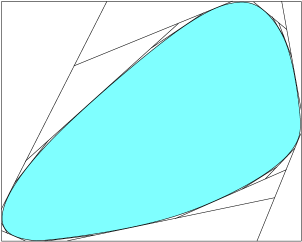
Figure 1: A boomerang hierarchy.

Before we discuss various choices of degenerate edges, let us develop some notation and terminology. The apex of a boomerang is the unique vertex not on the boomerang’s concave chain. The height of a boomerang is the distance from its apex to its concave chain; this is the maximum distance from any point in the boomerang to the chain. The level of either a boomerang or a triangle is its depth from the root in the appropriate binary tree; there are at most $4\cdot 2^{i}$ boomerangs at level $i$. Finally, let $P_{i}$ denote the $i$-th envelope of $P$, defined as the union of $P$ and all level-$i$ boomerangs; $P_{i}$ is itself a convex polygon surrounding $P$.

Let $D$ denote the diameter of $P$. The following lemma implies that the envelopes in any boomerang hierarchy of $P$ are reasonably close to $P$. We omit the easy proof from this abstract.

Lemma 3.1

In any single level of any boomerang hierarchy, there are $O\big{(}\sqrt{D/s}\big{)}$ boomerangs of height at least $s$.

A line $\ell$ that does not intersect $P$ can intersect at most one of the four top-level boomerangs in any boomerang hierarchy of $P$. Moreover, if $\ell$ intersects a boomerang, then it intersects at most one of its two sub-boomerangs. In fact, these two observations hold for any convex curve (bending away from $P$). These simple observations establish the following useful lemma.

Lemma 3.2

Any convex curve disjoint from $P$ intersects at most one triangle in each level of any boomerang hierarchy of $P$.

We observe that the triangles in a boomerang hierarchy for $P$ tile the space between $P_{0}$ and $P$. (It is not hard to extend this tiling to be the complement of $P$ in the plane by allowing a few infinite triangles. This is almost identical to the construction of a binary space partition tree [9].) For a point $x$ outside $P$, the triangle in this tiling that contains $x$ provides us with useful information about the position of $x$ with respect to $P$: the base of the triangle is a side of $P$ separating $x$ from $P$, while the height of the associated boomerang is an upper bound on the distance from $x$ to $P$.

3.1 The Compass Hierarchy

For the compass hierarchy we introduce $O(n)$ zero-length edges into $P$, whose outer normals form a regular recursive lattice on the unit circle, in the standard compass directions (E, N, W, S, NE, NW, SW, SE, etc.). In the top $\lceil\log_{2}n\rceil$ levels of the compass hierarchy, each boomerang is subdivided into two smaller boomerangs and an isosceles triangle. In the remaining levels, if any, each boomerang is subdivided by a line through its median edge, as in a standard Dobkin-Kirkpatrick hierarchy. The resulting hierarchy has at most $2\lceil\log_{2}n\rceil$ levels.

Lemma 3.3

(a) A level-$i$ boomerang in the compass hierarchy of $P$ has height $O(D/2^{i})$.

(b) The compass hierarchy of $P$ contains $O\big{(}\sqrt{D/s}\,\log(D/s)\big{)}$ boomerangs with height at least $s$.

(c) Any convex curve at distance $s$ from $P$ intersects $O(\log(D/s))$ triangles in the compass hierarchy of $P$.

(d) If two polygons $P$ and $Q$ are distance $s$ apart, their compass hierarchies contain disjoint approximations $\widetilde{P}$ and $\widetilde{Q}$, each with $O(\log(D/s))$ edges.

Klosowski et al. [15] define the “$k$-DOP” or discrete orientation polytope of an object to be the bounding polytope whose facets are normal to a fixed set of $k$ ‘compass’ directions. Klosowski et al. construct a hierarchy of bounding volumes for any object by computing the object’s $k$-DOP, decomposing the object into a constant number of pieces, and recursively constructing a hierarchy for each piece, using the same value of $k$ at all levels. (See [BCGMT, GLM, ZF] for similar bounding volume hierarchies.) In contrast, the compass hierarchy consists of a nested sequence of $k$-DOPs with $k=4,8,16,\dots$, all for the same object.

3.2 The Dudley Hierarchy

Our second boomerang hierarchy is based on a result of Dudley [Dud] on approximating convex bodies in arbitrary dimensions by polytopes with few facets; hence, we call it the Dudley hierarchy. Let $S$ be a set of $n$ regularly spaced points on a circle of radius $2D$, centered inside $P$. For each point $x\in S$, let $n(x)$ be its nearest neighbor on $P$. If $n(x)$ is a vertex of $P$, we introduce a zero-length edge at $n(x)$ whose outer normal vector is $n(x)-x$. Otherwise, we introduce a new degenerate vertex at $n(x)$ whose external angle is zero. See Figure 2. We then create a boomerang hierarchy, starting with the bounding box $P_{0}$, by recursively subdividing each boomerang by a line through its median (possibly degenerate) edge (and possibly through other collinear edges). The resulting Dudley hierarchy has depth at most $\lceil\log_{2}(2n)\rceil$.

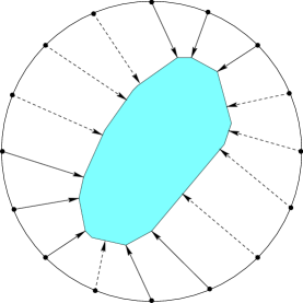
Figure 2: The Dudley construction. Solid vectors introduce degenerate edges; dashed vectors introduce degenerate vertices.

Lemma 3.4

(a) A level-$i$ boomerang in the Dudley hierarchy of $P$ has height $O(D/4^{i})$ [Dud].

(b) The Dudley hierarchy of $P$ contains $O\big{(}\sqrt{D/s}\big{)}$ boomerangs with height at least $s$.

(c) Any convex curve at distance $s$ from $P$ intersects $O(\log(D/s))$ triangles in the Dudley hierarchy of $P$.

(d) If two polygons $P$ and $Q$ are distance $s$ apart, their Dudley hierarchies contain disjoint approximations $\widetilde{P}$ and $\widetilde{Q}$, each with $O(\log(D/s))$ edges.

4 Mixed Hierarchies

The hierarchies introduced so far are tilings of the free space around a single convex polygon. Since we are interested in systems with two (or more) moving convex polygons, we would like to extend some of these notions to hierarchical tilings of the free part of the configuration space generated by the motion of two polygons. Our general plan is to associate (explicitly or implicitly) a particular separation proof with each tile of such a tiling. As the two polygons move and their configuration crosses out of its current tile, some certificates will fail and a new separation certificate will have to be generated.

Let $P$ and $Q$ be our two moving polygons. If $P$ and $Q$ are only translating with respect to each other, then the configuration space remains two-dimensional. It is well-known that in this case the free space is the complement of the convex polygon $P\oplus(-Q)$, the Minkowski sum of $P$ with the negative of $Q$. Since again our two-dimensional configuration space is the exterior of a convex polygon, then all the hierarchies presented above can be directly used, if we are willing to construct this polygon. Such a direct approach, however, is less attractive when rotation is allowed, as then the configuration space can have quadratic combinatorial complexity. Also, for applications where we have multiple moving polygons (though we do not discuss techniques for this many-body problem in this paper), we want to ‘recycle’ as much as possible pieces of the hierarchies built for each of the polygons, rather than having to build a separate hierarchy for each pair.

We describe below one such hierarchy for tiling the complement of the Minkowski sum of two convex polygons into triangles and parallelograms, which we call the mixed hierarchy. (Without loss of generality, we focus on describing this hierarchy for $P\oplus Q$, as opposed to $P\oplus(-Q)$.) It is motivated by the theory of mixed volumes of convex bodies [23], and it has the advantage that it changes in a very regular way as the polygons rotate. This makes it possible to maintain a non-intersection certificate for two moving convex polygons by separating the motion into a translational part, corresponding to a point moving around in the plane, and a rotational part, corresponding to a deformation of the triangle or parallelogram containing the point. At certain discrete events this tile and a neighboring tile are deleted and replaced by two other tiles covering the same area, much like a Delaunay flip. Thus, we can maintain a separation proof by maintaining one tile, or a small working set of tiles, around the current configuration point.

Given two boomerang hierarchies for $P$ and $Q$, the mixed hierarchy is defined by starting from $P_{0}\oplus Q_{0}$ and then interleaving the ‘corner cutting’ operations leading to $P$ and $Q$. Different mixed hierarchies may be obtained for different interleavings of these corner cutting operations. The main difference from a standard boomerang hierarchy arises because the corner of $P$ or $Q$ being cut next may no longer be a corner at all in the Minkowski sum hierarchy: between two consecutive sides of $P$ we can have many sides of $Q$, and vice versa. To be concrete, say the next cut is to add a side $e$ of $P$, but its neighboring sides in the $P$ hierarchy are now separated by a chain of $Q$ edges in the mixed hierarchy built so far. Note that these neighboring sides must already be present in the mixed hierarchy, as the joint corner cutting sequence is consistent with that for $P$. To insert $e$ into the mixed hierarchy, we fist find the place where $e$ fits, according to slope, in the chain of $Q$-edges that replaced its corner. We partition that $Q$-chain at that point, and then translate the two subchains inwards, as illustrated in Figure 3. The two chains come to rest when they encounter the points where $e$ meets its two neighboring edges in $P$. Thus this process adds to the mixed hierarchy exactly the same triangle that it added in the $P$ hierarchy, as well as several parallelograms based on the edges of the $Q$ chain. After all the corners have been cut, the space between $P_{0}\oplus Q_{0}$ and $P\oplus Q$ is tiled with one copy of each of the original triangles used in the $P$ and $Q$ hierarchies, as well as several ‘mixed’ parallelograms.

Figure 3: Inserting an edge into the mixed hierarchy.

Figure 4 shows a full mixed hierarchy for two small convex polygons. The corner cutting order is indicated by the numbers next to the edges of the polygons.

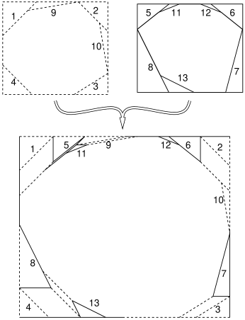
Figure 4: A mixed hierarchy for two convex polygons.

As we mentioned earlier, a nice aspect of the mixed hierarchy is its behavior under polygon rotation. The rotation changes the interleaving of the edges of $P$ and $Q$ around their Minkowski sum. For example, an edge of $P$ can pass in slope ordering one of the edges of the $Q$-chain that it splits. The primary effect of this change on the mixed hierarchy is a simple change, which we call a a page turn, akin to a Delaunay flip: a triangle and a parallelogram exchange positions. Additionally, at some finer level of the hierarchy, one parallelogram may either collapse to a line segment and be destroyed, or a new parallelogram may be created and expand from a line segment. See Figure 5.

Lemma 4.1

If the corner cutting operations for polygons $P$ and $Q$ of size $n$ and $m$, where $m\leq n$, are interleaved according the level of the boomerang destroyed at each step (in the $P$ or $Q$ hierarchy respectively), then the size of the mixed hierarchy is $O((m+n)\log m)$.

Lemma 4.2

If $P$ is stationary and $Q$ makes a single full rotation, then the number of page turns that will happen is $O(mn\log m)$.

Lemma 4.3

Given a cell $c$ of the mixed hierarchy, a point $p\in\partial c$, and some auxiliary structures of linear size for $P$ and $Q$, the neighboring cell of $c$ containing $p$ can be computed in $O(\log n)$ time. The same applies for the cells covering $c$, when cell $c$ is destroyed during a page turn event.

If the boomerang hierarchies of $P$ and $Q$ satisfy distance properties such as those in Section 3, then similar results will hold for the tiles of the mixed hierarchy. For example, if we mix two compass or Dudley hierarchies, we can reduce the time bound in Lemma 4.3 from $O(\log n)$ to $O(\log(D/s))$, where $s$ is the distance from $p$ to $P\oplus Q$.

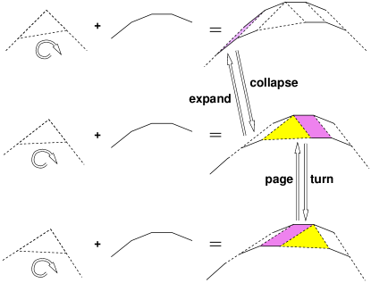
Figure 5: Events in the mixed hierarchy under rotation.

In general, however, the mixed hierarchy does not satisfy the equivalent of Lemma 3.2. Although any line disjoint from $P\oplus Q$ hits only one triangle per level, it may hit a large number of that triangle’s neighboring parallelograms. Since the compass hierarchy uses the same evenly-spaced cutting directions for every polygon, at most one parallelogram appears next to any triangle in the mixed compass hierarchy, so this problem is avoided. Unfortunately, we have no similar guarantee for the Dudley hierarchy, so our bound in that case is much weaker.

Lemma 4.4

(a) The mixed compass hierarchy and the mixed Dudley hierarchy of ${P\oplus Q}$ have $O\big{(}\sqrt{D/s}\,\log(D/s)\big{)}$ and $O\big{(}\sqrt{D/s}\big{)}$ vertices with height at least $s$, respectively.

(b) Any convex curve at distance $s$ from $P\oplus Q$ intersects $O(\log(D/s))$ and $O\big{(}\sqrt{D/s}\big{)}$ triangles in the mixed compass hierarchy and mixed Dudley hierarchy of $P\oplus Q$, respectively.

5 Separation-Sensitive Data Structures

Several authors have proposed algorithms to maintain the closest pair of features between two convex polygons [GJK, LC, Mir]; these algorithms can easily be transformed into a kinetic data structure with constant update time. There are at least two alternative approaches that lead to the same performance. We could maintain an inner common tangent between $P$ and $Q$, i.e., a line that touches the boundaries of both objects, but separates their interiors. Alternately, we could maintain a separating edge $e$ of one polygon, along with the vertex $v$ of the other polygon closest to the line through $e$. Unfortunately, for all three approaches, the worst-case number of kinetic events is quite high—$\Theta(n)$ if the polygons are only translating, and $\Theta(n^{2})$ if they are also allowed to rotate. Moreover, these lower bounds can be achieved while the polygons are arbitrarily far apart.

In this section, we describe several new kinetic data structures that maintain a separation certificate between two moving convex polygons, where the cost and number of events depends on the distance between the polygons. Our data structures are loosely based on the algorithm of Dobkin et al. [DHKS] for detecting intersections between preprocessed convex polygons or polyhedra.

Let us first establish some notation. $P$ and $Q$ are convex $n$-gons with diameter at most $D$. We let $s$ denote the current separation (geometric distance) between $P$ and $Q$ at a given time, and $\sigma$ the minimum of $s$ over the entire history of the motion. Finally, we let $\mu=\min\{n,\sqrt{D/\sigma}\}$.

5.1 One Point, One Polygon

We illustrate our basic approach by considering the special case where $P$ consists of a single point $p$. We construct either a compass or Dudley hierarchy $Q_{0},Q_{1},Q_{2},\dots$ for $Q$. Each triangle at level $i$ in this hierarchy has an inner edge, which is an edge of $Q_{i+1}$, and two outer edges, which are subsets of edges of $Q_{i}$.

At any moment, we maintain the active triangle $\triangle$ containing the point $p$. There are two types of certificate failures; see Figure 6(a). If $p$ crosses one of the outer edges of $\triangle$, we can identify the triangle it enters in constant time. On the other hand, if $p$ crosses the inner edge of $\triangle$, it could either collide with $Q$ or pass into a triangle at some deeper level of the hierarchy. We can check for actual collision in $O(1)$ time be seeing if $p$ lies on the line segment $e\cap Q$. Otherwise, we search one level at a time for the new active triangle $\triangle^{\prime}$. If $\triangle$ is at level $i$ and $\triangle^{\prime}$ is at level $j$, we find $\triangle^{\prime}$ in $O(j-i)=O(\log n)$ steps. Alternately, if we use binary search, we can find $\triangle^{\prime}$ in time $O(\log(\log n-i))$.

If the point is moving along a convex path (curved away from $Q$), then by Lemma 3.2 at most one triangle in each level is ever active. For the Dudley and compass hierarchies, the level of the deepest active triangle, and thus the number of active triangles, is $O(\log\mu)$. We easily observe that the total time spent updating the active triangle is also only $O(\log\mu)$.

Now suppose the point is moving along some other algebraic path. For the compass hierarchy, the number of events is $O(\mu\log\mu)$, and for the Dudley hierarchy, the number of events is $O(\mu)$. Both upper bounds follow directly from the number of triangles that can contain a point at distance $\sigma$ or higher from $Q$ (Lemmas 3.3(b) and 3.4(b)). As in the case of convex motion, these are also upper bounds on the total update time.

Theorem 5.1

As $p$ moves algebraically about $Q$, we can maintain a separation certificate maintained in $O(\min\{\log\log n,\log(D/s)\})$ time per event, using $O(n)$ space and preprocessing time. Both the number of events and the total update time is $O(\log\mu)$ if $p$ moves along a convex curve and $O(\mu)$ otherwise.

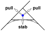
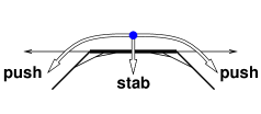
(a) (b)

Figure 6: Events for a point moving around a polygon. (a) Maintaining the active triangle. (b) Maintaining a separating edge.

Despite its good performance, the KDS just described is somewhat wasteful. Only the inner edge of the active triangle separates the moving point from the polygon, so why worry about the other two edges? This observation motivates the following lazy variant of our KDS, which has exactly the same performance bounds as Theorem 5.1 in the worst case, but is likely to be more efficient in practice.

Instead of a triangle, we maintain a single separating edge $e_{i}$ of some envelope $Q_{i}$. We update the separating edge only when $p$ passes through the line containing $e_{i}$. Again, there are two types of events: if $p$ hits the edge $e_{i}$, we have a stab event, and otherwise, we have a push event. See Figure 6(b). Stab events are handled exactly as in the previous structure: first check for a real collision, and if no collision has occurred, find a new separating edge at a deeper level in the hierarchy. After a push event, one of the edges of $Q_{i}$ adjacent to $e_{i}$, say $e^{\prime}_{i}$, is now a separating edge. However, the structure of the hierarchy ensures that $e^{\prime}_{i}$ is actually a subset of an edge $e_{j}$ of some coarser envelope $Q_{j}$; we take $e_{j}$ to be the new separating edge.

5.2 Two Translating Polygons

Now consider the case of two convex polygons $P$ and $Q$ which are translating along algebraic paths. It suffices to consider the case where $Q$ is fixed and only $P$ moves. Detecting collisions between $P$ and $Q$ is equivalent to detecting collisions between a single moving point and the static Minkowski sum $P\oplus(-Q)$, so the bounds in Theorem 5.1 immediately applies to the case of two translating polygons.

This structure is unsatisfactory, however, since it requires us to construct a decomposition of the Minkowski sum $P\oplus(-Q)$. If we want to collisions among several convex $n$-gons using this approach, we need $O(n)$ space for every active pair of polygons. In this section, we describe a modification of our previous data structures that use a separate hierarchy for each polygon, so that we only need $O(n)$ space for each polygon, plus constant space for every active pair.

Our first approach is to maintain the active cell $c$ of the mixed hierarchy of $P\oplus(-Q)$ containing the current configuration point. Whenever the configuration point leaves $c$, we can compute the new active cell $c^{\prime}$ in $O(\log\mu)$ time (Lemma 4.3). We emphasize that it is not necessary to construct the entire mixed hierarchy explicitly, but only separate hierarchies for the two polygons. If we build the mixed hierarchy out of the Dudley hierarchies of $P$ and $Q$, convex translation can now cause $O(\mu)$ events. If we use compass hierarchies instead, convex translation causes only $O(\log\mu)$ events, but the event bound for more general translations goes up to $O(\mu\log\mu)$. As in the one-point case, the event bounds also bound the total update time.

Theorem 5.2

As $P$ and $Q$ translate algebraically, we can maintain a separation certificate maintained in $O(\log(\min\{n,D/s\})$ time per event, using $O(n)$ space and preprocessing time per polygon plus $O(1)$ extra space for the pair. Both the number of events and the total update time is $O(\log\mu)$ if $P$ moves along a convex curve relative to $Q$ and $O(\mu)$ otherwise.

We can also achieve these bounds with a suitable modification of our lazy KDS. Let $P_{0},P_{1},\dots$ be a boomerang hierarchy for $P$, and $Q_{0},Q_{1},\dots$ a boomerang hierarchy for $Q$. As the polygons move, we maintain a separation certificate $(e_{i},v_{i})$, where $e_{i}$ is an edge of $Q_{i}$ and $v_{i}$ is the closest vertex of $P_{i}$ to $\mathord{\leftarrow}\mkern-6.0mu\cleaders\hbox{$\mkern-2.0mu\mathord{-}\mkern-2.0mu$}\hfill\mkern-6.0mu\mathord{\rightarrow}$ $\hfil\displaystyle{e_{i}}\hfil$ (the line through $e_{i}$), or vice versa. We always use features of the same level in both hierarchies. Given a valid separation certificate $(e_{i},v_{i})$, we can compute either a finer certificate $(e_{i+1},v_{i+1})$ or a coarser certificate $(e_{i-1},v_{i-1})$ in constant time, if one exists, by checking local neighborhoods of $e_{i}$ and $v_{i}$.

The separation certificate expires when $v_{i}$ crosses $\mathord{\leftarrow}\mkern-6.0mu\cleaders\hbox{$\mkern-2.0mu\mathord{-}\mkern-2.0mu$}\hfill\mkern-6.0mu\mathord{\rightarrow}$ $\hfil\displaystyle{e_{i}}\hfil$ . As before, there are two types of events; see Figure 7(a). (In the following description, we will assume without loss of generality that $v_{i}\in P_{i}$.)

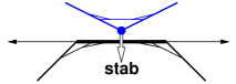
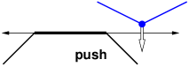
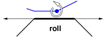
  (a) (b)

Figure 7: Events for two polygons undergoing (a) translation and (b) rotation.

To handle a stab event, where $v_{i}$ hits $e_{i}$, we refine both envelopes one level at a time until they are disjoint. (Since a single refinement may introduce a zero-length edge at $v_{i}$, we may have to refine by more than one level.) If $P_{j}$ and $Q_{j}$ are the coarsest disjoint envelopes, then either the edge of $Q_{j}$ containing $e_{i}$ or an edge of $P_{j}$ containing $v_{i}$ is a new separating edge. If $v_{i}$ is actually a vertex of $P$ and it hits the edge of $Q$ containing $e_{i}$, we report a collision.

After a push event, where $v_{i}$ does not hit the edge $e_{i}$, either an edge of $Q_{i}$ adjacent to $e_{i}$ or an edge of $P_{i}$ adjacent to $v_{i}$ is a separating edge between $P_{i}$ and $Q_{i}$ (or possibly both), depending on which has the higher slope. After updating the separation certificate, we coarsen the envelopes one level at a time, computing a new separation certificate at each new level, until the next coarser envelopes intersect.

Since we can refine or coarsen by one level in constant time, the total cost of either event is $O(\log\mu)$. The number of events is the same as for the mixed-hierarchy structure.

5.3 Rigid Motion

Now suppose $P$ and $Q$ are also allowed to rotate. As we mentioned earlier, the mixed hierarchy changes as the polygons rotate. If the active cell in the mixed hierarchy disappears due to a page turn, we can construct the new active cell in $O(\log\mu)$ time. Since we only maintain the active cell, page turns elsewhere in the mixed hierarchy cost us nothing. We do not have to worry about collapse events, since the configuration point will be ’squeezed out’ of the cell before it finishes collapsing.

Our lazy two-hierarchy data structure can now encounter an additional event, called a roll, when one of the edges adjacent to $v_{i}$ becomes parallel to $e_{i}$; see Figure 7(b). To handle a roll event, we keep $e_{i}$ as the separating edge, but now its nearest neighbor in the other envelope is a vertex adjacent to $v_{i}$. After we update the separation certificate, we then coarsen the envelopes as much as possible in $O(\log\mu)$ time, just as for a push event.

For both approaches, we have the following bounds, if we use the Dudley hierarchy; the event bound for the compass hierarchy is slightly weaker.

Theorem 5.3

As $P$ and $Q$ undergo algebraic rigid motion, we can maintain a separation certificate in $O(\log(\min\{n,D/s\})$ time per event, using $O(n)$ space and preprocessing time per polygon, plus $O(1)$ space for the pair. Both the number of events and the total update time are $O(\mu^{2})$.

5.4 Summary

Table 1 summarizes the event bounds for our kinetic data structures for various types of objects, classes of motion, and boomerang hierarchies.

Motion Compass Dudley One point, one polygon convex $O(\log\mu)$ $O(\log\mu)$ general $O(\mu\log\mu)$ $O(\mu)$ Two polygons convex translation $O(\log\mu)$ $O(\mu)$ general translation $O(\mu\log\mu)$ $O(\mu)$ rigid motion $O(\mu^{2}\log^{2}\mu)$ $O(\mu^{2})$

Table 1: The number of events and total update times of our KDSs, for different types of objects, motions, and boomerang hierarchies. Here, $\mu=\min\{n,\sqrt{D/\sigma}\}$, where $D$ is the objects’ maximum diameter and $\sigma$ is their minimum separation.

6 Inflation, Hysteresis, and Path-Sensitivity

By further modifying the lazy variants of the kinetic data structures described in the previous section, we can obtain data structures that exhibit hysteresis: after any event, the configuration must change by a certain amount before the next event occurs. Hysteresis allows us to derive upper bounds on the number of events based on geometric properties of the path that, unlike our earlier results, do not depend on smoothness or algebraicity.

For any convex polygon $P$ and real number $\varepsilon>0$, the (outer) offset polygon $P[\varepsilon]$ is a convex polygon obtained by moving each edge of $P$ outwards by a distance of $\varepsilon$ and moving the vertices along their angle bisectors. That is, each edge of $P[\varepsilon]$ is parallel to an edge of $P$ and vice versa, and the distance between their two lines is $\varepsilon$. For any point $p$ on $P[\varepsilon]$, we have $\varepsilon\leq d(p,P)\leq\varepsilon/\sin(\theta/2)$, where $\theta$ is the minimum internal angle at any vertex of $P$. Zero-length edges in $P$ induce positive-length edges in $P[\varepsilon]$.

As in the previous section, we first consider the special case of a single point $p$ moving around a polygon $Q$. Let $Q_{0},Q_{1},\dots$ be the Dudley hierarchy of $Q$, and let $\varepsilon_{i}=\alpha D/2^{i}$, the approximation error of $Q_{i}$ given by Lemma 3.3(a). (We can obtain similar results using a Dudley hierarchy instead.) We define an inflated hierarchies $Q^{\prime}_{0},Q^{\prime}_{1},\dots$, where $Q^{\prime}_{i}=Q_{i}[\varepsilon_{i}]$. See Figure 8 (but ignore the dashed edges for now). Since $Q_{0}$ is a rectangle, no envelope $Q_{i}$ has an acute vertex angle, so $d(Q^{\prime}_{i},Q)\leq(1+\sqrt{2})\varepsilon_{i}$.

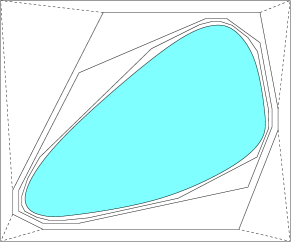
Figure 8: An inflated hierarchy. Only the outermost level of (dashed) connecting edges is shown. (Compare with Figure 1.)

As the point moves, we maintain a separating edge $e$ of some uninflated envelope $Q_{i}$. The separation certificate expires when $p$ crosses the line $\mathord{\leftarrow}\mkern-6.0mu\cleaders\hbox{$\mkern-2.0mu\mathord{-}\mkern-2.0mu$}\hfill\mkern-6.0mu\mathord{\rightarrow}$ $\hfil\displaystyle{e}\hfil$ . To compute the new separation certificate, we find the index $j$ such that $p$ lies outside $Q^{\prime}_{j}$ but inside $Q^{\prime}_{j-1}$. For the new separating edge, we take the edge of $Q_{j}$ parallel to the edge of $Q^{\prime}_{j}$ that intersects $\mathord{\leftarrow}\mkern-6.0mu\cleaders\hbox{$\mkern-2.0mu\mathord{-}\mkern-2.0mu$}\hfill\mkern-6.0mu\mathord{\rightarrow}$ $\hfil\displaystyle{e}\hfil$ . To keep the required space down to $O(n)$, we cannot precompute the breakpoints; instead, we compute each breakpoint $\vbox{\halign{#\cr$\mathord{\leftarrow}\mkern-6.0mu\cleaders\hbox{$\mkern-2.0mu\mathord{-}\mkern-2.0mu$}\hfill\mkern-6.0mu\mathord{\rightarrow}$\crcr\kern-1.0pt\nointerlineskip\cr$\hfil\displaystyle{e}\hfil$\crcr}}\cap Q^{\prime}_{j}$ on the fly in $O(j)$ time when we need it. The total cost of an event is $O(\log\mu)$, and the total number of events is the same as for the uninflated compass hierarchy.

Alternately, we can connect successive levels in the inflated hierarchy, as shown by the dashed edges in Figure 8, decomposing $Q_{0}^{\prime}\setminus Q$ into a complex of triangles and trapezoids. Each cell in this complex has one inner edge and two or three outer edges. After any event, we locate the cell $c$ in the inflated complex containing $p$; if the inner edge of $c$ is an edge of $Q^{\prime}_{j}$, we take the corresponding edge of $Q_{j}$ to be the new separating edge. The update time and number of events is the same as above.

Lemma 6.1

After any event, if $d(P,Q)=\Omega(D/n)$, then $P$ must move at least $d(P,Q)/\beta$ before the next event, where $\beta=2(1+\sqrt{2})\approx 4.8284$.

The only time we do not obtain hysteresis is when the new separating edge is an edge of the actual polygon $Q$, or equivalently, when the point $p$ lies inside the polygonal annulus $Q[\varepsilon]\setminus Q$ for some $\varepsilon=O(D/n)$.

For any real $\kappa>1$, say that a circle $C$ is $\kappa$-clear if its radius is at most $1/\kappa$ times the distance from its center to the polygon $Q$. A $\kappa$-clear decomposition of a path $\pi$ is a decomposition of $\pi$ into contiguous segments $\pi_{1},\pi_{2},\dots,\pi_{k}$, such that each segment $\pi_{i}$ is contained in a $\kappa$-clear disk. The size of such a decomposition is the number of segments.

Theorem 6.2

If $p$ moves along a path $\pi$ whose minimum distance to $Q$ is $\Omega(D/n)$, then the number of events is at most the size of the smallest $\kappa$-clear decomposition of $\pi$, where $\kappa=2\beta+1=5+4\sqrt{2}\approx 10.6569$.

The constants $\beta$ and $\kappa$ are function of the minimum external angle of any envelope and the ratio $\varepsilon_{i}/\varepsilon_{i-1}$. By using more complicated bounding polygons as the outermost level of the hierarchy, and by letting the inflation offset grow more slowly, we can decrease $\beta$ arbitrarily close to $1$ and $\kappa$ arbitrarily close to $3$. Somewhat paradoxically, however, these modifications increase both the update time per event and the worst-case number of events. In particular, using an inflated Dudley hierarchy instead of an inflated compass hierarchy doubles the value of $\beta$, even though it leads to asymptotically fewer events in the worst case.

For the case of two translating polygons $P$ and $Q$, we construct separate inflated hierarchies for both $P$ and $Q$ and use a technique similar to the lazy structure in Section 5.2. The separation certificate consists of an vertex $v$ of $P_{i}$ and an edge $e$ of $Q_{i}$, or vice versa, for some $i$. When $v$ hits $e$, we compute a new separation certificate based on which inflated envelope $Q^{\prime}_{j}$ contains the vertex $v$. The resulting structure exhibits hysteresis and path-sensitivity (with different constants $\beta$ and $\kappa$) and still satisfies Theorem 5.2.

Finally, a further modification gives us rotational hysteresis as well. That is, after any event, $P$ must either move a distance of $\Omega(d(P,Q))$ or rotate by an angle of $\Omega(d(P,Q))$ relative to $Q$ before the next event occurs. This modification requires a lower bound on the external angles of any envelope, so we can use only the compass hierarchy, not the Dudley hierarchy. Rotational hysteresis implies that the number of events is bounded by the size of a $\kappa$-clear decomposition of the path that the polygons traverse through the three-dimensional configuration space, for some constant $\kappa$.

We omit further details from this version of the paper.

7 Conclusions and Open Problems

As we mentioned in the introduction, we do no foresee any major obstacles to generalizing the two-dimensional results in this paper to three dimensions. We already have a few preliminary results, which we plan to develop further in the full paper. Generalizations of both the compass hierarchy and the Dudley hierarchy are easy to define, and at least the Dudley hierarchy provides good approximation bounds. After constructing the Dudley hierarchy of two polyhedra, we can maintain a separation certificate in $O(\operatorname{polylog}(D/s))$ time per event, using an approach similar to the lazy structure in Section 5. The number of events is $O(\mu^{2})$ for algebraic translation, and $O(\mu^{4})$ for algebraic rigid motion.

Returning to our two-dimensional results, for various measures of kinetic efficiency, we have KDSs with good performance under that measure, but only at the expense of some other kinetic quality. It would be desirable to find a single KDS that uses only linear space per polygon, has good event bounds under all three classes of motion (convex translation, algebraic translation, and algebraic rigid motion), and exhibits both translational and rotational hysteresis.

Finally, we intend to work on extending the two body methods (narrow phase) of this paper to multiple moving convex polytopes. This will require a kinetic structure that implements the broad phase of collision detection and determines which pairs of objects need to be passed on to the narrow phase.

Acknowledgments: We wish to thank Julien Basch for fruitful discussions, and Pankaj Agarwal for making us aware of Dudley’s result [Dud].

References

- [1] G. Barequet, B. Chazelle, L. J. Guibas, J. S. B. Mitchell, and A. Tal. BOXTREE: A hierarchical representation for surfaces in 3D. Comput. Graph. Forum 15(3):C387–C484, 1996. Proc. Eurographics’96.
- [2] J. Basch, L. J. Guibas, and J. Hershberger. Data structures for mobile data. Proc. 8th ACM-SIAM Sympos. Discrete Algorithms, pp. 747–756, 1997.
- [3] J. Basch, J. Erickson, L. J. Guibas, J. Hershberger, and L. Zhang. Kinetic collision detection for two simple polygons. These proceedings. http://www.uiuc.edu/ph/www/jeffe/pubs/cdsimple.html.
- [4] S. Cameron. Enhancing GJK: Computing minimum and penetration distance between convex polyhedra. Proc. Internat. Conf. Robotics and Automation, pp. 3112–3117, 1997.
- [5] K. Chung and W. Weng. Quick collision detection of polytopes in virtual environments. Proc. 3rd ACM Sympos. Virtual Reality Software and Technology, pp. 125–132. 1996.
- [6] D. Dobkin, J. Hershberger, D. Kirkpatrick, and S. Suri. Implicitly searching convolutions and computing depth of collision. Proc. 1st Annu. SIGAL Internat. Sympos. Algorithms, pp. 165–180. Lecture Notes Comput. Sci. 450, Springer-Verlag, 1990.
- [7] D. P. Dobkin and D. G. Kirkpatrick. Fast detection of polyhedral intersection. Theoret. Comput. Sci. 27:241–253, 1983.
- [8] R. M. Dudley. Metric entropy of some classes of sets with differentiable boundaries. J. Approx. Theory 10:227–236, 1974.
- [9] H. Fuchs, Z. M. Kedem, and B. Naylor. On visible surface generation by a priori tree structures. Comput. Graph. 14(3):124–133, 1980. Proc. SIGGRAPH ’80.
- [10] E. G. Gilbert, D. W. Johnson, and S. S. Keerthi. A fast procedure for computing the distance between complex objects. Internat. J. Robot. Autom. 4(2):193–203, 1988.
- [11] S. Gottschalk, M. C. Lin, and D. Manocha. OBB-tree: A hierarchical structure for rapid interference detection. Proc. SIGGRAPH ’96, pp. 171–180, 1996.
- [12] L. J. Guibas. Kinetic data structures: A state of the art report. To appear in Proc. 3rd Workshop on Algorithmic Foundations of Robotics, 1998.
- [13] J. Hershberger and S. Suri. A pedestrian approach to ray shooting: Shoot a ray, take a walk. J. Algorithms 18:403–431, 1995.
- [14] P. M. Hubbard. Collision detection for interactive graphics applications. IEEE Trans. Visualization and Computer Graphics 1(3):218–230, 1995.
- [15] J. Klosowski, H. Held, J. S. B. Mitchell, K. Zikan, and H. Sowizral. Efficient collision detection using bounding volume hierarchies of -DOPs. IEEE Trans. Visualizat. Comput. Graph. 4(1), 1998.
- [16] M. C. Lin. Efficient Collision Detection for Animation and Robotics. Ph.D. thesis, Dept. Elec. Engin. Comput. Sci., Univ. California, Berkeley, CA, 1993.
- [17] M. C. Lin and J. F. Canny. Efficient algorithms for incremental distance computation. Proc. IEEE Internat. Conf. Robot. Autom., vol. 2, pp. 1008–1014, 1991.
- [18] B. Mirtich. Impulse-based Dynamic Simulation of Rigid Body Systems. Ph.D. thesis, Dept. Elec. Engin. Comput. Sci., Univ. California, Berkeley, CA, 1996.
- [19] B. Mirtich. V-Clip: Fast and robust polyhedral collision detection. Technical Report TR-97-05, Mitsubishi Electrical Research Laboratory, 1997.
- [20] B. Mirtich and J. Canny. Impulse-based dynamic simulation. The Algorithmic Foundations of Robotics. A. K. Peters, 1995.
- [21] J. S. B. Mitchell, D. M. Mount, and S. Suri. Query-sensitive ray shooting. Proc. 10th Annu. ACM Sympos. Comput. Geom., pp. 359–368, 1994.
- [22] J. Orenstein. A comparison of spatial query processing techniques for native and parameter spaces. Proc. ACM SIGMOD Conf. on Management of Data, pp. 343–352, 1990.
- [23] R. Schneider. Convex bodies: The Brunn-Minkowski theory. Encyclopedia of Mathematics and its Applications 44. Cambridge University Press, 1993.
- [24] G. Zachmann and W. Felger. The BoxTree: Enabling real-time and exact collision detection of arbitrary polyhedra. Proc. SIVE ’95, pp. 104–113, 1995.