Incremental and Decremental Maintenance of Planar Width

Abstract

We present an algorithm for maintaining the width of a planar point set dynamically, as points are inserted or deleted. Our algorithm takes time $\mathcal{O}(kn^{\epsilon})$ per update, where $k$ is the amount of change the update causes in the convex hull, $n$ is the number of points in the set, and $\epsilon>0$ is any arbitrarily small constant. For incremental or decremental update sequences, the amortized time per update is $\mathcal{O}(n^{\epsilon})$.

1 Introduction

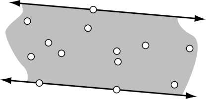
Figure 1: The width of a point set is the minimum width of an infinite strip containing the set.

The width of a geometric object is the minimum distance between two parallel supporting hyperplanes. In the case of planar objects, it is the width of the narrowest infinite strip that completely contains the object (Figure 1). The width of a planar point set can be found from its convex hull by a simple linear time “rotating calipers” algorithm that sweeps through all possible slopes, finding the points of tangency of the two supporting lines for each slope [13, 9, 16].

Despite several attempts, no satisfactory data structure is known for maintaining this fundamental geometric quantity dynamically, as the point set undergoes insertions and deletions. The methods of Janardan, Rote, Schwarz, and Snoeyink [10, 14, 15] maintain only an approximation to the true width. The method of Agarwal and Sharir [3] solves only the decision problem (is the width greater or less than a fixed bound?) and requires the entire update sequence to be known in advance. An algorithm of Agarwal et al. [1] can maintain the exact width, but requires superlinear time per update (however note that this algorithm allows the input points to have continuous motions as well as discrete insertion and deletion events). Finally, the author’s previous paper [8] provides a fully dynamic algorithm for the exact width, but one that is efficient only in the average case, for random update sequences.

In this paper we present an algorithm for maintaining the exact width dynamically. Our algorithm takes time $\mathcal{O}(kn^{\epsilon})$ per update, where $k$ is the amount of change the update causes in the convex hull, $n$ is the number of points in the set, and $\epsilon>0$ is any arbitrarily small constant. In particular, for incremental updates (insertions only) or decremental updates (deletions only), the total change to the convex hull can be at most linear and the algorithm takes $\mathcal{O}(n^{\epsilon})$ amortized time per update. For the randomized model of our previous paper, the expected value of $k$ is $\mathcal{O}(1)$ and the average case time per update of our algorithm is again $\mathcal{O}(n^{\epsilon})$.

Our approach is to define a set of objects (the features of the convex hull), and a bivariate function on those objects (the distance between parallel supporting lines), such that the width is the minimum value of this function among all pairs of objects. We could then use a data structure of the author [7] for maintaining minima of bivariate functions, however in the case of the width this minimum is more easily maintained directly. To apply this approach, we need data structures for dynamic nearest neighbor querying on subsets of features; we build these data structures by combining binary search trees with a data structure of Agarwal and Matoušek for ray shooting in convex polyhedra [2].

2 Corners and Sides

Given a planar point set $S$, we define a corner of $S$ to be an infinite wedge, having its apex at a vertex of the convex hull of $S$, and bounded by two rays through the hull edges incident to that vertex. We define a side of $S$ to be an infinite halfplane, containing $S$, and bounded by a line through one of the hull edges. Figure 2 depicts a point set, its convex hull, a corner (at the top of the figure), and a side (at the bottom of the figure).

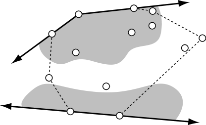
Figure 2: A corner and an incompatible side of a point set.

We say a corner and a side are compatible if they could be translated to be disjoint with one another, and incompatible otherwise. Alternatively, a side is compatible with a corner if the boundary line of the side is parallel to a different line that is tangent to the convex hull at the corner’s apex. The corner and side in the figure are incompatible, because if one translates the side’s boundary to pass through the corner’s apex, it would penetrate the convex hull.

Given a side $s$ and a compatible corner $c$, we define the distance $d(s,c)$ to be simply the Euclidean distance between the apex of the corner and the boundary line of the side. Equivalently, this is the distance between parallel lines supporting the convex hull and tangent at the two features. However, if $s$ and $c$ are incompatible, we define their distance to be $+\infty$. Let ${\rm width}(S)$ denote the width of $S$, ${\rm sides}(S)$ denote the set of sides of $S$, and ${\rm corners}(S)$ denote the set of corners of $S$.

Lemma 1

For any point set $S$ in ${\Bbb R}^{2}$,

$${\rm width}(S)=\mathop{\rm min}_{{\scriptstyle s\in{\rm sides}(S)}\atop{\scriptstyle c\in{\rm corners}(S)}}d(s,c).$$

Proof: Clearly, any compatible pair defines an infinite strip having width equal to the distance between the pair, so the overall width can be at most the minimum distance. In the other direction, let $X$ be the infinite strip tangent on both sides to the convex hull and defining the width; then at least one of the tangencies must be to a convex hull edge, for a strip tangent at two vertices could be rotated to become narrower. The opposite tangency includes at least one convex hull vertex, and the edge and opposite vertex form a compatible side-corner pair.

Lemma 2

Each side of the convex hull has at most two compatible corners. The sides compatible to a given corner of the convex hull form a contiguous sequence of the hull edges.

By Lemma 2, there are only $\mathcal{O}(n)$ compatible side-corner pairs. The known static algorithms for width work by listing all compatible pairs. The dynamic algorithm of our previous paper maintained a graph, the rotating caliper graph, describing all such pairs. However such an approach can not work in our worst-case dynamic setting: there exist simple incremental or decremental update sequences for which the set of compatible pairs changes by $\Omega(n)$ pairs after each update. Instead we use more sophisticated data structures to quickly identify the closest pair without keeping track of all pairs. To do so, we will need to keep track of the set of convex hull features, as the point set is updated.

Lemma 3 (Overmars and van Leeuwen [12])

We can maintain a list of the vertices of the convex hull of a dynamic point set in ${\Bbb R}^{2}$, and a data structure for performing logarithmic-time binary searches in the list, in linear space and time $\mathcal{O}(\log^{2}n)$ per point insertion or deletion.

Recently, Chan [5] has improved these bounds to near-logarithmic time, however this improvement does not make a difference to our overall time bound.

Lemma 4

We can maintain a dynamic point set in ${\Bbb R}^{2}$, and keep track of its sets of corners and edges, in linear space and time $\mathcal{O}(\log^{2}n+k)$ per update, where $k$ denotes the total number of corners and edges inserted and deleted as part of the update.

Proof: We apply the data structure of Overmars and van Leeuwen from the previous lemma. The set of features inserted and deleted in each update can be found by a single binary search to find one such feature, after which each adjacent feature affected by the update can be found in constant time by traversing the maintained list of hull vertices.

3 Finding the Nearest Feature

In order to apply our closest pair data structure, we need to be able to determine the nearest neighbor to each feature in a dynamic subset of other features. We first describe the easier case, finding the nearest corner to a side.

Lemma 5

We can maintain the corners of a point set in ${\Bbb R}^{2}$, and handle queries asking for the nearest corner to a given side, in time $\mathcal{O}(\log^{2}n)$ per update and $\mathcal{O}(\log n)$ per query.

Proof: We use the same dynamic convex hull data structure as in Lemma 4. Each query can be answered by a single binary search in the hull.

We next describe how to perform dynamic nearest neighbor queries in the other direction, from query corners to the nearest side. To begin with, we show how to find the nearest line to a corner, ignoring whether the line belongs to a compatible side.

Lemma 6 (Agarwal and Matoušek [2])

For any $\epsilon>0$, we can maintain a dynamic set of halfspaces in ${\Bbb R}^{3}$, and answer queries asking for the first halfspace boundary hit by a ray originating within the intersection of the halfspaces, in time $\mathcal{O}(n^{\epsilon})$ per insertion, deletion, or query.

Lemma 7

We can maintain a dynamic set of halfplanes in ${\Bbb R}^{2}$, and handle queries asking for the nearest halfplane boundary to a given query point, where the query is required to be in the intersection of the halfplanes, in time $\mathcal{O}(n^{\epsilon})$ per query, halfplane insertion, or halfplane deletion.

Proof: For a given halfplane $H$, let $D_{H}(x,y)$ denote $\pm 1$ times the distance of point $(x,y)$ to the boundary of $H$, where the factor is $+1$ for points in the halfplane and $-1$ for points outside the halfplane. $D_{H}$ is a linear function and can be used to define a three-dimensional halfspace $\{(x,y,z):D_{H}(x,y)\geq z\}$. Then $D_{H}(x,y)$ is equal to the vertical distance from point $(x,y,0)$ to the boundary of this halfspace.

Maintain such a three-dimensional halfspace for each of the halfplanes in the set, along with the data structure of Lemma 6. A nearest halfplane query from point $(x,y)$ can be answered by performing a vertical ray shooting query from point $(x,y,0)$; the first halfspace boundary hit by this ray corresponds to the nearest halfplane to the query point.

Lemma 8

We can maintain the sides of a point set in ${\Bbb R}^{2}$, and handle queries asking for the nearest side to a given corner, in amortized time $\mathcal{O}(n^{\epsilon})$ per query, side insertion, or side deletion.

Proof: We store the sides in a weight-balanced binary tree [11], according to their positions in cyclic order around the convex hull. For each node in the tree, we store the data structure of Lemma 7 for finding nearest boundaries among the sides stored at descendants of that node.

For each query, we use the binary tree to represent the contiguous group of compatible sides (as determined by Lemma 2) as the set of descendants of $\mathcal{O}(\log n)$ tree nodes. We perform the vertical ray shooting queries of Lemma 7 in the data structures stored at each of these nodes, and take the nearest of the $\mathcal{O}(\log n)$ returned sides as the answer to our query.

Each update causes $\mathcal{O}(\log n)$ insertions and deletions to the data structures stored at the nodes in the tree, and may also cause certain nodes to become unbalanced, forcing the subtrees rooted at those nodes to be rebuilt. A rebuild operation on a subtree containing $m$ sides takes time $\mathcal{O}(m^{1+\epsilon})$, and happens only after $\Omega(m)$ updates have been made in that subtree since the last rebuild, so the amortized time per update is $\mathcal{O}(n^{\epsilon})$.

4 Dynamic Width

We are now ready to prove our main result.

Theorem 1

We can maintain the width of a planar point set in ${\Bbb R}^{2}$, as points are inserted and deleted, in amortized time $\mathcal{O}(kn^{\epsilon})$ per insertion or deletion, where $k$ denotes the number of convex hull sides and corners changed by an update.

Proof: We store the data structures described in the previous lemmas, together with a pointer from each corner of the point set to the nearest side (this pointer may be null if there is no side compatible to the corner). Finally, we store a priority queue of the corner-side pairs represented by these pointers, prioritized by distance. By Lemma 1, the minimum distance in this priority queue must equal the overall width.

When an update causes a corner to be added to the set of features, we can find its nearest side in time $\mathcal{O}(n^{\epsilon})$ by Lemma 8, and add the pair to the priority queue in time $\mathcal{O}(\log n)$.

When an update causes a corner to be removed from the set of features, we need only remove the corresponding priority queue entry, in time $\mathcal{O}(\log n)$ per update.

When an update causes a side to be added to the set of features, at most two corners can be compatible with it (Lemma 2). We can find these compatible corners by binary search in the dynamic convex hull data structure used to maintain the set of features, in time $\mathcal{O}(\log n)$. For each corner, we compare the distances to the new side and the side previously stored in the pointer for that corner, and if the new distance is smaller we change the pointer and update the priority queue.

Finally, when an update causes a side to be removed, that side can be pointed to by at most the two corners compatible with it. We use the dynamic convex hull data structure to find the compatible corners, and if they point to the removed side, we recompute their nearest side in time $\mathcal{O}(n^{\epsilon})$ by Lemma 8.

Corollary 1

We can maintain the width of a point set in ${\Bbb R}^{2}$ subject to insertions only, or subject to deletions only, in amortized time $\mathcal{O}(n^{\epsilon})$ per update.

Proof: For the incremental version of the problem, each insertion creates at most two new sides and three new corners, along with deleting $h+2$ corners and $h+1$ sides where $h$ is the number of input points that become hidden in the interior of the convex hull as a consequence of the insertion. Each point can only be hidden once, so the total number of changes to the set of sides and corners over the course of the algorithm is at most $10n$. The argument for deletions is equivalent under time-reversal symmetry to that for insertions.

We note that in the average case model of our previous paper on dynamic width [8], the expected value of $k$ per update is $\mathcal{O}(1)$, and therefore our algorithm takes expected time $\mathcal{O}(n^{\epsilon})$ per update. This is not an improvement on that paper’s $\mathcal{O}(\log n)$ bound, but it is interesting that our algorithm here is versatile enough to perform well simultaneously in the incremental, decremental, and average cases.

5 Conclusions and Open Problems

We have presented an algorithm for maintaining the width of a dynamic planar point set. The algorithm can handle arbitrary sequences of both insertions and deletions, and our analysis shows it to be efficient for sequences of a single type of operation, whether insertions or deletions. Are there interesting classes of update sequences other than the ones we have studied for which the total amortized convex hull change is linear? Does there exist an efficient fully dynamic algorithm for planar width?

Another question is to what extent our algorithm can be generalized to higher dimensions. The same idea of maintaining pairwise distances between hull features seems to apply, but becomes more complicated. In three dimensions, it is no longer the case that incremental or decremental update sequences lead to linear bounds on the total change to the convex hull, but it is still true that random update sequences have constant expected change. In order to apply our approach to the three-dimensional width problem, we would need dynamic closest pair data structures for finding the face nearest a given corner, the corner nearest a given face, and the opposite edge nearest a given edge. The overall expected time per update would then be $\mathcal{O}(\log^{2}n)$ times the time per operation in these closest pair data structures. Can this approach be made to give an average-case dynamic algorithm for three dimensional width that is as good as the best known static algorithms [6, 4]?

References

- [1] P. K. Agarwal, L. J. Guibas, J. Hershberger, and E. Veach. Maintaining the extent of a moving point set. Proc. 5th Worksh. Algorithms and Data Structures, pp. 21–44. Springer-Verlag, Lecture Notes in Computer Science 1272, August 1997, http://citeseer.nj.nec.com/agarwal97maintaining.html.
- [2] P. K. Agarwal and J. Matoušek. Dynamic half-space range reporting and its applications. Algorithmica 13(4):325–345, 1995.
- [3] P. K. Agarwal and M. Sharir. Off-line dynamic maintenance of the width of a planar point set. Computational Geometry Theory & Applications 1(2):65–78, 1991.
- [4] P. K. Agarwal and M. Sharir. Efficient randomized algorithms for some geometric optimization problems. Discrete & Computational Geometry 16(4):317–337, 1996.
- [5] T. M.-Y. Chan. Dynamic planar convex hull operations in near-logarithmic amortized time. Proc. 40th Symp. Foundations of Computer Science, pp. 92–99. IEEE, October 1999.
- [6] B. Chazelle, H. Edelsbrunner, L. J. Guibas, and M. Sharir. Diameter, width, closest line pair and parametric searching. Discrete & Computational Geometry 10(2):183–196, 1993.
- [7] D. Eppstein. Dynamic Euclidean minimum spanning trees and extrema of binary functions. Discrete & Computational Geometry 13(1):111–122, 1995.
- [8] D. Eppstein. Average case analysis of dynamic geometric optimization. Computational Geometry Theory & Applications 6(1):45–68, 1996.
- [9] M. E. Houle and G. T. Toussaint. Computing the width of a set. IEEE Trans. Pattern Analysis & Machine Intelligence PAMI-10(5):761–765, 1988, http://citeseer.nj.nec.com/houle88computing.html.
- [10] R. Janardan. On maintaining the width and diameter of a planar point-set online. Int. J. Computional Geometry & Applications 3(3):331–344, 1993.
- [11] J. Nievergelt and E. M. Reingold. Binary search trees of bounded balance. SIAM J. Computing 2(1):33–43, March 1973.
- [12] M. H. Overmars and J. van Leeuwen. Maintenance of configurations in the plane. J. Comput. Sys. Sci. 23(2):166–204, 1981.
- [13] F. P. Preparata and M. I. Shamos. Computational Geometry: An Introduction. Springer-Verlag, 1985.
- [14] G. Rote, C. Schwarz, and J. Snoeyink. Maintaining the approximate width of a set of points in the plane. Proc. 5th Canad. Conf. Computional Geometry, pp. 258–263, 1993, http://citeseer.nj.nec.com/rote93maintaining.html.
- [15] C. Schwarz. Semi-dynamic maintenance of the width of a planar point set. Proc. 9th Eur. Worksh. Computational Geometry, pp. 6–9, 1993.
- [16] G. T. Toussaint. Solving geometric problems with the rotating calipers. Proc. Mediterranean Electrotechnical Conf., pp. 1–4. IEEE, 1983, http://citeseer.nj.nec.com/toussaint83solving.html.