Finite Volume Analysis of Nonlinear Thermo-mechanical Dynamics of
Shape Memory Alloys

Abstract

In this paper, the finite volume method is developed to analyze coupled dynamic problems of nonlinear thermoelasticity. The major focus is given to the description of martensitic phase transformations essential in the modelling of shape memory alloys. Computational experiments are carried out to study the thermo-mechanical wave interactions in a shape memory alloy rod, and a patch. Both mechanically and thermally induced phase transformations, as well as hysteresis effects, in a one-dimensional structure are successfully simulated with the developed methodology. In the two-dimensional case, the main focus is given to square-to-rectangular transformations and examples of martensitic combinations under different mechanical loadings are provided.

Key words: Shape memory alloys, phase transformations, nonlinear thermo-elasticity, finite volume method.

1 Introduction

The existing and potential applications of Shape Memory Alloys (SMA) lead to an increasing interest to the analysis of these materials by means of both experimental and theoretical approaches [4]. These materials have unique properties thanks to their unique ability to undergo reversible phase transformations when subjected to appropriate thermal and/or mechanical loadings. Mathematical modelling tools play an important role in studying such transformations and computational experiments, based on mathematical models, can be carried out to predict the response of the material under various loadings, different types of phase transformations, and reorientations. The development of such tools is far from straightforward even in the one-dimensional case where the analysis of the dynamics is quite involved due to a strongly nonlinear pattern of interactions between mechanical and thermal fields (e.g., [4, 18] and references therein). For a number of practical applications a better understanding of the dynamics of SMA structures with dimensions higher than one becomes critical. This makes the investigation more demanding, both theoretically and numerically.

Most results reported so far for the one-dimensional case have been obtained with the Finite Element Method (FEM) [5, 6, 24]. In addition to the challenges pertinent to coupling effects, we have to deal also with strong nonlinearities of the problem at hand. One of the approaches is to employ a FEM using cubic spline basis functions, in which case the nonlinear terms can be smoothed out by one of the available averaging algorithms. As an explicit time integration is typically employed in such situations, this results in a very small time step discretization. Seeking for a more efficient numerical approach, Melnik et al. [19, 21] used a differential-algebraic methodology to study the dynamics of martensitic transformations in a SMA rod. An extension of that approach has been recently developed in [17, 18, 22] where the authors constructed a fully conservative, second-order finite-difference scheme that allowed them to carry out computations on a minimal stencil. However, a direct generalization of the scheme to a higher dimensional case appeared to be difficult.

In this paper, we approach the same problem from the Finite Volume Method (FVM) point of view. The method is based on the integral form of the governing equations, leading to inherently conservative properties of FVM numerical schemes. The methodology is well suited for treating complicated, coupled multiphysics nonlinear problems [2, 7, 8]. It can be relatively easily generalized to higher dimensional cases. In addition to its wide-spread popularity in CFD, the method has been applied previously to linear elastic and thermoelastic problems [3, 7, 8, 14]. There are several recent results on the application of FVM to nonlinear thermo-mechanical problems and nonlinear elastic problems [2, 26]. In this paper, we develop a FVM specifically in the context of studying martensitic transformations in SMAs and demonstrate its performance in simulating the dynamical behavior of SMA rods and patches.

The paper is organized as follows. The mathematical models for the dynamics of martensitic transformations in 1D and 2D SMA structures are described in Section 2. Key issues of numerical discretization of these models, including the FVM and its computational implementation via the Differential-Algebraic Equations (DAE) approach, are discussed in Section 3. Mechanically and thermally induced transformations and hysteresis effects in SMA rods are analyzed in Section 4. Section 5 is devoted to studying nonlinear thermomechanical behavior and square-to-rectangular transformations in a SMA patch. Finally, conclusions are given in Section 6.

2 Mathematical Model for SMA Dynamics

We start our consideration from a mathematical model for the SMA dynamics based on a coupled system of the three fundamental laws, conservation of mass, linear momentum, and energy balance, in a way we described previously in [22, 18, 27]. Using these laws, the system that describes coupled thermo-mechanical wave interactions for the first order martensitic phase transformations in a three dimensional SMA structure can be written as follows [19, 22, 25]

$$\begin{array}[]{l}\displaystyle\rho\frac{\partial^{2}u_{i}}{\partial t^{2}}=\nabla_{x}\cdot\mbox{\boldmath$\sigma$}+f_{i},\quad i,j=1,2,3\\[10.0pt] \displaystyle\rho\frac{\partial e}{\partial t}-\mbox{\boldmath$\sigma$}^{T}:\nabla\mathbf{v}+\nabla\cdot\mathbf{q}=g,\end{array}$$ (1)

where $\rho$ is the density of the material, $\textbf{u}=\{u_{i}\}|_{i=1,2,3}$ is the displacement vector, v is the velocity, $\mbox{\boldmath$\sigma$}=\{\sigma_{ij}\}$ is the stress tensor, q is the heat flux, $e$ is the internal energy, $\textbf{f}=(f_{1},f_{2},f_{3})^{T}$ and $g$ are distributed mechanical and thermal loadings, respectively. Let $\phi$ be the free energy function of a thermo-mechanical system described by (1), then, the stress and the internal energy function are connected with $\phi$ by the following relationships:

$$\mbox{\boldmath$\sigma$}=\frac{\partial\phi}{\partial\mbox{\boldmath$\eta$}},\quad{e=\phi-\theta\frac{\partial\phi}{\partial\theta}},$$ (2)

where $\theta$ is the temperature, and $\eta$ the Cauchy-Lagrangian strain tensor defined as follows:

$$\eta_{ij}\left(\textrm{{x}},t\right)=\left(\frac{\partial u_{i}\left(\textrm{{x}},t\right)}{\partial x_{j}}+\frac{\partial u_{j}\left(\textbf{x},t\right)}{\partial x_{i}}\right)/2.$$ (3)

In what follows, we employ the Landau-Ginzburg form of the free energy function for both 1D and 2D SMA dynamical models [5, 9, 19]. In the 2D case, we focus our attention on the square-to-rectangular transformations that can be regarded as a 2D analog of the realistic cubic-to-tetragonal and tetragonal-to-orthorhombic transformations [12, 13]. It is known that for this kind of transformations, the free energy function $\phi$ can be constructed by taking advantage of a Landau free energy function $F_{L}$. In particular, following [12, 13, 16] (see also references therein), we have:

$$\phi=-c_{v}\theta\ln\theta+\frac{1}{2}a_{1}e_{1}^{2}+\frac{1}{2}a_{3}e_{3}^{2}+F_{L},\quad F_{L}=\frac{1}{2}a_{2}\left(\theta-\theta_{0}\right)e_{2}^{2}-\frac{1}{4}a_{4}e_{2}^{4}+\frac{1}{6}a_{6}e_{2}^{6},$$ (4)

where $c_{v}$ is the specific heat constant, $\theta_{0}$ is the reference temperature for the martensite transition, $a_{i}$, $i=1,2,3,4,6$ are the material-specific coefficients, and $e_{1}$, $e_{2}$, $e_{3}$ are dilatational, deviatoric, and shear components of strain, respectively. The latter are defined as follows:

$$e_{1}=\left(\eta_{11}+\eta_{22}\right)/\sqrt{2},\quad e_{2}=\left(\eta_{11}-\eta_{22}\right)/\sqrt{2},\quad e_{3}=\left(\eta_{12}+\eta_{21}\right)/2.$$ (5)

This free energy function $\phi$ is a convex function of the chosen order parameters when the temperature is much higher than $\theta_{0}$, in which case only austenite is stable. When the temperature is much lower than $\theta_{0}$, $\phi$ becomes non-convex and has two local minima associated with two martensite variants, which are the only stable variants. If the temperature is around $\theta_{0}$, the free energy function has totally three local minima, two of which are symmetric and associated with the martensitic phases and the remaining one is associated with the austenitic phase. In this case both martensite and austenite phases could co-exist in the system. By substituting the above free energy function into the conservation laws for momentum and energy, and using Fourier’s heat flux definition

$$q=-k\theta_{x}$$ (6)

with $k>0$ being the heat conductivity of the material, the governing equations for 2D SMA patches can be written in the following form:

$$\begin{array}[]{l}\displaystyle\rho\frac{\partial^{2}u_{1}}{\partial t^{2}}=\frac{\sqrt{2}}{2}\frac{\partial}{\partial x}\left(a_{1}e_{1}+a_{2}(\theta-\theta_{0})e_{2}-a_{4}e_{2}^{3}+a_{6}e_{2}^{5}\right)+\frac{\partial}{\partial y}\left(\frac{1}{2}a_{3}e_{3}\right)+f_{1},\\[10.0pt] \displaystyle\rho\frac{\partial^{2}u_{2}}{\partial t^{2}}=\frac{\partial}{\partial x}\left(\frac{1}{2}a_{3}e_{3}\right)+\frac{\sqrt{2}}{2}\frac{\partial}{\partial y}\left(a_{1}e_{1}-a_{2}(\theta-\theta_{0})e_{2}+e_{4}e_{2}^{3}-a_{6}e_{2}^{5}\right)+f_{2},\\[10.0pt] \displaystyle c_{v}\frac{\partial\theta}{\partial t}=k\left(\frac{\partial^{2}\theta}{\partial x^{2}}+\frac{\partial^{2}\theta}{\partial y^{2}}\right)+a_{2}\theta e_{2}\frac{\partial e_{2}}{\partial t}+g.\end{array}$$ (7)

As always, we complete system (7) by appropriate initial and boundary conditions which are problem specific (see Sections 4 and 5). As discussed before in [17, 27], the 2D model given by Eq.7 can be reduced to the Falk model in the 1D case

$$\begin{array}[]{l}\displaystyle\rho\frac{\partial^{2}u}{\partial t^{2}}=\frac{\partial}{\partial x}\left(k_{1}\left(\theta-\theta_{1}\right)\frac{\partial u}{\partial x}-k_{2}(\frac{\partial u}{\partial x})^{3}+k_{3}(\frac{\partial u}{\partial x})^{5}\right)+F,\\[10.0pt] \displaystyle c_{v}\frac{\partial\theta}{\partial t}=k\frac{\partial^{2}\theta}{\partial x^{2}}+k_{1}\theta\frac{\partial u}{\partial x}\frac{\partial v}{\partial t}+G,\end{array}$$ (8)

where $k_{1}$, $k_{2}$, $k_{3}$, $c_{v}$ and $k$ are re-normalized material-specific constants, $\theta_{1}$ is the reference temperature for 1D martensitic transformations, and $F$ and $G$ are distributed mechanical and thermal loadings.

In the subsequent sections, the above models are applied to the description of the first order martensitic transformations. While such transformations are reasonably well documented for the 1D case, only few results are known for the 2D case. In what follows, we develop a FVM to simulate the dynamics described by the models (7) and (8) and apply it in both 1D and 2D cases.

3 Numerical Algorithm

The systems (7) and (8) are analyzed numerically with the FVM implemented here with the help of the DAE approach. For the 1D case, the FVM method yields the same result as the conservative scheme already discussed in [18]. However, the approach developed here is generalized in a straightforward manner to a higher dimensional case and we demonstrate its applicability by a numerical example in the case of two spatial dimensions. First, we note that it is convenient to replace the original model (7) by a system of equivalent differential-algebraic equations as it was proposed earlier in [19, 21]:

$$\begin{array}[]{l}\displaystyle\frac{\partial e_{1}}{\partial t}=\frac{\sqrt{2}}{2}\left(\frac{\partial v_{1}}{\partial x}+\frac{\partial v_{2}}{\partial y}\right),\quad\frac{\partial e_{2}}{\partial t}=\frac{\sqrt{2}}{2}\left(\frac{\partial v_{1}}{\partial x}-\frac{\partial v_{2}}{\partial y}\right),\\[10.0pt] \displaystyle\rho\frac{\partial v_{1}}{\partial t}=\frac{\partial\sigma_{11}}{\partial x}+\frac{\partial\sigma_{12}}{\partial y}+f_{x},\quad\rho\frac{\partial v_{2}}{\partial t}=\frac{\partial\sigma_{12}}{\partial x}+\frac{\partial\sigma_{22}}{\partial y}+f_{y},\\[10.0pt] \displaystyle c_{v}\frac{\partial\theta}{\partial t}=k\left(\frac{\partial^{2}\theta}{\partial x^{2}}+\frac{\partial^{2}\theta}{\partial y^{2}}\right)+a_{2}\theta e_{2}\frac{\partial e_{2}}{\partial t}+g,\\[10.0pt] \displaystyle\sigma_{11}=\frac{\sqrt{2}}{2}(a_{1}e_{1}+a_{2}\left(\theta-\theta_{0}\right)e_{2}-a_{4}e_{2}^{3}+a_{6}e_{2}^{5}),\\[10.0pt] \displaystyle\sigma_{12}=\sigma_{21}=\frac{1}{2}a_{3}e_{3},\\[10.0pt] \displaystyle\sigma_{22}=\frac{\sqrt{2}}{2}(a_{1}e_{1}-a_{2}\left(\theta-\theta_{0}\right)e_{2}+a_{4}e_{2}^{3}-a_{6}e_{2}^{5}).\end{array}$$ (9)

This system is solved numerically together with the compatibility relation written below in terms of strains:

$$\frac{\partial^{2}e_{1}}{\partial x_{1}^{2}}+\frac{\partial^{2}e_{1}}{\partial x_{2}^{2}}-\sqrt{8}\frac{\partial^{2}e_{3}}{\partial x_{1}\partial x_{2}}-\frac{\partial^{2}e_{2}}{\partial x_{1}^{2}}+\frac{\partial^{2}e_{2}}{\partial x_{1}^{2}}=0.$$ (10)

There are eight variables in total that the problem needs to be solved for in this 2D case and there are eight equations. The equations for strains, velocities and temperature are all differential equations, complemented by stress-strain relationships which are treated as algebraic.

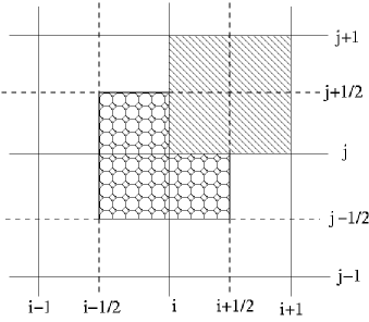
Figure 1: Staggered grid for space discretization using finite volume methods.

In what follows, we highlight the key elements of our numerical procedure based on the FVM implemented with the help of the DAE approach. First, all equations in the system (9) are discretized on a staggered grid represented schematically in Fig 1. Assuming that the entire computational domain is a rectangle with an area of $L_{x}\times L_{y}$ ${\rm cm}^{2}$, we define the spatial integer grid points $(x_{i},y_{j})$ and the spatial flux points $(\bar{x}_{i},\bar{y}_{j})$ as follows:

$$\begin{array}[]{l}\displaystyle x_{i}=ih_{x},\quad,i=0,1,2,\cdots,M,\qquad\bar{x}_{i}=(i-\frac{1}{2})h_{x},\quad,i=1,2,\cdots,M\\[10.0pt] \displaystyle y_{j}=jh_{y},\quad,j=0,1,2,\cdots,N,\qquad\bar{y}_{j}=(j-\frac{1}{2})h_{y},\quad,j=1,2,\cdots,N\end{array}$$ (11)

where $M$ and $N$ are the number of grid points such that $M\times h_{x}=L_{x}$ and $N\times h_{y}=L_{y}$, respectively. The $(i,j)$th control volume for the velocities is $[\bar{x}_{i},\bar{x}_{i+1}]\times[\bar{y}_{j},\bar{y}_{j+1}]$, as sketched by the rectangular tiled mosaic area in Fig.1, including the upper right part overlapped with the hatched area. The variables, defined in this control volume, that will be differentiated are marked by a top bar, for instance $\bar{v}_{1}(i,j)$. The control volume for the strains $e_{1}$ and $e_{2}$, temperature $\theta$, and stresses $\sigma_{11}$, $\sigma_{12}$, and $\sigma_{22}$ is given by $[x_{i},x_{i+1}]\times[y_{j},y_{j+1}]$, represented by the rectangular hatched area in Fig. 1. We refer to these variables, defined in this control volume, without a top bar, for instance $e_{1}(i,j)$ for $e_{1}$, etc.

By integrating all the differential equations over their own control volumes and assuming that all the unknowns are linear in each single control volume while being continuous and piecewise linear in the entire computational domain, the five partial differential equations are reduced to a system of ordinary differential equations. The remaining three algebraic equations of the original system are discretized directly on the grid. The result is the following system:

$$\begin{array}[]{l}\displaystyle\frac{de_{1}(i,j)}{dt}=(I_{y}D_{x}\bar{v}_{1}(i,j)+I_{x}D_{y}\bar{v}_{2}(i,j))/\sqrt{2},\\[10.0pt] \displaystyle\frac{de_{2}(i,j)}{dt}=(I_{y}D_{x}\bar{v}_{1}(i,j)-I_{x}D_{y}\bar{v}_{2}(i,j))/\sqrt{2},\\[10.0pt] \displaystyle\rho\frac{d\bar{v}_{1}(i,j)}{dt}=I_{y}D_{x}\sigma_{11}(i-1,j-1)+I_{x}D_{y}\sigma_{12}(i-1,j-1)+f_{1},\\[10.0pt] \displaystyle\rho\frac{d\bar{v}_{2}(i,j)}{dt}=I_{y}D_{x}\sigma_{12}(i-1,j-1)+I_{x}D_{y}\sigma_{22}(i-1,j-1)+f_{2},\\[10.0pt] \displaystyle c_{v}\frac{d\theta(i,j)}{dt}=k(\triangle\theta(i,j))+\frac{\sqrt{a_{2}}}{2}\theta(i,j)e_{2}(i,j)\frac{de_{2}}{dt}+g,\\[10.0pt] \displaystyle\sigma_{11}(i,j)=\frac{\sqrt{2}}{2}(a_{1}e_{1}(i,j)+a_{2}(\theta(i,j)-\theta_{0})e_{2}(i,j)-\frac{a_{4}}{4}g_{1}(i,j)+\frac{a_{6}}{6}g_{2}(i,j)),\\[10.0pt] \displaystyle\sigma_{12}(i,j)=\sigma_{21}(i,j)=\frac{1}{2}(a_{3}e_{3}(i,j)),\\[10.0pt] \displaystyle\sigma_{22}(i,j)=\frac{\sqrt{2}}{2}(a_{1}e_{1}(i,j)-a_{2}(\theta(i,j)-\theta_{0})e_{2}(i,j)+\frac{a_{4}}{4}g_{1}(i,j)-\frac{a_{6}}{6}g_{2}(i,j)).\end{array}$$ (12)

where $D_{x}$ and $D_{y}$ are the discrete difference operators in the $x$ and $y$ directions, respectively, while $I_{x}$ and $I_{y}$ are the discrete interpolation operator in the $x$ and $y$ directions, and $\triangle$ is the discrete Laplace operator. For example, for the simplest case of the first order accurate scheme, the operators $D_{x}$ and $I_{y}$ could be written as follows

$$D_{x}\bar{v}_{1}(i,j)=(\bar{v}_{1}(i,j+1)-\bar{v}_{1}(i,j))/h_{x},\quad I_{y}\bar{v}_{1}(i,j)=(\bar{v}_{1}(i,j)+\bar{v}_{1}(i+1,j))/2,$$ (13)

with similar representations for the second order accurate schemes. Moving to the time discretization procedure, it is convenient to re-write system (12) in the following vector-matrix form:

$${\bf{A}}\frac{{d{\bf{U}}}}{{dt}}+{\bf{H}}\left({t,{\bf{X}},{\bf{U}}}\right)={\bf{0}}$$ (14)

with matrix $A={\rm diag}(a_{1},a_{2},...,a_{N})$ having entries “one” for differential and “zero” for algebraic equations for stress-strain relationships, and vector-function ${\bf H}$ defined by the right hand side parts of (12). This (stiff) system is solved with respect to the vector of unknowns ${\bf U}$ that have $6\times m_{x}\times m_{y}+2\times(m_{x}+1)\times(m_{y}+1)$ components by using the second order backward differentiation formula (BDF) [11]:

$${\rm{\bf A}}\left({\frac{3}{2}{\rm{\bf U}}^{n}-2{\rm{\bf U}}^{n-1}+\frac{1}{2}{\rm{\bf U}}^{n-2}}\right)+\Delta t{\rm{\bf H}}\left({t_{n},{\rm{\bf X}},{\rm{\bf U}}^{n}}\right)=0$$ (15)

where $n$ denotes the current time layer.

This spatio-temporal discretization is applied to the analysis of phase transformations with the following modification. In order to improve convergence properties of the scheme, we employ a relaxation process connecting two consecutive time layers via a relaxation factor $\omega$ as follows:

$$y(i,j)=(1-\omega)\times y(i,j)^{n}+\omega\times y(i,j)^{n+1},$$ (16)

where the variable $y$ could be any of the following: $e_{1}(i,j)$, $e_{2}(i,j)$, $v_{1}(i,j)$, $v_{2}(i,j)$, or $\theta(i,j)$. Note that in the general case the relaxation factors need not be the same for all the variables. In the present paper, all the numerical results have been obtained using (16) with all the relaxation factors set to $0.85$.

We note that nonlinear terms in the model are averaged in the Steklov sense [18], so that for nonlinear function $f(e_{2})$ (in particular, for $e_{2}^{3}$ and $e_{2}^{5}$), averaged in the interval $[e_{2}^{n},e_{2}^{n+1}]$, we have

$$g\left(e_{2}^{n},e_{2}^{n+1}\right)=\frac{1}{e_{2}^{n+1}-e_{2}^{n}}\int_{e_{2}^{n}}^{e_{2}^{n+1}}f(e_{2})de_{2}.$$ (17)

Applying this idea to $e_{2}^{3}$ and $e_{2}^{5}$, we have:

$$\begin{array}[]{c}\displaystyle g_{1}\left(i,j\right)=\frac{\left(e_{2}^{n+1}\right)^{4}-(e_{2}^{n})^{4}}{e_{2}^{n+1}-e_{2}^{n}}=\frac{1}{4}\sum_{k=0}^{3}(e_{2}^{n+1})^{3-k}(e_{2}^{n})^{k},\\[10.0pt] \displaystyle g_{2}\left(i,j\right)=\frac{(e_{2}^{n+1})^{6}-(e_{2}^{n})^{6}}{e_{2}^{n+1}-e_{2}^{n}}=\frac{1}{6}\sum_{k=0}^{5}(e_{2}^{n+1})^{5-k}(e_{2}^{n})^{k}.\end{array}$$ (18)

where $e_{2}^{n}$ and $e_{2}^{n+1}$ stands for $e_{2}(i,j)^{n}$ and $e_{2}(i,j)^{n+1}$, respectively.

Finally, we note that in our FVM implementation the nonlinear coupling term in the energy balance equation is regarded as a time-dependent source term. In the $(i,j)$th control volume for the discretization of $\theta$, we approximate that term as follows:

$$\int_{x_{i}}^{x_{i+1}}\int_{y_{j}}^{y_{j+1}}\left(k_{1}\theta e_{2}\frac{\partial e_{2}}{\partial t}\right)dxdy\approx\theta(i,j)e_{2}(i,j)\frac{de_{2}(i,j)}{dt}.$$ (19)

As seen from (15), we use an implicit time integrator based on the BDF. At each time step we apply the bi-conjugate gradient method to solve the resultant system of algebraic equations with the Jacobian matrix updated on each iteration.

4 Dynamics of SMA Rods and Strips

We first consider a situation where the deformation of a 2D SMA sample in the $x_{1}$ direction substantially exceeds the deformation in the other direction, so that the deformation in the $x_{2}$ direction can be neglected and the sample can be treated as a SMA long strip or simply as a rod. Introducing formally $\varepsilon=\partial{u}/\partial x$ and $v=\partial{u}/\partial t$, system (8) can be recast in the following form:

$$\begin{array}[]{c}\displaystyle\frac{{\partial\epsilon}}{{\partial t}}=\frac{{\partial v}}{{\partial x}},\quad{\rho\frac{{\partial v}}{{\partial t}}=\frac{{\partial s}}{{\partial x}}+F},\\[10.0pt] \displaystyle s={k_{1}\left({\theta-\theta_{1}}\right)\epsilon-k_{2}\epsilon^{3}+k_{3}\epsilon^{5}},\\[10.0pt] \displaystyle c_{v}\frac{{\partial\theta}}{{\partial t}}=k\frac{{\partial^{2}\theta}}{{\partial x^{2}}}+k_{1}\theta\epsilon\frac{{\partial v}}{{\partial x}}+G,\end{array}$$ (20)

where $\epsilon$ is strain and $s$ is stress.

The numerical procedure described in Section 3 is applied here to the solution of system (20). It is aimed at the analysis of martensitic transformations in the SMA rod, including hysteresis effects during the transformations. Computational experiments reported in this section were performed for a $Au_{23}Cu_{30}Zn_{47}$ rod with a length of $L=1$ ${\rm cm}$ and all parameter values found in [9, 20, 24], in particular:

$$\begin{array}[]{c}\displaystyle k_{1}=480\,g/ms^{2}cmK,\qquad k_{2}=6\times 10^{6}g/ms^{2}cmK,\qquad k_{3}=4.5\times 10^{8}g/ms^{2}cmK,\\[10.0pt] \displaystyle\theta_{1}=208K,\quad\rho=11.1g/cm{}^{3},\quad C_{v}=3.1274g/ms^{2}cmK,\quad k=1.9\times 10^{-2}cmg/ms^{3}K.\end{array}$$

The boundary conditions for $u$ and $\theta$ for all the numerical experiments reported in this section are:

$$\begin{array}[]{c}\displaystyle u(0,t)=u_{L}(t),\quad u(L,t)=u_{R}(t),qquad\frac{\partial\theta}{\partial x}(0,t)=\theta_{L}(t),\quad\frac{\partial\theta}{\partial x}(L,t)=\theta_{R}(t)\end{array}$$ (21)

with given functions $u_{i}(t)$ and $\theta_{i}(t)$, $i=L,R$ and corresponding conditions for the velocities.

In the numerical experiments reported below, we used only $9$ nodes for the velocity discretization (and 8, excluding boundaries, for the rest of variables). The time stepsize in all the experiments was set to $\tau=1.\times 10^{-4}$. All the simulations were performed for the time period $[0,24]$ which spans two periods of the loading cycle.

4.1 Mechanically Induced Transformations and Hysteresis

The first numerical experiment deals with the case of mechanical loading in the low-temperature regime. The initial conditions for this computational experiment are defined by the following configuration of martensites ([15, 20, 22]):

$$\theta(x,0)=220,\qquad u_{0}=\left\{\begin{array}[]{l}0.11869x,\qquad\qquad 0\leq x\leq 0.25\\ 0.11869(0.5-x),\quad 0.25\leq x\leq 0.75\\ 0.11869(x-1),\qquad 0.75\leq x\leq 1\end{array}\right.,v^{0}=u^{1}=0$$ (22)

with the time varying distributed mechanical loading defined as

$$F=7000\sin^{3}\left(\frac{\pi t}{2}\right)\,\,g/\left(ms^{2}cm^{2}\right),\,\,\,\,G=0.$$ (23)

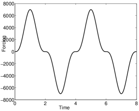
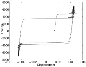
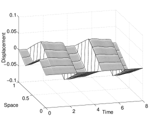
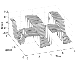
Figure 2: Mechanical induced phase transformation and mechanical hysteresis in SMA rod.

Under the given distributed mechanical loading, the SMA rod is expected to switch between different combinations of the martensite variants, and a hysteresis loop must be observed similar to those reported for ferroelastic materials at low temperature. In Fig. 2 we present simulation results for this case. The mechanical hysteresis is obtained by plotting displacement $u$ as a function of $F$ at $x=3/8$cm (the upper right plot). The time-varying mechanical loading for this case is plotted in the upper left plot. The simulated strain and the displacement distribution are also plotted as functions of time and space (lower plots). The combination of martensitic variants is changing with time-dependent mechanical loading and no stable austenite is observed at this low temperature.

Our next goal is to analyze the behavior of the same SMA rod under a medium temperature where both martensite and austenite phases may co-exist. The following initial conditions will allow us to start from the austenitic phase:

$$\theta(x,0)=250,\,\,u_{0}=0,\,\,\,v^{0}=u^{1}=0.$$ (24)

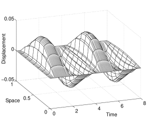
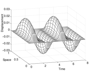
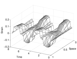
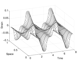
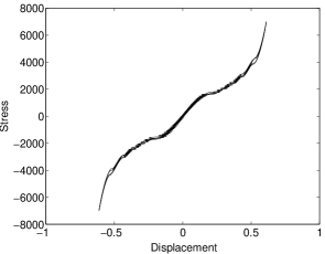
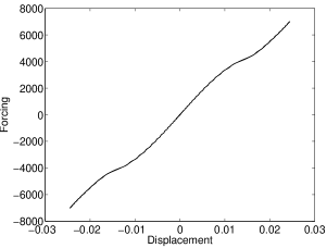
Figure 3: Dynamics and mechanical hysteresis of SMA at medium and high temperature

The boundary conditions as well as mechanical and thermal loadings in this case are kept identical the previous experiment. In this case, the free energy function has three minima that correspond to two martensites and one austenite. The numerical results for this case are presented in the left column of Fig.3. It is observed that when the applied loading exceeds a certain value, the austenite is transformed to a combination of martensitic variants. The reverse transformation is taken place when the loading changes its sign. In contrast to the results presented in Fig. 2, we observe that the wide hysteresis loop, typical for the low temperature case, disappears.

If we increase the initial temperature further to $\theta(x,0)=300$, the free energy function becomes convex and has only one minimum associated with the austenite phase. During the entire loading cycle, no martensite is expected under these thermal conditions. The dynamics of the SMA rod in this case exhibits nonlinear thermomechanical behaviour without phase transformations. This is confirmed by the numerical results presented in the right column of Fig.3.

4.2 Thermally induced Phase Transformations and Hysteresis

Thermally induced martensitic phase transformations and thermal hysteresis in SMA rods can be analyzed with the same model under time-dependent thermal loading conditions. Indeed, let us choose the initial conditions as follows:

$$\theta(x,0)=230,\,\,u_{0}=\left\{\begin{array}[]{l}0.11869x,\qquad\qquad 0\leq x\leq 0.5\\ 0.11869(1-x),\quad 0\leq x\leq 0.5\end{array}\right.,v^{0}=u^{1}=0$$

The boundary conditions remain the same as in the previous computational experiment, but the loadings conditions now become:

$$G=600\sin\left(\frac{\pi t}{6}\right)\,\,g/\left(ms^{3}cm\right),\,\,\,F=500\,g/\left(ms^{2}cm^{2}\right).$$

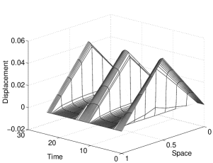
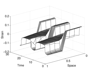
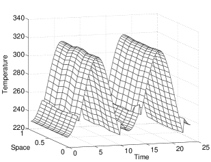
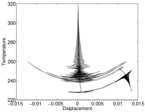
Figure 4: Thermally induced phase transformation and thermal hysteresis in SMA rod.

Numerical results for this case are presented in Fig.4. Analyzing strain and displacement distributions, we observe that the combination of martensitic variants is transformed into the austenite phase when the temperature exceeds a certain value. The reverse process is taken place when the temperature decreases, passing the critical threshold. Note that due to the presence of thermal hysteresis, the critical temperature value for the martensite-to-austenite transformation is different from that of the austenite-to-martensite transformation. A schematic representation of the observed thermal hysteresis is given in the lower right part of Fig. 4 where we presented the temperature at $x=3/8$ as a function of strain at the same spatial point.

5 Dynamics of SMA Patches

The situation becomes more involved for 2D structures. Experimental, let alone numerical, results for this situation are scarce [27]. In order to apply the FVM to the 2D model discussed in Section 2, we chose the same material as before, assuming that $a_{2}=k_{1},a_{3}=k_{2},\,a_{4}=k_{3},a_{1}=k_{1},\,a_{3}=2k_{1}$ and therefore effectively linking parameters in model (7) and model (8).

5.1 Nonlinear Thermomechanical Behavior

The first numerical experiment on a SMA patch is aimed at the analysis of the dynamical thermo-mechanical response of the patch to a varying distributed mechanical loading, too small to induce any phase transformations. The initial temperature of the patch is set to $250^{o}$ while all other variables are set initially to zero. Conditions at the boundaries are:

$$\begin{array}[]{l}\displaystyle\frac{\partial\theta}{\partial x}=0,\quad\frac{\partial u_{2}}{\partial x}=0,\quad u_{1}=0,\quad\textrm{on left and right boundaries},\\[10.0pt] \displaystyle\frac{\partial\theta}{\partial y}=0,\quad\frac{\partial u_{1}}{\partial y}=0,\quad u_{2}=0,\quad\textrm{on top and bottom boundaries}.\end{array}$$ (25)

Similarly, the mechanical boundary conditions are enforced in terms of velocity components. The loading conditions in this experiment are:

$$f_{1}=200\sin(\pi t/6){\textrm{g}}/(\textrm{ms}^{2}\textrm{cm}^{2}),\quad f_{2}=200\sin(\pi t/40){\textrm{g}}/(\textrm{ms}^{2}\textrm{cm}^{2}).$$

The time span for this simulation, $[0,24]$, covers two periods of loading. The time stepsize is set to $1\times 10^{-4}$. We take $15$ nodes used in each direction. The dimensions of the SMA patch are taken as $1\times 0.4$ ${\rm cm}^{2}$.

The variations in the displacements $u_{1}$, $u_{2}$ , deviatoric strain $e_{2}$, and the temperature $\theta$ along the line $y=0.2\rm{cm}$ (the central horizontal line) as functions of time are presented in Fig.5. These simulations show that both thermal and mechanical fields are driven periodically by the distributed mechanical loading. Under such a small loading, the SMA patch behaves just like a conventional thermoelastic material. Observed oscillations are due to nonlinear thermomechanical coupling, but no phase transformations are observed in this case.

5.2 Phase Transformations in SMA Patches

Our aim in this section is to analyze spatio-temporal patterns of martensitic transformations in a 2D SMA patch. The SMA patch, used in this computational experiment, is made of the same material as before. The patch is assumed square in shape with dimensions $1\times 1$ ${\rm cm}^{2}$. The initial temperature distribution is set to $\theta^{0}=240^{o}$, and all other variables are initially set to zero. The boundary conditions are homogeneous and

$$\frac{\partial\theta}{\partial n}=0,\quad u_{2}=u_{1}=0,\quad\textrm{on all the four boundaries,}$$ (26)

where n is the unit normal vector. We apply the following loading to the sample, specified below for one period:

$$f_{1}=f_{2}=6000\left\{\begin{array}[]{llll}\sin(\pi t/3),&0\leq t\leq 4,\\ 0,&4\leq t\leq 6,\\ \sin(\pi(t-2))/3),&6\leq t\leq 10,\\ 0,&10\leq t\leq 12.\\ \end{array}\right.$$ (31)

The numerical results for this case are presented in Fig.6 where the values of ”y” are taken in the middle of the sample. The spatio-temporal plot of the order parameter $e_{2}$ demonstrates a periodicity pattern in the observed phase transformations due to periodicity of the loading. It is observed also that the temperature oscillates synchronously with the mechanical field variables due to the thermo-mechanical coupling.

As we mentioned earlier, there are two martensitic variants in the square-to-rectangular transformations. The following analysis proves to be useful in validating the results of computational experiments. Assuming the temperature difference $d\theta=\theta-\theta_{0}$, one can easily calculate the deviatoric strain that corresponds to the austenite and martensite variants by minimizing the Landau free energy functional. In particular from the condition $\partial{F_{l}}/\partial{e_{2}}=0$ we get:

$$e_{2}=0;\quad e_{2}^{2}=\frac{a_{4}\pm\sqrt{a_{4}^{2}-4a_{2}d\theta a_{6}}}{2a_{6}}.$$

The value $e_{2}=0$ corresponds to the austenitic phase. If we denote $(a_{4}+\sqrt{a_{4}^{2}-4a_{2}d\theta a_{6}})/2a_{6}$ by $e_{m}$, then $e_{2+}=+\sqrt{e_{m}}$ or $e_{2-}=-\sqrt{e_{m}}$ are the strains that correspond to the two martensite variants. We call them martensite plus and martensite minus, respectively. If we take $d\theta=42^{o}$, then for the material considered here we can estimate that $e_{2+}=0.12$ and $e_{2-}=0.12$. This provides a fairly good estimate for the 1D case. However, as was pointed out in [13, 16], for the 2D case such an estimate can be adequate only in homogenous cases. Although the quality of this estimate is dependent on the boundary conditions for a specific problem, this estimate proves to be a reasonable initial approximation to the deviatoric strain.

In Fig. 7 we present two snapshots (at $t=2$ and $t=8$) of the spatial distributions of $e_{2}$ and $\theta$. It is observed that when the mechanical loading achieves its (positive) maximum, the SMA patch is divided into two sub-domains determined by the deviatoric strain, as seen from the $e_{2}$ plot at $t=2$. In the upper-left triangular-shape area, the simulated deviatoric strain corresponds to the martensite plus, while on the opposite side, the deviatoric strain corresponds to the martensite minus. At $t=8$, when the mechanical loading changes its sign to the opposite, the martensitic transformation is observed again, but now in the reverse direction. The second period of loading confirms these observations.

6 Conclusion

In this paper, we developed a finite volume methodology for the analysis of nonlinear coupled thermomechanical problems, focusing on the dynamics of SMA rods and patches. Both mechanically and thermally induced phase transformations, as well as hysteresis effects, in one-dimensional structures are successfully simulated. While these results can be obtained with the recently developed conservative difference schemes, their generalization to higher dimensional cases is not trivial. In this paper, we also highlighted the application of the developed FVM to the 2D problems focusing on square-to-rectangular transformations in SMA materials demonstrating practical capabilities of the developed methodology.

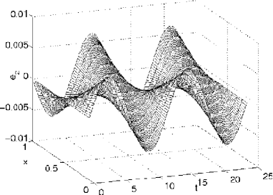
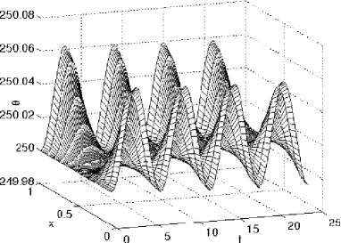
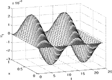
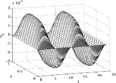
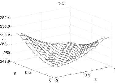
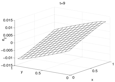
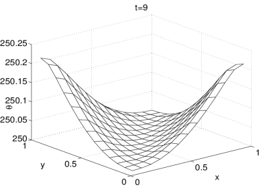
Figure 5: Thermo-mechanical waves in SMA patches caused by varying mechanical loadings.

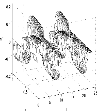
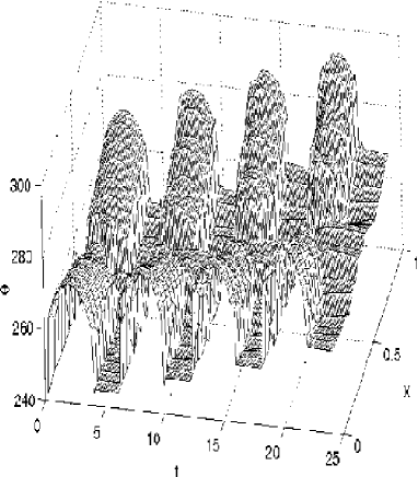
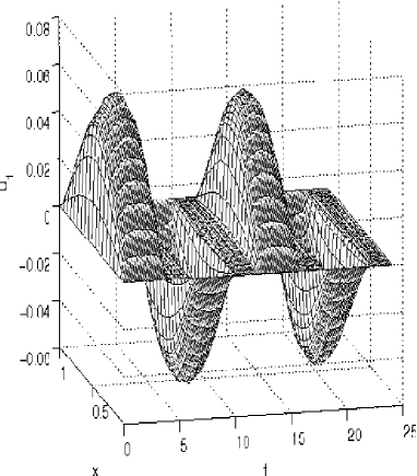
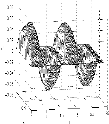
Figure 6: Martensitic transformation in a square SMA patch caused by mechanical loadings in the $x$ and $y$ direction.

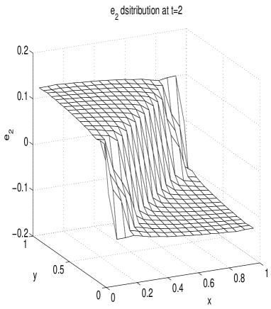
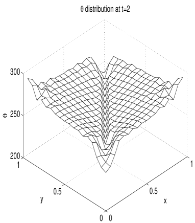
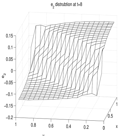
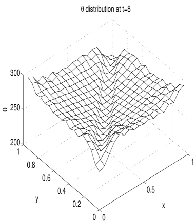
Figure 7: Martensite combinations and temperature distributions in a square SMA patch after phase transformations caused by mechanical loadings in the $x$ and $y$ direction.

References

- [1]
- [2] Berezovski A and Maugin GA (2003) Simulation of wave and front propagation in thermoelastic materials with phase transformation. Computational Materials Science28: 478-48
- [3] Berezovski A and Maugin GA (2001) Simulation of Thermoelastic Wave Propagation by Means of a Composite Wave-Propagation Algorithm. Journal of Computational Physics 168: 249-264A.
- [4] Birman V (1997) Review of mechanics of shape memory alloys structures. Appl.Mech.Rev. 50: 629-645.
- [5] Bubner N (1996) Landau-Ginzburg model for a deformation-driven experiment on shape memory alloys. Continuum Mech. Thermodyn. 8: 293-308.
- [6] Bubner N, Mackin G, and Rogers, RC (2000) Rate dependence of hysteresis in one-dimensional phase transitions. Computational Material Science 18: 245-254.
- [7] Demirdzic I and Muzaferija S (1994) Finite volume method for stress analysis in complex domains. International Journal for Numerical Methods in Engineering 37: 3751-3766.
- [8] Demirdzic I, Muzaferija S, and Peric M (1997) Benchmark solutions of some structural analysis problmes using finite volume method and miltigridaceleration. International Journal for Numerical Analysis in Engineering 40: 1893-1908.
- [9] Falk F (1980) Model free energy, mechanics, and thermodynamics of shape memory alloys. Acta Metallurgic 28: 1773-1780.
- [10] Falk F and Konopka P (1990) Three-dimensional Landau theory describing the martensitic phase transformation of shape memory alloys. J.Phys.:Condens.Matter. 2: 61-77.
- [11] Hairer E, Norsett SP, and Wanner G (1996) Solving ordinary differential equations II-stiff and differential algebraic problems, Springer-Verlag, Berlin.
- [12] Ichitsubo T, Tanaka K, Koiva M, and Yamazaki Y (2000) Kinetics of cubic to tetragonal transformation under external field by the time-dependent Ginzburg-Landau approach. Phys.Rev.B 62(9): 5435-5441.
- [13] Jacobs AE (2000) Landau theory of structures in tetragonal-orthorhombic ferroelastics. Phys. Rev. B 61(10): 6587-6595.
- [14] Jasak H, Weller HG (2000) Application of the finite volume method and unstructured meshes to linear elasticity. Int.J.Numer.Meth.Engng. 48: 267-287.
- [15] Klein K (1995) Stability and uniqueness results for a numerical approximation of the thermomechanical phase transitions in shape memory alloys. Advances in Mathematical Sciences and Applications (Tokyo) 5(1): 91-116.
- [16] Lookman T, Shenoy SR, Rasmusseh, KO, Saxena A, and Bishop AR (2003) Ferroelastic dynamics and strain compatibility. Physical Review B 67: 024114.
- [17] Matus P, Melnik RVN, Rybak IV (2003) Fully conservative difference schemes for nonlinear models describing dynamics of materials with shape memory. Dokl. of the Academy of Science of Belarus 47: 15-18.
- [18] Matus P, Melnik RVN, Wang L, Rybak I (2004) Application of fully conservative schemes in nonlinear thermoelasticity: Modelling shape memory materials. Mathematics and Computers in Simulation. Mathematics And Computers in Simulation 65: 489-509.
- [19] Melnik RVN, Robert AJ, and Thomas KA (2000) Computing dynamics of Copper-based SMA via central manifold reduction models. Computational Material Science 18: 255-268.
- [20] Melnik RVN, Roberts AJ, and Thomas KA (2001) Coupled Thermomechanical dynamics of phase transitions in shape memory alloys and related hysteresis phenomena. Mechanics Research Communications 28(6): 637-651.
- [21] Melnik RVN, Roberts AJ, and Thomas KA (2002) Phase transitions in shape memory alloys with hyperbolic heat conduction and differential algebraic models. Computational Mechanics, 29(1): 16-26.
- [22] Melnik RVN, Wang L, Matus P, and Rybak I (2003) Computational aspects of conservative difference schemes for shape memory alloys applications. Computational science and its application - ICCSA 2003,PT2, LNCS 2668: 791-800.
- [23] Melnik RVN and Roberts AJ (2003) Modelling nonlinear dynamics of shape memory alloys with approximate models of coupled thermoelasticity. Z.Angew.Math. 82(2): 93-104.
- [24] Niezgodka M and Sprekels J (1991) Convergent numerical approximations of the thermomechanical phase transitions in shape memory alloys. Numerische Mathematik 58: 759-778.
- [25] Pawlow I (2000) Three dimensional model of thermomechanical evolution of shape memory materials. Control and Cybernetics 29: 341-365.
- [26] Tuzel H and Erbay HA (2004) The dynamic response of an incompressible non-linearly elastic membrane tube subjected to a dynamic extension. International Journal of Non-Linear Mechanics 39: 515-537V.
- [27] Wang L and Melnik RVN (2004) Thermomechanical waves in SMA patches under small mechanical loadings. in Lecture Notes in Computer Science 3039, M.Bubak, G.Dick, v.Albada, P.M.A.Sloot, and J.Dongarra (eds) Springer, Berlin, pp 645-652.