Solving Stochastic Differential Equations with Jump-Diffusion Efficiently: Applications to FPT Problems in Credit Risk
Abstract. The first passage time
(FPT) problem is ubiquitous in many applications. In finance, we
often have to deal with stochastic processes with jump-diffusion, so
that the FTP problem is reducible to a stochastic differential
equation with jump-diffusion. While the application of the
conventional Monte-Carlo procedure is possible for the solution of
the resulting model, it becomes computationally inefficient which
severely restricts its applicability in many practically interesting
cases. In this contribution, we focus on the development of
efficient Monte-Carlo-based computational procedures for solving the
FPT problem under the multivariate (and correlated) jump-diffusion
processes. We also discuss the implementation of the developed
Monte-Carlo-based technique for multivariate jump-diffusion
processes driving by several compound Poisson shocks. Finally, we
demonstrate the application of the developed methodologies for
analyzing the default rates and default correlations of differently
rated firms
via historical data.
Keywords. Default Correlation, First Passage Time,
Multivariate Jump-Diffusion Processes, Monte-Carlo Simulation,
Multivariate Uniform Sampling Method.
AMS (MOS) subject classification: 60H35, 65C05, 68U20.
1 Introduction
Many problems in finance require the information on the first passage time (FPT) of a stochastic process. Mathematically, such problems are often reduced to the evaluation of the probability density of the time for a process to cross a certain level. Recent research in finance theory has renewed the interest in jump-diffusion processes (JDP), and the FPT problem for such processes is applicable to several finance problems, such as pricing barrier options [1, 2], credit risk analysis [3]. While in other areas of applications the FPT problem can often be solved analytically, in finance we usually have to resort to the application of numerical procedures, in particular when we deal with jump-diffusion processes.
Among numerical procedures, Monte-Carlo methods remain a primary candidate for applications. However, the conventional Monte-Carlo procedure becomes computationally inefficient when it is applied to the jump-diffusion processes. Many researchers have contributed to the field of enhancement of the efficiency of Monte-Carlo simulations. Atiya and Metwally [1, 4] have recently developed a fast Monte-Carlo-type numerical method to solve the FPT problem in the one-dimensional case.
Note that apart from the pricing and hedging of options on a single asset, practically all financial applications require a multivariate model with dependence between different assets. In particularly, jumps in the price process must be taken into account in most of the applications [5, 6]. In this contribution, we generalize our previous fast Monte-Carlo method (for non-correlated jump-diffusion cases) to multivariate (and correlated) jump-diffusion processes. The developed technique provides an efficient tool for a number of applications, including credit risk and option pricing. We also discuss the implementation of the developed Monte-Carlo-based techniques for a subclass of multidimensional Lévy processes with several compound Poisson shocks. Finally, we demonstrate the applicability of this technique to the analysis of the default rates and default correlations of two different correlated firms via a set of empirical data.
2 Mathematical model
In this section, first we present a probabilistic description of default events and default correlations in finance. Next, we describe the multivariate jump-diffusion processes and provide details on the first passage time distribution under the one-dimensional Brownian bridge (the algorithms which is used to generate correlated first passage times will be described in Section 3). Finally, we present kernel estimation in the context of our problem that can be used to represent the first passage time density function.
In finance, a firm defaults when it can not meet its financial obligations, or in other words, when the firm assets value falls below a threshold level . In this contribution, we use an exponential form defining the threshold level as proposed by Black and Cox [7], where can be interpreted as the growth rate of firm’s liabilities. Coefficient captures the liability structure of the firm and is usually defined as a firm’s short-term liability plus 50% of the firm’s long-term liability [8]. If we set , then the threshold of is . Our main interest is in the process .
In the market economy, individual companies are inevitably linked together via dynamically changing economic conditions [8]. Therefore, the default events of companies are often correlated, especially in the same industry. Take two firms and as an example, whose probabilities of default are and , respectively. Then the default correlation can be defined as
| (1) |
where is the probability of joint default.
Zhou [8] and Hull et al [9] were the first to incorporate default correlation into the Black-Cox first passage structural model. They have obtained the closed form solutions for the joint probability of firm 1 to default before and firm 2 to default before . However, none of the above known models includes jumps in the processes. At the same time, it is well-known that jumps are a major factor in the credit risk analysis. With jumps included in such analysis, a firm can default instantaneously because of a sudden drop in its value which is impossible under a diffusion process [3]. Therefore, for multiple processes, considering the simultaneous jumps can be a better way to estimate the correlated default rates.
A natural approach to introduce jumps into a multidimensional model is to utilize the compound Poisson shocks. The dates of market crashes can be modeled as arrival times of a standard Poisson process , which leads us to the following model for the log-price processes of assets [5]:
| (2) |
where is a -dimensional Brownian motion with covariance matrix which can be written as
and is the standard Brownian motion. For -th asset, are i.i.d. random vectors which determine the sizes of jumps in individual assets during a market crash. At the -th shock, the jump-sizes of different assets may be correlated.
This model contains only one driving Poisson shock which stands for that the global market crash affecting all assets. Sometimes it is necessary to have several independent shocks to account for events that affect individual companies or individual sectors rather than the entire market. In this case we need to introduce several driving Poisson processes into the model, which now takes the following form [5]:
| (3) |
where , , are Poisson processes driving independent shocks and is the size of jump in -th component after -th shock of type . The vectors for different and/or are independent.
First, let us consider a firm , as described by Eq. (2), such that its state vector satisfies the following stochastic differential equation:
| (4) | |||||
where is a standard Brownian motion and .
We assume that in the interval , the total number of jumps for firm is . Let the jump instants be . Let and . The quantities equal to interjump times, which are . Following the notation of [4], let be the process value immediately before the th jump, and be the process value immediately after the th jump. The jump-size is and we can use such jump-sizes to generate sequentially.
Although for jump-diffusion processes, the closed form solutions are usually unavailable, yet between each two jumps the process is a Brownian bridge for one-dimensional jump-diffusion process. Let be a Brownian bridge in the interval with and . If , then the probability that the minimum of is always above the boundary level is [4]
| (5) |
This implies that is below the threshold level, which means the default happens or already happened, and its probability is .
For firm , after generating a series of first passage times , we use a kernel density estimator with Gaussian kernel to estimate the first passage time density (FPTD) . The kernel density estimator is based on centering a kernel function of a bandwidth as follows:
| (6) |
3 Methodology of the solution
Let us recall the conventional Monte-Carlo procedure in application to the analysis of the evolution of firm within the time horizon . We divide the time horizon into small intervals , , , as shown in Fig. 1(a). In each Monte-Carlo run, we need to calculate the value of at each discretized time without explicitly distinguishing the effects of the jump and diffusion terms [11]. As usual, in order to reduce discretization bias, the number must be large [12].

The conventional Monte-Carlo procedure exhibits substantial computational difficulties when applied to jump-diffusion processes. Indeed, for a typical jump-diffusion process, as shown in Fig. 1(b), let and be any successive jump instants, as described above. Then, in the conventional Monte-Carlo method, although there is no jump occurring in the interval , yet we need to evaluate at each discretized time in . This very time-consuming procedure results in a serious shortcoming of the conventional Monte-Carlo methodology.
To remedy the situation, two modifications of the conventional procedure were recently proposed [1, 4] that allow us a potential speed-up of the conventional methodology in 10-30 times. One of the modifications, the uniform sampling method (UNIF), involves sampling using uniform distribution. The other, inverse Gaussian density sampling is based on the inverse Gaussian density method for sampling. Both methodologies were developed for the univariate case.
The major improvement of the uniform sampling method is based on the fact that it only evaluates at generated jump times, while between each two jumps the process is a Brownian bridge (see Fig. 1(b)). Hence, we just consider the probability of crossing the threshold in instead of evaluating at each discretized time . More precisely, in the uniform sampling method, we assume that the values of and are known as two end points of the Brownian bridge, the probability of firm defaults in is which can be computed according to Eq. (5). Then we generate a variable from a distribution uniform in an interval . If the generated point falls in the interjump interval , then we have successfully generated a first passage time and can neglect the other intervals and perform another Monte-Carlo run. On the other hand, if the generated point falls outside the interval (which happens with probability ), then that point is “rejected”. This means no boundary crossing has occurred in the interval, and we proceed to the next interval and repeat the whole process again.
In what follows, we focus on the further development of the uniform sampling method and extend it to multivariate and correlated jump-diffusion processes. First, we consider there is only one driving Poisson shock with arrival rate as described in Eq. (2). The distribution of are the same for each firm. The jump-size can be generated by a given distribution which can be different for different firms to reflect specifics of the jump process for each firm. In order to implement the UNIF method for the multivariate processes, we need to consider several points:
-
1.
We exemplify our description by considering an exponential distribution (mean value ) for and a normal distribution (mean value and standard deviation ) for the jump-size. We can use any other distribution when appropriate.
-
2.
An array IsDefault (whose size is the number of firms denoted by ) is used to indicate whether firm has defaulted in this Monte-Carlo run. If the firm defaults, then we set IsDefault, and will not evaluate it during this Monte-Carlo run.
-
3.
Most importantly, as we have mentioned before, the default events of firm are inevitably correlated with other firms, for example firm . Hence, firm ’s first passage time is indeed correlated with – the first passage time of firm . We must generate several correlated in each interval which is the key point for multivariate correlated processes.
Note that each process is a Brownian motion in the interval , so we can compute the correlation coefficient of firms and by using Zhou’s model without jumps [8] and then use this value for modeling correlated and . Let us introduce a new variable . Then we have , where are uniformly distributed in . Moreover, the correlation of and is the same as and . The correlated uniform random variables can be generated by using the sum-of-uniforms (SOU) method [13].
Next, we will describe our algorithm for multivariate jump-diffusion processes, which is an extension of the one-dimensional case developed earlier by other authors (e.g. [1, 4]).
Consider firms in the given time horizon . First, we generate the jump instant by generating interjump times and set all the IsDefault to indicate that no firm defaults at first.
From Fig. 1(b) and Eq. (4), we can conclude that for each process we can make the following observations:
-
1.
If no jump occurs, as described by Eq. (4), the interjump size follows a normal distribution of mean and standard deviation . We get
where the initial state is .
-
2.
If jump occurs, we simulate the jump-size by a normal distribution or another distribution when appropriate, and compute the postjump value:
This completes the procedure for generating beforejump and postjump values and . As before, where is the total number of jumps for all the firms. We compute according to Eq. (5). To recur the first passage time density (FPTD) , we have to consider three possible cases that may occur for each non-default firm (for more details, we refer to references [14] and [15]):
-
1.
First passage happens inside the interval. We know that if and , then the first passage happened in the time interval . To evaluate when the first passage happened, we introduce a new viable as . We generate several correlated uniform numbers by using the SOU method, then compute . If belongs to interval , then the first passage time occurred in this interval. We set IsDefault to indicate firm has defaulted. To get the density for the entire interval , we use , where is the iteration number of the Monte-Carlo cycle, and is the conditional boundary crossing density used to obtain an appropriate density estimate [4].
-
2.
First passage does not happen in this interval. If does not belong to interval , then the first passage time has not yet occurred in this interval.
-
3.
First passage happens at the right boundary of the interval. If and , then is the first passage time. We evaluate the density function using kernel function , and set IsDefault.
Next, we increase and examine the next interval and analyze the above three cases for each non-default firm again. After running times Monte-Carlo cycle, we get the FPTD of firm as .
4 Generalizations
In the above algorithms, we only consider one driving Poisson shock that affecting all the firms. Sometimes it is necessary to have several independent shocks to account for events that affect individual companies rather than the entire market. Hence, our next goal is to generalize the developed multivariate uniform sampling (MUNIF) method to the case of several independent Poisson shocks.
We consider firms which are driven by independent Poisson shocks , , as described by Eq. (3). Let be the number of jumps for each Poisson shock , is the total number of jumps. We generate the jump instant by generating the interjump times for each Poisson shock. Then we sort the jump instant by the relevant ascending order and still denote them as . Furthermore, an array ShockType (whose size is ) is used to record the type of shock at . Then we can carry out multivariate uniform sampling method for this case as same as in Section 3, but the postjump value should be calculated as:
where is the size of jump for -th firm at , the type of shock is determined by the array ShockType. Besides, we may generate correlated for different firms.
5 Applications and discussions
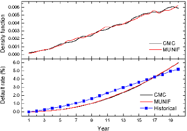
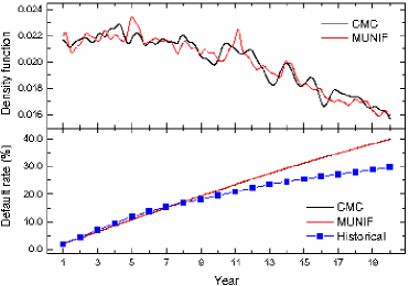
In this section, we demonstrate the developed model at work for analyzing the default events of two differently rated and correlated firms (denoted as A- and Ba-rated firms according to the Moody’s debt rating system) via a set of historical default data as presented by [8]. Our first task is to describe the first passage time density functions and default rates of these firms.
In order to apply our developed procedure, first we need to calibrate the developed model, in other words, to numerically choose or optimize the parameters, such as drift, volatility and jumps to fit the most liquid market data. As mentioned in Section 3, after Monte-Carlo simulation we obtain the estimated density by using the kernel estimator method. The cumulative default rates for firm in our model is defined as,
| (9) |
Then we minimize the difference between our model and historical default data to obtain the optimized parameters in the model (such as , arrival intensity in Eq. (4)):
| (10) |
For convenience, we reduce the number of optimizing parameters by:
-
1.
Setting and .
-
2.
Setting the growth rate of debt value equivalent to the growth rate of the firm’s value [8], so the default of firm is non-sensitive to . In our computations, we set .
-
3.
The interjump times satisfy an exponential distribution with mean value equals to 1.
-
4.
The arrival rate for jumps satisfies the Poisson distribution with intensity parameter , where the jump size is a normal distribution .
As a result, we only need to optimize , , , for each firm. This is done by minimizing the difference between our simulated default rates and historical data. Moreover, we assume there is only one driving Poisson shock with arrival rate . Hence we first optimize four parameters for, e.g., the A-rated firm, and then set the same for Ba-rated firm.
The minimization was performed by the using quasi-Newton procedure implemented as a Scilab program. The optimized parameters are described in Table 1.
| A | 0.0900 | 0.1000 | -0.2000 | 0.5000 |
|---|---|---|---|---|
| Ba | 0.1587 | 0.1000 | -0.5515 | 1.6412 |
By using these optimized parameters, we carried out the final simulation with Monte Carlo runs . Moreover, we also carried out simulations based on the conventional Monte-Carlo method with the same parameters and the discretization size of time horizon . The estimated first passage time density functions of A- and Ba-rated firms are shown in the top of Fig. 2 and 3, respectively. The simulated cumulative default rates (line) together with historical data (squares) are given in the bottom of Fig. 2 and 3. In Table 2, we give the calculated optimal bandwidths and the corresponding CPU times.
| CPU time | |||
|---|---|---|---|
| A | CMC | 0.892333 | 0.119668 |
| UNIF | 0.653902 | 0.000621 | |
| Ba | CMC | 0.427252 | 0.119675 |
| UNIF | 0.316703 | 0.000622 |
Based on these results, we conclude that:
-
1.
A-rated firm has a smaller Brownian motion part compared with Ba-rated firm, besides B-rated firm has large and especially large , which indicate that the loss due to sudden economic hazard may fluctuate a lot for Ba-rated firms.
-
2.
The density function of A-rated firm still has the trend to increase, which means the default rate of A-rated firm may increase little faster in future. As for Ba-rated firm, its density functions has decreased, so its default rate may increase very slowly or be kept at a constant level.
-
3.
From the CPU time in Table 2, we can conclude that the multivariate UNIF approach is much more efficient compared to the conventional Monte-Carlo method.
Our final example concerns with the default correlation of the two firms. We use the following conditions in our multivariate UNIF method:
-
1.
Setting and for all firms.
-
2.
Setting and for all firms.
- 3.
-
4.
The arrival rate for jumps satisfies the Poisson distribution with intensity parameter for both firms. The jump size is a normal distribution , where and can be different for different firms to reflect specifics of the jump process for each firm. We adopt the optimized parameters given in Table 1.
-
5.
As before, we generate the same interjump times that satisfy an exponential distribution with mean value equals to 1.
The simulated default correlations can be obtained via the following formula:
| (13) |
where is the probability of joint default for firms 1 and 2 in each Monte Carlo cycle, and are the cumulative default rates of firm 1 and 2, respectively, in each Monte Carlo cycle.
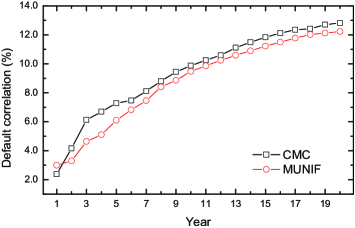
The simulated default correlations of A- and Ba-rate firms are given in Fig. 4. Based on these results, we can conclude that
-
1.
The default correlations tend to increase over long horizons and may converge to a stable value.
-
2.
Our developed methodology gives almost identical default correlations compared with the conventional Monte-Carlo method which confirms the validity of the developed methodology.
6 Conclusions
In this contribution, we developed efficient Monte-Carlo-based computational procedures for the solution of the FPT problem in the context of multivariate (and correlated) jump-diffusion processes. This was achieved by combining a fast Monte-Carlo method for one-dimensional jump-diffusion process and the generation of correlated multidimensional variables. The developed procedures were applied to the analysis of multivariate and correlated jump-diffusion processes. We have also discussed the implementation of the developed Monte-Carlo-based technique for multivariate jump-diffusion processes driving by several compound Poisson shocks. Finally, we have applied the developed technique to analyze the default events of two correlated firms via a set of historical default data. The developed methodology provides an efficient computational technique that is applicable in other areas of credit risk and pricing options.
7 Acknowledgements
This work was supported by NSERC.
References
- [1] S. Metwally and A. Atiya, Using Brownian bridge for fast simulation of jump-diffusion processes and barrier options, J. Derivatives, 10(2002), 43–54.
- [2] X. Zhang, Numerical analysis of American option pricing in a jump-diffusion model, Math. Oper. Res., 22(1997), 668–690.
- [3] C. Zhou, The Term Structure of Credit Spreads with Jump Risk, J. of Bank. Financ., 25(2001), 2015–2040.
- [4] A. F. Atiya and S. A. K. Metwally, Efficient Estimation of First Passage Time Density Function for Jump-Diffusion Processes, SIAM J. Sci. Comput., 26(2005), 1760–1775.
- [5] R. Cont and P. Tankov, Financial Modelling with Jump Processes, Chapman & Hall/CRC Press, London, 2003.
- [6] A. D. Crescenzo, E. D. Nardo and L. M. Ricciardi, Simulation of First-Passage Times for Alternating Brownian Motions, Methodol. Comput. Appl. Probab., 7(2005), 161–181.
- [7] F. Black and J. C. Cox, Valuing corporate securities: Some effects of bond indenture provisions, J. Financ., 31(1976), 351–367.
- [8] C. Zhou, An analysis of default correlation and multiple defaults, Rev. Finan. Stud., 14(2001), 555–576.
- [9] J. Hull and A. White, Valuing Credit Default Swaps II: Modeling Default Correlations, J. Derivatives, 8(2001), 12–22.
- [10] B. W. Silverman, Density Estimation for Statistics and Data Analysis, Chapman and Hall, New York, 1986.
- [11] P. Glasserman, Monte Carlo Methods in Financial Engineering, Springer, New York, 2004.
- [12] P. E. Kloeden, E. Platen and H. Schurz, Numerical Solution of SDE Through Computer Experiments, Springer, Germany, 2003.
- [13] J. T. Chen, Using the sum-of-uniforms method to generate correlated random variates with certain marginal distribution, Eur. J. Oper. Res., 167(2005), 226–242.
- [14] D. Zhang and R. V. N. Melnik, Efficient estimation of default correlation for multivariate jump-diffusion processes, Financ. Stoch., submitted.
- [15] D. Zhang and R. V. N. Melnik, Monte-Carlo Simulations of the First Passage Time for Multivariate Jump-Diffusion Processes in Financial Applications, Quant. Financ., submitted.