Efficient estimation of default correlation for multivariate jump-diffusion processes

Abstract

Evaluation of default correlation is an important task in credit risk analysis. In many practical situations, it concerns the joint defaults of several correlated firms, the task that is reducible to a first passage time (FPT) problem. This task represents a great challenge for jump-diffusion processes (JDP), where except for very basic cases, there are no analytical solutions for such problems. In this contribution, we generalize our previous fast Monte-Carlo method (non-correlated jump-diffusion cases) for multivariate (and correlated) jump-diffusion processes. This generalization allows us, among other things, to evaluate the default events of several correlated assets based on a set of empirical data. The developed technique is an efficient tool for a number of other applications, including credit risk and option pricing.

Keywords: Default correlation, First passage time problem, Monte Carlo simulation

JEL classification: C15

Mathematics Subject Classification (2000): 65C05, 60J10, 60J75

1 Introduction

In the financial world, individual companies are usually linked together via economic conditions, so default correlation, defined as the risk of multiple companies’ default together, has been an important area of research in credit analysis with applications to joint default, credit derivatives, asset pricing and risk management.

Nevertheless, the development of efficient computational tools for modeling default correlation is lagging behind its practical needs. Currently, there are two dominant groups of theoretical models used in default correlation. One is a reduced form model, such as in [12] that uses a Copula function to parameterize the default correlation. Recently, Chen et al [4] have translated the joint default probability into bivariate normal probability function.

The second group of models for default correlation is a structural form model. Zhou [16] and Hull et al [8] are the first to incorporate default correlation into the Black-Cox first passage structural model. They got similar closed form solutions for two assets. However, their models cannot easily be extended to more than two assets. Furthermore, the developed models do not include jump-diffusion processes.

As demonstrated in [17], jump risk becomes an important factor in credit risk analysis. It is now widely acknowledged that the standard Brownian motion model for market behavior falls short of explaining empirical observations of market returns and their underlying derivative prices [11]. The (multivariate) jump-diffusion model that provides a convenient framework for investigating default correlation with jumps becomes more readily accepted in the financial world.

One of the major problems in default analysis is to determine when a default will occur within a given time horizon, or in other words, what the default rate is during such a time horizon. This problem is reduced to a first passage time (FPT) problem that can be formalized on a basis of a certain stochastic differential equations (SDE). It concerns the estimation of the probability density of the time for a random process to cross a specified threshold level. Unfortunately, after including jumps, only special cases have analytical solutions. For most practical cases, closed form solutions are unavailable and we can only turn to the numerical procedures.

Monte Carlo simulation is such a candidate for solving the SDE, arising in the context of FPT problem. In conventional Monte Carlo methods, we need to discretize the time horizon into small enough intervals in order to avoid discretization bias [10], and we need to evaluate the processes at each discretized time which is very time-consuming. Many researchers have contributed to the field and enhanced the efficiency of Monte Carlo simulation. Atiya and Metwally [1, 13] have developed a fast Monte Carlo-type numerical method to solve the FPT problem. Recently, we have reported an extension of this fast Monte Carlo-type method in the context of multiple non-correlated jump-diffusion processes [15].

In this contribution, we develop a methodology for solving the FPT problem in the context of multivariate jump-diffusion processes. In particular, we have generalized the reported fast Monte-Carlo method (non-correlated jump-diffusion cases) for multivariate (and correlated) jump-diffusion processes. The paper is organized in the following way: Section 2 details the description of our model. The algorithms are described in Section 3. Section 4 contains the simulation results and discussions, followed by the conclusions given in Section 5.

2 Developing multi-dimensional model

2.1 Default correlation

In the market economy, individual companies are inevitably linked together via dynamically changing economic conditions. Take two firms A and B as an example, whose probabilities of default are $P_{A}$ and $P_{B}$, respectively. Then the default correlation can be defined as

$$\rho_{AB}=\frac{P_{AB}-P_{A}P_{B}}{\sqrt{P_{A}(1-P_{A})P_{B}(1-P_{B})}},$$ (1)

where $P_{AB}$ is the probability of joint default.

Now, we can write $P_{AB}$ as $P_{AB}=P_{A}P_{B}+\rho_{AB}\sqrt{P_{A}(1-P_{A})P_{B}(1-P_{B})}$. If we assume $P_{A}=P_{B}=p\ll 1$, then we have $P_{AB}\approx p^{2}+\rho_{AB}p\approx\rho_{AB}p$. Thus it is apparent that the default correlation $\rho_{AB}$ plays a key role in the joint default with important implication in the field of credit analysis. Zhou [16] and Hull et al [8] were the first to incorporate default correlation into the Black-Cox first passage structural model.

In [16] Zhou has proposed a first passage time model to describe default correlations of two firms under the “bivariate diffusion process”:

$$\left[\begin{array}[]{cc}d\ln(V_{1})\\ d\ln(V_{2})\end{array}\right]=\left[\begin{array}[]{cc}\mu_{1}\\ \mu_{2}\end{array}\right]dt+\Omega\left[\begin{array}[]{cc}dz_{1}\\ dz_{2}\end{array}\right],$$ (2)

where $\mu_{1}$ and $\mu_{2}$ are constant drift terms, $z_{1}$ and $z_{2}$ are two independent standard Brownian motions, and $\Omega$ is a constant $2\times 2$ matrix such that

$$\Omega\cdot\Omega^{\prime}=\left[\begin{array}[]{cc}\sigma_{1}^{2}&\rho\sigma_{1}\sigma_{2}\\ \rho\sigma_{1}\sigma_{2}&\sigma_{2}^{2}\end{array}\right].$$

The coefficient $\rho$ reflects the correlation between the movements in the asset values of the two firms. Based on Eq. (2), Zhou has deduced the closed form solution of default correlations of two assets [16]. However, none of the above models has included possible jumps. Apparently, jumps have more significant importance in the default correlation than often perceived. Indeed, simultaneous jumps may enhance the chance of simultaneous defaults which increases the correlation defaults.

2.2 Multivariate jump-diffusion process

Let us consider a more general case. In a complete probability space $(\Omega,F,P)$ with information filtration $(F_{t})$. Suppose that $X_{t}=\ln(V_{t})$ is a Markov process in some state space $D\subset\mathbb{R}^{n}$, solving the stochastic differential equation [7]

$$dX_{t}=\mu(X_{t})dt+\sigma(X_{t})dW_{t}+dZ_{t},$$ (3)

where $W$ is an $(F_{t})$-standard Brownian motion in $\mathbb{R}^{n}$; $\mu:D\rightarrow\mathbb{R}^{n}$, $\sigma:D\rightarrow\mathbb{R}^{n\times n}$, and $Z$ is a pure jump process whose jumps have a fixed probability distribution $\nu$ on $\mathbb{R}^{n}$ such that they arrive with intensity $\{\lambda(X_{t}):t\geq 0\}$, for some $\lambda:D\rightarrow[0,\infty)$. Under these conditions, the above model is reduced to an affine model if [7]:

$$\mu(X_{t},t)=K_{0}+K_{1}X_{t}$$

$$(\sigma(X_{t},t)\sigma(X_{t},t)^{\top})_{ij}=(H_{0})_{ij}+(H_{1})_{ij}X_{j}$$

$$\lambda(X_{t})=l_{0}+l_{1}\cdot X_{t},$$ (4)

where $K=(K_{0},K_{1})\in\mathbb{R}^{n}\times\mathbb{R}^{n\times n}$, $H=(H_{0},H_{1})\in\mathbb{R}^{n\times n}\times\mathbb{R}^{n\times n\times n}$, $l=(l_{0},l_{1})\in\mathbb{R}^{n}\times\mathbb{R}^{n\times n}$.

If we assume that,

1. Each $W_{t}$ in Eq. (3) is independent;

2. $K_{1}=0$, $H_{1}=0$ and $l_{1}=0$ in (4) that means the drift term, the diffusion process (Brownian motion) and the arrival intensity are independent with state vector $X_{t}$;

3. The distribution of jump-size $Z_{t}$ is also independent with respect to $X_{t}$.

In this scenario, we can rewrite Eq. (3) as

$$dX_{t}=\mu dt+\sigma dW_{t}+dZ_{t},$$ (5)

where

$$\mu=K_{0},\;\sigma\sigma^{\top}=H_{0},\;\lambda=l_{0}.$$

At first sight, Eq. (5) is similar to Eq. (2), but Eq. (5) is a much more general model that can be applied to multiple firms, and where jumps have been taken into account.

2.3 First passage time distribution

Let us consider a firm $i$, as described by Eq. (5), such that its state vector $X_{i}$ satisfies the following SDE:

$$dX_{i}=\mu_{i}dt+\sum_{j}\sigma_{ij}dW_{j}+dZ_{i}=\mu_{i}dt+\sigma_{i}dW_{i}+dZ_{i},$$ (6)

where $W_{i}$ is a standard Brownian motion and $\sigma_{i}$ is:

$$\sigma_{i}=\sqrt{\sum_{j}\sigma_{ij}^{2}}.$$

We assume that in the interval $[0,T]$, total number of jumps for firm i is $M_{i}$ times of jumps. Let the jump instants be $T_{1},T_{2},\cdots,T_{M_{i}}$. Let $T_{0}=0$ and $T_{M_{i}+1}=T$. The quantities $\tau_{j}$ equal to interjump times, which is $T_{j}-T_{j-1}$. Let $X_{i}(T_{j}^{-})$ be the process value immediately before the $j$th jump, and $X_{i}(T_{j}^{+})$ be the process value immediately after the $j$th jump. The jump-size is $X_{i}(T_{j}^{+})-X_{i}(T_{j}^{-})$, we can use such jump-sizes to generate $X_{i}(T_{j}^{+})$ sequentially.

In a structural model, a firm defaults when the firm assets value $V_{t}$ falls below a threshold level $D_{V}(t)$. In this contribution, we use an exponential form, defining the threshold level by $D_{V}(t)=\kappa\exp(\gamma t)$ as proposed in [16], where $\gamma$ can be interpreted as the growth rate of firm’s liabilities. Coefficient $\kappa$, in front, captures the liability structure of the firm, which is usually defined as a firm’s short-term liability plus 50% of the firm’s long-term liability. As mentioned before, $X_{t}=\ln(V_{t})$, then the threshold of $X_{t}$ is $D(t)=\gamma t+\ln(\kappa)$.

Atiya et al [1] have deduced a one-dimensional first passage time distribution in time horizon $[0,T]$. In order to evaluate multi-firms, we obtain multi-dimensional formulas and reduce them to computable forms.

First, let us define $A_{i}(t)$ as the event that process crossed the threshold level $D_{i}(t)$ for the first time in the interval $[t,t+dt]$. Then we have

$$g_{ij}(t)=p(A_{i}(t)\in dt|X_{i}(T_{j-1}^{+}),X_{i}(T_{j}^{-})).$$ (7)

If we only consider one interval $[T_{j-1},T_{j}]$, we can obtain

$$g_{ij}(t) = \frac{X_{i}(T_{j-1}^{+})-D_{i}(t)}{2y_{i}\pi\sigma_{i}^{2}}(t-T_{j-1})^{-\frac{3}{2}}(T_{j}-t)^{-\frac{1}{2}}$$ (8)

$$*\exp\left(-\frac{[X_{i}(T_{j}^{-})-D_{i}(t)-\mu_{i}(T_{j}-t)]^{2}}{2(T_{j}-t)\sigma_{i}^{2}}\right)$$

$$*\exp\left(-\frac{[X_{i}(T_{j-1}^{+})-D_{i}(t)+\mu_{i}(t-T_{j-1})]^{2}}{2(t-T_{j-1})\sigma_{i}^{2}}\right),$$

where

$$y_{i}=\frac{1}{\sigma_{i}\sqrt{2\pi\tau_{j}}}\exp\left(-\frac{[X_{i}(T_{j-1}^{+})-X_{i}(T_{j}^{-})+\mu_{i}\tau_{j}]^{2}}{2\tau_{j}\sigma_{i}^{2}}\right).$$

After getting these results in one interval, we combine the results to obtain the density for the whole interval $[0,T]$. Let $B(s)$ be a Brownian bridge in the interval $[T_{j-1},T_{j}]$ with $B(T_{j-1}^{+})=X_{i}(T_{j-1}^{+})$ and $B(T_{j}^{-})=X_{i}(T_{j}^{-})$. Then the probability that the minimum of $B(s_{i})$ is always above the boundary level is

$$P_{ij} = P\left(\inf_{T_{j-1}\leq s_{i}\leq T_{j}}B(s_{i})>D_{i}(t)|B(T_{j-1}^{+})=X_{i}(T_{j-1}^{+}),B(T_{j}^{-})=X_{i}(T_{j}^{-})\right)$$ (11)

$$= \left\{\begin{array}[]{ll}1-\exp\left(-\frac{2[X_{i}(T_{j-1}^{+})-D_{i}(t)][X_{i}(T_{j}^{-})-D_{i}(t)]}{\tau_{j}\sigma_{i}^{2}}\right),&\mathrm{if}\;X_{i}(T_{j}^{-})>D_{i}(t),\\ 0,&\mathrm{otherwise}.\end{array}\right.$$

This implies that $B(s_{i})$ is below the threshold level, which means the default happens or already happened, and its probability is $1-P_{ij}$. Let $L(s_{i})\equiv L_{i}$ denote the index of the interjump period in which the time $s_{i}$ falls in $[T_{L_{i}-1},T_{L_{i}}]$. Also, let $I_{i}$ represent the index of the first jump, which happened in the simulated jump instant:

$$I_{i} = \min(j:X_{i}(T_{k}^{-})>D_{i}(t);k=1,\ldots,j,\;\mathrm{and}$$ (12)

$$\;\;\;\;\;\;\;\;\;\;\;\>X_{i}(T_{k}^{+})>D_{i}(t);k=1,\ldots,j-1,\;\mathrm{and}\;X_{i}(T_{j}^{+})\leq D_{i}(t)).$$

If no such $I_{i}$ exists, then we set $I_{i}=0$.

By combining Eq. (8), (11) and (12), we get the probability of $X_{i}$ crossing the boundary level in the whole interval $[0,T]$ is

$$P(A_{i}(s_{i})\in ds|X_{i}(T_{j-1}^{+}),X_{i}(T_{j}^{-}),j=1,\ldots,M_{i}+1)$$ (16)

$$= \left\{\begin{array}[]{ll}g_{iL_{i}}(s_{i})\prod_{k=1}^{L_{i}-1}P_{ik}&\mathrm{if}\;L_{i}<I_{i}\;\mathrm{or}\;I_{i}=0,\\ g_{iL_{i}}(s_{i})\prod_{k=1}^{L_{i}-1}P_{ik}+\prod_{k=1}^{L_{i}}P_{ik}\delta(s_{i}-T_{I_{i}})&\mathrm{if}\;L_{i}=I_{i},\\ 0&\mathrm{if}\;L_{i}>I_{i},\end{array}\right.$$

where $\delta$ is the Dirac’s delta function.

2.4 The kernel estimator

For each firm, after generating a series of first passage times $s_{i}$, we use a kernel density estimator with Gaussian kernel to estimate the first passage time density (FPTD) $f$. As described in [1], the kernel density estimator is based on centering a kernel function of a bandwidth as follows:

$$\widehat{f}=\frac{1}{N}\sum_{i=1}^{N}K(h,t-s_{i}),$$ (17)

where

$$K(h,t-s_{i})=\frac{1}{\sqrt{\pi/2}h}\exp\left(-\frac{(t-s_{i})^{2}}{h^{2}/2}\right).$$

The optimal bandwidth in the kernel function $K$ can be calculated as [14]:

$$h_{opt}=\left(2N\sqrt{\pi}\int_{-\infty}^{\infty}(f_{t}^{\prime\prime})^{2}dt\right)^{-0.2},$$ (18)

where $N$ is the number of generated points and $f_{t}$ is the true density. Here we use the approximation for the distribution, as a gamma distribution as proposed in [1]:

$$f_{t}=\frac{\alpha^{\beta}}{\Gamma(\beta)}t^{\beta-1}\exp(-\alpha t).$$ (19)

So the integral in Eq. (18) becomes,

$$\int_{0}^{\infty}(f_{t}^{\prime\prime})^{2}dt=\sum_{i=1}^{5}\frac{W_{i}\alpha_{i}\Gamma(2\beta-i)}{2^{(2\beta-i)}(\Gamma(\beta))^{2}},$$ (20)

where

$$W_{1}=A^{2},\;\;W_{2}=2AB,\;\;W_{3}=B^{2}+2AC,\;\;W_{4}=2BC,\;\;W_{5}=C^{2},$$

and

$$A=\alpha^{2},\;\;B=-2\alpha(\beta-1),\;\;C=(\beta-1)(\beta-2).$$

From Eq. (20), follows that in order to get a nonzero bandwidth, we have constraint $\beta$ to be at least equal to 3.

After obtaining the estimated first passage time density $\widehat{f}$, the cumulative default rates can be written as,

$$P_{i}(t)=\int_{0}^{t}\widehat{f}_{i}(\tau)d\tau.$$ (21)

3 Methodology of the solution

In Section 2, we have reduced the solution of the original problem to a multivariate jump-diffusion model as described in Eq. (6). The first passage time distribution was obtained in Section 2.3. As we have already noted, once jumps are included in the process, only for very basic applications closed form solutions are available [11, 2], which in most practically interesting cases we have to resort to the numerical procedures.

Let us recall the conventional Monte-Carlo procedure in application to the analysis of the evaluation of firm $X_{i}$ within the time horizon $[0,T]$. We divide the time horizon into $n$ small intervals $[0,t_{1}]$, $[t_{1},t_{2}]$, $\cdots$, $[t_{n-1},T]$ as displayed in Fig. 1(a). In each Monte Carlo run, we need to calculate the value of $X_{i}$ at each discretized time $t$. As usual in order to exclude discretization bias, the number $n$ must be large. This procedure exhibits substantial computational difficulties when applied to jump-diffusion process.

Indeed, for a typical jump-diffusion process, as shown in Fig. 1(a), let $T_{j-1}$ and $T_{j}$ be any successive jump instants, as described above. Then, in the conventional Monte Carlo method, although there is no jump occurring in the interval $[T_{j-1},T_{j}]$, yet we need to evaluate $X_{i}$ at each discretized time $t$ in $[T_{j-1},T_{j}]$. This very time-consuming procedure results in serious shortcoming of the conventional Monte Carlo methodology.

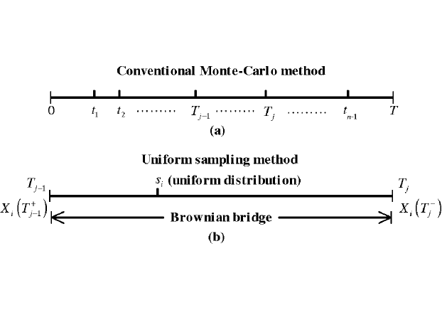
Figure 1: Schematic diagram of (a) conventional Monte Carlo and (b) uniform sampling method.

To remedy the situation, two modifications of the conventional procedure were recently proposed by Atiya and Metwally [1, 13] that allow us a potential speed-up of the conventional methodology in 10-30 times. One of the modifications, the uniform sampling method, involves sampling method. The other, inverse Gaussian density sampling, is based on the inverse Gaussian density method for sampling. Both methodologies were developed for the univariate case.

In this article, we focus on the further development of uniform sampling (UNIF) method and extend it to multivariate jump-diffusion processes. The major improvement of the uniform sampling method is based on the fact that it only evaluates $X_{i}$ at generated jump instants while between each two jumps the process is a Brownian bridge (see Fig. 1(b)). Hence we just consider the probability of $X_{i}$ defaults in $(T_{j-1},T_{j})$ instead of evaluating $X_{i}$ at each discretized time $t$. More precisely, in the uniform sampling method, we assume that the values of $X_{i}(T_{j-1}^{+})$ and $X_{i}(T_{j}^{-})$ are known as two end points of the Brownian bridge, we generate a variable $s_{i}$ with uniform distribution and by using Eq. (11) we verify whether $X_{i}(s_{i})$ is smaller than the threshold level. If it is, then we have successfully generated a first passage time $s_{i}$ and can neglect the other intervals and perform another Monte Carlo run.

In order to implement the UNIF method for our multivariate model as described in Eq. (6), we need to consider several points as follows:

1. Here, we focus on the firms rated in the same way, that is we assume that the arrival rate $\lambda$ for the Poisson jump process and the distribution of $(T_{j}-T_{j-1})$ are the same for each firm. As for the jump-size, we generate them by a given distribution, which can be different for different firms to reflect specifics of the jump process for each firm.

2. We exemplify our description by considering an exponential distribution (mean value $\mu_{T}$) for $(T_{j}-T_{j-1})$ and a normal distribution (mean value $\mu_{J}$ and standard deviation $\sigma_{J}$) for the jump-size. We can use any other distribution when appropriate.

3. An array IsDefault (whose size is the number of firms denoted by $N_{\mathrm{firm}}$) was used to indicate whether firm $i$ has defaulted in this Monte Carlo run. If the firm defaults, then we set IsDefault$(i)=1$, and will not evaluate it during this Monte Carlo run.

4. Most importantly, in order to reflect the correlations of multiple firms, we need to generate correlated $s_{i}$. As deduced in [9, 16], the joint probability of firm $i$ to default before $s_{i}$ and firm $j$ to default before $s_{j}$ satisfies the bivariate inverse Gaussian distribution. We approximate the correlation between $s_{i}$ and $s_{j}$, denoted further by $\rho_{s_{i},s_{j}}$ as the default correlation of firm $i$ and $j$. Then, we employ the sum-of-uniforms method [3] to generate correlated uniform numbers $s_{i}$.

Our algorithm for multivariate jump-diffusion processes can be described as follows. It is an extension of the one-dimensional case, described in [1, 13].

Consider $N_{\mathrm{firm}}$ firms in the interval $[0,T]$. First, we generate the jump instant $T_{j}$ by generating interjump times $(T_{j}-T_{j-1})$, and set all the IsDefault$(i)=0$ to indicate that no firm defaults at first.

From Fig. 1(b) and Eq. (6), we can conclude that,

1. If no jump occurs, as described in Eq. (6), the interjump size $(X_{i}(T_{j}^{-})-X_{i}(T_{j-1}^{+}))$ follows a normal distribution of mean $\mu_{i}(T_{j}-T_{j-1})$ and standard deviation $\sigma_{i}\sqrt{T_{j}-T_{j-1}}$. We get

   $$X_{i}(T_{j}^{-}) \sim X_{i}(T_{j-1}^{+})+\mu_{i}(T_{j}-T_{j-1})+\sigma_{i}N(0,T_{j}-T_{j-1})$$

   $$\sim X_{i}(T_{j-1}^{+})+\mu_{i}(T_{j}-T_{j-1})+\sum_{k=1}^{N_{\mathrm{firm}}}\sigma_{ik}N(0,T_{j}-T_{j-1}),$$

   where the initial state is $X_{i}(0)=X_{i}(T_{0}^{+})$.

2. If jump occurs, we simulate the jump-size by a normal distribution or other distribution when appropriate, and compute the postjump value:

   $$X_{i}(T_{j}^{+})=X_{i}(T_{j}^{-})+Z_{i}(T_{j}).$$

After generating beforejump and postjump values $X_{i}(T_{j}^{-})$ and $X_{i}(T_{j}^{+})$. As before, $j=1,...,M$ where $M$ is the number of jumps for all the firms, we can compute $P_{ij}$ according to Eq. (11). To recur the first passage time density (FPTD) $f_{i}(t)$, we have to consider three possible cases that may occur for each non-default firm $i$:

1. First passage happens inside the interval. We know if $X_{i}(T_{j-1}^{+})>D_{i}(T_{j-1})$ and $X_{i}(T_{j}^{-})<D_{i}(T_{j})$, then the first passage happened in the time interval $[T_{j-1},T_{j}]$. To evaluate when the first passage happened, we introduce a new viable $b_{ij}$, as $b_{ij}=\frac{T_{j}-T_{j-1}}{1-P_{ij}}$, so that $T_{j-1}+b_{ij}=\frac{T_{j}-P_{ij}T_{j-1}}{1-P_{ij}}$. By using the sum-of-uniforms method, we generate several correlated uniform numbers $s_{i}$ in the interval of $[T_{j-1},T_{j-1}+b_{ij}]$, and if $s_{i}$ also belongs to interval $[T_{j-1},T_{j}]$, then the first passage time occurred in this interval. We set IsDefault$(i)=1$ to indicate firm $i$ that has defaulted. Then, we can compute the conditional boundary crossing density $g_{ij}(s_{i})$ according to Eq. (8). To get the density of the entire interval $[0,T]$, we use $\widehat{f}_{i,n}(t)=\left(\frac{T_{j}-T_{j-1}}{1-P_{ij}}\right)g_{ij}(s_{i})*K(h_{opt},t-s_{i})$, where $n$ is the iteration number of the Monte Carlo cycle.

2. First passage does not happen in the current interval. If $s_{i}$ doesn’t belong to interval $[T_{j-1},T_{j}]$, then the first passage time has not yet occurred in this interval.

3. First passage happens at the right boundary of interval. If $X_{i}(T_{j}^{+})<D_{i}(T_{j})$ and $X_{i}(T_{j}^{-})>D_{i}(T_{j})$ (see Eq. (12)), then $T_{I_{i}}$ is the first passage time and $I_{i}=j$. We evaluate the density function using kernel function $\widehat{f}_{i,n}(t)=K(h_{opt},t-T_{I_{i}})$, and set IsDefault$(i)=1$.

Next, we increase $j$ and examine the next interval and analyze the above three cases for each non-default firm again. After running $N$ times the Monte Carlo cycle, we get the FPTD of firm $i$ as $\widehat{f}_{i}(t)=\frac{1}{N}\sum_{n=1}^{N}\widehat{f}_{i,n}(t)$, as well as the cumulative default rates $P_{i}(t)=\int_{0}^{t}\widehat{f}_{i}(\tau)d\tau$.

4 Applications and discussion

In this section, we will demonstrate how our model describes the default correlations of the firms, rated in the same way, via studying the historical data. We provide details on the calibration of the models we apply for this description.

4.1 Default rates

In Fig. 2, the black line of square is a set of historical default data of A-rated firm taken from [16].

First, if we do not consider jumps, as assumed in [16], the firm defaults at time $t$ with probability:

$$P_{i}(t)=2\cdot N\left(-\frac{X_{i}(0)-\ln(\kappa_{i})}{\sigma_{i}\sqrt{t}}\right)=2\cdot N\left(-\frac{Z_{i}}{\sqrt{t}}\right),$$ (22)

where

$$Z_{i}\equiv\frac{X_{i}(0)-\ln(\kappa_{i})}{\sigma_{i}}$$

is the standardized distance of firm $i$ to its default point and $N(\cdot)$ denotes the cumulative probability distribution function for a standard normal variable.

If historical default rates are given, we can estimate $Z_{i}$ as follows:

$$Z_{i}=\mathrm{arg}\min_{Z_{i}}\sum_{t}\left(\frac{P_{i}(Z_{i},t)}{t}-\frac{\widetilde{A}_{i}(t)}{t}\right)^{2},$$ (23)

where $P_{i}(Z_{i},t)$ are the theoretical default probabilities (as determined by Eq. (22)) and $\widetilde{A}_{i}(t)$ are the historical default rates. For the A-rated firm considered here, the optimized $Z_{i}$ value was evaluated in [16] as $8.06$. By feeding the optimized $Z_{i}$-value into Eq. (22), we get the theoretical cumulative default rates without jumps, given in Fig. 2 by the line of circles.

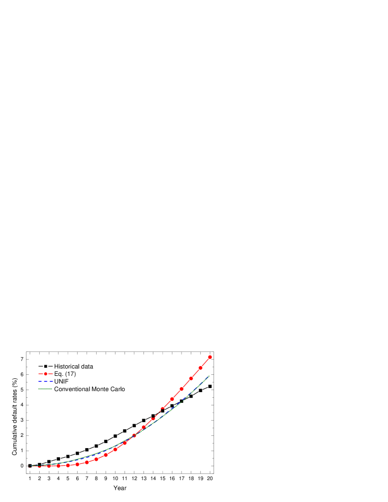
Figure 2: Historical, theoretical and simulated cumulative default rates. The theoretical value is calculated by using Eq. (22). All the simulations were performed with Monte Carlo runs $N=100,000$, besides, for conventional Monte Carlo method, the discretization size of time horizon is $\Delta=0.005$.

Now, let us consider the UNIF method, developed in Section 2.4 and 3. First, the developed Monte Carlo simulation allows us to obtain the estimated density $\widehat{f}_{i}(t)$ by using kernel estimator method. We get also the default rate $P_{i}(t)$ for firm $i$.

Then we minimize the difference between our model and the historical default data to obtain the optimized parameters in our model:

$$\mathrm{argmin}\left(\sum_{i}\sqrt{\sum_{t_{j}}\left(\frac{P_{i}(t_{j})-\widetilde{A}_{i}(t_{j})}{t_{j}}\right)^{2}}\right).$$ (24)

For convenience, we reduce the number of optimizing parameters by:

1. Setting $X(0)=2$ and $\ln(\kappa)=0$.

2. Setting the growth rate $\gamma$ of debt value equivalent to the growth rate $\mu$ of the firm’s value [16], so the default of firm is non-sensitive to $\mu$. Setting $\mu=-0.001$ in our computation reported next.

3. The interjump times $(T_{j}-T_{j-1})$ satisfy an exponential distribution with mean value equals to 1.

4. The arrival rate for jumps satisfies the Poisson distribution with intensity parameter $\lambda$, where the jump size is a normal distribution $Z_{t}\sim N(\mu_{Z},\sigma_{Z})$.

As a result, we only need to optimize $\sigma$, $\lambda$, $\mu_{Z}$, $\sigma_{Z}$ for this firm, This is done by minimizing the differences between our simulated default rates and the given historical data. The minimization was performed by using quasi-Newton procedure implemented as a Scilab program.

The optimized parameters for the A-rated firm are $\sigma=0.09000984$, $\lambda=0.10001559$, $\mu_{Z}=-0.20003641$, and $\sigma_{Z}=0.50000485$. Then, by using these optimized parameters, we carried out a final simulation with Monte Carlo runs $N=100,000$. The simulated cumulative default rates by using the UNIF method are shown in Fig. 2 by the dash line. For comparison, we have carried out the conventional Monte Carlo simulation with the same optimized parameters. The resulting simulated default rates are displayed by dotted line in Fig. 2. All the simulations reported here were carried out on a 2.4 GHz AMD Opteron(tm) Processor. The optimal bandwidth and CPU time are given in Table 1.

Table 1: The optimal bandwidth $h_{opt}$, and CPU time per Monte Carlo run of the simulations. All the simulations were performed with Monte Carlo runs $N=100,000$; the discretization size of time horizon for the conventional Monte Carlo method was $\Delta=0.005$.

	Optimal bandwidth	CPU time per Monte Carlo run
Conventional Monte Carlo	0.891077	0.119668
UNIF	0.655522	0.000621

From Fig. 2, we can conclude that our simulations give similar results to the theoretically predicted by Eq. (22), and exceed them for short time horizon. The UNIF method gives exactly the same default curve as the conventional Monte Carlo method, but the former outperforms the latter substantially in terms of computational time. The UNIF methodology is much faster compared to the conventional method and is extremely useful in practical application.

4.2 Default correlations

Our final example concerns with the default correlation of two A-rated firms (A,A). In Table 2 we provide the information on the default correlation of firms (A,A) for one-, two-, five- and ten-year. The values in the 2nd column were calculated by using the closed form solution derived in [16].

Table 2: Theoretical and simulated default correlations (%) of firms (A,A). The simulations were performed with Monte Carlo runs $N=100,000$.

Year	Ref. [16]	UNIF
1	0.00	0.00
2	0.02	2.47
5	1.65	6.58
10	7.75	9.28

In order to implement the UNIF method, we use assumptions, similar to the ones before, in order to reduce the number of optimized parameters:

1. Setting $X(0)=2$ and $\ln(\kappa)=0$ for all firms.

2. Setting $\gamma=\mu$ and $\mu=-0.001$ for all firms.

3. Since we are considering two same rated firms (A,A), we choose $\sigma$ as:

   $$\sigma=\left[\begin{tabular}[]{cc}$\sigma_{11}$&$\sigma_{12}$\\ $\sigma_{21}$&$\sigma_{22}$\end{tabular}\right],$$ (25)

   where $\sigma\sigma^{\top}=H_{0}$ such that

   $$\sigma\sigma^{\top}=H_{0}=\left[\begin{tabular}[]{cc}$\sigma_{1}^{2}$&$\rho_{12}\sigma_{1}\sigma_{2}$\\ $\rho_{12}\sigma_{1}\sigma_{2}$&$\sigma_{2}^{2}$\end{tabular}\right],$$ (26)

   and

   $$\left\{\begin{tabular}[]{l}$\sigma_{1}^{2}=\sigma_{11}^{2}+\sigma_{12}^{2}$\\ $\sigma_{2}^{2}=\sigma_{21}^{2}+\sigma_{22}^{2}$\\ $\rho_{12}=\displaystyle\frac{\sigma_{11}\sigma_{21}+\sigma_{12}\sigma_{22}}{\sigma_{1}\sigma_{2}}$\end{tabular}\right.,$$ (27)

   In (27), $\rho_{12}$ reflects the correlation of diffusion parts of the state vectors of the two firms.

4. The arrival rate for jumps satisfies the Poisson distribution with intensity parameter $\lambda$ for all firms, and we use the parameters optimized based on a single A-rated firm, i.e., $\lambda=0.10001559$ for all the firms.

5. As before, we generate the same interjump times $(T_{j}-T_{j-1})$ that satisfies an exponential distribution with mean value equals 1 for all firms. Furthermore, the jump size is a normal distribution $Z_{t}\sim N(\mu_{Z_{i}},\sigma_{Z_{i}})$, and we use the parameters optimized from a single A-rated firm, i.e., $\mu_{Z_{i}}=-0.20003641$ and $\sigma_{Z_{i}}=0.50000485$ for all the firms.

As a result, there are only 4 parameters left to optimize: $\sigma_{11}$, $\sigma_{12}$, $\sigma_{21}$ and $\sigma_{22}$. The optimization was carried out by using the quasi-Newton procedure implemented as a Scilab program. The resulting optimized parameters are $\sigma_{11}=0.06963755$, $\sigma_{12}=0.02993134$, $\sigma_{21}=0.03387809$ and $\sigma_{22}=0.06691001$. We can easily get $\sigma_{1}=0.0757976$, $\sigma_{2}=0.0749978$ and $\rho_{12}=0.7673104$. The parameter $\rho_{12}$ represents the correlation between diffusion parts of the state vectors of two firms.

The simulated default correlations are displayed in the 3rd column of Table 2. Observe that, the UNIF method gives a little larger default correlation compared to the theoretical predicted by Eq. (22). This is mainly because our optimized $\rho_{12}$ is larger than $0.4$ used in [16], and we have used the same interjump times $(T_{j}-T_{j-1})$ for all the firms. Nevertheless, the UNIF method gives the correct default correlation trend, as the default correlation becomes larger with increasing time.

5 Conclusion

We analyzed the first passage time problem in the context of multivariate and correlated jump-diffusion processes by extending the fast Monte Carlo-type numerical method – the UNIF method – to the multivariate case. We provided an application example of simulating default correlations confirming the validity of our model and the developed algorithm. Finally, we note that the developed methodology provides an efficient tool for further practical applications such as in credit analysis and barrier option pricing.

References

- [1] Atiya, A.F., Metwally, S.A.K.: Efficient Estimation of First Passage Time Density Function for Jump-Diffusion Processes. SIAM Journal on Scientific Computing 26, 1760–1775 (2005)
- [2] Blake, I., Lindsey, W.: Level-crossing problems for random processes. IEEE Trans. Inform. Theory 19, 295–315 (1973)
- [3] Chen J.T.: Using the sum-of-uniforms method to generate correlated random variates with certain marginal distribution. European Journal of Operational Research 167, 226–242 (2005)
- [4] Chen, R.R., Sopranzetti, B.J.: The Valuation of Default-Triggered Credit Derivatives. Journal of Financial and Quantitative Analysis 38, 359–382 (2003)
- [5] Costa, O., Fragoso, M.: Discrete time LQ-optimal control problems for infinite Markov jump parameter systems. IEEE Trans. Automat. Control 40, 2076–2088 (1995)
- [6] Devroye, L.: Non-uniform Random Variate Generation. Springer-Verlag: New York 1986
- [7] Duffie, D., Pan, J., Singleton, K.: Transform Analysis and Option Pricing for Affine Jump-Diffusions. Econometrica 68, 1343–1376 (2000)
- [8] Hull, J., White, A.: Valuing Credit Default Swaps II: Modeling Default Correlations. Journal of Derivatives 8, 12–22 (2001)
- [9] Iyengar, S.: Hitting lines with two-dimensional Brownian motion. SIAM Journal of Applied Mathematics 45, 983–989 (1985)
- [10] Kloeden, P.E., Platen, E., Schurz, H.: Numerical Solution of SDE Through Computer Experiments, Third Revised Edition. Springer: Germany 2003
- [11] Kou, S.G., Wang, H.: First passage times of a jump diffusion process. Adv. Appl. Probab. 35, 504–531 (2003)
- [12] Li, D.X.: On Default Correlation: A Copula Approach. Journal of Fixed Income 9, 43–54 (2000)
- [13] Metwally, S., Atiya, A.: Using brownian bridge for fast simulation of jump-diffusion processes and barrier options. The Journal of Derivatives 10, 43–54 (2002)
- [14] Silverman, B.W.: Density Estimation for Statistics and Data Analysis. Chapman & Hall: London 1986
- [15] Zhang, D., Melnik, R.V.N.: First Passage Time for Multivariate Jump-diffusion Stochastic Models With Applications in Finance. Presented at the Sixth AIMS International Conference on Dynamical Systems and Differential Equations, University of Poitiers, Poitiers, France, 2006
- [16] Zhou, C.: An analysis of default correlation and multiple defaults. Review of Financial Studies 14, 555–576 (2001)
- [17] Zhou, C.: The Term Structure of Credit Spreads with Jump Risk. Journal of Banking and Finance 25, 2015–2040 (2001)