Monte-Carlo Simulations of the First Passage Time for Multivariate Jump-Diffusion Processes in Financial Applications

Abstract

Many problems in finance require the information on the first passage time (FPT) of a stochastic process. Mathematically, such problems are often reduced to the evaluation of the probability density of the time for such a process to cross a certain level, a boundary, or to enter a certain region. While in other areas of applications the FPT problem can often be solved analytically, in finance we usually have to resort to the application of numerical procedures, in particular when we deal with jump-diffusion stochastic processes (JDP). In this paper, we propose a Monte-Carlo-based methodology for the solution of the first passage time problem in the context of multivariate (and correlated) jump-diffusion processes. The developed technique provide an efficient tool for a number of applications, including credit risk and option pricing. We demonstrate its applicability to the analysis of the default rates and default correlations of several different, but correlated firms via a set of empirical data.

Keywords: First passage time; Monte Carlo simulation; Multivariate jump-diffusion processes; Credit risk

1 Introduction

Credit risk can be defined as the possibility of a loss occurring due to the financial failure to meet contractual debt obligations. This is one of the measures of the likelihood that a party will default on a financial agreement. There exist two classes of credit risk models (Zhou, 2001b), structural models and reduced form models. Structural models can be traced back to the influential works by Black, Scholes and Merton (Black et al, 2005; Merton, 2005), while reduced form models seem to originate from contributions by Jarrow et al (1997). The major focus in this contribution is given to structural credit-risk models.

In structural credit-risk models, a default occurs when a company cannot meet its financial obligations, or in other words, when the firm’s value falls below a certain threshold. One of the major problems in the credit risk analysis is when a default occurs within a given time horizon and what is the default rate during such a time horizon. This problem can be reduced to a first passage time (FPT) problem, that can be formulated mathematically as a certain stochastic differential equation (SDE). It concerns with the estimation of the probability density of the time for a random process to cross a specified threshold level.

An important phenomenon that we account for in our discussion lies with the fact that, in the market economy, individual companies are inevitably linked together via dynamically changing economic conditions. Therefore, the default events of companies are often correlated, especially in the same industry. Zhou (2001a) and Hull et al (2001) were the first to incorporate default correlation into the Black-Cox first passage structural model, but they have not included the jumps. As pointed out in Zhou (2001b); Kou et al (2003), the standard Brownian motion model for market behavior falls short of explaining empirical observations of market returns and their underlying derivative prices. In the meantime, jump-diffusion processes (JDPs) have established themselves as a sound alternative to the standard Brownian motion model (Atiya et al, 2005). Multivariate jump-diffusion models provide a convenient framework for investigating default correlation with jumps and become more readily accepted in the financial world as an efficient modeling tool.

However, as soon as jumps are incorporated in the model, except for very basic applications where analytical solutions are available, for most practical cases we have to resort to numerical procedures. Examples of known analytical solutions include problems where the jump sizes are doubly exponential or exponentially distributed (Kou et al, 2003) as well as the jumps can have only nonnegative values (assuming that the crossing boundary is below the process starting value) (Blake et al, 1973). For other situations, Monte Carlo methods remain a primary candidate for applications.

The conventional Monte Carlo methods are very straightforward to implement. We discretize the time horizon into $N$ intervals with $N$ being large enough in order to avoid discretization bias (Kloeden et al, 2003). The main drawback of this procedure is that we need to evaluate the processes at each discretized time which is very time-consuming. Many researchers have contributed to the field of enhancement of the efficiency of Monte Carlo simulations. Among others, Kuchler et al (2002) discussed the solution of SDEs in the framework of weak discrete time approximations and Liberati et al (2006) considered the strong approximation where the SDE is driven by a high intensity Poisson process. Atiya and Metwally (Atiya et al, 2005; Metwally et al, 2002) have recently developed a fast Monte Carlo-type numerical methods to solve the FPT problem. In our recent contribution, we reported an extension of this fast Monte-Carlo-type method in the context of multiple non-correlated jump-diffusion processes (Zhang et al, 2006).

In this contribution, we generalize our previous fast Monte-Carlo method (for non-correlated jump-diffusion cases) to multivariate (and correlated) jump-diffusion processes. The developed technique provides an efficient tool for a number of applications, including credit risk and option pricing. We demonstrate the applicability of this technique to the analysis of the default rates and default correlations of several different correlated firms via a set of empirical data.

The paper is organized as follows, Section 2 provides details of our model in the context of multivariate jump-diffusion processes. The algorithms and the calibration of the model are presented in Section 3. Section 4 demonstrates how the model works via analyzing the credit risk of multi-correlated firms. Conclusions are given in Section 5.

2 Model description

As mentioned in the introduction, when we deal with jump-diffusion stochastic processes, we usually have to resort to the application of numerical procedures. Although Monte Carlo procedure provide a natural in such case, the one-dimensional fast Monte-Carlo method cannot be directly generalized to the multivariate and correlated jump-diffusion case (e.g. Zhang et al (2006)). The difficulties arise from the fact that the multiple processes as well as their first passage times are indeed correlated, so the simulation must reflect the correlations of first passage times. In this contribution, we propose a solution to circumvent these difficulties by combining the fast Monte-Carlo method of one-dimensional jump-diffusion processes and the generation of correlated multidimensional variates. This approach generalizes our previous results for the non-correlated jump-diffusion case to multivariate and correlated jump-diffusion processes.

In this section, first, we present a probabilistic description of default events and default correlations. Next, we describe the multivariate jump-diffusion processes and provide details on the first passage time distribution under the one-dimensional Brownian bridge (the sum-of-uniforms method which is used to generate correlated multidimensional variates will be described in Section 3.1). Finally, we presents kernel estimation in the context of our problem that can be used to represent the first passage time density function.

2.1 Default and default correlation

In a structural model, a firm $i$ defaults when it can not meet its financial obligations, or in other words, when the firm assets value $V_{i}(t)$ falls below a threshold level $D_{V_{i}}(t)$. Generally speaking, finding the threshold level $D_{V_{i}}(t)$ is one of the challenges in using the structural methodology in the credit risk modeling, since in reality firms often rearrange their liability structure when they have credit problems. In this contribution, we use an exponential form defining the threshold level $D_{V_{i}}(t)=\kappa_{i}\exp(\gamma_{i}t)$ as proposed by Zhou (2001a), where $\gamma_{i}$ can be interpreted as the growth rate of firm’s liabilities. Coefficient $\kappa_{i}$ captures the liability structure of the firm and is usually defined as a firm’s short-term liability plus 50% of the firm’s long-term liability. If we set $X_{i}(t)=\ln[V_{i}(t)]$, then the threshold of $X_{i}(t)$ is $D_{i}(t)=\gamma_{i}t+\ln(\kappa_{i})$. Our main interest is in the process $X_{i}(t)$.

Prior to moving further, we define a default correlation that measures the strength of the default relationship between different firms. Take two firms $i$ and $j$ as an example, whose probabilities of default are $P_{i}$ and $P_{j}$, respectively. Then the default correlation can be defined as

$$\rho_{ij}=\frac{P_{ij}-P_{i}P_{j}}{\sqrt{P_{i}(1-P_{i})P_{j}(1-P_{j})}},$$ (1)

where $P_{ij}$ is the probability of joint default.

From Eq. (1) we have $P_{ij}=P_{i}P_{j}+\rho_{ij}\sqrt{P_{i}(1-P_{i})P_{j}(1-P_{j})}$. Let us assume that $P_{i}=P_{j}=5$%. If these two firms are independent, i.e., the default correlation $\rho_{ij}=0$, then the probability of joint default is $P_{ij}=0.25$%. If the two firms are positively correlated, for example, $\rho_{ij}=0.4$, then the probability of both firms default becomes $P_{ij}=2.15$% that is almost 10 times higher than in the former case. Thus, the default correlation $\rho_{ij}$ plays a key role in the joint default with important implications in the field of credit analysis. Zhou (2001a) and Hull et al (2001) were the first to incorporate default correlation into the Black-Cox first passage structural model.

Zhou (2001a) has proposed a first passage time model to describe default correlations of two firms under the “bivariate diffusion process”:

$$\left[\begin{array}[]{cc}X_{1}(t)\\ X_{2}(t)\end{array}\right]=\left[\begin{array}[]{cc}\mu_{1}\\ \mu_{2}\end{array}\right]dt+\Omega\left[\begin{array}[]{cc}dz_{1}\\ dz_{2}\end{array}\right],$$ (2)

where $\mu_{1}$ and $\mu_{2}$ are constant drift terms, $z_{1}$ and $z_{2}$ are two independent standard Brownian motions, and $\Omega$ is a constant $2\times 2$ matrix such that

$$\Omega\cdot\Omega^{\prime}=\left[\begin{array}[]{cc}\sigma_{1}^{2}&\rho\sigma_{1}\sigma_{2}\\ \rho\sigma_{1}\sigma_{2}&\sigma_{2}^{2}\end{array}\right].$$

The coefficient $\rho$ reflects the correlation between the movements in the asset values of the two firms. Then the probability of firm $i$ defaults at time $t$ can be easily calculated as,

$$P_{i}(t)=2\cdot N\left(-\frac{X_{i}(0)-\ln(\kappa_{i})}{\sigma_{i}\sqrt{t}}\right)=2\cdot N\left(-\frac{Z_{i}}{\sqrt{t}}\right),$$ (3)

where

$$Z_{i}\equiv\frac{X_{i}(0)-\ln(\kappa_{i})}{\sigma_{i}}$$

is the standardized distance of firm $i$ to its default point and $N(\cdot)$ denotes the cumulative probability distribution function for a standard normal variable.

Furthermore, if we assume that $\mu_{i}=\gamma_{i}$, then the probability of at least one firm defaults by time $t$ can be written as (Zhou, 2001a):

$$P_{i\cup j}(t) = 1-\frac{2r_{0}}{\sqrt{2\pi t}}\cdot\mathrm{e}^{-\frac{r_{0}^{2}}{4t}}\cdot\sum_{n=1,3,\cdots}\frac{1}{n}\sin\left(\frac{n\pi\theta_{0}}{\alpha}\right)$$ (4)

$$\cdot\left[I_{\frac{1}{2}\left(\frac{n\pi}{\alpha}+1\right)}\left(\frac{r_{0}^{2}}{4t}\right)+I_{\frac{1}{2}\left(\frac{n\pi}{\alpha}-1\right)}\left(\frac{r_{0}^{2}}{4t}\right)\right],$$

where $I_{\nu}(z)$ is the modified Bessel function $I$ with order $\nu$ and

$$\alpha = \left\{\begin{array}[]{ll}\tan^{-1}\left(-\frac{\sqrt{1-\rho^{2}}}{\rho}\right),&\mathrm{if}\;\rho<0,\\ \pi+\tan^{-1}\left(-\frac{\sqrt{1-\rho^{2}}}{\rho}\right),&\mathrm{otherwise},\end{array}\right.$$

$$\theta_{0} = \left\{\begin{array}[]{ll}\tan^{-1}\left(\frac{Z_{2}\sqrt{1-\rho^{2}}}{Z_{1}-\rho Z_{2}}\right),&\mathrm{if}\;(\cdot)>0,\\ \pi+\tan^{-1}\left(\frac{Z_{2}\sqrt{1-\rho^{2}}}{Z_{1}-\rho Z_{2}}\right),&\mathrm{otherwise},\end{array}\right.$$

$$r_{0} = Z_{2}/\sin(\theta_{0}).$$

Then, the default correlation of these two firms is

$$\rho_{ij}(t)=\frac{P_{i}(t)+P_{j}(t)-P_{i}(t)P_{j}(t)-P_{i\cup j}(t)}{\sqrt{P_{i}(t)[1-P_{i}(t)]P_{j}(t)[1-P_{j}(t)]}}.$$ (7)

However, none of the above known models includes jumps in the processes. At the same time, it is well-known that jumps are a major factor in the credit risk analysis. With jumps included in such analysis, a firm can default instantaneously because of a sudden drop in its value which is impossible under a diffusion process. Zhou (2001b) has shown the importance of jump risk in credit risk analysis of an obligor. He implemented a simulation method to show the effect of jump risk in the credit spread of defaultable bonds. He showed that the misspecification of stochastic processes governing the dynamics of firm value, i.e., falsely specifying a jump-diffusion process as a continuous Brownian motion process, can substantially understate the credit spreads of corporate bonds. Therefore, for multiple processes, considering the simultaneous jumps can be a better way to estimate the correlated default rates. The multivariate jump-diffusion processes can provide a convenient way to describe multivariate and correlated processes with jumps.

2.2 Multivariate jump-diffusion processes

Let us consider a complete probability space $(\Omega,F,P)$ with information filtration $(F_{t})$. Suppose that $X_{t}=\ln(V_{t})$ is a Markov process in some state space $D\subset\mathbb{R}^{n}$, solving the stochastic differential equation (Duffie et al, 2000):

$$dX_{t}=\mu(X_{t})dt+\sigma(X_{t})dW_{t}+dZ_{t},$$ (8)

where $W$ is an $(F_{t})$-standard Brownian motion in $\mathbb{R}^{n}$; $\mu:D\rightarrow\mathbb{R}^{n}$, $\sigma:D\rightarrow\mathbb{R}^{n\times n}$, and $Z$ is a pure jump process whose jumps have a fixed probability distribution $\nu$ on $\mathbb{R}^{n}$ such that they arrive with intensity $\{\lambda(X_{t}):t\geq 0\}$, for some $\lambda:D\rightarrow[0,\infty)$. Under these conditions, the above model is reduced to an affine model if (Ahangarani, 2005; Duffie et al, 2000):

$$\mu(X_{t},t)=K_{0}+K_{1}X_{t}$$

$$(\sigma(X_{t},t)\sigma(X_{t},t)^{\top})_{ij}=(H_{0})_{ij}+(H_{1})_{ij}X_{j}$$

$$\lambda(X_{t})=l_{0}+l_{1}\cdot X_{t},$$ (9)

where $K=(K_{0},K_{1})\in\mathbb{R}^{n}\times\mathbb{R}^{n\times n}$, $H=(H_{0},H_{1})\in\mathbb{R}^{n\times n}\times\mathbb{R}^{n\times n\times n}$, $l=(l_{0},l_{1})\in\mathbb{R}^{n}\times\mathbb{R}^{n\times n}$.

As we mentioned, one of the major problems in the credit risk analysis is to estimate the default rate of a firm during a given time horizon. This problem is reduced to a first passage time problem. In order to obtain a computable multi-dimensional formulas of FPT distribution, we need to simplify Eq. (8) and (9) as follows,

1. Each $W_{t}$ in Eq. (8) is independent;

2. $K_{1}=0$, $H_{1}=0$ and $l_{1}=0$ in Eq. (9) which means the drift term, the diffusion process (Brownian motion) and the arrival intensity are independent of the state vector $X_{t}$;

3. The distribution of jump-size $Z_{t}$ is also independent with respect to $X_{t}$.

In this scenario, we can rewrite Eq. (8) as

$$dX_{t}=\mu dt+\sigma dW_{t}+dZ_{t},$$ (10)

where

$$\mu=K_{0},\;\sigma\sigma^{\top}=H_{0},\;\lambda=l_{0}.$$

2.3 First passage time distribution of Brownian bridge

Although for jump-diffusion processes, the closed form solutions are usually unavailable, yet between each two jumps the process is a Brownian bridge for univariate jump-diffusion process. Atiya et al (2005) have deduced one-dimensional first passage time distribution in time horizon $[0,T]$. In order to evaluate multiple processes, we obtain multi-dimensional formulas from Eq. (10) and reduce them to computable forms.

First, let us consider a firm $i$, as described by Eq. (10), such that its state vector $X_{i}$ satisfies the following SDE:

$$dX_{i} = \mu_{i}dt+\sum_{j}\sigma_{ij}dW_{j}+dZ_{i}$$ (11)

$$= \mu_{i}dt+\sigma_{i}dW_{i}+dZ_{i},$$

where $W_{i}$ is a standard Brownian motion and $\sigma_{i}$ is:

$$\sigma_{i}=\sqrt{\sum_{j}\sigma_{ij}^{2}}.$$

We assume that in the interval $[0,T]$, total number of jumps for firm $i$ is $M_{i}$. Let the jump instants be $T_{1},T_{2},\cdots,T_{M_{i}}$. Let $T_{0}=0$ and $T_{M_{i}+1}=T$. The quantities $\tau_{j}$ equal to interjump times, which is $T_{j}-T_{j-1}$. Following the notation of Atiya et al (2005), let $X_{i}(T_{j}^{-})$ be the process value immediately before the $j$th jump, and $X_{i}(T_{j}^{+})$ be the process value immediately after the $j$th jump. The jump-size is $X_{i}(T_{j}^{+})-X_{i}(T_{j}^{-})$, and we can use such jump-sizes to generate $X_{i}(T_{j}^{+})$ sequentially.

If we define $A_{i}(t)$ as the event consisting of process crossed the threshold level $D_{i}(t)$ for the first time in the interval $[t,t+dt]$, then we have

$$g_{ij}(t)=p(A_{i}(t)\in dt|X_{i}(T_{j-1}^{+}),X_{i}(T_{j}^{-})).$$ (12)

If we only consider one interval $[T_{j-1},T_{j}]$, we can obtain

$$g_{ij}(t) = \frac{X_{i}(T_{j-1}^{+})-D_{i}(t)}{2y_{i}\pi\sigma_{i}^{2}}(t-T_{j-1})^{-\frac{3}{2}}(T_{j}-t)^{-\frac{1}{2}}$$ (13)

$$*\exp\left(-\frac{[X_{i}(T_{j}^{-})-D_{i}(t)-\mu_{i}(T_{j}-t)]^{2}}{2(T_{j}-t)\sigma_{i}^{2}}\right)$$

$$*\exp\left(-\frac{[X_{i}(T_{j-1}^{+})-D_{i}(t)+\mu_{i}(t-T_{j-1})]^{2}}{2(t-T_{j-1})\sigma_{i}^{2}}\right),$$

where

$$y_{i}=\frac{1}{\sigma_{i}\sqrt{2\pi\tau_{j}}}\exp\left(-\frac{[X_{i}(T_{j-1}^{+})-X_{i}(T_{j}^{-})+\mu_{i}\tau_{j}]^{2}}{2\tau_{j}\sigma_{i}^{2}}\right).$$

After getting result in one interval, we combine the results to obtain the density for the whole interval $[0,T]$. Let $B(s)$ be a Brownian bridge in the interval $[T_{j-1},T_{j}]$ with $B(T_{j-1}^{+})=X_{i}(T_{j-1}^{+})$ and $B(T_{j}^{-})=X_{i}(T_{j}^{-})$. Then the probability that the minimum of $B(s_{i})$ is always above the boundary level is

$$P_{ij} = P\left(\inf_{T_{j-1}\leq s_{i}\leq T_{j}}B(s_{i})>D_{i}(t)|B(T_{j-1}^{+})=X_{i}(T_{j-1}^{+}),B(T_{j}^{-})=X_{i}(T_{j}^{-})\right)$$ (16)

$$= \left\{\begin{array}[]{ll}1-\exp\left(-\frac{2[X_{i}(T_{j-1}^{+})-D_{i}(t)][X_{i}(T_{j}^{-})-D_{i}(t)]}{\tau_{j}\sigma_{i}^{2}}\right),&\mathrm{if}\;X_{i}(T_{j}^{-})>D_{i}(t),\\ 0,&\mathrm{otherwise}.\end{array}\right.$$

This implies that $B(s_{i})$ is below the threshold level, which means the default happens or already happened, and its probability is $1-P_{ij}$. Let $L(s_{i})\equiv L_{i}$ denote the index of the interjump period in which the time $s_{i}$ (first passage time) falls in $[T_{L_{i}-1},T_{L_{i}}]$. Also, let $I_{i}$ represent the index of the first jump, which happened in the simulated jump instant,

$$I_{i} = \min(j:X_{i}(T_{k}^{-})>D_{i}(t);k=1,\ldots,j,\;\mathrm{and}$$ (17)

$$\;\;\;\;\;\;\;\;\;\;\;\>X_{i}(T_{k}^{+})>D_{i}(t);k=1,\ldots,j-1,\;\mathrm{and}\;X_{i}(T_{j}^{+})\leq D_{i}(t)).$$

If no such $I_{i}$ exists, then we set $I_{i}=0$.

By combining Eq. (13), (16) and (17), we get the probability of $X_{i}$ crossing the boundary level in the whole interval $[0,T]$ as

$$P(A_{i}(s_{i})\in ds|X_{i}(T_{j-1}^{+}),X_{i}(T_{j}^{-}),j=1,\ldots,M_{i}+1)$$ (21)

$$= \left\{\begin{array}[]{ll}g_{iL_{i}}(s_{i})\prod_{k=1}^{L_{i}-1}P_{ik}&\mathrm{if}\;L_{i}<I_{i}\;\mathrm{or}\;I_{i}=0,\\ g_{iL_{i}}(s_{i})\prod_{k=1}^{L_{i}-1}P_{ik}+\prod_{k=1}^{L_{i}}P_{ik}\delta(s_{i}-T_{I_{i}})&\mathrm{if}\;L_{i}=I_{i},\\ 0&\mathrm{if}\;L_{i}>I_{i},\end{array}\right.$$

where $\delta$ is the Dirac’s delta function.

2.4 The kernel estimator

For firm $i$, after generating a series of first passage times $s_{i}$, we use a kernel density estimator with Gaussian kernel to estimate the first passage time density (FPTD) $f$. The kernel density estimator is based on centering a kernel function of a bandwidth as follows:

$$\widehat{f}=\frac{1}{N}\sum_{i=1}^{N}K(h,t-s_{i}),$$ (22)

where

$$K(h,t-s_{i})=\frac{1}{\sqrt{\pi/2}h}\exp\left(-\frac{(t-s_{i})^{2}}{h^{2}/2}\right).$$

The optimal bandwidth in the kernel function $K$ can be calculated as (Silverman, 1986):

$$h_{opt}=\left(2N\sqrt{\pi}\int_{-\infty}^{\infty}(f_{t}^{\prime\prime})^{2}dt\right)^{-0.2},$$ (23)

where $N$ is the number of generated points and $f_{t}$ is the true density. Here we use the approximation for the distribution as a gamma distribution, proposed by Atiya et al (2005):

$$f_{t}=\frac{\alpha^{\beta}}{\Gamma(\beta)}t^{\beta-1}\exp(-\alpha t).$$ (24)

So the integral in Eq. (23) becomes:

$$\int_{0}^{\infty}(f_{t}^{\prime\prime})^{2}dt=\sum_{i=1}^{5}\frac{W_{i}\alpha_{i}\Gamma(2\beta-i)}{2^{(2\beta-i)}(\Gamma(\beta))^{2}},$$ (25)

where

$$W_{1}=A^{2},\;\;W_{2}=2AB,\;\;W_{3}=B^{2}+2AC,\;\;W_{4}=2BC,\;\;W_{5}=C^{2},$$

and

$$A=\alpha^{2},\;\;B=-2\alpha(\beta-1),\;\;C=(\beta-1)(\beta-2).$$

From Eq. (25), it follows that in order to get a nonzero bandwidth, we have to have constraint $\beta$ to be at least equal to 3.

The kernel estimator for the multivariate case involves the evaluation of joint conditional interjump first passage time density, as discussed in Section 3. The methodology for such an evaluation is quite involved compared to the one-dimensional case and we will focus on these details elsewhere. In what follows we highlight the main steps of the procedure.

3 The methodology of solution

First, let us recall the conventional Monte-Carlo procedure in application to the analysis of the evolution of firm $X_{i}$ within the time horizon $[0,T]$. We divide the time horizon into $n$ small intervals $[0,t_{1}]$, $[t_{1},t_{2}]$, $\cdots$, $[t_{n-1},T]$ as displayed in Fig. 1(a). In each Monte Carlo run, we need to calculate the value of $X_{i}$ at each discretized time $t$. As usual, in order to exclude discretization bias, the number $n$ must be large. This procedure exhibits substantial computational difficulties when applied to jump-diffusion processes. Indeed, for a typical jump-diffusion process, as shown in Fig. 1(a), let $T_{j-1}$ and $T_{j}$ be any successive jump instants, as described above. Then, in the conventional Monte Carlo method, although there is no jump occurring in the interval $[T_{j-1},T_{j}]$, yet we need to evaluate $X_{i}$ at each discretized time $t$ in $[T_{j-1},T_{j}]$. This very time-consuming procedure results in a serious shortcoming of the conventional Monte-Carlo methodology.

Figure 1: Schematic diagram of (a) conventional Monte Carlo and (b) uniform sampling (UNIF) method.

To remedy the situation, two modifications of the conventional procedure were recently proposed (Atiya et al, 2005; Metwally et al, 2002) that allow us a potential speed-up of the conventional methodology in 10-30 times. One of the modifications, the uniform sampling method, involves samplings using the uniform distribution. The other is the inverse Gaussian density sampling method. Both methodologies were developed for the univariate case.

The major improvement of the uniform sampling method is based on the fact that it only evaluates $X_{i}$ at generated jump times, while between each two jumps the process is a Brownian bridge (see Fig. 1(b)). Hence, we just consider the probability of $X_{i}$ crossing the threshold in $(T_{j-1},T_{j})$ instead of evaluating $X_{i}$ at each discretized time $t$. More precisely, in the uniform sampling method, we assume that the values of $X_{i}(T_{j-1}^{+})$ and $X_{i}(T_{j}^{-})$ are known as two end points of the Brownian bridge, the probability of firm $i$ defaults in $(T_{j-1},T_{j})$ is $1-P_{ij}$ which can be computed according to Eq. (16). Then we generate a variable $s_{i}$ from a distribution uniform in the interval $[T_{j-1},T_{j-1}+\frac{T_{j}-T_{j-1}}{1-P_{ij}}]$. If the generated point $s_{i}$ falls in the interjump interval $[T_{j-1},T_{j}]$, then we have successfully generated the first passage time $s_{i}$ and can neglect the other intervals and perform another Monte Carlo run. On the other hand, if the generated point $s_{i}$ falls outside the interval $[T_{j-1},T_{j}]$ (which happens with probability $P_{ij}$), then that point is “rejected”. This means that no boundary crossing has occurred in the interval, and we proceed to the next interval and repeat the whole process again.

Note that the generated $s_{i}$ is not obtained according to conditional boundary crossing density $g_{ij}(s_{i})$ as described by Eq. (13). In order to obtain an appropriate density estimate, Atiya et al (2005) proposed that the right hand side summation in Eq. (22) can be viewed as a finite sample estimate of the following:

$$E_{g_{ij}(s_{i})}[K(h,t-s_{i})] \equiv \int_{T_{j-1}}^{T_{j}}g_{ij}(s_{i})K(h,t-s_{i})ds_{i}$$ (26)

$$= \left(\frac{T_{j}-T_{j-1}}{1-P_{ij}}\right)E_{U(s_{i})}[g_{ij}(s_{i})K(h,t-s_{i})],$$

where $E_{g_{ij}(s_{i})}$ means the expectation of $s_{i}$, where $s_{i}$ obeys the density $g_{ij}(s_{i})$. $U(s_{i})$ is the uniform density in $[T_{j-1},T_{j-1}+\frac{T_{j}-T_{j-1}}{1-P_{ij}}]$ from which we sample the point $s_{i}$. Therefore, we should weight the kernel with $\left(\frac{T_{j}-T_{j-1}}{1-P_{ij}}\right)g_{ij}(s_{i})$ to obtain an estimate for the true density.

For the multidimensional density estimate we need to evaluate the joint conditional boundary crossing density. This problem can be divided into several one-dimensional density estimate subproblems if the processes are non-correlated (Zhang et al, 2006). As for the multivariate correlated processes, the joint density becomes very complicated and there are usually no analytical solutions for higher-dimensional processes (Song et al, 2006; Wise et al, 2004). We will not consider this problem in the current contribution.

Instead, we focus on the further development of the uniform sampling (UNIF) method and extend it to multivariate and correlated jump-diffusion processes. In order to implement the UNIF method for our multivariate model as described in Eq. (10), we need to consider several points:

1. We assume that the arrival rate $\lambda$ for the Poisson jump process and the distribution of $(T_{j}-T_{j-1})$ are the same for each firm. As for the jump-size, we generate them by a given distribution which can be different for different firms to reflect specifics of the jump process for each firm.

2. We exemplify our description by considering an exponential distribution (mean value $\mu_{T}$) for $(T_{j}-T_{j-1})$ and a normal distribution (mean value $\mu_{J}$ and standard deviation $\sigma_{J}$) for the jump-size. We can use any other distribution when appropriate.

3. An array IsDefault (whose size is the number of firms denoted by $N_{\mathrm{firm}}$) is used to indicate whether firm $i$ has defaulted in this Monte Carlo run. If the firm defaults, then we set IsDefault$(i)=1$, and will not evaluate it during this Monte Carlo run.

4. Most importantly, as we have mentioned before, the default events of firm $i$ are inevitably correlated with other firms, for example firm $i+1$. The default correlation of firms $i$ and $i+1$ is described by Eq. (7). Hence, firm $i$’s first passage time $s_{i}$ is indeed correlated with $s_{i+1}$ – the first passage time of firm $i+1$. We must generate several correlated $s_{i}$ in each interval $[T_{j-1},T_{j-1}+\frac{T_{j}-T_{j-1}}{1-P_{ij}}]$ which is the key point for multivariate correlated processes.

Note that the assumption based on using the same arrival rate $\lambda$ and distribution of $(T_{j}-T_{j-1})$ for different firms may seem to be quite idealized. One may argue that the arrival rate $\lambda$ for the Poisson jump process should be different for different firms, which implies that different firms endure different jump rates. However, if we consider the real market economy, once a firm (called firm “A”) encounter sudden economic hazard, its correlated firms may also endure the same hazard. Furthermore, it is common that other firms will help firm “A” to pull out, which may result in a simultaneous jump for them. Therefore, as a first step, it is reasonable to employ the simultaneous jumps’ processes for all the different firms.

Next, we will give a brief description of the sum-of-uniforms method which is used to generate correlated uniform random variables, followed by the description of the multivariate and correlated UNIF method and the model calibration.

3.1 Sum-of-uniforms method

In the above sections, we have reduced the solution of the original problem to a series of one-dimensional jump-diffusion processes as described by Eq. (11). The first passage time distribution in an interval $[T_{j-1},T_{j}]$ (between two successive jumps) was obtained in section 2.3. As mentioned, the default events of firm $i$ are inevitably correlated with other firms, for example firm $i+1$. In this contribution, we approximate the correlation of $s_{i}$ and $s_{i+1}$ as the default correlation of firm s$i$ and $i+1$ by the following formula:

$$\rho(s_{i},s_{i+1})\approx\rho_{i,i+1}(t)=\frac{P_{i}(t)+P_{i+1}(t)-P_{i}(t)P_{i+1}(t)-P_{i\cup i+1}(t)}{\sqrt{P_{i}(t)[1-P_{i}(t)]P_{i+1}(t)[1-P_{i+1}(t)]}},$$ (27)

where $t$ can be chosen as the midpoint of this interval.

Therefore, we need to generate several correlated $s_{i}$ in $[T_{j-1},T_{j-1}+\frac{T_{j}-T_{j-1}}{1-P_{ij}}]$ whose correlations can be described by Eq. (27). Let us introduce a new variable $b_{ij}=\frac{T_{j}-T_{j-1}}{1-P_{ij}}$, then we have $s_{i}=b_{ij}Y_{i}+T_{j-1}$, where $Y_{i}$ are uniformly distributed in $[0,1]$. Moreover, the correlation of $Y_{i}$ and $Y_{i+1}$ is given by $\rho(s_{i},s_{i+1})$.

Now we can generate the correlated uniform random variables $Y_{1},Y_{2},\cdots$ by using the sum-of-uniforms (SOU) method (Chen, 2005; Willemain et al, 1993) in the following steps:

1. Generate $Y_{1}$ from numbers uniformly distributed in $[0,1]$.

2. For $i=2,3,\cdots$, generate $W_{i}\sim U(0,c_{i-1,i})$, where $U(0,c_{i-1,i})$ denotes a uniform random number over range $(0,c_{i-1,i})$. Chen (2005) has obtained the relationship of parameter $c_{i-1,i}$ and the correlation $\rho(s_{i-1},s_{i})$ (abbreviated as $\rho_{i-1,i}$) as follows:

   $$\begin{array}[]{|l|l|l|}\hline\cr\mathrm{Correlation}&c_{i-1,i}\geq 1&c_{i-1,i}<1\\ \hline\cr\rho_{i-1,i}\geq 0&\frac{1}{c_{i-1,i}}-\frac{0.3}{c_{i-1,i}^{2}}(\rho_{i-1,i}\leq 0.7)&1-0.5c_{i-1,i}^{2}+0.2c_{i-1,i}^{3}(\rho_{i-1,i}\geq 0.7)\\ \rho_{i-1,i}\leq 0&-\frac{1}{c_{i-1,i}}+\frac{0.3}{c_{i-1,i}^{2}}(\rho_{i-1,i}\geq-0.7)&-1+0.5c_{i-1,i}^{2}-0.2c_{i-1,i}^{3}(\rho_{i-1,i}\leq-0.7)\\ \hline\cr\end{array}$$

   If $Y_{i-1}$ and $Y_{i}$ are positively correlated, then let

   $$Z_{i}=Y_{i-1}+W_{i}.$$

   If $Y_{i-1}$ and $Y_{i}$ are negatively correlated, then let

   $$Z_{i}=1-Y_{i-1}+W_{i}.$$

   Let $Y_{i}=F(Z_{i})$, where for $c_{i-1,i}\geq 1$,

   $$F(Z)=\left\{\begin{array}[]{ll}Z^{2}/(2c_{i-1,i}),&0\leq Z\leq 1,\\ (2Z-1)/(2c_{i-1,i}),&1\leq Z\leq c_{i-1,i},\\ 1-(1+c_{i-1,i}-Z)^{2}/(2c_{i-1,i}),&c_{i-1,i}\leq Z\leq 1+c_{i-1,i},\end{array}\right.$$

   and for $0<c_{i-1,i}\leq 1$,

   $$F(Z)=\left\{\begin{array}[]{ll}Z^{2}/(2c_{i-1,i}),&0\leq Z\leq c_{i-1,i},\\ (2Z-c_{i-1,i})/2,&c_{i-1,i}\leq Z\leq 1,\\ 1-(1+c_{i-1,i}-Z)^{2}/(2c_{i-1,i}),&1\leq Z\leq 1+c_{i-1,i}.\end{array}\right.$$

3.2 Uniform sampling method

In this subsection, we will describe our algorithm for multivariate jump-diffusion processes, which is an extension of the one-dimensional case developed earlier by other authors (e.g. Atiya et al (2005); Metwally et al (2002)).

Consider $N_{\mathrm{firm}}$ firms in the given time horizon $[0,T]$. First, we generate the jump instant $T_{j}$ by generating interjump times $(T_{j}-T_{j-1})$ and set all the IsDefault$(i)=0(i=1,2,\cdots,N_{\mathrm{firm}})$ to indicate that no firm defaults at first.

From Fig. 1(b) and Eq. (11), we can conclude that for each process $X_{i}$ we can make the following observations:

1. If no jump occurs, as described by Eq. (11), the interjump size $(X_{i}(T_{j}^{-})-X_{i}(T_{j-1}^{+}))$ follows a normal distribution of mean $\mu_{i}(T_{j}-T_{j-1})$ and standard deviation $\sigma_{i}\sqrt{T_{j}-T_{j-1}}$. We get

   $$X_{i}(T_{j}^{-}) \sim X_{i}(T_{j-1}^{+})+\mu_{i}(T_{j}-T_{j-1})+\sigma_{i}N(0,T_{j}-T_{j-1})$$

   $$\sim X_{i}(T_{j-1}^{+})+\mu_{i}(T_{j}-T_{j-1})+\sum_{k=1}^{N_{\mathrm{firm}}}\sigma_{ik}N(0,T_{j}-T_{j-1}),$$

   where the initial state is $X_{i}(0)=X_{i}(T_{0}^{+})$.

2. If jump occurs, we simulate the jump-size by a normal distribution or another distribution when appropriate, and compute the postjump value:

   $$X_{i}(T_{j}^{+})=X_{i}(T_{j}^{-})+Z_{i}(T_{j}).$$

This completes the procedure for generating beforejump and postjump values $X_{i}(T_{j}^{-})$ and $X_{i}(T_{j}^{+})$. As before, $j=1,\cdots,M$ where $M$ is the total number of jumps for all the firms. We compute $P_{ij}$ according to Eq. (16). To recur the first passage time density (FPTD) $f_{i}(t)$, we have to consider three possible cases that may occur for each non-default firm $i$:

1. First passage happens inside the interval. We know that if $X_{i}(T_{j-1}^{+})>D_{i}(T_{j-1})$ and $X_{i}(T_{j}^{-})<D_{i}(T_{j})$, then the first passage happened in the time interval $[T_{j-1},T_{j}]$. To evaluate when the first passage happened, we introduce a new viable $b_{ij}$ as $b_{ij}=\frac{T_{j}-T_{j-1}}{1-P_{ij}}$. We generate several correlated uniform numbers $Y_{i}$ by using the SOU method as described in Section 3.1, then compute $s_{i}=b_{ij}Y_{i}+T_{j-1}$. If $s_{i}$ belongs to interval $[T_{j-1},T_{j}]$, then the first passage time occurred in this interval. We set IsDefault$(i)=1$ to indicate firm $i$ has defaulted and compute the conditional boundary crossing density $g_{ij}(s_{i})$ according to Eq. (13). To get the density for the entire interval $[0,T]$, we use $\widehat{f}_{i,n}(t)=\left(\frac{T_{j}-T_{j-1}}{1-P_{ij}}\right)g_{ij}(s_{i})*K(h_{opt},t-s_{i})$, where $n$ is the iteration number of the Monte Carlo cycle.

2. First passage does not happen in this interval. If $s_{i}$ doesn’t belong to interval $[T_{j-1},T_{j}]$, then the first passage time has not yet occurred in this interval.

3. First passage happens at the right boundary of the interval. If $X_{i}(T_{j}^{+})<D_{i}(T_{j})$ and $X_{i}(T_{j}^{-})>D_{i}(T_{j})$ (see Eq. (17)), then $T_{I_{i}}$ is the first passage time and $I_{i}=j$, we evaluate the density function using kernel function $\widehat{f}_{i,n}(t)=K(h_{opt},t-T_{I_{i}})$, and set IsDefault$(i)=1$.

Next, we increase $j$ and examine the next interval and analyze the above three cases for each non-default firm again. After running $N$ times Monte Carlo cycle, we get the FPTD of firm $i$ as $\widehat{f}_{i}(t)=\frac{1}{N}\sum_{n=1}^{N}\widehat{f}_{i,n}(t)$.

3.3 Model calibration

We need to calibrate the developed model, in other words, to numerically choose or optimize the parameters, such as drift, volatility and jumps to fit the most liquid market data. This can be done by applying the least-square method, minimizing the root mean square error (rmse) given by:

$$rmse=\sqrt{\sum_{\mathrm{derivatives}}\frac{(\mathrm{Market\;price}-\mathrm{Model\;price})^{2}}{\mathrm{Number\;of\;derivatives}}.}$$

Luciano et al (2005) have used a set of European call options $C(k,T)$ as their model price to calibrate their model parameters.

However, as demonstrated in Section 4, for a number of practically interesting cases, there is no option value that can be used to calibrate our model, so we have to use the historical default data to optimize the parameters in the model. As mentioned in Sections 2.4 and 3.2, after Monte Carlo simulation we obtain the estimated density $\widehat{f}_{i}(t)$ by using the kernel estimator method. The cumulative default rates for firm $i$ in our model is defined as,

$$P_{i}(t)=\int_{0}^{t}\widehat{f}_{i}(\tau)d\tau.$$ (28)

Then we minimize the difference between our model and historical default data $\widetilde{A}_{i}(t)$ to obtain the optimized parameters in the model (such as $\sigma_{ij}$, arrival intensity $\lambda$ in Eq. (11)):

$$\mathrm{argmin}\left(\sum_{i}\sqrt{\sum_{t_{j}}\left(\frac{P_{i}(t_{j})-\widetilde{A}_{i}(t_{j})}{t_{j}}\right)^{2}}\right).$$ (29)

4 Applications and discussion

In this section, we demonstrate the developed model at work for analyzing the default events of multiple correlated firms via a set of historical default data.

4.1 Density function and default rate

First, for completeness, let us consider a set of historical default data of differently rated firms as presented by Zhou (2001a). Our first task is to describe the first passage time density functions and default rates of these firms.

Since there is no option value that can be used, we will employ Eq.(29) to optimize the parameters in our model. For convenience, we reduce the number of optimizing parameters by:

1. Setting $X(0)=2$ and $\ln(\kappa)=0$.

2. Setting the growth rate $\gamma$ of debt value equivalent to the growth rate $\mu$ of the firm’s value (Zhou, 2001a), so the default of firm is non-sensitive to $\mu$. In our computations, we set $\mu=-0.001$.

3. The interjump times $(T_{j}-T_{j-1})$ satisfy an exponential distribution with mean value equals to 1.

4. The arrival rate for jumps satisfies the Poisson distribution with intensity parameter $\lambda$, where the jump size is a normal distribution $Z_{t}\sim N(\mu_{Z},\sigma_{Z})$.

As a result, we only need to optimize $\sigma$, $\lambda$, $\mu_{Z}$, $\sigma_{Z}$ for each firm. This is done by minimizing the differences between our simulated default rates and historical data. Moreover, as mentioned above, we will use the same arrival rate $\lambda$ and distribution of $(T_{j}-T_{j-1})$ for differently rated firms, so we first optimize four parameters for, e.g., the A-rated firm, and then set the parameter $\lambda$ of other three firms the same as A’s.

The minimization was performed by the using quasi-Newton procedure implemented as a Scilab program. The optimized parameters for each firm are described in Table 1.

Table 1: Optimized parameters for differently rated firms by using the UNIF method. The optimization was performed by using the quasi-Newton procedure implemented as a Scilab program. In each step of the optimization, we choose the Monte Carlo runs $N=50,000$.

	$\sigma$	$\lambda$	$\mu_{Z}$	$\sigma_{Z}$
A	0.0900	0.1000	-0.2000	0.5000
Baa	0.0894	0.1000	-0.2960	0.6039
Ba	0.1587	0.1000	-0.5515	1.6412
B	0.4500	0.1000	-0.8000	1.5000

By using these optimized parameters, we carried out the final simulation with Monte Carlo runs $N=500,000$. The estimated first passage time density function of these four firms are shown in Fig. 2. The simulated cumulative default rates (line) together with historical data (squares) are given in Fig. 3. The theoretical data denoted as circles in Fig. 3 were computed by using Eq. (3) where $Z_{i}$ were evaluated in (Zhou, 2001a) as 8.06, 6.46, 3.73 and 2.10 for A-, Baa-, Ba- and B-rated firms, respectively. In Table 2, we give the optimal bandwidth and parameters $\alpha$, $\beta$ for the true density estimate.

Figure 2: Estimated density function for differently rated firms. All the simulations were performed with Monte Carlo runs $N=500,000$.

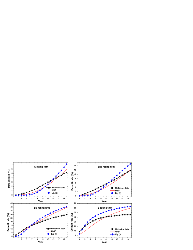
Figure 3: Historical (squares), theoretical (circles) and simulated (line) cumulative default rates for differently rated firms. All the simulations were performed with Monte Carlo runs $N=500,000$.

Table 2: The optimal bandwidth $h_{opt}$, parameters $\alpha$, $\beta$ for the true density estimate of differently rated firms. All the simulations were performed with Monte Carlo runs $N=500,000$.

	$\alpha$	$\beta$	Optimal bandwidth
A	0.206699	3	0.655522
Baa	0.219790	3	0.537277
Ba	0.252318	3	0.382729
B	0.327753	3	0.264402

Based on these results, we conclude that:

1. Simulations give similar or better results to the analytical results predicted by Eq. (3).

2. A- and Baa-rated firms have a smaller Brownian motion part. Their parameters $\sigma$ are much smaller than those of Ba- and B-rated firms.

3. The optimized parameters $\sigma$ of A- and Baa-rated firms are similar, but the jump parts $(\mu_{Z},\sigma_{Z})$ are different, which explains their different cumulative default rates and density functions. Indeed, Baa-rated firm may encounter more severe economic hazard (large jump-size) than A-rated firm.

4. As for Ba- and B-rated firms, except for the large $\sigma$, both of them have large $\mu_{Z}$ and especially large $\sigma_{Z}$, which indicate that the loss due to sudden economic hazard may fluctuate a lot for these firms. Hence, the large $\sigma$, $\mu_{Z}$ and $\sigma_{Z}$ account for their high default rates and low credit qualities.

5. From Fig. 2, we can conclude that the density functions of A- and Baa-rated firms still have the trend to increase, which means the default rates of A- and Baa-rated firms may increase little faster in future. As for Ba- and B-rated firms, their density functions have decreased, so their default rates may increase very slowly or be kept at a constant level. Mathematically speaking, the cumulative default rates of A- and Baa-rated firms are convex function, while the cumulative default rates of Ba- and B-rated firms are concave.

4.2 Correlated default

Our final example concerns with the default correlation of two firms. If we do not include jumps in the model, the default correlation can be calculated by using Eq. (3), (4) and (7). In Tables 3-6 we present comparisons of our results with those based on closed form solutions provided by Zhou (2001a) with $\rho=0.4$.

Table 3: One year default correlations (%). All the simulations are performed with the Monte Carlo runs $N=500,000$

	UNIF				Zhou (2001a)
	A	Baa	Ba	B	A	Baa	Ba	B
A	-0.01				0.00
Baa	-0.02	3.69			0.00	0.00
Ba	2.37	4.95	19.75		0.00	0.01	1.32
B	2.80	6.63	22.57	26.40	0.00	0.00	2.47	12.46

Table 4: Two year default correlations (%). All the simulations are performed with the Monte Carlo runs $N=500,000$

	UNIF				Zhou (2001a)
	A	Baa	Ba	B	A	Baa	Ba	B
A	2.35				0.02
Baa	2.32	4.25			0.05	0.25
Ba	4.17	7.17	20.28		0.05	0.63	6.96
B	4.73	8.23	23.99	29.00	0.02	0.41	9.24	19.61

Table 5: Five year default correlations (%). All the simulations are performed with the Monte Carlo runs $N=500,000$

	UNIF				Zhou (2001a)
	A	Baa	Ba	B	A	Baa	Ba	B
A	6.45				1.65
Baa	6.71	9.24			2.60	5.01
Ba	7.29	10.88	22.91		2.74	7.20	17.56
B	6.77	10.93	22.97	27.93	1.88	5.67	18.43	24.01

Table 6: Ten year default correlations (%). All the simulations are performed with the Monte Carlo runs $N=500,000$

	UNIF				Zhou (2001a)
	A	Baa	Ba	B	A	Baa	Ba	B
A	8.79				7.75
Baa	10.51	13.80			9.63	13.12
Ba	9.87	14.23	22.50		9.48	14.98	22.51
B	8.50	12.54	20.49	24.98	7.21	12.28	21.80	24.37

Next, let us consider the default correlations under the multivariate jump-diffusion processes. We use the following conditions in our multivariate UNIF method:

1. Setting $X(0)=2$ and $\ln(\kappa)=0$ for all firms.

2. Setting $\gamma=\mu$ and $\mu=-0.001$ for all firms.

3. Since we are considering two correlated firms, we choose $\sigma$ as,

   $$\sigma=\left[\begin{tabular}[]{cc}$\sigma_{11}$&$\sigma_{12}$\\ $\sigma_{21}$&$\sigma_{22}$\end{tabular}\right],$$ (30)

   where $\sigma\sigma^{\top}=H_{0}$ such that,

   $$\sigma\sigma^{\top}=H_{0}=\left[\begin{tabular}[]{cc}$\sigma_{1}^{2}$&$\rho_{12}\sigma_{1}\sigma_{2}$\\ $\rho_{12}\sigma_{1}\sigma_{2}$&$\sigma_{2}^{2}$\end{tabular}\right],$$

   and

   $$\left\{\begin{tabular}[]{l}$\sigma_{1}^{2}=\sigma_{11}^{2}+\sigma_{12}^{2}$,\\ $\sigma_{2}^{2}=\sigma_{21}^{2}+\sigma_{22}^{2}$,\\ $\rho_{12}=\displaystyle\frac{\sigma_{11}\sigma_{21}+\sigma_{12}\sigma_{22}}{\sigma_{1}\sigma_{2}}$.\end{tabular}\right.$$ (31)

   In Eq. (31), $\rho_{12}$ reflects the correlation of diffusion parts of the state vectors of the two firms. In order to compare with the standard Brownian motion and to evaluate the default correlations between different firms, we set all the $\rho_{12}=0.4$ as in Zhou (2001a). Furthermore, we use the optimized $\sigma_{1}$ and $\sigma_{2}$ in Table 1 for firm 1 and 2, respectively. Assuming $\sigma_{12}=0$, we get,

   $$\left\{\begin{tabular}[]{l}$\sigma_{11}=\sigma_{1}$,\\ $\sigma_{12}=0$,\\ $\sigma_{21}=\rho_{12}\sigma_{2}$,\\ $\sigma_{22}=\sqrt{1-\rho_{12}^{2}}\sigma_{2}$.\end{tabular}\right.$$

4. The arrival rate for jumps satisfies the Poisson distribution with intensity parameter $\lambda=0.1$ for all firms. The jump size is a normal distribution $Z_{t}\sim N(\mu_{Z_{i}},\sigma_{Z_{i}})$, where $\mu_{Z_{i}}$ and $\sigma_{Z_{i}}$ can be different for different firms to reflect specifics of the jump process for each firm. We adopt the optimized parameters given in Table 1.

5. As before, we generate the same interjump times $(T_{j}-T_{j-1})$ that satisfy an exponential distribution with mean value equals to 1 for each two firms.

We carry out the UNIF method to evaluate the default correlations via the following formula:

$$\rho_{12}(t)=\frac{1}{N}\sum_{n=1}^{N}\frac{P_{12,n}(t)-P_{1,n}(t)P_{2,n}(t)}{\sqrt{P_{1,n}(t)(1-P_{1,n}(t))P_{2,n}(t)(1-P_{2,n}(t))}},$$ (32)

where $P_{12,n}(t)$ is the probability of joint default for firms 1 and 2 in each Monte Carlo cycle, $P_{1,n}(t)$ and $P_{2,n}(t)$ are the cumulative default rates of firm 1 and 2, respectively, in each Monte Carlo cycle.

The simulated default correlations for one-, two-, five- and ten-years are given in Table 3-6. All the simulations were performed with the Monte Carlo runs $N=500,000$. Comparing those simulated default correlations with the theoretical data for standard Brownian motions, we can conclude that

1. Similarly to conclusions of Zhou (2001a), the default correlations of same rated firms are usually large compared to differently rated firms. Furthermore, the default correlations tend to increase over long horizons and may converge to a stable value.

2. In our simulations, the one year default correlations of (A,A) and (A,Baa) are negative. This is because they seldom default jointly during one year. Note, however, that the default correlations of other firms are positive and usually larger than the results in Zhou (2001a).

3. For two and five years, the default correlations of different firms increase. This can be explained by the fact that their individual first passage time density functions increase during these time horizon, hence the probability of joint default increases.

4. As for ten year default correlations, our simulated results are almost identical to the theoretical data for standard Brownian motions. The differences are that the default correlations of (Ba,Ba), (Ba,B) and (B,B) decrease from the fifth year to tenth year in our simulations. The reason is that the first passage time density function of Ba- and B-rated firms begin to decrease from the fifth year, hence the probability of joint default may increase slowly.

5 Conclusion

In this contribution, we have analyzed the credit risk problems of multiple correlated firms in the structural model framework, where we incorporated jumps to reflect the external shocks or other unpredicted events. By combining the fast Monte-Carlo method for one-dimensional jump-diffusion processes and the generation of correlated multidimensional variates, we have developed a fast Monte-Carlo type procedure for the analysis of multivariate and correlated jump-diffusion processes. The developed approach generalizes previously discussed non-correlated jump-diffusion cases for multivariate and correlated jump-diffusion processes. Finally, we have applied the developed technique to analyze the default events of multiple correlated firms via a set of historical default data. The developed methodology provides an efficient computational technique that is applicable in other areas of credit risk and pricing options.

References

- Ahangarani (2005) Ahangarani, P.M., Default Correlation with Considering Jumps. 2005. Available at Default Risk.com: http://www.defaultrisk.com/.
- Atiya et al (2005) Atiya, A.F. and Metwally, S.A.K., Efficient Estimation of First Passage Time Density Function for Jump-Diffusion Processes. SIAM Journal on Scientific Computing, 2005, 26, 1760–1775.
- Black et al (2005) Black, F. and M. Scholes, The Pricing of Options and Corporate Liabilities. Journal of Political Economy, 1973, 83, 637–659.
- Blake et al (1973) Blake, I. and Lindsey, W., Level-crossing problems for random processes. IEEE Trans. Inform. Theory, 1973, 19, 295–315.
- Chen (2005) Chen J.T., Using the sum-of-uniforms method to generate correlated random variates with certain marginal distribution. European Journal of Operational Research, 2005, 167, 226–242.
- Costa et al (1995) Costa, O. and Fragoso, M., Discrete time LQ-optimal control problems for infinite Markov jump parameter systems. IEEE Trans. Automat. Control, 1995, 40, 2076–2088.
- Devroye (1986) Devroye, L., Non-uniform Random Variate Generation, 1986 (Springer-Verlag: New York).
- Duffie et al (2000) Duffie, D., Pan, J. and Singleton, K., Transform Analysis and Option Pricing for Affine Jump-Diffusions. Econometrica, 2000, 68, 1343–1376.
- Hull et al (2001) Hull, J. and White, A., Valuing Credit Default Swaps II: Modeling Default Correlations. Journal of Derivatives, 2001, 8, 12–22.
- Jarrow et al (1997) Jarrow, R., Lando, D. and Turnbull, S., A Markov model for the term structure of credit spreads. Review of Financial Studies, 1997, 10, 481–523.
- Kloeden et al (2003) Kloeden, P.E., Platen, E. and Schurz, H., Numerical Solution of SDE Through Computer Experiments, Third Revised Edition, 2003 (Springer: Germany).
- Kou et al (2003) Kou, S.G. and Wang, H., First passage times of a jump diffusion process. Adv. Appl. Probab., 2003, 35, 504–531.
- Kuchler et al (2002) Kuchler, U. and Platen, E., Weak Discrete Time Approximation of Stochastic Differential Equations with Time Delay. Mathematics and Computing in Simulation, 2002, 59, 497–507.
- Liberati et al (2006) Liberati, N.B. and Platen, E., Strong Approximations of Stochastic Differential Equations with Jumps. Journal of Computational and Applied Mathematics, 2006, in press.
- Luciano et al (2005) Luciano, E. and Schoutens, W., A Multivariate Jump-Driven Financial Asset Model. ICER Applied Mathematics Working Paper No. 6-2005, 2005. Available at SSRN: http://ssrn.com/abstract=724709
- Metwally et al (2002) Metwally, S. and Atiya, A., Using brownian bridge for fast simulation of jump-diffusion processes and barrier options. The Journal of Derivatives, 2002, 10, 43–54.
- Merton (2005) Merton, R.C., Theory of rational option pricing. Bell Journal of Economics, 1973, 4, 141–183.
- Silverman (1986) Silverman, B.W., Density Estimation for Statistics and Data Analysis, 1986 (Chapman & Hall: London).
- Song et al (2006) Song J.H. and Kiureghian A.D., Joint First-Passage Probability and Reliability of Systems under Stochastic Excitation. Journal of Engineering Mechanics, 2006, 132(1), 65–77.
- Willemain et al (1993) Willemain, T.R. and Desautels, P.A., A method to generate autocorrelated uniform random numbers. Journal of Statistical Computation and Simulation, 1993, 45(1), 23–32.
- Wise et al (2004) Wise, M.B. and Bhansali, V., Correlated Random Walks and the Joint Survival Probability. 2004. Available at SSRN: http://ssrn.com/abstract=562207
- Zhang et al (2006) Zhang, D. and Melnik, R.V.N., First Passage Time for Multivariate Jump-diffusion Stochastic Models With Applications in Finance. Presented at the Sixth AIMS International Conference on Dynamical Systems and Differential Equations, University of Poitiers, Poitiers, France, 2006.
- Zhou (2001a) Zhou, C., An analysis of default correlation and multiple defaults. Review of Financial Studies, 2001, 14, 555–576.
- Zhou (2001b) Zhou, C., The Term Structure of Credit Spreads with Jump Risk. Journal of Banking and Finance, 2001, 25, 2015–2040.