First Passage Time for Multivariate Jump-diffusion Stochastic Models With Applications in Finance

Di Zhang and Roderick V.N. Melnik

Mathematical Modelling and Computational Sciences

Wilfrid Laurier University

Waterloo, ON, Canada N2L 3C5

Abstract. The “first passage-time” problem is an important problem with a wide range of applications in mathematics, physics, biology and finance. Mathematically, such a problem can be reduced to estimating the probability of a (stochastic) process first to reach a critical level or threshold. While in other areas of applications the FPT problem can often be solved analytically, in finance we usually have to resort to the application of numerical procedures, in particular when we deal with jump-diffusion stochastic processes (JDP). In this paper, we develop a Monte-Carlo-based methodology for the solution of the FPT problem in the context of a multivariate jump-diffusion stochastic process. The developed methodology is tested by using different parameters, the simulation results indicate that the developed methodology is much more efficient than the conventional Monte Carlo method, which establishes itself as an efficient tool for further practical applications, such as the analysis of default correlation and predicting barrier options in finance.

1. Introduction

In a jump-diffusion process (JDP), the dynamics of underlying process have two random components: a continuous diffusion component and a discontinuous jump component [1], in which the jump component can be explained as a sudden drop of process’s value. The first passage time (FPT) problem for jump-diffusion processes has Attracted attention of researchers in such diverse fields as queuing networks [2], computer vision [3], target recognition [4]. In the financial world, many problems also require the information on the first passage time of a stochastic process, for example, in modeling credit risk and valuing defaultable securities [1], or in predicting barrier options [8]. Furthermore, it is now generally accepted that the geometric Brownian motion model for market behavior may produce misleading results in [1, 9], such as mismatching credit spreads on corporate bonds, underlying derivative prices. Jump-diffusion processes have established themselves as a sound alternative to the geometric Brownian motion model.

However, if we consider jumps in the process, except for very basic process types where closed form solutions are available, when the jump sizes are doubly exponential or exponentially distributed [5], or when the jumps can have only nonnegative values (assuming that the crossing boundary is below the process starting value) [6], where closed form solutions are available, for most problems we can only resort to the numerical procedures.

Monte Carlo simulation is a very promising candidate in dealing with FPT problems. However, in conventional Monte Carlo method, in order to avoid discretization bias [7], we need to discretize the time horizon into small enough intervals, and to evaluate the process at each discretized time that is very time-consuming. Recently, Atiya and Metwally [8, 9] have developed a fast Monte Carlo-type numerical method to solve the FPT problem for jump-diffusion process.

In many financial problems we have to deal with multiple processes in practice and consider their jointly crossing the critical level, so it is very useful to develop fast numerical procedure for multivariate jump-diffusion process. In this contribution, we extend the fast Monte Carlo-type numerical methodology to the more general case that covers affine multivariate processes jump-diffusion. The developed methodology can be easily extended to other financial applications and areas where FPT problem arises.

The article is organized as follows: section 2 describes our mathematical model. The algorithms are presented in section 3 and simulation results are given in section 4. Concluding remarks are given section 5.

2. Mathematical Model

In this section, first, we give brief discussion on the affine jump-diffusion model, then we deduce the first passage time distribution under multivariate jump-diffusion process. At last, we consider the issue of kernel estimator.

2.1. Affine jump-diffusion

Affine jump-diffusion is a jump-diffusion process for which the drift vector, “instantaneous” covariance matrix and jump intensities all have affine dependence on the state vector.

Let us consider a complete probability space $(\Omega,F,P)$ and an information filtration $(F_{t})$, and suppose that $X$ is a Markov process in some state space $D\subset\mathbb{R}^{n}$, solving the stochastic differential equation [10]

$$dX_{t}=\mu(X_{t})dt+\sigma(X_{t})dW_{t}+dZ_{t},$$ (1)

where $W$ is an $(F_{t})$-standard Brownian motion in $\mathbb{R}^{n}$; $\mu:D\rightarrow\mathbb{R}^{n}$, $\sigma:D\rightarrow\mathbb{R}^{n\times n}$, and $Z$ is a pure jump process whose jumps have a fixed probability distribution $\nu$ on $\mathbb{R}^{n}$ and arrive with intensity $\{\lambda(X_{t}):t\geq 0\}$, for some $\lambda:D\rightarrow[0,\infty)$.

Definition 1.

The above model is an affine model if [10]:

$$\mu(X_{t},t)=K_{0}+K_{1}X_{t}$$

$$(\sigma(X_{t},t)\sigma(X_{t},t)^{\top})_{ij}=(H_{0})_{ij}+(H_{1})_{ij}X_{j}$$

$$\lambda(X_{t})=l_{0}+l_{1}\cdot X_{t},$$ (2)

where $K=(K_{0},K_{1})\in\mathbb{R}^{n}\times\mathbb{R}^{n\times n}$, $H=(H_{0},H_{1})\in\mathbb{R}^{n\times n}\times\mathbb{R}^{n\times n\times n}$, $l=(l_{0},l_{1})\in\mathbb{R}^{n}\times\mathbb{R}^{n\times n}$ and the “jump transform” (determines the jump-size distribution) $\psi(c)=\int_{\mathbb{R}^{n}}\exp(c,z)d\nu(z)$, for $c\in\mathbb{C}^{n}$, is known whenever the integral is well defined. The “coefficients” $(K,H,l,\psi)$ of $X$ completely determine its distribution.

2.2. First passage time distribution

Now, we will consider the first passage time distribution in the context of multiple processes. In order to obtain a computable multi-dimensional solutions of FPT distribution, we need to simplify Eq. (1) and (2)based on the following assumptions:

1. Each $W_{t}$ in Eq. (1) is independent;

2. $K_{1}=0$, $H_{1}=0$ and $l_{1}=0$ that means the drift term, the diffusion process (Brownian motion) and the arrival intensity are independent with state vector $X$;

3. The distribution of jump-size $Z_{t}$ is also independent with $X$.

In this scenario, we can rewrite Eq. (1) as

$$dX_{t}=\mu dt+\sigma dW_{t}+dZ_{t},$$ (3)

where

$$\mu=K_{0},\;\sigma\sigma^{\top}=H_{0},\;\lambda=l_{0}.$$

Atiya et al. [9] have deduced one-dimensional first passage time distribution in time horizon $[0,T]$. In order to judge multiple processes, from Eq. (3), we obtain multi-dimensional formulas and simplify them into computable formulas. We will highlight the main steps of our procedure below.

As defined, the multiple processes $X$ can be written as $X=[X_{1},X_{2},\dots]^{\top}$. Let us consider one of its components, a sub-process $X_{i}$ that satisfies the following stochastic differential equation:

$$dX_{i} = \mu_{i}dt+\sum_{j}\sigma_{ij}dW_{j}+dZ_{i}$$ (4)

$$= \mu_{i}dt+\sigma_{i}dW_{i}+dZ_{i},$$

where $W_{i}$ is also a standard Brownian motion and $\sigma_{i}$ is:

$$\sigma_{i}=\sqrt{\sum_{j}\sigma_{ij}^{2}}.$$

We assume that in the interval $[0,T]$, $M_{i}$ times of jumps happen for $X_{i}$. Let the jump instants be $T_{1},T_{2},\cdots,T_{M_{i}}$. Let $T_{0}=0$ and $T_{M_{i}+1}=T$. $\tau_{j}$ equals interjump times, which is $T_{j}-T_{j-1}$. Following the notation of [9], let $X_{i}(T_{j}^{-})$ be the process value immediately before the $j$th jump, and $X_{i}(T_{j}^{+})$ be the process value immediately after the $j$th jump. The jump-size is then $X_{i}(T_{j}^{+})-X_{i}(T_{j}^{-})$, and we can use this jump-size to generate $X_{i}(T_{j}^{+})$ sequentially.

If we define $A_{i}(t)$ as the event that process crossed the threshold $D_{i}(t)$ for the first time in the interval $[t,t+dt]$, we have

$$g_{ij}(t)=p(A_{i}(t)\in dt|X_{i}(T_{j-1}^{+}),X_{i}(T_{j}^{-})).$$ (5)

If we only consider one interval $[T_{j-1},T_{j}]$, we can obtain [11, 12]

$$g_{ij}(t) = \frac{X_{i}(T_{j-1}^{+})-D_{i}(t)}{2y_{i}\pi\sigma_{i}^{2}}(t-T_{j-1})^{-\frac{3}{2}}(T_{j}-t)^{-\frac{1}{2}}$$ (6)

$$*\exp\left(-\frac{[X_{i}(T_{j}^{-})-D_{i}(t)-\mu_{i}(T_{j}-t)]^{2}}{2(T_{j}-t)\sigma_{i}^{2}}\right)$$

$$*\exp\left(-\frac{[X_{i}(T_{j-1}^{+})-D_{i}(t)+\mu_{i}(t-T_{j-1})]^{2}}{2(t-T_{j-1})\sigma_{i}^{2}}\right),$$

where

$$y_{i}=\frac{1}{\sigma_{i}\sqrt{2\pi\tau_{j}}}\exp\left(-\frac{[X_{i}(T_{j-1}^{+})-X_{i}(T_{j}^{-})+\mu_{i}\tau_{j}]^{2}}{2\tau_{j}\sigma_{i}^{2}}\right).$$

After getting result in one interval, we combine the results to obtain the density for the whole interval $[0,T]$. Let $B(s)$ be a Brownian bridge in the interval $[T_{j-1},T_{j}]$, with $B(T_{j-1}^{+})=X_{i}(T_{j-1}^{+})$, $B(T_{j}^{-})=X_{i}(T_{j}^{-})$, the probability that the minimum of $B(s_{i})$ is always above the boundary level is [13]

$$P_{ij} = P\left(\inf_{T_{j-1}\leq s_{i}\leq T_{j}}B(s_{i})>D_{i}(t)|B(T_{j-1}^{+})=X_{i}(T_{j-1}^{+}),B(T_{j}^{-})=X_{i}(T_{j}^{-})\right)$$ (9)

$$= \left\{\begin{array}[]{ll}1-\exp\left(-\frac{2[X_{i}(T_{j-1}^{+})-D_{i}(t)][X_{i}(T_{j}^{-})-D_{i}(t)]}{\tau_{j}\sigma_{i}^{2}}\right),&\mathrm{if}\;X_{i}(T_{j}^{-})>D_{i}(t),\\ 0,&\mathrm{otherwise}.\end{array}\right.$$

Then $B(s_{i})$ is below the threshold level, which means the default happens or already happened, and its probability is $1-P_{ij}$. Then let $L(s_{i})\equiv L_{i}$ denote the index of the interjump period in which the time $s_{i}$ falls in $[T_{L_{i}-1},T_{L_{i}}]$. Also let $I_{i}$ represent the index of the first jump, which happened in simulated jump instant.

$$I_{i} = \min(j:X_{i}(T_{k}^{-})>D_{i}(t);k=1,\ldots,j,\;\mathrm{and}$$ (10)

$$\;\;\;\;\;\;\;\;\;\;\;\>X_{i}(T_{k}^{+})>D_{i}(t);k=1,\ldots,j-1,\;\mathrm{and}\;X_{i}(T_{j}^{+})\leq D_{i}(t)).$$

If no such $I_{i}$ exists, we set $I_{i}=0$.

Then we get the probability of the interval $[0,T]$

$$P(A_{i}(s_{i})\in ds|X_{i}(T_{j-1}^{+}),X_{i}(T_{j}^{-}),j=1,\ldots,M_{i}+1)$$ (14)

$$= \left\{\begin{array}[]{ll}g_{iL_{i}}(s_{i})\prod_{k=1}^{L_{i}-1}P_{ik}&\mathrm{if}\;L_{i}<I_{i}\;\mathrm{or}\;I_{i}=0,\\ g_{iL_{i}}(s_{i})\prod_{k=1}^{L_{i}-1}P_{ik}+\prod_{k=1}^{L_{i}}P_{ik}\delta(s_{i}-T_{I_{i}})&\mathrm{if}\;L_{i}=I_{i},\\ 0&\mathrm{if}\;L_{i}>I_{i},\end{array}\right.$$

where $\delta$ is the Dirac’s delta function.

2.3. The kernel estimator

For each $X_{i}$, after generating series of first passage times $s_{i}$, we use a kernel density estimator with a Gaussian kernel to estimate the first passage time density (FPTD) $f$. As described in [9], the kernel density estimator is based on centering a kernel function of a bandwidth as follows:

$$\widehat{f}=\frac{1}{N}\sum_{i=1}^{N}K(h,t-s_{i}),$$ (15)

where

$$K(h,t-s_{i})=\frac{1}{\sqrt{\pi/2}h}\exp\left(-\frac{(t-s_{i})^{2}}{h^{2}/2}\right).$$ (16)

The optimal bandwidth in the kernel function $K$ can be calculated as [15]:

$$h_{opt}=\left(2N\sqrt{\pi}\int_{-\infty}^{\infty}(f_{t}^{\prime\prime})^{2}dt\right)^{-0.2},$$ (17)

where $N$ is the number of generated points and $f_{t}$ is true density. Here we use the approximation for the distribution as a gamma distribution as proposed in [9]:

$$f_{t}=\frac{\alpha^{\beta}}{\Gamma(\beta)}t^{\beta-1}\exp(-\alpha t).$$ (18)

In this case the functional becomes

$$\int_{0}^{\infty}(f_{t}^{\prime\prime})^{2}dt=\sum_{i=1}^{5}\frac{W_{i}\alpha_{i}\Gamma(2\beta-i)}{2^{(2\beta-i)}(\Gamma(\beta))^{2}},$$ (19)

where

$$W_{1}=A^{2},\;\;W_{2}=2AB,\;\;W_{3}=B^{2}+2AC,\;\;W_{4}=2BC,\;\;W_{5}=C^{2},$$

and

$$A=\alpha^{2},\;\;B=-2\alpha(\beta-1),\;\;C=(\beta-1)(\beta-2).$$

From Eq. (19), apparently, in order to get a nonzero bandwidth, we has constrained $\beta$ to be at least equal to 3. Using this constraint, we can obtain the estimates of the parameters $\alpha$ and $\beta$ via the method of moments: $\overline{t}=\widehat{E}(t)=\frac{1}{N}\sum_{i=1}^{N}t_{i}$ and $\widehat{E}(t^{2})=\frac{1}{N}\sum_{i=1}^{N}t_{i}^{2}$ and the sample standard deviation is $\zeta=\sqrt{\widehat{E}(t^{2})-\overline{t}^{2}}$. The estimates are $\widehat{\alpha}=\frac{\overline{t}}{\zeta^{2}}$ and $\widehat{\beta}=\frac{\overline{t}^{2}}{\zeta^{2}}\geq 3$.

The kernel estimator can be easily generalized to the multivariate case. Suppose we consider $X=[X_{1},X_{2},\dots,X_{m}]^{\top}$, let $\overrightarrow{t}=[t_{1},t_{2},\dots,t_{m}]$, and $\overrightarrow{s_{i}}=[s_{1i},s_{2i},\dots,s_{mi}]$, $s_{ji}(j=1,2,\dots,m)$ is the first passage time for $X_{j}$. Then, the multivariate kernel density estimator with kernel $K$ and window width $h$ is defined by [15]

$$\widehat{f}(\overrightarrow{t})=\frac{1}{N}\sum_{i=1}^{N}K\left[h,(\overrightarrow{t}-\overrightarrow{s_{i}})\right],$$ (20)

where

$$K(\overrightarrow{t})=(2\pi h^{2})^{-m/2}\exp\left(-\frac{1}{2h^{2}}\overrightarrow{t}^{\top}\overrightarrow{t}\right).$$ (21)

And if we approximate the true density $f$ as a unit $m$-variate normal density, then the optimal bandwidth $h_{opt}$ is [15]

$$h_{opt}=\frac{1}{N^{1/(m+4)}}\left[\frac{4}{2m+1}\right]^{1/(m+4)}.$$ (22)

3. Algorithms

In section 2, we have built up a multivariate jump-diffusion model as describe in Eq. (3), and its first passage time distribution was also obtained in section 2.2. In this section, we will discuss how to simulate the multivariate jump-diffusion process efficiently via Monte Carlo method. In conventional Monte Carlo method, the simulation is very straightforward, we divide the time horizon $[0,T]$ into $n$ small intervals $[0,t_{1}]$, $[t_{1},t_{2}]$, $\cdots$, $[t_{n-1},T]$ and in each Monte Carlo run, we need to calculate the value of $X_{i}$ at each discretized time $t$. We should mention that in order to exclude discretization bias, the number $n$ must be large enough. It is obvious that this conventional method is very time-consuming.

Recently, Atiya and Metwally [8, 9] have proposed two fast Monte Carlo type methods, which are about 10-30 times faster than the conventional Monte Carlo approach. We called them uniform sampling (UNIF) method, which involves sampling using uniform distribution, and inverse Gaussian density sampling (IG) method, which uses inverse Gaussian density method for sampling.

In this article, we mainly focus on the uniform sampling (UNIF) method and extend it to the multivariate jump-diffusion process. The major improvement of UNIF method is that it only evaluate $X_{i}$ at generated jump instants and between each two jumps the process is a Brownian bridge, so we just consider the probability of $X_{i}$ crossing the boundary level in $(T_{j-1},T_{j})$ instead of evaluating $X_{i}$ at each discretized time $t$. More exactly, we assume that the values of $X_{i}(T_{j-1}^{+})$ and $X_{i}(T_{j}^{-})$ are known as two end points of Brownian bridge, we generate a variable $s_{i}$ with uniform distribution and by using Eq. (9) to see whether $X_{i}(s_{i})$ is smaller than the threshold level, if it defaults, then we have successfully generated a first passage time $s_{i}$ and can neglect the other intervals and perform another Monte Carlo run.

In [8, 9], the jump-diffusion process is involved in a univariate model. However, our model is based on multivariate process in which $X_{i}$ are correlated as described in Eq. (3), so we need to consider several points as follows:

1. In this article, as a first step, we assume that the arrival rate $\lambda$ for the Poisson jump process and the distribution of $(T_{j}-T_{j-1})$ are the same for each $X_{i}$. As for jump-size, we should generate them as given distribution, and it can be different to reflect the different jump process for each $X_{i}$.

2. At present, we use exponential distribution (mean value $\mu_{T}$) for $(T_{j}-T_{j-1})$ and normal distribution (mean value $\mu_{J}$ and standard deviation $\sigma_{J}$) for the jump-size. Of course, we can use any distribution as desired.

3. If we consider $m$ processes, i.e., $X=[X_{1},X_{2},\dots,X_{m}]^{\top}$, then we need an array IsDefault (whose size is $m$) to indicate whether process $X_{i}$ has crossed the threshold in this Monte Carlo run. If $X_{i}$ has crossed, then we set IsDefault$(i)=1$, and will not evaluate it during this Monte Carlo run.

Next, we will give a description of our algorithm, based on a multivariate extension of the algorithms proposed in [8, 9].

3.1. Uniform sampling method

Let us consider $m$ processes in the given time horizon $[0,T]$, as described above, we have generated the jump instant $T_{j}$ by generating interjump times $(T_{j}-T_{j-1})$, besides we set IsDefault$(i)=0(i=1,2,\cdots,m)$ at first.

From Eq. (4), we can see that,

1. If jump doesn’t occur, the diffusion follows a standard Brownian motion, $W_{i}(T)\sim N(0,T)$, so interjump size $(X_{i}(T_{j}^{-})-X_{i}(T_{j-1}^{+}))$ follows a normal distribution of mean $\mu_{i}(T_{j}-T_{j-1})$ and standard deviation $\sigma_{i}\sqrt{T_{j}-T_{j-1}}$. After extend if necessary, we get

   $$X_{i}(T_{j}^{-})\sim X_{i}(T_{j-1}^{+})+\mu_{i}(T_{j}-T_{j-1})+\sum_{k=1}^{m}\sigma_{ik}N(0,T_{j}-T_{j-1}),$$

   and the initial state is $X_{i}(0)=X_{i}(T_{0}^{+})$.

2. If jump occurs, the jump-size and direction of $Z_{i}(T_{j})$ are not fixed either. We simulate the jump-size by a normal distribution, and of course we may generate it according to other distribution. Then we can compute the postjump value:

   $$X_{i}(T_{j}^{+})=X_{i}(T_{j}^{-})+Z_{i}(T_{j}).$$

After generating beforejump and postjump value $X_{i}(T_{j}^{-})$ and $X_{i}(T_{j}^{+})$ ($j=1,\cdots,M$, $M$ is the total number of jumps for all the processes $X_{i}$), we can compute $P_{ij}$ according to Eq. (9). To recur the first passage time density (FPTD) $f_{i}(t)$, we need to consider three conditions for each $X_{i}$ that is still above the threshold:

1. First passage happens inside the interval. We know if $X_{i}(T_{j-1}^{+})>D_{i}(t)$, $X_{i}(T_{j}^{-})<D_{i}(t)$, then the first passage happened in the time interval $[T_{j-1},T_{j}]$. To judge when the first passage happen, first we compute the probability $P_{ij}$ of $X_{i}$ always above the threshold according to Eq. (9), then we generate $s_{i}$ as $s_{i}=b_{ij}u_{i}+T_{j-1}$, where $b_{ij}=\frac{T_{j}-T_{j-1}}{1-P_{ij}}$, and $u_{i}$ is a uniform random number in $[0,1]$. If $s_{i}$ also belongs to interval $[T_{j-1},T_{j}]$, then the first passage time occurred in this interval, where $s_{i}$ is the first passage time and now we set IsDefault$(i)=1$ to indicate process $X_{i}$ has crossed the critical level. In this condition, we can get conditional interjump first passage time density of that specific interval by Eq.(6). To get the density of whole interval $[0,T]$, we have $\widehat{f}_{i,n}(t)=\left(\frac{T_{j}-T_{j-1}}{1-P_{ij}}\right)g_{ij}(s_{i})*K(h_{opt},t-s_{i})$, where $n$ is the iteration number of Monte Carlo cycle.

2. First passage doesn’t happen in this interval. If $s_{i}$ doesn’t belong to interval $[T_{j-1},T_{j}]$, then the first passage time has not yet occur in this interval.

3. First passage happens in the right boundary of interval. If $X_{i}(T_{j}^{+})<D_{i}(t)$, $X_{i}(T_{j}^{-})>D_{i}(t)$, which follow the definition in Eq. (10), then obviously $T_{I_{i}}$ (set $I_{i}=j$) is the first passage time. Evaluate the density function using kernel function $\widehat{f}_{i,n}(t)=K(h_{opt},t-T_{I_{i}})$, and set IsDefault$(i)=1$.

Then we increase $j$ and examine the next interval and judge these three conditions for each non-crossing process $X_{i}$ again. For each Monte Carlo run, if we make a rough assumption that the probability of $X_{i}$ crossing the threshold is not correlated, then we can obtain the multivariate FPTD as $\widehat{f}_{n}(\overrightarrow{t})=\Pi_{i=1}^{m}\left(\frac{T_{j}-T_{j-1}}{1-P_{ij}}\right)g_{ij}(s_{i})*K(h_{opt},\overrightarrow{t}-\overrightarrow{s})$.

After running $N$ times of Monte Carlo cycle, we get the one-dimensional FPTD of $X_{i}$ as $\widehat{f}_{i}(t)=\frac{1}{N}\sum_{n=1}^{N}\widehat{f}_{i,n}(t)$, and multivariate FPTD as $\widehat{f}(\overrightarrow{t})=\frac{1}{N}\sum_{n=1}^{N}\widehat{f}_{n}(\overrightarrow{t})$

4. Simulation results

In this section, as a demonstration, we will test the multivariate UNIF method on two-dimensional case. In order to check the efficient and validity of the UNIF method, we use three examples with different arrival rate $\lambda=1,3,8$ for the Poisson jump process to judge the efficiency of our algorithms. The parameters are as follows

$$X_{0}=[0,0]^{\top},\;D(t)=[\ln(0.9)-0.002t,\ln(0.95)-0.012t]^{\top}$$

$$\mu=[-0.002,-0.012]^{\top},\;\sigma=\left[\begin{tabular}[]{cc}$0.2$&$0.0$\\ $0.0$&$0.2$\end{tabular}\right],$$

$$\mu_{Z}=[0,0]^{\top},\;\sigma_{Z}=[0.2,0.12]^{\top}.$$

where $X_{0}$ is the starting value for the process, $D_{(}t)$ is the threshold, $\mu$ is the constant instantaneous drift, $\sigma$ represents the Brownian motion, and $\mu_{Z}$ and $\sigma_{Z}$ are the mean and standard deviations, respectively, of the jump sizes.

The simulation was carried out with total Monte Carlo runs $N=500,000$ in horizon $[0,1]$. Moreover, we have also carried out conventional Monte Carlo simulation with the same parameters, the estimated density functions are displayed in Fig. 1-3. All the simulations were carried out on a 2.4 GHz AMD Opteron(tm) Processor. The optimal bandwidth and CPU time are described in Table 1.

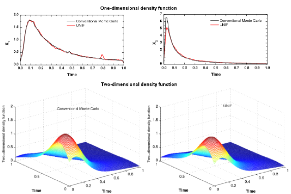
Figure 1. Example 1 ($\lambda=1$): One-dimensional (top) and two-dimensional density function (bottom) estimate using $100,000$ iterations for UNIF and conventional Monte Carlo approaches. The discretization size of time horizon is $\Delta=0.0002$ for conventional Monte Carlo method.

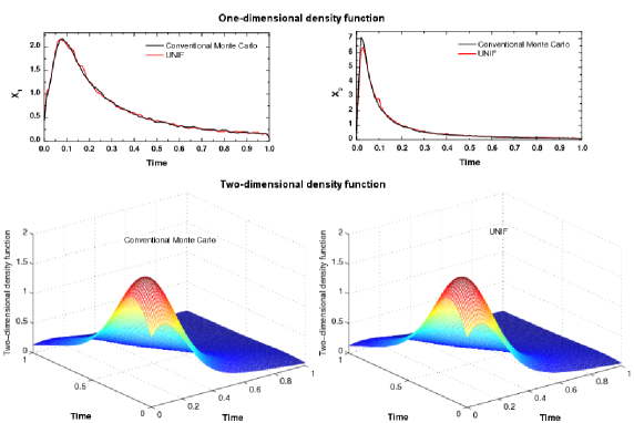
Figure 2. Example 2 ($\lambda=3$): One-dimensional (top) and two-dimensional density function (bottom) estimate using $100,000$ iterations for UNIF and conventional Monte Carlo approaches. The discretization size of time horizon is $\Delta=0.0002$ for conventional Monte Carlo method.

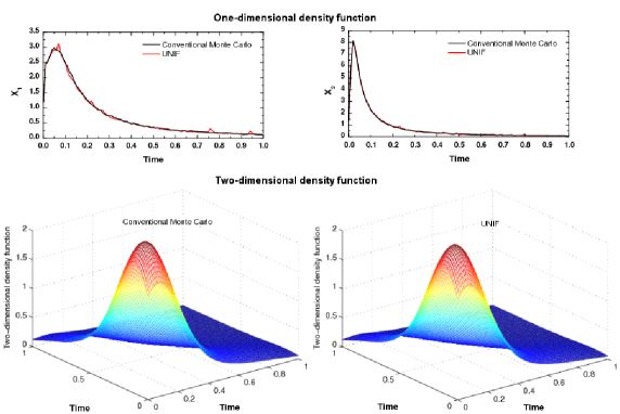
Figure 3. Example 3 ($\lambda=8$): One-dimensional (top) and two-dimensional density function (bottom) estimate using $100,000$ iterations for UNIF and conventional Monte Carlo approaches. The discretization size of time horizon is $\Delta=0.0002$ for conventional Monte Carlo method.

From Fig. 1-3, we can see that the multivariate UNIF method gives similar density function as the conventional one, that check the validity of our algorithms. An interesting phenomenon is that increasing $\lambda$ will affect FPTD of $X_{1}$ a lot whose probability of crossing the threshold is low in the interval $[0,T]$.

Table 1. The optimal bandwidth $h_{opt}$, and CPU time per Monte Carlo run of the simulations. The first $h_{opt}$ is for $X_{1}$ and the second for $X_{2}$. All the simulations were performed with Monte Carlo runs $N=100,000$, besides, for conventional Monte Carlo (CMC) method, the discretization size of time horizon is $\Delta=0.0002$.

		Optimal bandwidth		CPU time
		$X_{1}$	$X_{2}$
Example 1	CMC	0.012664	0.006943	0.286642
	UNIF	0.016030	0.013880	0.000527
Example 2	CMC	0.011157	0.006582	0.284554
	UNIF	0.012249	0.009443	0.000731
Example 3	CMC	0.008894	0.005921	0.299156
	UNIF	0.009117	0.006542	0.001222

Undoubtedly, from Table 1, one can easily realizes that the multivariate UNIF approach is much more efficient than the conventional one, which establish it as a fast methodology for practical applications.

5. Conclusion

In summary, we have studied the first passage time problem in the context of multivariate jump-diffusion processes. We have extended the fast Monte Carlo-type numerical method - the UNIF method – to multiple processes. From our simulation results, we can see that the multivariate UNIF approach is much more efficient than the conventional Monte Carlo method, which illustrates that the developed methodology can provide an efficient tool for further practical applications, such as the analysis of default correlation and predicting barrier options in finance.

Acknowledgements. We would like to thank NSERC for its support.

Received Month Year; Sep.29, 2006.

References

- [1] C. Zhou, The Term Structure of Credit Spreads with Jump Risk, Journal of Banking and Finance 25 (2001), 2015–2040.
- [2] G. Gorov, Ya. Kogan and N. Paradizov, Jump diffusion approximation in single-server systems with interruption of service and variable rate of arrival of calls, Avtomatika i Telemekhanika, 6 (1985), 44–51.
- [3] S. C. Zhu, Stochastic jump-diffusion process for computing medial axes in Markov random fields, IEEE Trans. Pattern Analysis and Machine Intelligence, 21 (1999), 1158–1169.
- [4] M. Miller, U. Grenander, J. O’Sullivan and D. Snyder, Automatic target recognition organized via jump-diffusion algorithm, IEEE Trans. Image Processing, 6 (1997), 157–174.
- [5] S.G. Kou, H. Wang, First passage times of a jump diffusion process, Adv. Appl. Probab. 35 (2003), 504–531.
- [6] I. Blake, W. Lindsey, Level-crossing problems for random processes, IEEE Trans. Inform. Theory IT-19 (1973), 295–315.
- [7] P.E. Kloeden, E. Platen, H. Schurz, “Numerical Solution of SDE Through Computer Experiments”, Third Revised Edition, Springer, Germany, 2003.
- [8] S. Metwally, A. Atiya, Using brownian bridge for fast simulation of jump-diffusion processes and barrier options, The Journal of Derivatives 10 (2002), 43–54.
- [9] A.F. Atiya, S.A.K. Metwally, Efficient Estimation of First Passage Time Density Function for Jump-Diffusion Processes, SIAM Journal on Scientific Computing 26 (2005), 1760–1775.
- [10] D. Duffie, J. Pan, K. Singleton, Transform Analysis and Option Pricing for Affine Jump-Diffusions, Econometrica 68 (2000), 1343–1376.
- [11] W. Feller, “An Introduction to Probability Theory and Its Applications”, Vol. 1, Wiley, New York, 1968.
- [12] L.C.G. Rogers and D. Williams, “Diffusions, Markov Processes and Martingales”, Vol. 1, Wiley, New York, 1994.
- [13] I. Karatzas and S. Shreve, “Brownian Motion and Stochastic Calculus”, Springer-Verlag, New York, 1991.
- [14] O. Costa, M. Fragoso, Discrete time LQ-optimal control problems for infinite Markov jump parameter systems, IEEE Trans. Automat. Control 40 (1995), 2076–2088.
- [15] B.W. Silverman, “Density Estimation for Statistics and Data Analysis”, Chapman & Hall, London, 1986.
- [16] L. Devroye, “Non-uniform Random Variate Generation”, Springer-Verlag, New York, 1986.