Simulation of Phase Combinations in Shape Memory
Alloys Patches by Hybrid Optimization Methods

Abstract

In this paper, phase combinations among martensitic variants in shape memory alloys patches and bars are simulated by a hybrid optimization methodology. The mathematical model is based on the Landau theory of phase transformations. Each stable phase is associated with a local minimum of the free energy function, and the phase combinations are simulated by minimizing the bulk energy. At low temperature, the free energy function has double potential wells leading to non-convexity of the optimization problem. The methodology proposed in the present paper is based on an initial estimate of the global solution by a genetic algorithm, followed by a refined quasi-Newton procedure to locally refine the optimum. By combining the local and global search algorithms, the phase combinations are successfully simulated. Numerical experiments are presented for the phase combinations in a SMA patch under several typical mechanical loadings.

and

1 Introduction

Shape Memory Alloys (SMA) are materials with increasing range of applications in engineering, aerosapce, and biomedical industries. They possess unique properties of being able to recover their original shape after permanent deformations. These materials can directly transduce thermal energy into mechanical and vice versa. The key to “pseudo-elastic” behaviour of these materials and the “shape memory effect” [8, 26] is held by the first-order martensitic phase transformations in these materials. Indeed, drastic changes in their properties are originated from their microstructure or phase combinations. Via the phase transformation, the microstructure of the material can be switched among various combinations between austenite, martensite variants, or their mixtures. Austenitic phase is a more symmetric phase of the crystallic lattice, prevailing at high temperature, while martensite is a less symmetric, low-temperature phase [1, 8, 26]. Between these two critical situations, austenite and martensite might co-exist providing a typical example of phase combinations. Upon external loading, one phase combination can be switched to another. If the material is constrained at the boundary, a specific (“self-accommodating”) combination of different phases will be established such that the bulk energy in the constrained domain will be minimized [1, 18, 19].

The mathematical framework for modeling phase combinations in shape memory materials is based on the solution of the variational problem with respect to a frame-indifferent non-convex free energy function $\phi(Y,\theta)$ ([5, 6, 11, 19, 18] and references therein) :

$$W(Y)=\int_{\Omega}\phi(Y,\theta)dV,$$ (1)

where $\Omega$ is the reference configuration associated with the considered material, $Y$ is the deformation tensor, and $\theta$ is the temperature of the material. Hence, by minimizing $W(Y)$ from (1), we minimize the bulk energy of the considered structure, as a functional of the deformation tensor, at temperature $\theta$. This procedure, performed particularly often at the mesoscale [7, 10, 11, 19, 18], has several known difficulties. It is known that in the general case the variational problem given by Eq.(1) may have infinitely many minimizers ([7, 19, 10] and references therein). On the other hand, a more precise definition of the free energy that allow us to account for interfacial energy effects by introducing gradients of the order parameters is a highly non-trivial task ([1, 18] and references therein) connected with additional difficulties. The problem can also be regularized by assigning simplified, e.g. affine, boundary conditions. For example, for the simulation of simple laminated microstructure, the affine boundary conditions are constructed by assuming that the deformation gradient of the material on the domain boundary is a linear combination of its equilibrium deformation gradients:

$$Y(x)=(\lambda F_{0}+(1-\lambda)RF_{1})x,\,x\in\partial\Omega,$$ (2)

where $R$ is a rotation matrix satisfying a twinning equation (see [7, 10, 11, 19]) and $\lambda$ is the thickness of layers in the laminated microstructure. $F_{0}$ and $F_{1}$ are the deformation gradients that minimize the local energy function (for square to rectangular transformation) when the deformation gradient $\nabla Y$ takes any of the following following values:

$$F_{0}=\left(\begin{array}[]{cc}1+e_{m}/\sqrt{2}&0\\ 0&1-e_{m}/\sqrt{2}\end{array}\right), F_{1}=\left(\begin{array}[]{cc}1-e_{m}/\sqrt{2}&0\\ 0&1+e_{m}/\sqrt{2}\end{array}\right),$$ (7)

where $e_{m}$ is a local minimum of the free energy function $\phi(Y,\theta)$. In the general case, however, the above affine boundary conditions may not be appropriate.

In solving problem (1), we have to face also numerical challenges connected with several local minima, resulted from phase mixtures under low and moderate temperature regimes, and non-convexity of the problem ([4, 10, 19, 30] and references therein). Minimization procedures based on conventional local search methods with randomly chosen initial guesses [9] may not lead to a satisfactory result in those cases where the solution space is discretized with a large number of node points.

In the present paper, we construct a mathematical model for the simulation of phase combinations in SMA materials on the basis of the Landau theory. We associate the phase combination with the global minimizer of the bulk energy of the SMA structure with the prescribed mechanical boundary conditions. We develop a hybrid optimization strategy consisting of two main steps. Firstly, we apply the Genetic Algorithm (GA) and its global exploration capacity to obtain an initial estimation of the global minimizer. Then, we apply the quasi-Newton method to refine such an estimation locally. Finally, the developed procedure is demonstrated by several numerical examples simulating phase combinations in SMA materials.

2 Landau Free Energy Function and Variational Formulation

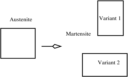
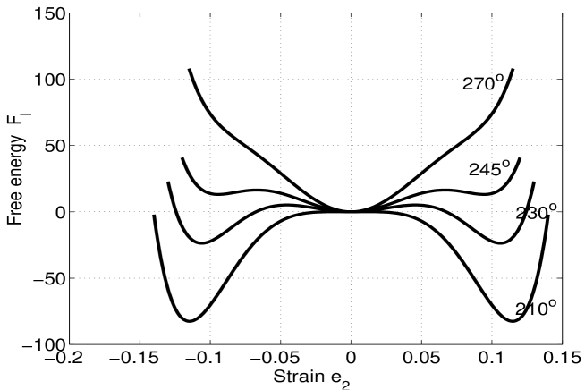
Figure 1: (a) Sketch of the square to rectangular transformation, (b) The temperature dependency of the free energy function for the transformation.

For the modeling of phase combinations in SMAs structures, the first task is to characterize different phases, which is different from one material to another. Here our mathematical model will be based on the square to rectangular transformations. In Fig.1 (a) we give a schematic representation of this case where the square lattice is the austenite, while two rectangles are the martensite variants. The square to rectangular transformation could be regarded as a 2D analog of the cubic to tetragonal or tetragonal to orthorhombic transformations observed in general 3D cases in $Nb_{3}Sn$, $InTl$, $FePd$ alloys and some copper based SMAs ([17, 18] and reference therein). The analysis of this 2D transformation is a first step in understanding more complex cubic to tetragonal and tetragonal to orthorhombic transformations. Most numerical studies of the dynamics of the phase transitions up to date have been concentrated on the analysis of the formation and growth of the microstructure ([1, 17, 18] and references therein). Such studies have been focused on the mesoscale under either periodic or affine boundary conditions.

In what follows, we base our consideration on the Landau theory of phase transformation. According to this theory, the basis of any nonlinear continuum thermodynamical model for phase transformation is a non-convex free energy function [23, 17, 18]. The local minima of the free energy function with respect to the strain tensor (or deformation gradients) correspond to the stable and mesostable state at a given temperature, while the microstructure in the domain of interest can be described by the minimizer of the bulk energy in the domain. One of the simplest realization of this idea in the context of SMAs is based on the Helmholtz free energy $\Psi$ ([13, 23, 18, 22]and references therein):

$$\Psi(\theta,\varepsilon)=\psi_{0}(\theta)+\psi_{1}(\theta)\psi_{2}(\varepsilon)+\psi_{3}(\varepsilon),$$ (8)

where $\psi_{0}(\theta)$ models thermal field contributions, $\psi_{1}(\theta)\psi_{2}(\varepsilon)$ models shape memory contributions and $\psi_{3}(\varepsilon)$ models mechanical field contributions, $\varepsilon=\partial{u}/\partial x$ ($u$ is the displacement) is the strain which is chosen as the only order parameter in the 1D case. The thermal field contributions $\psi_{0}$ can often be modelled as follows [13, 28] :

$$\psi_{0}=-c_{v}\theta\ln\theta,$$ (9)

where $c_{v}$ is the specific heat constant.

The numerical analysis of a system of conservation laws based on the above representation of the free energy function (and a more general one) has been recently reported in detail in [22]. A conservative numerical scheme was constructed for the solution of the problem. It was noted that a standard energy inequality technique, applied to the convergence analysis of the scheme, can lead to quite restrictive assumptions. In [22] it was shown how such assumptions can be removed.

This work focuses on the practical development of an algorithm suitable for the simulation of phase combinations. In this context we note that a free elastic energy functional (denoted further by $F$), similar to the one discussed above, was established earlier to characterize the austenite at high temperature and the martensite variants at low temperature in SMA patches, specifically for the square to rectangular transformation where the Landau free energy function $F_{l}$ was modified [17, 18, 1, 28]. Recall that for the square to rectangular transformation we have to deal only with two martensite variants and only one order parameter [13, 17, 18] in order to characterize the martensite variants and austenite in a 2D domain. Following previous works on the subject ([13, 17, 18, 28] and references there in), we have:

$$\begin{array}[]{l}\displaystyle F=F_{s}+F_{g},\\[10.0pt] \displaystyle F_{s}=\frac{a_{1}}{2}e_{1}^{2}+\frac{a_{3}}{2}e_{3}^{2}+F_{l}\\[10.0pt] \displaystyle F_{l}=\frac{A_{2}}{2}e_{2}^{2}-\frac{a_{4}}{4}e_{2}^{4}+\frac{a_{6}}{6}e_{2}^{6},\\[10.0pt] \displaystyle F_{g}=\frac{d_{2}}{2}\sum_{i=1}^{3}(\nabla e_{i})^{2}+\frac{d_{3}}{4}\sum_{i=1}^{3}(\nabla^{2}e_{i})^{2}.\end{array}$$ (10)

where $\nabla$ is the gradient operator, $A_{2}$, $a_{i}\quad i=1,\ldots,6$, $d_{2}$, and $d_{3}$ are material-specific coefficients, and $e_{1}$, $e_{2}$, $e_{3}$ are dilatational, deviatoric, and shear components of the strains, respectively, defined as follows:

$$\begin{array}[]{l}\displaystyle e_{1}=\left(\eta_{11}+\eta_{22}\right)/\sqrt{2},\\[10.0pt] \displaystyle e_{2}=\left(\eta_{11}-\eta_{22}\right)/\sqrt{2},\\[10.0pt] \displaystyle e_{3}=\left(\eta_{12}+\eta_{21}\right)/2.\end{array}$$ (11)

The Cauchy-Lagrangian strain tensor $\eta$ is given by its components

$$\eta_{ij}\left(\textbf{x},t\right)=\left(\frac{\partial u_{i}\left(\textrm{{x}},t\right)}{\partial x_{j}}+\frac{\partial u_{j}\left(\textbf{x},t\right)}{\partial x_{i}}\right)/2,\kern 0.0pt$$ (12)

where $u_{i}$ is the displacement in the $i^{th}$ direction in the Cartesian system of coordinates, x$=(x_{1},x_{2},x_{3})$ are the coordinates of a material point in the domain of interest. It is known that in this formulation the deviatoric strain $e_{2}$ can be chosen as the order parameter. More precisely, $e_{2}$ and $e_{3}$ are two-component order parameter strains that have been discussed before in [1, 2, 3].

In the above formulation the Ginzburg term $F_{g}$ is the term proportional to square of strain gradients. This term is often included to account for the presence of domain walls. It is essential in simulating phase growth and several other phenomena ([17, 18]and references there in), but it can be ignored if we are interested only in the macroscopic phase combinations of the SMAs patch under mechanical loadings (indeed, the simulation scale in this case is too coarse to capture mesoscale structures). Furthermore, the energy contribution of this term is typically small compared to other terms.

In order to be able to model the entire range of different phase combinations that correspond to different temperatures, the material parameter $A_{2}$ is assumed to be temperature dependent $A_{2}=a_{2}(\theta-\theta_{0})$, where $\theta$₀ is a critical temperature, responsible for the appearance of an addtional minimum and corresponding to the austenitic phase when temperature increases. In Fig.1 (b) we present the plots of the Landau free energy function, defined in this way, for the entire range of temperatures of interest (the material $\textrm{Au}_{23}\textrm{Cu}_{30}\textrm{Zn}_{47}$). We observe that the function has two local minima at low temperatures ($210^{o}$), which correspond to two (rectangular in the interpretation of Fig.1 (a)) martensite variants, while only one minimum at the center corresponds to the (square) austenite phase when the temperature is high ($270^{o}$). When the temperature is in between two critical values (e.g., at around $245^{o}$ in the figure), we observe that there are three local minima demonstrating co-existence of metastable and stable phases.

Now, if we take the thermal contribution $\psi_{0}$ the same as in the 1D case, the final form of the Helmholtz free energy function for the square to rectangular transformation will take the following form:

$$\Psi(\theta,\varepsilon)=-c_{v}\theta\ln\theta+\frac{a_{1}}{2}e_{1}^{2}+\frac{a_{3}}{2}e_{3}^{2}+F_{L},\quad F_{L}=\frac{a_{2}}{2}\left(\theta-\theta_{0}\right)e_{2}^{2}-\frac{a_{4}}{4}e_{2}^{4}+\frac{a_{6}}{6}e_{2}^{6}.$$ (13)

By substituting the free energy function into the variational problem given by Eq.(1), the phase combination problem can be written as the following variational problem. Given temperature $\theta$, find the displacements $u_{x}$ and $u_{y}$ (in the $x$ and $y$ direction) that minimize the bulk energy:

$$W(u_{x},u_{y})=\int_{\Omega}\left(-c_{v}\theta\ln\theta+\frac{a_{1}}{2}e_{1}^{2}+\frac{a_{3}}{2}e_{3}^{2}+\frac{a_{2}}{2}\left(\theta-\theta_{0}\right)e_{2}^{2}-\frac{a_{4}}{4}e_{2}^{4}+\frac{a_{6}}{6}e_{2}^{6}\right)dV.$$ (14)

Under a given temperature, the contribution of the thermal field will not change the profile of the local free energy function, but rather only shift it upwards or downwards. Hence, if the applied external force in 2D is given by its components ${f_{x},f_{y}}$, the final problem to solve can be formulated as follows:

$$\begin{array}[]{l}W(u_{x},u_{y})=\\ \displaystyle\int_{\Omega}\left(\frac{a_{1}}{2}e_{1}^{2}+\frac{a_{3}}{2}e_{3}^{2}+\frac{a_{2}}{2}\left(\theta-\theta_{0}\right)e_{2}^{2}-\frac{a_{4}}{4}e_{2}^{4}+\frac{a_{6}}{6}e_{2}^{6}-f_{x}u_{x}-f_{y}u_{y}\right)dV\rightarrow\min.\end{array}$$ (15)

The above model is reduced to the well-known Falk model in the 1D case [13] that can be written with respect the only order parameter $\epsilon=\partial u/\partial x$:

$$W(u)=\int_{\Omega}\left(\frac{a_{2}}{2}\left(\theta-\theta_{0}\right)\epsilon^{2}-\frac{a_{4}}{4}\epsilon^{4}+\frac{a_{6}}{6}\epsilon^{6}-fu\right)dV,$$ (16)

As discussed in Section 1, we supplement the model (15) by appropriate boundary conditions. For all examples discussed in Section 4, these are clamped boundary conditions:

$$u_{x}=u_{y}=0,~{}\textrm{at}~{}x=x_{l},x_{r},~{}\textrm{or}~{}y=y_{t},y_{b},$$ (17)

where $x_{l}$ and $x_{r}$ are the left and right boundaries along the $x$ direction, $y_{t}$ and $y_{b}$ are the top and bottom boundaries along the $y$ direction, as sketched in Fig.3. External forces vary and are specified in Section 4.

3 Numerical Implementation Based on Hybrid Optimization

The above variational problem is non-convex and its solution can only be obtained by numerical methods. The procedure developed in this section consists of two main steps: firstly, the variational problem is converted into a nonlinear minimization problem by spatial discretization, and then the solution of the resulting problem is sought by a hybrid optimization strategy.

3.1 Spatial Discretization Procedure

For the spatial discretization, we employ the Chebyshev pseudospectral approximation (e.g., [4]) on a set of 2D Chebyshev points $(x_{i},y_{j})$ in the 2D domain of interest $\Omega=[-1,1]\times[-1,1]$:

$$x_{i}=\cos(\frac{\pi i}{N}),y_{j}=\cos(\frac{\pi j}{N}),\quad i,j=0,1,\dots,N,$$ (18)

where $N+1$ is the total number of nodes in one direction. Other structures of interest can be mapped onto the domain $\Omega$ by a linear transformation. Using the constructed grid, the displacements in the patch can be approximated as follows:

$$f(x,y)=\sum_{i=0}^{N}\sum_{j=0}^{N}f_{i,j}\xi_{i}(x)\xi_{j}(y),$$ (19)

where $f(x,y)$ represents either function $u_{x}$ or $u_{y}$, $f_{i,j}$ is the function value at $(x_{i},y_{j})$. Functions $\xi_{i}(x)$ and $\xi_{j}(y)$ are the $i^{th}$ and $j^{th}$ Lagrange interpolating polynomials along the $x$ and $y$ directions respectively.

Having obtained (19), the derivatives of function $f$, $\partial f(x,y)/\partial x$ and $\partial f(x,y)/\partial y$, can be obtained by calculating $\partial\xi_{i}(x)/\partial x$ and $\partial\xi_{j}(y)/\partial y$. Following the standard technique found, e.g., in [27, 4], all the differentiation operators in Eq.(15) (or Eq.16) can be written in the matrix forms:

$$\mbox{\boldmath$F$}_{x}=\mbox{\boldmath$D$}_{x}\mbox{\boldmath$F$},\quad\mbox{\boldmath$F$}_{y}=\mbox{\boldmath$D$}_{y}\mbox{\boldmath$F$},$$ (20)

where $\mbox{\boldmath$F$}_{x}$ and $F$ are vectors collecting all values of the derivative $\partial f/\partial x$ and the function $f$ at $(x_{i},y_{j})$, respectively, and similarly for $F_{y}$. The differentiation matrices $\mbox{\boldmath$D$}_{x}$ and $\mbox{\boldmath$D$}_{y}$ can be calculated using the approximation given by Eq.(19). For instance, the differentiation matrix $\mbox{\boldmath$D$}_{x}$ for the Falk model takes the following form:

$$\mbox{\boldmath$D$}_{ij}=\left\{\begin{array}[]{ll}\displaystyle\frac{2N^{2}+1}{6}&i=j=0,\\[10.0pt] \displaystyle-\frac{2N^{2}+1}{6}&i=j=N,\\[10.0pt] \displaystyle-\frac{x_{j}}{2(1-x_{j}^{2})}&i=j=1,2,\dots,N-1,\\[10.0pt] \displaystyle\frac{c_{i}}{c_{j}}\frac{(-1)^{i+j}}{(x_{i}-x_{j})}&i\neq j,\quad i,j=1,2,\dots,N-1,\end{array}\right.$$ (21)

where $c_{i}=2$ for $i=0,N$ and $c_{i}=1$ otherwise. Such matrices have dimensionality $(N+1)\times(N+1)$.

The bulk energy is given by an integral operator with the local free energy function as its integrand. We use the same set of points as chosen for the derivative approximation for constructing a numerical integration formula for integral. In particular, we use Chebyshev collocation nodes and the resulting quadrature formula is constructed by using the Chebyshev-Lobatto rule [4, 27]. For example, the formula for integration in the x-direction, generically represented by

$$\int_{0}^{1}f(x)dx\approx\sum_{i=0}^{N}w_{i}f(x_{i}),$$ (22)

is exact for any polynomials with an order less than $2N-1$. In (22) weight coefficients $w_{i}$ are defined in the standard manner [4, 15].

By substituting the approximations of all the differentiation operators and integral operators into the variational problem, we convert the original problem into the following minimization problem:

$$\textrm{find}~{}u_{i,j}^{1},u_{i,j}^{2}~{}\textrm{to minimize:}~{}W(u_{i,j}^{1},u_{i,j}^{2}),$$ (23)

where $u_{i,j}^{1}$ and $u_{i,j}^{2}$ stand for the values of $u_{x}$ and $u_{y}$ at node $(x_{i},y_{j})$, respectively. Note that $W(u_{i,j}^{1},u_{i,j}^{2})$ is just the discretized bulk energy and is a nonlinear algebraic function of $u_{i,j}^{1}$ and $u_{i,j}^{2}$. The resulting problem has $2\times(N+1)\times(N+1)$ variables in total. Given the prescribed boundary conditions, we have $2\times(N-1)\times(N-1)$ variables in total.

The problem to be solved is non-convex minimization problem with strong nonlinearity. It is not easily amenable to conventional gradient-based minimization methodologies due to multiple local minima. On the other hand, the genetic algorithms (GA) can be helpful in locating an approximation to the global minimum, giving an initial approximation to gradient-based procedures. In what follows, we combine these two ideas by employing a hybrid optimization strategy that takes advantage of the global exploring capability of the GA and the local refinement accuracy of the quasi-Newton method for non-convex problems.

3.2 Genetic Algorithm Locates Initial Approximations

The GA is a well established methodology for global optimization ([16, 20, 14] and references therein). We highlight here only its main features in the context of our problem. The GA maintains a population of individuals (chromosomes), say $P(n)$, for generation $n$ and each chromosome consists of a set of genes, where each gene stands for a parameter to be estimated. One chromosome represents one potential solution to the minimization problem. Each chromosome is evaluated to give some measure of its fitness according to the bulk energy defined in the previous section. Some chromosomes undergo stochastic transformations by means of genetic operations to form new chromosomes. Recall that there are two transformations in the GA: crossover, which creates new chromosome by combining parts from two chromosomes, and mutation, which creates a new chromosome by making changes in a single chromosome. New chromosomes, called offsprings $S(n)$, are then evaluated. A new population is formed by selecting fitter chromosomes from the parent population and the offspring population. After some generations, the algorithm converges to the fittest chromosome, which represents an estimated optimal solution to the problem [16, 20, 14].

Generation of initial chromosomes: In most of the GAs, the chromosomes are created by randomly choosing the genes in a given range. For the current problem, this is not an effective way. Indeed, if the strain in solid structures under consideration is assumed to be not very large, while displacements may vary slowly and be represented by smooth functions, there is no good reason to include high frequency oscillations in displacements. At the same time, if the displacement values are randomly chosen on our discrete grid, high frequency oscillations may well be pronounced. Hence, we smooth the randomly chosen chromosomes by the following filter operation:

$$\mbox{\boldmath$U$}_{s}=\mbox{\boldmath$I$}_{d}\mbox{\boldmath$I$}_{s}\mbox{\boldmath$U$}_{r},$$ (24)

where $\mbox{\boldmath$U$}_{r}$ is the vector collecting randomly chosen displacement values at all discretization nodes, while $\mbox{\boldmath$U$}_{s}$ is the resultant smoother profile of the displacements after the filter operation. The matrix $\mbox{\boldmath$I$}_{s}$ is an interpolation matrix which maps the given data at the discretization nodes onto a sparser grid, using the least square approximation, while the matrix $\mbox{\boldmath$I$}_{d}$ is another interpolation matrix which maps the data on the sparse grid back to the given discretization nodes. These two matrices can be constructed by using the Chebyshev collocation method, as discussed above. The product of these two interpolation matrices could be regarded as a filter to remove high frequency components.

Crossover: Crossover operator in the GA is for producing new children chromosomes from chosen parent chromosomes. For a given pair of parent chromosomes $\mbox{\boldmath$x$}_{1}$ and $\mbox{\boldmath$x$}_{2}$, the offspring is obtained by the so called Intermediate recombination [20, 15]:

$$\mbox{\boldmath$o$}_{1}=\mbox{\boldmath$x$}_{1}\mbox{\boldmath$\alpha$}+\mbox{\boldmath$x$}_{2}(1-\mbox{\boldmath$\alpha$}),$$ (25)

where $\alpha$ is a vector with the same size as $x$, and all its entries are randomly chosen independently. This operation is capable of producing variables slightly larger than the hypercube in the solution space defined by the parents, but confined by the parameter $\alpha$. A typical range for the parameters in $\alpha$ is $[-0.25,1.25]$, which is used in the current paper.

Mutation: The mutation operation is randomly applied with a low probability, typically in the range $0.001$ to $0.01$, and modifies genes in the chosen chromosome. Its role in the GA is to make sure that the probability of searching any potential solution (any points in the solution space) is nonzero, and is often regarded as a measure to recover good genetic material that might be lost through the operation of selection and crossover [20, 16, 14, 15].

In practice, the mutation operation is carried out by replacing a randomly chosen gene by a randomly chosen new value in the given range. The mutated chromosome itself is randomly chosen from the current population with a given probability. In the current problem, the mutation operation is applied to one chromosome in one generation, which means the probability for each chromosome is one divided by the number of chromosomes.

Generation-alteration method: Generation alteration method determines how to evolve the current generation to the next, which means how to select pairs of parents for producing children by crossover and mutation operator, and how to select parents in the currents population that survive in the next generation.

Taking into account their fitness, it is obvious that each chromosome should have a probability determined by the associated function value. Here a simple linear map method is used as follows: rank all the chromosomes in the current generation in order of decreasing function values, then the probability of being chosen for a specific chromosome $i$ is calculated as:

$$\rho_{i}=\frac{i}{2(N+1)N},$$ (26)

where $i$ is the position of the chromosome in the rank, while $N$ is the number of chromosomes in the rank. Then the parents for survival and crossover are chosen using the above calculated probability. While all the chromosomes have nonzero probability to be chosen, fitter chromosomes have a better chance.

The results of application of this procedure to the simulation of SMA phase combinations are reported in the next section.

3.3 Quasi-Newton Method Refines the Solution

The output of the GA is used as the initial guess for local search methods. In what follows we apply the quasi-Newton method to the minimization of the bulk energy given in Eq.15. Let’s denote any potential minimizer by $x$. The bulk energy $W(\mbox{\boldmath$x$})$ is minimized by $\mbox{\boldmath$x$}^{*}$ if it satisfies $\nabla W(\mbox{\boldmath$x$}^{*})=0$. To achieve this, we can organize the following iterative process. Let at the general $k^{th}$ step of the iteration, the potential solution is $\mbox{\boldmath$x$}_{k}$. Then, the task is to estimate the next $\mbox{\boldmath$x$}_{k+1}=\mbox{\boldmath$x$}_{k}+\mbox{\boldmath$d$}_{k}$ such that $\nabla W(\mbox{\boldmath$x$}_{k+1})=0$ which means that

$$\nabla W(\mbox{\boldmath$x$}_{k}+\mbox{\boldmath$d$}_{k})=\mbox{\boldmath$q$}(\mbox{\boldmath$x$}_{k}+\mbox{\boldmath$d$}_{k})=\mbox{\boldmath$q$}(\mbox{\boldmath$x$}_{k})+\nabla\mbox{\boldmath$q$}(\mbox{\boldmath$x$}_{k})\mbox{\boldmath$d$}_{k}=0,$$ (27)

where $\mbox{\boldmath$q$}(\mbox{\boldmath$x$}_{k})=\nabla W(\mbox{\boldmath$x$}_{k})$ is the gradient of the bulk energy at $\mbox{\boldmath$x$}_{k}$, $\nabla\mbox{\boldmath$q$}(\mbox{\boldmath$x$}_{k})=\nabla^{2}W(x_{k})$ is the Hessian matrix, while $\mbox{\boldmath$d$}_{k}$ is the search direction. To make $\nabla W(\mbox{\boldmath$x$}_{k+1})=0$, the search direction should satisfy:

$$\mbox{\boldmath$d$}_{k}=-(\nabla\mbox{\boldmath$q$}(\mbox{\boldmath$x$}_{k}))^{-1}\mbox{\boldmath$q$}(\mbox{\boldmath$x$}_{k}).$$ (28)

This standard Newton-type procedure is computationally expensive and has other well-known drawbacks [4, 30] that preclude us from using it in the context of our problem. Instead, we apply the quasi-Newton procedure by constructing a matrix $\mbox{\boldmath$B$}_{k}$ (at the $k^{th}$ iteration), an approximation to the Hessian matrix that satisfies the following condition:

$$\mbox{\boldmath$q$}(\mbox{\boldmath$x$}_{k})+\mbox{\boldmath$B$}_{k}\mbox{\boldmath$d$}_{k}=0.$$ (29)

Provided with the initial guess from the GA, the local search method using the quasi-Newton method is organized in a standard manner: at the general $k^{th}$ iteration ($\mbox{\boldmath$x$}_{k}$ is the current estimated solution):

• Find a descent direction $\mbox{\boldmath$d$}^{k}$ using $\mbox{\boldmath$B$}_{k}$ by the following formula:

  $$\mbox{\boldmath$d$}^{k}=-\mbox{\boldmath$B$}_{k}^{-1}\nabla W(\mbox{\boldmath$x$}^{k}),$$ (30)

• Compute the acceleration parameter $\alpha_{k}$ by line search, find $\alpha_{k}$ such that $W(\mbox{\boldmath$x$}^{k}+\alpha_{k}\mbox{\boldmath$d$}^{k})$ is minimized.

• Update the potential solution:

  $$\mbox{\boldmath$x$}^{k+1}=\mbox{\boldmath$x$}^{k}+\alpha_{k}d^{k}.$$ (31)

Finally, the update of the approximation of the Hessian matrix $\mbox{\boldmath$B$}_{k+1}$ is organized by using the BFGS update (Broyden-Fletcher-Goldfarb-Shanno update, e.g., [4, 30, 21]):

$$\mbox{\boldmath$B$}_{k+1}=\mbox{\boldmath$B$}_{k}-\frac{(\mbox{\boldmath$B_{k}d_{k}$})(\mbox{\boldmath$B_{k}d_{k}$})^{T}}{\mbox{\boldmath$d$}_{k}^{T}\mbox{\boldmath$B$}_{k}\mbox{\boldmath$d$}_{k}}+\frac{\mbox{\boldmath$y$}_{k}\mbox{\boldmath$y$}_{k}^{T}}{\mbox{\boldmath$y$}_{k}^{T}d_{k}},$$ (32)

where $\mbox{\boldmath$y$}_{k}=\nabla W(x_{k+1})-\nabla W(x_{k})$. To initiate the iteration process, $B_{0}$ for the first step is taken as the identity matrix that corresponds to the deepest descent methodology. For the current problem, we did not apply the line search for the acceleration parameter $\alpha_{k}$. Instead, a small value, regarded as a relaxation factor, was assigned to $\alpha_{k}$.

4 Numerical Examples: Phase Combinations in SMA with Hybrid Optimization Procedure

By combining the GA and the quasi-Newton method, the bulk energy given in Eq.(15) and Eq.(16) can be minimized with respect to displacements. To demonstrate the capability of this hybrid optimization method, three numerical experiments are reported here. For all three experiments, the GA first evolves a given number of generations, and the fittest chromosome in the last generation is selected. This fittest chromosome is then used as the initial guess for the quasi-Newton method, and is refined iteratively. The termination criterion for the quasi-Newton method is based on the assumption that the norm of difference between two consecutive potential solutions is smaller than the predefined value $\delta$ (chosen in experiments as $\delta=1\times 10^{-6}$):

$$\|s_{k+1}\|=\|\mbox{\boldmath$x$}^{k+1}-\mbox{\boldmath$x$}^{k}\|\leq\delta.$$ (33)

All simulations reported here have been carried out for $\textrm{Au}_{23}\textrm{Cu}_{30}\textrm{Zn}_{47}$. For this specific material, its physical parameters are available for the 1D case: [13, 25]:

$$\begin{array}[]{c}\displaystyle a_{2}=480\,g/ms^{2}cmK,\qquad a_{4}=6\times 10^{6}g/ms^{2}cmK,\qquad a_{6}=4.5\times 10^{8}g/ms^{2}cmK,\\[10.0pt] \displaystyle\theta_{0}=208K,\quad\rho=11.1g/cm{}^{3},\quad c_{v}=3.1274g/ms^{2}cmK,\quad k=1.9\times 10^{-2}cmg/ms^{3}K.\end{array}$$

Since 2D experimental values are not available to us, we take all the parameters in the Landau free energy function the same as above and complete parameterization of the model by assuming $a_{1}=2a_{2}$ and $a_{3}=a_{2}$ as suggested in [17, 12]. Earlier, we confirmed numerically that the essential features of the 2D problem can be captured with this parameterization, at least in the case of square to rectangular transformations considered here [28, 29]. Recent studies presented in [3] provided encouraging results also for more general cubic to tetragonal transformations. However, experimental results on multi-dimensional SMA samples are still lacking. The next step and a natural development of the study presented here would be accounting systematically for the dynamics of the thermal field. Numerical experiments pertinent to this generalization would be much more involved.

The first experiment is the simulation of phase combinations in a 1D SMA wire with the bulk energy given by Eq.(16). The physical interpretation of the problem is sketched in Fig.2. The length of the wire is $1cm$ , and the applied mechanical force is $f=500g/\left(ms^{2}cm^{2}\right)$ which is evenly distributed along the whole length. The initial condition for this case, $u=({\rm rand}-0.5)/5$, provides a random distribution of displacement in the interval $[-0.1,0.1]$. $15$ nodes are used for the spatial discretization. For the filter operation in the GA, $7$ nodes are used for the sparser grid to remove the higher frequency components. The GA evolves $800$ generations with $60$ chromosomes in each generation, each chromosome consists of displacement values within the range from $-0.1$ to $0.1$ on internal nodes.

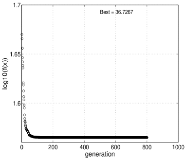
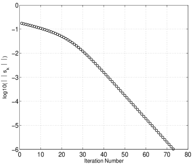
Figure 4: Convergence of the hybrid optimization method. Left: reduction of the bulk energy in the GA. Right: reduction of the step size in the quasi-Newton method

To analyze the performance of the hybrid optimization method for phase combination simulation, the bulk energy given by Eq.(16) has been monitored in the GA, and plotted in Fig.4 (left). The quasi-Newton iteration process has also been monitored. The actual update step size in the quasi-Newton method is plotted in Fig.4 (right). The trends in the two curves demonstrate how the optimization process evolves. As expected, the GA starts to converge to the global minimizer gradually, but has difficulty to locate it precisely. The quasi-Newton method starts with the output of the GA as its initial guess, and refined the global minimizer effectively.

The final estimation for the phase combination in this case is given in the right column in Fig.5: the order parameter $\epsilon$ (upper plot) and the displacement (lower plot). We observe that the entire domain is divided into two parts, one with the strain values $\epsilon\simeq 0.11$ and the other with $\epsilon\simeq-0.11$. This phase combination agrees well with the previously reported results (e.g., [13, 19, 25]). For comparison purpose, we have also provided an approximation obtained with the GA at the initial stage of the procedure (see the left column of Fig.5). Although the quality of the final solution has been refined with the quasi-Newton procedure, we note that the two parts in the distribution of $\epsilon$ are captured by the GA. Quantitative values are easily identified as being between $0.1$ to $0.15$ for one of the domains and between $-0.15$ to $-0.1$ for the other.

The second experiment aims at simulating the phase combination in a 2D SMA patch sketched in Fig.3. The size of the patch is $[-1,1]\times[-1,1]cm^{2}$ and the applied mechanical forces $f_{x}=f_{y}=3000g/\left(ms^{2}cm^{2}\right)$ are distributed evenly through the entire patch. In this case, we use $u_{x}=({\rm rand}-0.5)/5$ and $u_{y}=({\rm rand}-0.5)/5$ as the initial conditions. In this experiment, we use different node numbers for the GA and the quasi-Newton method. In the GA, there are $9$ nodes in each direction used for the discretization along the $x$ and $y$ axes. This leads to the total number of optimization parameters being $128$. The filter operation is carried out in the same way as explained for the 1D experiment, but for both $x$ and $y$ directions, and the number of nodes in each direction on the sparse grid is $6$. The GA is firstly run $1500$ generations with $120$ chromosomes in each generation. The output of the GA is then interpolated onto a denser grid with $15$ nodes in each direction, and is used as the initial guess for the quasi-Newton method. The interpolation methodology is based on the pseudospectral method with the Chebyshev collocation points, as discussed in Section 3.

The final phase combination estimated in this case are presented in Fig.6. The distribution of the order parameter $e_{2}$ is given in the upper right subplot. For comparison purpose, the estimated distribution of $e_{2}$ from the GA is presented in the upper left subplot. The final displacement distributions along the $x$ and $y$ directions are presented by the two lower subplots. Once again, the entire domain can be divided by two parts with values $e_{2}\simeq 0.11$ $e_{2}\simeq-0.11$, respectively, referred to as martensite plus and martensite minus [24, 29].

In the last experiment, we consider the same patch $[0,1]\times[0,1]cm^{2}$ with modified distributed forces $f_{y}=0,f_{x}=2000g/\left(ms^{2}cm^{2}\right)$ (with the same initial conditions as in the previous experiment). All other computational parameters are taken the same as those in the previous experiment. The numerical results are presented in Fig.7 in a way similar to already reported. In this case, the entire structure is divided into martensite plus and minus in a different way, the interface is the central vertical line due to the horizontal symmetric loading. The simulated order parameter is still close to either $0.11$ or $-0.11$ and the estimated $e_{2}$ distribution obtained with the GA can capture the essence of its final profile.

In the analysis that follows we explain why the order parameter takes values close to either $0.11$ or $-0.11$. From the Landau free energy function, it is easy to estimate the order parameter value which minimizes the local free energy by setting:

$$\frac{\delta F_{l}}{\delta e_{2}}=0.$$ (34)

For the 1D case, the order parameter should be replaced by $\epsilon$. A simple operation gives the following equation:

$$a_{2}(\Delta\theta)e_{2}-a_{4}e_{2}^{3}+a_{6}e_{2}^{5}=0,$$ (35)

which means:

$$e_{2}=\frac{a_{4}\pm\sqrt{a_{4}^{2}-4a_{6}a_{2}\Delta\theta}}{2a_{6}}.$$ (36)

Note that $e_{2}=0$ is also a solution to (35) and can be associated with the austenite phase which is unstable at the current temperature. Therefore, martensitic phases in this case are of greater interest. The temperature difference from the transformation temperature here is given as $\Delta\theta=\theta-\theta_{0}=2^{o}$, and the local minima can be estimated as: $e_{2}=\pm 0.1146.$

All three numerical experiments have demonstrated that the distributions of the order parameter are represented by a combination of two different values, $e_{2}=\pm 0.11$, which agrees well with the prediction of the above analysis.

5 Conclusions

In the present paper, phase combinations in the 1D and 2D SMA structures have been analyzed in the case of square to rectangular transformations. The phase combinations have been obtained by minimizing the bulk energy in the considered SMAs structures, subject to given temperature distribution, mechanical loadings, and boundary conditions. By combining the global and local search techniques, the developed hybrid optimization method provides a promising strategy for the solution of the associated non-convex problem.

Figure 2: Sketch of an one dimensional SMA wire under mechanical loading

Figure 3: Sketch of a two dimensional SMA patch under mechanical loading

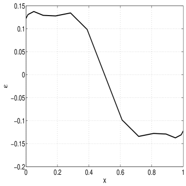
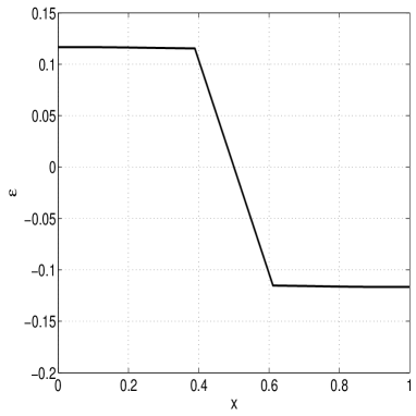
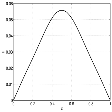
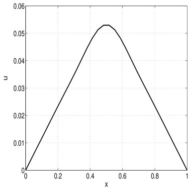
Figure 5: Mechanically induced phase combination in a SMA wire.

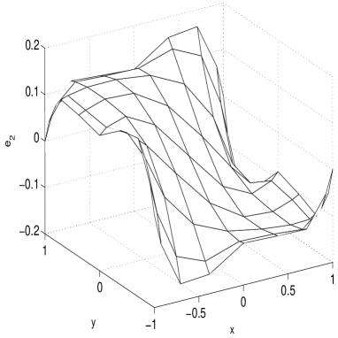
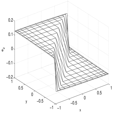
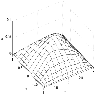
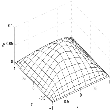
Figure 6: Phase combination in a SMA patch induced by mechanical loading along the $x$ and $y$ directions.

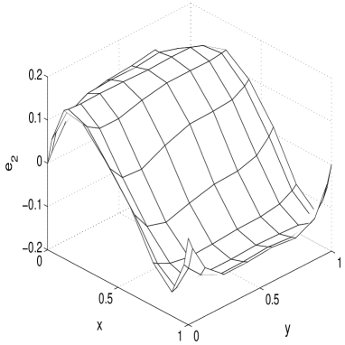
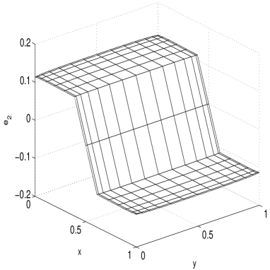
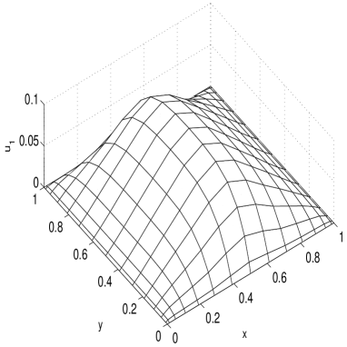
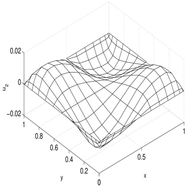
Figure 7: Phase combination in a SMA patch induced by mechanical loading along only the $x$ direction

References

- [1] R. Ahluwalia, T. Lookman, and A. Saxena, Elastic deformation of polycrystals, Phys. Rev. Lett. 91(2003), pp. 055501.
- [2] R. Ahluwalia, T. Lookman, A. Saxena, and S. R. Shenoy, Pattern formation in ferroelastic transitions, Phase Transitions, 77(5-7) (2004), pp. 457–467.
- [3] R. Ahluwalia, T. Lookman, and A. Saxena, Dynamic strain loading of cubic to tetragonal martensites, Acta Materilia, 54(2006), pp. 2109–2120.
- [4] Q. Alfio, S. Riccardo, and S. Fausto, Numerical Mathematics, Springer-Verlag, 2000.
- [5] J. M. Ball, R. D. James, Fine phase mixtures as minimizers of energy, Archive. Rat. Mech. Anal. 100(1) (1987), pp. 13–52.
- [6] J. M. Ball, and R. D. James, Proposed experimental tests of the theory of fine microstructure and the two-well problem, Philos. Trans. R. Soc. Lond., Ser. A, 338 (1992), pp. 389–450.
- [7] S. Bartels, T. Roubicek, Linear-programming approach to non-convex variational problems, Numerische Mathematik, 99(2)(2004), pp. 251–287.
- [8] V.Birman, Review of mechanics of shape memory alloys structures, Appl.Mech.Rev., 50(1997), pp. 629–645.
- [9] K. Bhattacharya, B. Li, and M. Luskin, The simply laminated microstructure in martensitic crystals that undergo a cubic to orthorhombic phase transformation, Arch. Rat. Mech. Anal. 149(1999), pp. 123–154.
- [10] C. Carstensen, Ten remarks on nonconvex minimisation for phase transition simulations. Comput. Methods Appl. Mech. engrg., 194(2005), pp. 169–193.
- [11] S. Collins, M. Luskin, and J. Riordan, Computational results for a two-dimensional model of crystalline microstructure, In.D. Kinderlehrer, R. James, M. Luskin, and J. L. Ericksen (Eds), Microstructure and Phase Transition, The IMA Volumes in Mathematics and its Applications, Vol.54, Springer, (1993), pp. 51–56.
- [12] S. H. Curnoe, and A. E. Jacobs, Time evolution of tetragonal-orthorhombic ferroelastic, Phys. Rev. B, 64(6)(2001), pp. 064101.
- [13] F. Falk, Model free energy, mechanics, and thermomechanics of shape memory alloys. Acta Metallurgica, 28(1980), pp. 1773–1780.
- [14] S. Forrest, Genetic algorithms: principles of atural selection applied to computation, Science, 261(1993), pp. 872–878.
- [15] G. Gautschi, Orthogonal polynomials and quadrature,Electronic Transaction on Numerical Algorithm, 9(1999), pp. 65–76.
- [16] D. E. Goldberg, Genetic Algorithm in Search, Optimization and Machine Learning, Addison-Wesley, 1989.
- [17] A. E. Jacobs, Landau theory of structures in tetragonal to orthorhombic ferroelastics, Phys. Rev. B, 61(10)(2000), pp. 6587–6595.
- [18] T. Lookman, S. Shenoy, D. Rasmussen, A. Saxena, and A. Bishop, Ferroelastic dynamics and strain compatibility, Phys. Rev. B, 67(2003), pp. 024114.
- [19] M. Luskin, On the computational of crystalline microstructure, Acta Numerica, 5(1996), pp. 191–256.
- [20] M. Mitchell, An Introduction to Genetic Algorithms, MIT Press, 1996.
- [21] J. M. Martinez, Practical quasi-Newton methods for solving nonlinear systems, J. Comp. App. Math., 124(2000), pp. 97–121.
- [22] P. Matus, R. V. N. Melnik, L. X. Wang, and I. Rybak, Applications of fully conservative schemes in nonlinear thermoelasticity: modelling shape memory materials, Mathematics and Computers in Simulation, 65(4-5)(2004), pp. 489–509.
- [23] R. V. N. Melnik, A. J. Roberts, and K. A. Thomas, Computing dynamics of copper-based SMA via centre manifold reduction of 3D models, Computational Materials Science, 18(3-4)(2000), pp. 255–268.
- [24] R. V. N. Melnik, A. J. Roberts, and K. A. Thomas, Coupled thermomechanical dynamics of phase transitions in shape memory alloys and related hysteresis phenomena, Mechanics Research Communications, 28(6)(2001), pp. 637–651.
- [25] M. Niezgodka, and J. Sprekels, Convergent numerical approximations of the thermomechanical phase transitions in shape memory alloys, Numerische Mathematik, 58(1991), pp. 759–778.
- [26] K. Otsuka, C. M. Wayman(editors), Shape Memory Materials, Cambridge University Press, 1998.
- [27] L. N. Trefethen, Spectral methods in Matlab, SIAM, 2000.
- [28] L. X. Wang, and R. V. N. Melnik, Dynamics of shape memory alloys patches, Materials Science and Engineering A, 378(1-2) (2004), pp. 470–474.
- [29] L. X. Wang, and R. V. N. Melnik, Thermomechanical Waves in SMA Patches under Small Mechanical Loadings, Lecture Notes in Computer Science, 3039(2004), pp. 645–653.
- [30] Y. X. Yuan, and W. Y. Sun, Theory and methods of optimization, Chinese Science Press, 1997 (in Chinese).