Multi-Antenna Cooperative Wireless Systems:
A Diversity-Multiplexing Tradeoff Perspective

Abstract

We consider a general multiple antenna network with multiple sources, multiple destinations and multiple relays in terms of the diversity-multiplexing tradeoff (DMT). We examine several subcases of this most general problem taking into account the processing capability of the relays (half-duplex or full-duplex), and the network geometry (clustered or non-clustered). We first study the multiple antenna relay channel with a full-duplex relay to understand the effect of increased degrees of freedom in the direct link. We find DMT upper bounds and investigate the achievable performance of decode-and-forward (DF), and compress-and-forward (CF) protocols. Our results suggest that while DF is DMT optimal when all terminals have one antenna each, it may not maintain its good performance when the degrees of freedom in the direct link is increased, whereas CF continues to perform optimally. We also study the multiple antenna relay channel with a half-duplex relay. We show that the half-duplex DMT behavior can significantly be different from the full-duplex case. We find that CF is DMT optimal for half-duplex relaying as well, and is the first protocol known to achieve the half-duplex relay DMT. We next study the multiple-access relay channel (MARC) DMT. Finally, we investigate a system with a single source-destination pair and multiple relays, each node with a single antenna, and show that even under the idealistic assumption of full-duplex relays and a clustered network, this virtual multi-input multi-output (MIMO) system can never fully mimic a real MIMO DMT. For cooperative systems with multiple sources and multiple destinations the same limitation remains to be in effect.

I Introduction

Next-generation wireless communication systems demand both high transmission rates and a quality-of-service guarantee. This demand directly conflicts with the properties of the wireless medium. As a result of the scatterers in the environment and mobile terminals, signal components received over different propagation paths may add destructively or constructively and cause random fluctuations in the received signal strength [1]. This phenomena, which is called fading, degrades the system performance. Multi-input multi-output (MIMO) systems introduce spatial diversity to combat fading. Additionally, taking advantage of the rich scattering environment, MIMO increases spatial multiplexing [2, 3].

User cooperation/relaying is a practical alternative to MIMO when the size of the wireless device is limited. Similar to MIMO, cooperation among different users can increase the achievable rates and decrease susceptibility to channel variations [4, 5]. In [6], the authors proposed relaying strategies that increase the system reliability. Although the capacity of the general relay channel problem has been unsolved for over thirty years [7, 8], the papers [4, 5] and [6] triggered a vast literature on cooperative wireless systems. Various relaying strategies and space-time code designs that increase diversity gains or achievable rates are studied in [9]-[36].

As opposed to the either/or approach of higher reliability or higher rate, the seminal paper [37] establishes the fundamental tradeoff between these two measures, reliability and rate, also known as the diversity-multiplexing tradeoff (DMT), for MIMO systems. At high $\mathrm{SNR}$, the measure of reliability is the diversity gain, which shows how fast the probability of error decreases with increasing $\mathrm{SNR}$. The multiplexing gain, on the other hand, describes how fast the actual rate of the system increases with $\mathrm{SNR}$. DMT is a powerful tool to evaluate the performance of different multiple antenna schemes at high $\mathrm{SNR}$; it is also a useful performance measure for cooperative/relay systems. On one hand it is easy enough to tackle, and on the other hand it is strong enough to show insightful comparisons among different relaying schemes. While the capacity of the relay channel is not known in general, it is possible to find relaying schemes that exhibit optimal DMT performance. Therefore, in this work we study cooperative/relaying systems from a DMT perspective.

In a general cooperative/relaying network with multiple antenna nodes, some of the nodes are sources, some are destinations, and some are mere relays. Finding a complete DMT characterization of the most general network seems elusive at this time, we will highlight some of the challenges in the paper. Therefore, we examine the following important subproblems of the most general network.

• Problem 1: A single source-destination system, with one relay, each node has multiple antennas,

• Problem 2: The multiple-access relay channel with multiple sources, one destination and one relay, each node has multiple antennas,

• Problem 3: A single source-destination system with multiple relays, each node has a single antenna,

• Problem 4: A multiple source-multiple destination system, each node has a single antenna.

An important constraint is the processing capability of the relay(s). We investigate cooperative/relaying systems and strategies under the full-duplex assumption, i.e. when wireless devices transmit and receive simultaneously, to highlight some of the fundamental properties and limitations. Half-duplex systems, where wireless devices cannot transmit and receive at the same time, are also of interest, as the half-duplex assumption more accurately models a practical system. Therefore, we study both full-duplex and half-duplex relays in the above network configurations.

The channel model and relative node locations have an important effect on the DMT results that we provide in this paper. In [38], we investigated Problem 3 from the diversity perspective only. We showed that in order to have maximal MIMO diversity gain, the relays should be clustered around the source and the destination evenly. In other words, half of the relays should be in close proximity to the source and the rest close to the destination so that they have a strong inter-user channel approximated as an additive white Gaussian noise (AWGN) channel. Only for this clustered case we can get maximal MIMO diversity, any other placement of relays results in lower diversity gains. Motivated by this fact, we will also study the effect of clustering on the relaying systems listed above.

I-A Related Work

Most of the literature on cooperative communications consider single antenna terminals. The DMT of relay systems were first studied in [6] and [39] for half-duplex relays. Amplify-and-forward (AF) and decode-and-forward (DF) are two of the protocols suggested in [6] for a single relay system with single antenna nodes. In both protocols, the relay listens to the source during the first half of the frame, and transmits during the second half, while the source remains silent. To overcome the losses of strict time division between the source and the relay, [6] offers incremental relaying, in which there is a 1-bit feedback from the destination to both the source and the relay, and the relay is used only when needed, i.e. only if the destination cannot decode the source during the first half of the frame. In [27], the authors do not assume feedback, but to improve the AF and DF schemes of [6] they allow the source to transmit simultaneously with the relay. This idea is also used in [39] to study the non-orthogonal amplify-and-forward (NAF) protocol in terms of DMT. Later on, a slotted AF scheme is proposed in [40], which outperforms the NAF scheme of [39] in terms of DMT. Azarian et al. also propose the dynamic decode-and-forward (DDF) protocol in [39]. In DDF the relay listens to the source until it is able to decode reliably. When this happens, the relay re-encodes the source message and sends it in the remaining portion of the frame. The authors find that DDF is optimal for low multiplexing gains but it is suboptimal when the multiplexing gain is large. This is because at high multiplexing gains, the relay needs to listen to the source longer and does not have enough time left to transmit the high rate source information. This is not an issue when the multiplexing gain is small as the relay usually understands the source message at an earlier time instant and has enough time to transmit.

MIMO relay channels are studied in terms of ergodic capacity in [41] and in terms of DMT in [42]. The latter considers the NAF protocol only, presents a lower bound on the DMT performance and designs space-time block codes. This lower bound is not tight in general and is valid only if the number of relay antennas is less than or equal to the number of source antennas.

The multiple-access relay channel (MARC) is introduced in [43, 20, 44]. In MARC, the relay helps multiple sources simultaneously to reach a common destination. The DMT for the half-duplex MARC with single antenna nodes is studied in [45, 46, 47]. In [45], the authors find that DDF is DMT optimal for low multiplexing gains; however, this protocol remains to be suboptimal for high multiplexing gains analogous to the single-source relay channel. This region, where DDF is suboptimal, is achieved by the multiple access amplify and forward (MAF) protocol [46, 47].

When multiple single antenna relays are present, the papers [9, 12, 15, 23, 27, 33, 34] show that diversity gains similar to multi-input single-output (MISO) or single-input multi-output (SIMO) systems are achievable for Rayleigh fading channels. Similarly, [6, 39, 48, 49] upper bound the system behavior by MISO or SIMO DMT if all links have Rayleigh fading. In other words, relay systems behave similar to either transmit or receive antenna arrays. Problem 4 is first analyzed in [50] in terms of achievable rates only, where the authors compare a two-source two-destination cooperative system with a $2\times 2$ MIMO and show that the former is multiplexing gain limited by 1, whereas the latter has maximum multiplexing gain of 2.

I-B Contributions

In the light of the related work described in Section I-A, we can summarize our contributions as follows:

• We study Problem 1 with full-duplex relays and compare DF and compress-and-forward (CF) [8, 20] strategies in terms of DMT for both clustered and non-clustered systems. We find that there is a fundamental difference between these two schemes. The CF strategy is DMT optimal for any number of antennas at the source, the destination or the relay, whereas DF is not.

• We also study Problem 1 with half-duplex relays. This study reveals that for half-duplex systems we can find tighter upper bounds than the full-duplex DMT upper bounds. Moreover, we show that the CF protocol achieves this half-duplex DMT bound for any number of antennas at the nodes. This is the first known result on DMT achieving half-duplex relaying protocols.

• For Problem 2 we show that the CF protocol achieves a significant portion of the half-duplex DMT upper bound for high multiplexing gains. Our results for single antenna MARC easily extend to multiple antenna terminals.

• We examine Problem 3 and Problem 4 and develop the DMT analysis to understand if the network provides any MIMO benefits. Our analysis shows that even for clustered systems with full-duplex relays, all relay systems fall short of MIMO, mainly due to multiplexing gain limitations. The same problem persists in cooperative systems with multiple source destination pairs.

Overall, our work sheds light onto high $\mathrm{SNR}$ behavior of cooperative networks as described by the DMT, and suggests optimal transmission and relaying strategies.

The paper is organized as follows. Section II describes the general system model. In Section III, we give some preliminary information that will be used frequently in the rest of the paper. In Section IV we solve the single user, single relay problem with multiple antennas for full-duplex relays, and in Section V we solve the same problem for half-duplex relays (Problem 1). Section VI introduces MARC, and suggests an achievable DMT (Problem 2). In Section VII we study two problems: the two relay system with a single source destination pair (Problem 3), and the two source two destination problem (Problem 4). Finally, in Section VIII we conclude.

II General System Model

For the most general model all the channels in the system have independent, slow, frequency non-selective, Rician fading. For Rician fading channels, the channel gain matrix is written as

$$\mathbf{H}=\sqrt{\frac{K}{K+1}}{\mathbf{H}}_{l}+\sqrt{\frac{1}{K+1}}{\mathbf{H}}_{s},$$

where $K\geq 0$, ${\mathbf{H}}_{l}$ and ${\mathbf{H}}_{s}$ denote the Rician factor, the line of sight component and the scattered component respectively. The DMT for Rician channels are studied in detail in [51]. In [51] the authors find that for finite Rician factor $K$, the channel mean does not affect the DMT behavior, and the system DMT will be equal to that of a Rayleigh fading channel with $K=0$. On the other hand in [52] the authors study the effect of $K$ on MISO and SIMO DMT when $K$ approaches infinity. They find that for large $K$, the system diversity increases linearly with $K$. Moreover, when $K$ tends to infinity, the diversity gain is infinity for all multiplexing gains up to $rank(\mathbf{H}_{l})$.

Based on the above observations, without loss of generality, in this work we assume a discrete approximation to the Rician model: If two nodes are apart more than a threshold distance $\Delta^{*}$, the line of sight component is too weak and the Rician factor $K$ can be assumed to be equal to zero. Thus the channel gain matrix is distributed as Rayleigh, and we say that the nodes are in Rayleigh zones, Fig. 1(a). On the other hand, if the inter-node distance is less than $\Delta^{*}$, the line of sight component in the received signal is strong; $K$ can be assumed to be infinity and the Rician distribution approximates a Gaussian. In this case we say that the nodes are in AWGN zones, Fig. 1(b).

For the Rayleigh zone, the channel gain matrix for MIMO terminals has independent, identically distributed (i.i.d.) zero mean complex Gaussian entries with real and imaginary parts each with variance $\sigma^{2}$. The variance $\sigma^{2}$ is proportional to $1/\Delta^{\alpha}$, where $\Delta$ denotes the internode distance, and $\alpha$ is the path loss exponent. If nodes $i$ and $j$ are in the AWGN zone, the channel gain matrix from node $i$ to $j$ has deterministic entries, all equal to $\sqrt{G_{ij}}$ and the channel gain matrix has rank 1. There is also a dead zone around the nodes, which limits the channel gain.

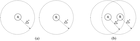
Figure 1: Two nodes A and B are in (a) Rayleigh zones, (b) AWGN zones.

Depending on the locations of the nodes, the Rayleigh or AWGN zone assumption results in two important configurations we will consider: clustered and non-clustered. For the clustered system, all the source(s) and some of the relay(s) are in the same AWGN zone, and the destination(s) and the remaining relay(s) are in another AWGN zone, but the source cluster and the destination cluster, which are more than the threshold distance $\Delta^{*}$ apart, are in their Rayleigh zones. However, for the non-clustered system, every pair of nodes in the system are in their Rayleigh zones. We do not explicitly study the systems in which some nodes are clustered and some are not in this paper, although our results can easily be applied to these cases as well.

The relay(s) can be full-duplex, that is they can transmit and receive at the same time in the same band (Sections IV, and VII), or half-duplex (Sections V and VI). The transmitters (source(s) and relay(s)) in the systems under consideration have individual power constraints $P_{i}$. All the noise vectors at the receivers (relay(s) and destination(s)) have i.i.d. complex Gaussian entries with zero mean and variance 1. Without loss of generality we assume the transmit power levels are such that the average received signal powers at the destination(s) are similar, and we define $\mathrm{SNR}$ as the common average received signal to noise ratio (except for constant multiplicative factors) at the destination. Because of this assumption, for the clustered systems we study in Section VII, the nodes in the source cluster hear the transmitters in their cluster much stronger than the transmitters in the destination cluster, and for all practical purposes we can ignore the links from the destination cluster to the nodes in the source cluster. This assumption is the same as the level set approach of [11]. For non-clustered systems each node can hear all others.

All the receivers have channel state information (CSI) about their incoming fading levels. Furthermore, the relays that perform CF have CSI about all the channels in the system. This can happen at a negligible cost by proper feedback. We will explain why we need this information when we discuss the CF protocol in detail in Section IV. The source(s) does not have instantaneous CSI. We also assume the system is delay-limited and requires constant-rate transmission. We note that under this assumption, information outage probability is still well-defined and DMT is a relevant performance metric [53]. There is also short-term average power constraint that the transmitters have to satisfy for each codeword transmitted. For more information about the effect of CSI at the transmitter(s) and variable rate transmission on DMT we refer the reader to [54].

III Preliminaries

In this section we first introduce the notation, and present some results we will use frequently in the paper.

For notational simplicity we write $f(\mathrm{SNR})\dot{=}\mathrm{SNR}^{c}$, if

$$\lim_{\mathrm{SNR}\rightarrow\infty}\frac{\log f(\mathrm{SNR})}{\log\mathrm{SNR}}=c.$$

The inequalities $\dot{\geq}$ and $\dot{\leq}$ are defined similarly. In the rest of the paper $\mathbf{I}_{i}$ denotes the identity matrix of size $i\times i$, ${\dagger}$ denotes conjugate transpose, and $|.|$ denotes the determinant operation. To clarify the variables, we would like to note that $R_{i}$ denotes the $i$th relay, whereas $R^{(.)}$ denotes transmission rates; e.g. $R^{(T)}$ will be used for target data rate.

Let $R^{(T)}(\mathrm{SNR})$ denote the transmission rate of the system and $P_{e}({\mathrm{SNR}})$ denote the probability of error. Then we define multiplexing gain $r$ and corresponding diversity $d(r)$ as

$$\lim_{\mathrm{SNR}\rightarrow\infty}\frac{R^{(T)}(\mathrm{SNR})}{\log\mathrm{SNR}} = r,$$

$$\lim_{\mathrm{SNR}\rightarrow\infty}\frac{\log P_{e}(\mathrm{SNR})}{\log\mathrm{SNR}} = -d(r).$$

The DMT of an $m\times n$ MIMO is given by $d_{mn}(r)$, the best achievable diversity, which is a piecewise-linear function connecting the points $(k,d_{mn}(k))$, where $d_{mn}(k)=(m-k)(n-k)$, $k=0,1,...,\min\{m,n\}$ [37]. Note that $d_{mn}(r)=d_{nm}(r)$.

In [37], the authors prove that the probability of error is dominated by the probability of outage. Therefore, in the rest of the paper we will consider outage probabilities only.

We know that for any random channel matrix $\mathbf{H}$ of size $n\times m$ and for any input covariance matrix $Q$ of size $m\times m$ [37],

$$\sup_{Q\geq 0,\mathrm{trace}\{Q\}\leq{m\mathrm{SNR}}}\log\left|\mathbf{I}_{n}+\mathbf{H}Q\mathbf{H}^{{\dagger}}\right|$$ (1)

$$\leq \log\left|\mathbf{I}_{n}+m\mathrm{SNR}\mathbf{H}\mathbf{H}^{{\dagger}}\right|.$$

Combined with the fact that a constant scaling in the transmit power levels do not change the DMT [37], this bound will be useful to establish DMT results.

In a general multi-terminal network, node $k$ sends information to node $l$ at rate

$$R^{(kl)}=\frac{1}{\eta}I(W_{kl};\hat{W}_{kl}),$$

where $\eta$ is the number of channel uses, $W_{kl}$ denotes the message for node $l$ at node $k$, and $\hat{W}_{kl}$ is $W_{kl}$’s estimate at node $l$. Then the maximum rate of information flow from a group of sources to a group of sinks is limited by the minimum cut [55, Theorem 14.10.1] and we cite this result below.

Proposition 1

Consider communication among $m$ nodes in a network. Let $\mathcal{C}_{i}\subset\{1,2,...,m\}$ and $\mathcal{C}_{i}^{c}$ be the complement of $\mathcal{C}_{i}$ in the set $\{1,2,...,m\}$. Also $\mathbf{X}^{(\mathcal{C}_{i})}$ and $\mathbf{X}^{(\mathcal{C}_{i}^{c})}$ denote transmitted signals from the sets $\mathcal{C}_{i}$ and $\mathcal{C}_{i}^{c}$ respectively. $\mathbf{Y}^{(\mathcal{C}_{i}^{c})}$ denotes the signals received in the set $\mathcal{C}_{i}^{c}$. For information rates $R^{(kl)}$ from node $k$ to $l$, there exists some joint probability distribution $p(x_{1},x_{2},...,x_{m})$, such that

$$\sum_{k\in\mathcal{C}_{i},l\in\mathcal{C}_{i}^{c}}R^{(kl)}\leq I_{\mathcal{C}_{i}}=I(\mathbf{X}^{(\mathcal{C}_{i})};\mathbf{Y}^{(\mathcal{C}_{i}^{c})}|\mathbf{X}^{(\mathcal{C}_{i}^{c})}),$$

for all $\mathcal{C}_{i}\subset\{1,2,...,m\}$. Thus the total rate of flow of information across cut-sets is bounded by the conditional mutual information across that cut-set.

We can use the above proposition to find DMT upper bounds. Suppose $R^{(T_{kl})}=r^{(kl)}\log\mathrm{SNR}$ denotes the target data rate from node $k$ to node $l$, and $r^{(kl)}$ is its multiplexing gain, $R^{(T_{\mathcal{C}_{i}})}=\sum_{k\in\mathcal{C}_{i},l\in\mathcal{C}_{i}^{c}}R^{(T_{kl})}$ denotes the sum target data rate across cut-set $\mathcal{C}_{i}$ and $r^{(\mathcal{C}_{i})}=\sum_{k\in\mathcal{C}_{i},l\in\mathcal{C}_{i}^{c}}r^{(kl)}$ is its sum multiplexing gain. We say the link from $k$ to $l$ is in outage if the event

$$\mathcal{E}_{kl}=\{R^{(kl)}<R^{(T_{kl})}\}$$

occurs. Furthermore, the network outage event is defined as

$$\mathcal{E}_{N}=\bigcup_{k,l\in\{1,2,...,m\},k\neq l}\mathcal{E}_{kl},$$

which means the network is in outage if any link is in outage. Minimum network outage probability is the minimum value of $P(\mathcal{E}_{N})$ over all coding schemes for the network. We name the $\mathrm{SNR}$ exponent of the minimum network outage probability as maximum network diversity, $d(\bar{r})$, where $\bar{r}$ is a vector of all $r^{(kl)}$’s. Then we have the following lemma, which says that the maximum network diversity is upper bounded by the minimum diversity over any cut.

Lemma 1

For each $\mathcal{C}_{i}\subset\{1,2,...,m\}$, define the maximum diversity order for that cut-set $d_{\mathcal{C}_{i}}(r^{(\mathcal{C}_{i})})$ as

$$d_{\mathcal{C}_{i}}(r^{(\mathcal{C}_{i})})=-\lim_{\mathrm{SNR}\rightarrow\infty}\frac{\log\min_{p(x_{1},x_{2},...,x_{m})}P(I_{\mathcal{C}_{i}}<R^{(T_{\mathcal{C}_{i}})})}{\log\mathrm{SNR}}.$$

Then the maximum network diversity $d(\bar{r})$ is upper bounded as

$$d(\bar{r})\leq\min_{i}\{d_{\mathcal{C}_{i}}(r^{(\mathcal{C}_{i})})\}.$$

Proof:

We provide the proof in Appendix A. ∎

In addition to Lemma 1, the following two results will also be useful for some of the proofs.

Lemma 2 ([56])

For two $n\times n$ positive definite matrices $A$ and $B$, if $A-B$ is positive semi-definite, then $|A|\geq|B|$.

Lemma 3

For two real numbers $x,y>0$, $xy/(x+y)<c$, where $c$ is a non-negative real number, implies $x<2c$, or $y<2c$. Therefore, for two non-negative random variables $X$ and $Y$, $P\left({XY}/(X+Y)<c\right)\leq P(X<2c)+P(Y<2c)$.

The proof follows from simple arithmetic operations, which we omit here.

IV Multiple Antenna Nodes, Single Full-Duplex Relay

The general multiple antenna, multiple source, destination, relay network includes the multiple antenna relay channel consisting of a single source, destination and relay, as a special case. Any attempt to understand the most general network requires us to investigate the multiple antenna relay channel in more detail. Therefore, in this section we study Problem 1, in which the source, the destination and the relay has $m$, $n$ and $k$ antennas respectively. This is shown in Fig. 2. As clustering has a significant effect on the DMT performance of the network, we will look into the non-clustered and clustered cases and examine the DF and CF protocols. In this section the relay is full-duplex, whereas in Section V, the relay will be half-duplex.

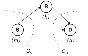
Figure 2: System model for Problem 1, the single relay system. The source, the destination and the relay have $m$, $n$ and $k$ antennas respectively.

IV-A Non-Clustered

Denoting the source and relay transmitted signals as $\mathbf{X}_{S}$ and $\mathbf{X}_{R}$, when the system is non-clustered, the received signals at the relay and at the destination are

$$\mathbf{Y}_{R} = \mathbf{H}_{SR}\mathbf{X}_{S}+\mathbf{Z}_{R}$$ (2)

$$\mathbf{Y}_{D} = \mathbf{H}_{SD}\mathbf{X}_{S}+\mathbf{H}_{RD}\mathbf{X}_{R}+\mathbf{Z}_{D},$$ (3)

where $\mathbf{Z}_{R}$ and $\mathbf{Z}_{D}$ are the independent complex Gaussian noise vectors at the corresponding node. $\mathbf{H}_{SR}$, $\mathbf{H}_{SD}$ and $\mathbf{H}_{RD}$ are the $k\times m$, $n\times m$ and $n\times k$ channel gain matrices between the source and the relay, the source and the destination, and the relay and the destination respectively.

Theorem 1

The optimal DMT for the non-clustered system of Fig. 2, $d(r)$, is equal to

$$d(r)=\min\{d_{m(n+k)}(r),d_{(m+k)n}(r)\},$$

and the CF protocol achieves this optimal DMT for any $m$, $n$ and $k$.

Proof:

1) Upper Bound: The instantaneous cut-set mutual information expressions for cut-sets $\mathcal{C}_{S}$ and $\mathcal{C}_{D}$ are

$$I_{\mathcal{C}_{S}} = I(\mathbf{X}_{S};\mathbf{Y}_{R}\mathbf{Y}_{D}|\mathbf{X}_{R})$$ (4)

$$I_{\mathcal{C}_{D}} = I(\mathbf{X}_{S}\mathbf{X}_{R};\mathbf{Y}_{D}).$$ (5)

To maximize these mutual information expressions we need to choose $\mathbf{X}_{S}$ and $\mathbf{X}_{R}$ complex Gaussian with zero mean and covariance matrices having trace constraints $P_{S}$ and $P_{R}$ respectively, where $P_{S}$ and $P_{R}$ denote the average power constraints each node has [57]. Moreover, the covariance matrix of $\mathbf{X}_{S}$ and $\mathbf{X}_{R}$ should be chosen appropriately to maximize $I_{\mathcal{C}_{D}}$. Then using (1) to upper bound $I_{\mathcal{C}_{S}}$ with $I_{\mathcal{C}_{S}}^{\prime}$ and $I_{\mathcal{C}_{D}}$ with $I_{\mathcal{C}_{D}}^{\prime}$ we can write

$$I_{\mathcal{C}_{S}} \leq I_{\mathcal{C}_{S}}^{\prime}=\log K_{S,RD}^{\prime}$$ (6)

$$I_{\mathcal{C}_{D}} \leq I_{\mathcal{C}_{D}}^{\prime}=\log K_{SR,D},$$ (7)

where

$$K_{S,RD}^{\prime} \triangleq \left|\mathbf{I}_{k+n}+\mathbf{H}_{S,RD}\mathbf{H}_{S,RD}^{{\dagger}}P_{S}\right|$$ (8)

$$K_{SR,D} \triangleq \left|\mathbf{I}_{n}+\mathbf{H}_{SR,D}\mathbf{H}_{SR,D}^{{\dagger}}(P_{S}+P_{R})\right|,$$ (9)

with

$$\mathbf{H}_{S,RD}=\left[\begin{array}[]{c}\mathbf{H}_{SR}\\ \mathbf{H}_{SD}\\ \end{array}\right],~{}~{}\mathbf{H}_{SR,D}=\left[\begin{array}[]{cc}\mathbf{H}_{SD}&\mathbf{H}_{RD}\\ \end{array}\right].$$ (13)

The above bounds suggest that the CSI at the relay does not improve the DMT performance under short term power constraint and constant rate operation. The best strategy for the relay is to employ beamforming among its antennas. For an $m$ antenna MIMO, with total transmit power $P$, the beamforming gain can at most be $mP$ [37], which results in the same DMT as using power $P$. Therefore, CSI at the relay with no power allocation over time does not improve the DMT, it has the same the DMT when only receiver CSI is present.

Note that $P(I_{\mathcal{C}_{i}}^{\prime})\dot{=}\mathrm{SNR}^{-d_{\mathcal{C}_{i}}^{\prime}(r)}$, $i=S,D$, with $d_{\mathcal{C}_{S}}^{\prime}(r)=d_{m(n+k)}(r)$ and $d_{\mathcal{C}_{D}}^{\prime}(r)=d_{(m+k)n}(r)$. Then using Lemma 1, one can easily upper bound the system DMT by

$$d(r)\leq\min\{d_{m(n+k)}(r),d_{(m+k)n}(r)\},$$

for a target data rate $R^{(T)}=r\log\mathrm{SNR}$.

2) Achievability: To prove the DMT upper bound of Theorem 1 is achievable, we assume the relay does full-duplex CF as we explain below. We assume the source, and the relay perform block Markov superposition coding, and the destination does backward decoding [20, 58, 59]. The encoding is carried over $B$ blocks, over which the fading remains fixed. In the CF protocol the relay performs Wyner-Ziv type compression with side information taken as the destination’s received signal. For this operation the relay needs to know all the channel gains in the system.

For the CF protocol, as suggested in [8] and [20], the relay’s compression rate has to satisfy

$$I(\hat{\mathbf{Y}}_{R};\mathbf{Y}_{R}|\mathbf{X}_{R}\mathbf{Y}_{D})\leq I(\mathbf{X}_{R};\mathbf{Y}_{D}),$$ (14)

in order to forward $\hat{\mathbf{Y}}_{R}$ reliably to the destination. Here $\hat{\mathbf{Y}}_{R}$ denotes the compressed signal at the relay. The destination can recover the source message reliably if the transmission rate $R^{(T)}=r\log\mathrm{SNR}$ of the source is less than the instantaneous mutual information $R^{(CF)}$

$$R^{(CF)}=I(\mathbf{X}_{S};\hat{\mathbf{Y}}_{R}\mathbf{Y}_{D}|\mathbf{X}_{R}).$$ (15)

We assume $\mathbf{X}_{S}$ and $\mathbf{X}_{R}$ are chosen independently, and have covariance matrices $\mathbf{I}_{m}P_{S}/m$ and $\mathbf{I}_{k}P_{R}/k$ respectively. Also $\hat{\mathbf{Y}}_{R}=\mathbf{Y}_{R}+\hat{\mathbf{Z}}_{R}$, where $\hat{\mathbf{Z}}_{R}$ is a length $k$ vector with complex Gaussian random entries with zero mean. $\hat{\mathbf{Z}}_{R}$ has covariance matrix $\hat{N}_{R}\mathbf{I}_{k}$, and its entries are independent from all other random variables. We define

$$L_{S,D} \triangleq \left|\mathbf{H}_{SD}\mathbf{H}_{SD}^{\dagger}\frac{P_{S}}{m}+\mathbf{I}_{n}\right|$$ (16)

$$L_{SR,D} \triangleq \left|\mathbf{H}_{SD}\mathbf{H}_{SD}^{{\dagger}}\frac{P_{S}}{m}+\mathbf{H}_{RD}\mathbf{H}_{RD}^{{\dagger}}\frac{P_{R}}{k}+\mathbf{I}_{n}\right|,$$ (17)

$$L_{S,RD} \triangleq \left|\mathbf{H}_{S,RD}\mathbf{H}_{S,RD}^{{\dagger}}\frac{P_{S}}{m}+\left[\begin{array}[]{cc}(\hat{N}_{R}+1)\mathbf{I}_{k}&\mathbf{0}\\ \mathbf{0}&\mathbf{I}_{n}\end{array}\right]\right|.$$ (20)

$$L_{S,RD}^{\prime} \triangleq \left|{\mathbf{H}_{S,RD}}\mathbf{H}_{S,RD}^{{\dagger}}\frac{P_{S}}{m}+\mathbf{I}_{k+n}\right|$$ (21)

Then we have

$$I(\hat{\mathbf{Y}}_{R};\mathbf{Y}_{R}|\mathbf{X}_{R}\mathbf{Y}_{D}) = \log\frac{L_{S,RD}}{L_{S,D}\hat{N}_{R}^{k}}$$

$$I(\mathbf{X}_{R};\mathbf{Y}_{D}) = \log\frac{L_{SR,D}}{L_{S,D}}.$$

To satisfy the compression rate constraint in (14), using the CSI available to it, the relay ensures that the compression noise variance $\hat{N}_{R}$ satisfies $\hat{N}_{R}=\sqrt[k]{L_{S,RD}/L_{SR,D}}$. Note that both sides of this equation are functions of $\hat{N}_{R}$. Then

$$R^{(CF)} = I(\mathbf{X}_{S};\hat{\mathbf{Y}}_{R}\mathbf{Y}_{D}|\mathbf{X}_{R})$$ (22)

$$= \log\frac{L_{S,RD}}{\left(\sqrt[k]{\frac{L_{S,RD}}{L_{SR,D}}}+1\right)^{k}}$$

$$= \log\left(\frac{\sqrt[k]{L_{S,RD}}\sqrt[k]{L_{SR,D}}}{\sqrt[k]{L_{S,RD}}+\sqrt[k]{L_{SR,D}}}\right)^{k}.$$

To prove the DMT of (22) we need to find how probability of error decays with increasing $\mathrm{SNR}$ when the target rate increases as $R^{(T)}=r\log\mathrm{SNR}$. As the error events are dominated by outage events, we use the following bound on the probability of outage

$$P(\mbox{outage at D})$$ (23)

$$= P\left(I(\mathbf{X}_{S};\hat{\mathbf{Y}}_{R}\mathbf{Y}_{D}|\mathbf{X}_{R})<r\log\mathrm{SNR}\right)$$

$$= P\left(\frac{\sqrt[k]{L_{S,RD}}\sqrt[k]{L_{SR,D}}}{\sqrt[k]{L_{S,RD}}+\sqrt[k]{L_{SR,D}}}<\mathrm{SNR}^{\frac{r}{k}}\right)$$ (24)

$$\overset{(a)}{\leq} P\left(\frac{\sqrt[k]{L_{S,RD}^{\prime}}\sqrt[k]{L_{SR,D}}}{\sqrt[k]{L_{S,RD}^{\prime}}+\sqrt[k]{L_{SR,D}}}<\mathrm{SNR}^{\frac{r}{k}}\right)$$ (27)

$$\overset{(b)}{\leq} P\left(\sqrt[k]{L_{S,RD}^{\prime}}<2\mathrm{SNR}^{\frac{r}{k}}\right)$$

$${+}\>P\left(\sqrt[k]{L_{SR,D}}<2\mathrm{SNR}^{\frac{r}{k}}\right)$$

$$= P\left(L_{S,RD}^{\prime}<2^{k}\mathrm{SNR}^{r}\right)$$

$${+}\>P\left(L_{SR,D}<2^{k}\mathrm{SNR}^{r}\right)$$

$$\overset{(c)}{\dot{=}} {\mathrm{SNR}^{-d_{\mathcal{C}_{S}}^{\prime}(r)}}+{\mathrm{SNR}^{-d_{\mathcal{C}_{D}}^{\prime}(r)}}$$

$${=} {\mathrm{SNR}^{-d_{m(n+k)}(r)}}+{\mathrm{SNR}^{-d_{(m+k)n}(r)}}.$$

where for $(a)$ we first used Lemma 2 to show $L_{S,RD}\geq L_{S,RD}^{\prime}$ and the fact that the ratio $xy/(x+y)$ is monotone decreasing with decreasing $x$ for $x,y>0$, $(b)$ follows from Lemma 3, and $(c)$ follows because $\log L_{S,RD}^{\prime}$ and $\log L_{SR,D}$ are same as the cut-set mutual information expressions $I_{\mathcal{C}_{S}}$ and $I_{\mathcal{C}_{D}}$ except a constant scaling factor of $\mathrm{SNR}$, and a constant scaling in $\mathrm{SNR}$ in the probability expression does not change the diversity gain. We conclude that the system DMT $d_{CF}(r)\geq\min\{d_{m(n+k)}(r),d_{(m+k)n}(r)\}$. This result when combined with the upper bound results in

$$d_{CF}(r)=\min\{d_{m(n+k)}(r),d_{(m+k)n}(r).\}$$

∎

As an alternative to the CF protocol, the relay can use the DF protocol. When the source, the destination and the relay all have a single antenna each, it is easy to show that the DF protocol also achieves the DMT upper bound, which is equal to $d_{12}(r)$. The following theorem derives the DMT of the DF protocol for arbitrary $m$, $n$ and $k$ and shows that the optimality of DF does not necessarily hold for all $m$, $n$ and $k$.

Theorem 2

For the system in Fig. 2, DF achieves the DMT

$$d_{DF}(r)=\left\{\begin{array}[]{l}\min\{d_{(m+k)n}(r),d_{mn}(r)+d_{mk}(r)\}\\ \mbox{~{}~{}~{}~{}~{}~{}~{}~{}~{}~{}~{}~{}~{}~{}~{}~{}~{}if~{}}0\leq r\leq\min\{m,n,k\}\\ d_{mn}(r)\\ \mbox{~{}~{}~{}~{}~{}if~{}}\min\{m,n,k\}<r\leq\min\{m,n\}\\ \end{array}\right..$$ (33)

Proof:

We provide the proof in Appendix B. ∎

We next consider examples for the DF DMT performance and compare with Theorem 1. If $m$ or $n$ (or both) is equal to 1, we find that DF meets the bound in Theorem 1 and is optimal irrespective of the value of $k$. Similarly we can show that for cases such as $(m,n,k)=(3,2,2)$ or $(m,n,k)=(4,2,3)$, as $d_{(m+k)n}(r)<d_{mn}(r)+d_{mk}(r)$ for all $r$, DF is optimal. A general necessary condition for DF to be optimal for all multiplexing gains is $m\geq n$. If $m<n$, then $d_{mn}(r)+d_{mk}(r)\leq d_{m(n+k)}(r)<d_{(m+k)n}$, and DF will be suboptimal.

Whenever $\min\{m,n,k\}=k$, the degrees of freedom in the direct link is larger than the degrees of freedom in the source to relay link, that is $\min\{m,n\}\geq\min\{m,k\}$. For multiplexing gains in the range $\min\{m,n,k\}<r\leq\min\{m,n\}$, the relay can never help and the system has the direct link DMT $d_{mn}(r)$. Therefore, DF loses its optimality. For example, if $(m,n,k)=(3,2,1)$, then DF is optimal only for multiplexing gains up to $1/2$, but for $1/2\leq r\leq 2$, DF is suboptimal. In particular, DF does not improve upon $d_{32}(r)$ in the range $1\leq r\leq 2$.

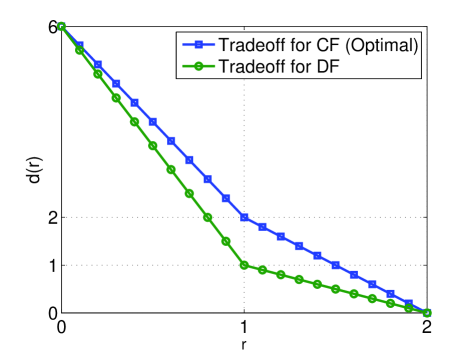
Figure 3: The source has 2, the destination has 2, and the relay has 1 antenna, $(m,n,k)=(2,2,1)$. The network is non-clustered.

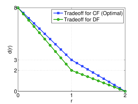
Figure 4: The source has 2, the destination has 2, and the relay has 2 antennas, $(m,n,k)=(2,2,2)$. The network is non-clustered.

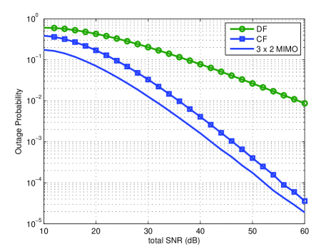
Figure 5: Outage probability versus total $\mathrm{SNR}$ for the non-clustered multiple-antenna, single full-duplex relay system, $(m,n,k)=(2,2,1)$, $r=1.5$.

Fig. 3 shows the CF and DF DMT for $(m,n,k)=(2,2,1)$, and Fig. 4 shows the CF and DF DMT for $(m,n,k)=(2,2,2)$. When we compare the figures, we see that the CF protocol is always DMT optimal, but the DF protocol can still be suboptimal even when the source to relay link has the same degrees of freedom as the link from the source to the destination. The suboptimal behavior of DF arises because the outage event when the relay cannot decode can dominate for general $m,n$ and $k$. In addition to this, for multiplexing gains larger than $\min\{m,n,k\}$, the relay never participates in the communication because it is degrees of freedom limited and cannot decode large multiplexing gain signals. For this region, we observe the direct link behavior. We conclude that soft information transmission, as in the CF protocol, is necessary at the relay not to lose diversity or multiplexing gains.

Fig. 5 shows the outage probability versus total $\mathrm{SNR}$ for DF and CF protocols for $(m,n,k)=(2,2,1)$, $R^{(T)}=r\log(P_{S}+P_{R})$, $r=1.5$. The channel gain matrices $\mathbf{H}_{SR}$, $\mathbf{H}_{SD}$ and $\mathbf{H}_{RD}$ have i.i.d. complex Gaussian entries, with real and imaginary parts zero mean and variance $1/2$ each. We have $P_{S}=2P_{R}$. The figure also includes the $3\times 2$ MIMO for comparison. We assume the total power constraint is the same for both the MIMO and relay systems. In the MIMO system the antennas share the total power equally and send uncorrelated signals. We observe that while DF achieves $d=0.5$, CF achieves $d=1$ and performs similar to $3\times 2$ MIMO as predicted by Theorem 1.

The above analysis also reveals that CF and DF protocols do not always behave similar, unlike the single antenna relay system. The degrees of freedom available also has an effect on relaying strategies.

IV-B Clustered

Clustering can sometimes improve the system performance, since it eliminates fading between some of the users. We will observe an example of this in Section VII, when there are multiple relays. Therefore, in this subsection we study the DMT behavior of a single relay system, when the relay is clustered with the source. The analysis presented in this subsection can easily be modified if relay is clustered with the destination. The system input and output signals are same as (2) and (3) but for the clustered case all the entries of $\mathbf{H}_{SR}$ are equal to $\sqrt{G}$.

Theorem 3

For the system in Fig. 2 when the relay is clustered with the source, the CF protocol is optimal from the DMT perspective for all $(m,n,k)$.

We omit the proof, as the achievability follows the same lines as in Theorem 1, and results in the same outage probability expression in (IV-A), which is equal to the upper bound.

We next compute the DMT of the clustered system explicitly for $m=1,2$, arbitrary $n$ and $k$. We conjecture the same form holds for arbitrary $m$ as well.

Theorem 4

For the clustered system of Fig. 2, for $(m,n,k)$, $m=1,2$, the DMT is given by

$$d(r)=\left\{\begin{array}[]{l}d_{(m+k)n}(r)\mbox{~{}~{}~{}~{}~{}~{}~{}~{}~{}~{}~{}~{}~{}~{}~{}~{}~{}~{}~{}~{}~{}~{}~{}~{}~{}~{}~{}if~{}}0\leq r<1\\ \min\{d_{m(n+1)}(r),d_{(m+k)n}(r)\}\\ \mbox{~{}~{}~{}~{}~{}~{}~{}~{}~{}~{}~{}~{}~{}~{}~{}~{}~{}~{}~{}~{}~{}~{}~{}~{}~{}~{}~{}~{}~{}~{}if~{}}1\leq r\leq\min\{m,n\}\\ \end{array}\right..$$

Proof:

We provide the proof in Appendix C. ∎

For the clustered case, for any $m$ or $k$, $\mathbf{H}_{SR}$ has rank 1, hence we have the following conjecture.

Conjecture 1

Theorem 4 is true for arbitrary $(m,n,k)$.

We observe that if $m=2$, although the source and the relay both have multiple antennas, as the channel gain matrix in between is AWGN and has rank 1, it can only support multiplexing gains up to 1. This is because having multiple antennas at the transmitter and/or the receiver in an AWGN channel only introduces power gain. Therefore, $I_{\mathcal{C}_{S}}$, the mutual information across cut-set $\mathcal{C}_{S}$, never results in outage for multiplexing gains up to 1. For multiplexing gains $r\geq 1$, this cut-set results in a DMT of $d_{2(n+1)}(r)$, even though the relay has $k$ antennas. The next theorem is a counterpart of Theorem 2 for the clustered case.

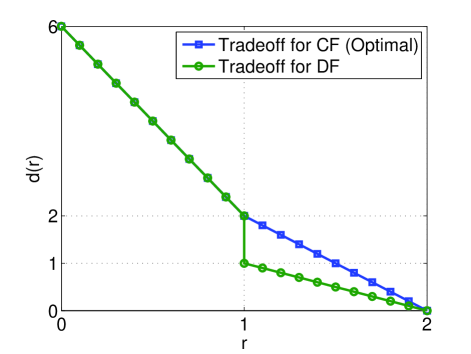
Figure 6: The source has 2, the destination has 2, and the relay has 1 antenna, $(m,n,k)=(2,2,1)$. The relay is clustered with the source.

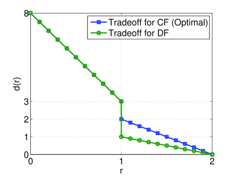
Figure 7: The source has 2, the destination has 2, and the relay has 2 antennas, $(m,n,k)=(2,2,2)$. The relay is clustered with the source.

Theorem 5

For the system in Fig. 2, when the relay is clustered with the source, the DF protocol achieves the DMT

$$d_{DF}(r) = \left\{\begin{array}[]{lll}d_{(m+k)n}(r)&\mbox{if}&0\leq r<1\\ d_{mn}(r)&\mbox{if}&1<r\leq\min\{m,n\}\\ \end{array}\right..$$

Proof:

The outage probability for DF is the same as (B), in the non-clustered case of Appendix B. If $0\leq r<1$, then the probability that the relay is in outage is 0. On the other hand, if $1\leq r\leq\min\{m,n\}$, the probability that the relay can decode is 0, since the source-relay channel can only support multiplexing gains up to 1. ∎

We have seen in Section IV-A that DF is in general suboptimal for non-clustered multi-antenna relay channel. However, once we cluster the relay with the source, there are no more outages in the source-relay channel for multiplexing gains up to 1, and the DF performance improves in this range. However, even with clustering DF does not necessarily meet the DMT upper bound for arbitrary $(m,n,k)$.

Fig. 6 compares the clustered CF and DF DMT for $(m,n,k)=(2,2,1)$, and Fig. 7 for $(m,n,k)=(2,2,2)$. Comparing with the upper bound, we can see that clustering improves the DF performance in the range $0\leq r\leq 1$, where DF achieves the upper bound. However, for multiplexing gains larger than 1, DF is still suboptimal. In fact, in this range the relay can never decode the source even though they are clustered and hence cannot improve the direct link performance. Although clustering improves the DF performance for low multiplexing gains, it is not beneficial for multiple antenna scenarios in terms of DMT, it can in fact decrease the optimal diversity gain. This is because when two nodes have multiple antennas, clustering decreases the degrees of freedom in between. This can also be observed comparing Theorem 4 and Theorem 1, as well as the optimal strategies in Fig. 7 with Fig. 4. We will also study the effects of clustering in single antenna multiple relay scenarios in Section VII.

V Multiple Antenna Nodes, Single Half-Duplex Relay

In the previous section, we studied the relay channel when the relay is full-duplex. Although this is an ideal assumption about the relay’s physical capabilities, it helps us understand the fundamental differences between the DF and CF protocols. In this section we assume a half-duplex, non-clustered relay to study how this affects the DMT behavior of the relay channel.

In half-duplex operation a state variable $Q$, which takes the value $q_{1}$ if the relay is listening, or $q_{2}$ if the relay is transmitting, controls the relay operation. For a more general treatment that considers three different states depending on whether the relay is in sleep, listen or talk states see [60]. Our results in this section would also be applicable for this case as well.

Depending on how the state $Q$ is designed, half-duplex protocols can be random or fixed. In fixed protocols, the state does not convey additional information to the destination via the state random variable $Q$, whereas in random protocols the relay breaks its transmission and reception intervals into small blocks to send extra information through the state. This is equivalent to considering the random binary state as a channel input and designing code books to convey information through $Q$.

Another categorization based on the state variable $Q$ is dynamic versus static. If the state is controlled based on channel realizations, we have a dynamic protocol. On the other hand, if $Q$ does not depend on CSI, the protocol is called static. Note that fixed protocols are included in random ones, and static protocols in dynamic ones. The most commonly used relaying protocols are fixed and static, and of the form shown in Fig. 8. The DDF protocol of [39] is an example to a fixed, dynamic protocol.

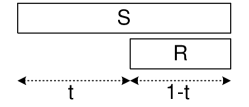
Figure 8: A fixed and static half-duplex relaying protocol, where the relay listens for $t$ fraction of time, transmits for $(1-t)$ fraction, where $t$ is a constant.

For the multiple antenna half-duplex relay channel, using Lemma 1 directly, results in the full-duplex bound, which is not tight for half-duplex operation. Therefore, we first state the following lemma to provide a half-duplex DMT upper bound for random, static protocols. The lemma also suggests that sending information through the state does not improve DMT. Lemma 4 can be modified for random, dynamic state protocols as well.

Lemma 4

For the multiple antenna half-duplex relay channel, the half-duplex DMT upper bound for random, static state protocols is equal to

$$d(r)\leq\max_{p(q)}\min\{d_{\mathcal{C}_{S}}(r,p(q)),d_{\mathcal{C}_{D}}(r,p(q))\},$$ (35)

where

$$d_{\mathcal{C}_{i}}(r,p(q))$$ (36)

$$= -\lim_{\mathrm{SNR}\rightarrow\infty}\frac{\log\min_{p(x_{S},x_{R}|q)}P(I_{\mathcal{C}_{i}}<R^{(T)})}{\log\mathrm{SNR}},$$

$i=S,D$.

Proof:

We provide the proof in Appendix D. ∎

Our next theorem and corollary provide the first half-duplex DMT achieving relaying protocol in the literature.

Theorem 6

For the random, dynamic state, half-duplex relay channel with $m$ antenna source, $k$ antenna relay and $n$ antenna destination, the CF protocol is DMT optimal.

Corollary 1

For $(m,n,k)=(1,1,1)$, the half-duplex DMT upper bound is equal to the full-duplex DMT, $2(1-r)$. Therefore, CF is a DMT optimal half-duplex protocol for the single antenna relay channel.

Proof:

[Theorem 6] First, we prove that CF is optimal among static protocols and then show that the same proof follows for dynamic protocols as well.

At state $q_{1}$, the received signals at the relay and the destination are

$$\mathbf{Y}_{R,1} = \mathbf{H}_{SR}\mathbf{X}_{S,1}+\mathbf{Z}_{R,1}$$

$$\mathbf{Y}_{D,1} = \mathbf{H}_{SD}\mathbf{X}_{S,1}+\mathbf{Z}_{D,1}$$

and at state $q_{2}$, the received signal at the destination is given as

$$\mathbf{Y}_{D,2} = \mathbf{H}_{SD}\mathbf{X}_{S,2}+\mathbf{H}_{RD}\mathbf{X}_{R,2}+\mathbf{Z}_{D,2}.$$

Here $\mathbf{X}_{S,l}$, and $\mathbf{X}_{R,l}$ are of size $m$, and $k$ column vectors respectively and denote transmitted signal vectors at node $S$, and $R$ at state $q_{l}$, $l=1,2$. Similarly $\mathbf{Y}_{R,l}$ and $\mathbf{Y}_{D,l}$ are the received signal vectors of size $k$ and $n$.

We first find an upper bound to the DMT using Lemma 4. Without loss of generality we use a fixed state static protocol as shown in Fig. 8. This is justified by the proof of Lemma 4, which states that fixed and random protocols have the same DMT upper bound. For the half-duplex relay channel using the cut-set $\mathcal{C}_{S}$ around the source and $\mathcal{C}_{D}$ around the destination as shown in Fig. 2, we have [19]

$$I_{\mathcal{C}_{S}}(t) = tI(\mathbf{X}_{S};\mathbf{Y}_{R}\mathbf{Y}_{D}|q_{1})$$ (37)

$${+}\>(1-t)I(\mathbf{X}_{S};\mathbf{Y}_{D}|\mathbf{X}_{R},q_{2})$$

$$I_{\mathcal{C}_{D}}(t) = tI(\mathbf{X}_{S};\mathbf{Y}_{D}|q_{1})$$ (38)

$${+}\>(1-t)I(\mathbf{X}_{S}\mathbf{X}_{R};\mathbf{Y}_{D}|q_{2}).$$

We define

$$K_{S,D} \triangleq \left|\mathbf{H}_{SD}\mathbf{H}_{SD}^{\dagger}P_{S}+\mathbf{I}_{n}\right|.$$ (39)

Then we can upper bound $I_{\mathcal{C}_{S}}(t)$ and $I_{\mathcal{C}_{D}}(t)$ with $I_{\mathcal{C}_{S}}^{\prime}(t)$ and $I_{\mathcal{C}_{D}}^{\prime}(t)$ as

$$I_{\mathcal{C}_{S}}(t)\leq I_{\mathcal{C}_{S}}^{\prime}(t)=t\log K_{S,RD}^{\prime}+(1-t)\log K_{S,D}$$ (40)

$$I_{\mathcal{C}_{D}}(t)\leq I_{\mathcal{C}_{D}}^{\prime}(t)=t\log K_{S,D}+(1-t)\log K_{SR,D}$$ (41)

where $K_{S,RD}^{\prime}$ and $K_{SR,D}$ are defined in (8) and (9).

For a target data rate $R^{(T)}=r\log\mathrm{SNR}$, and for a fixed $t$, if $P(I_{\mathcal{C}_{i}}^{\prime}(t)<R^{(T)})\dot{=}\mathrm{SNR}^{-d_{\mathcal{C}_{i}}^{\prime}(r,t)}$, $i=S,D$, then $d_{\mathcal{C}_{i}}(r,t)$ of Lemma 4 satisfies $d_{\mathcal{C}_{i}}(r,t)\leq d_{\mathcal{C}_{i}}^{\prime}(r,t),$ where we denoted $d_{\mathcal{C}_{i}}(r,p(q))$ with $d_{\mathcal{C}_{i}}(r,t)$ with an abuse of notation. Therefore, the best achievable diversity for the half-duplex relay channel for fixed $t$ satisfies

$$d(r,t)\leq\min\{d_{\mathcal{C}_{S}}^{\prime}(r,t),d_{\mathcal{C}_{D}}^{\prime}(r,t)\}.$$ (42)

Optimizing over $t$ we find an upper bound on the static multiple antenna half-duplex relay channel DMT as

$$d(r)\leq\max_{t}\min\{d_{\mathcal{C}_{S}}^{\prime}(r,t),d_{\mathcal{C}_{D}}^{\prime}(r,t)\}.$$ (43)

Appendix E shows that half-duplex CF achieves the upper bound in (43). For dynamic protocols, the DMT upper bound will change because of the CSI available at the relay. Appendix E also shows that if CF is allowed dynamic operation, it achieves the dynamic DMT upper bound as well. ∎

V-A Static Half-Duplex DMT Computation

In general it is hard to compute the exact DMT of Theorem 6. In particular for static protocols, to find $d_{\mathcal{C}_{S}}^{\prime}(r,t)$ and $d_{\mathcal{C}_{D}}^{\prime}(r,t)$ for general $m$, $n$ and $k$ we need to calculate the joint eigenvalue distribution of two correlated Hermitian matrices, $\mathbf{H}_{SD}\mathbf{H}_{SD}^{\dagger}$ and $\mathbf{H}_{S,RD}\mathbf{H}_{S,RD}^{\dagger}$ or $\mathbf{H}_{SD}\mathbf{H}_{SD}^{\dagger}$ and $\mathbf{H}_{SR,D}\mathbf{H}_{SR,D}^{\dagger}$. However, when $m=1$, both $\mathbf{H}_{SD}\mathbf{H}_{SD}^{\dagger}$ and $\mathbf{H}_{S,RD}\mathbf{H}_{S,RD}^{\dagger}$ reduce to vectors and it becomes easier to find $d_{\mathcal{C}_{S}}^{\prime}(r,t)$. Similarly, when $n=1$, $\mathbf{H}_{SD}\mathbf{H}_{SD}^{\dagger}$ and $\mathbf{H}_{SR,D}\mathbf{H}_{SR,D}^{\dagger}$ are vectors, and $d_{\mathcal{C}_{D}}^{\prime}(r,t)$ can be found.

An explicit form for $d_{\mathcal{C}_{S}}^{\prime}(r,t)$ is given in the following theorem.

Theorem 7

For $m=1$, $d_{\mathcal{C}_{S}}^{\prime}(r,t)$ is given as

$$d_{\mathcal{C}_{S}}^{\prime}(r,t)=\left\{\begin{array}[]{lll}n+k-k\frac{r}{t}&\mbox{if}&r\leq t,\mbox{~{}and~{}}t\leq\frac{k}{n+k}\vspace{0.15 cm}\\ n\left(\frac{1-r}{1-t}\right)&\mbox{if}&r\geq t,\mbox{~{}and~{}}t\leq\frac{k}{n+k}\vspace{0.15 cm}\\ (n+k)(1-r)&\mbox{if}&t\geq\frac{k}{n+k}\end{array}\right..$$

For $n=1$ and for arbitrary $m$ and $k$, $d_{\mathcal{C}_{D}}^{\prime}(r,t)$ has the same expression as $d_{\mathcal{C}_{S}}^{\prime}(r,t)$ if $n$ and $t$ are replaced with $m$ and $(1-t)$ in the above expressions.

Proof:

The proof follows the ideas presented in [37, 39], and is provided in Appendix F. ∎

Although we do not have an explicit expression for $d_{\mathcal{C}_{S}}^{\prime}(r,t)$ or $d_{\mathcal{C}_{D}}^{\prime}(r,t)$ for general $(m,n,k)$, we can comment on some special cases and get insights about multiple antenna, half-duplex behavior. First we observe that $d_{\mathcal{C}_{S}}^{\prime}(r,t)$ and $d_{\mathcal{C}_{D}}^{\prime}(r,t)$ depend on the choice of $t$, and the upper bound of (43) is not always equal to the full-duplex bound. As an example consider $(m,n,k)=(1,1,2)$, for which $d_{\mathcal{C}_{S}}^{\prime}(r,t)$ is shown in Fig. 9. To achieve the full-duplex bound for all $r$, $d_{\mathcal{C}_{S}}^{\prime}(r,t)$ needs to have $t\geq 2/3$, whereas $d_{\mathcal{C}_{D}}^{\prime}(r,t)$ needs $t\leq 1/3$. As both cannot be satisfied simultaneously, $d(r,t)$ will be less than the full-duplex bound for all $t$.

On the other hand, to maximize the half-duplex DMT it is optimal to choose $t=1/2$ whenever $m=n$. To see this, we compare (40) with (41), and note that both $K_{S,RD}^{\prime}\geq K_{S,D}$ and $K_{SR,D}\geq K_{S,D}$ for $m=n$. Furthermore, for $m=n$ $d_{\mathcal{C}_{S}}^{\prime}(r,t)=d_{\mathcal{C}_{D}}^{\prime}(r,1-t)$, and $d_{\mathcal{C}_{S}}^{\prime}(r,t)$ is a non-decreasing function in $t$. Therefore $\min\{d_{\mathcal{C}_{S}}^{\prime}(r,t),d_{\mathcal{C}_{D}}^{\prime}(r,t)\}$ must reach its maximum at $t=1/2$.

V-B Discussion

When $(m,n,k)=(1,1,1)$, the best known half-duplex DMT in the literature is provided by the dynamic decode-and-forward (DDF) protocol [39]. The DDF protocol achieves

$$d_{DDF}(r)=\left\{\begin{array}[]{lll}2(1-r)&\mbox{if}&0\leq r\leq\frac{1}{2}\\ \frac{1-r}{r}&\mbox{if}&\frac{1}{2}\leq r\leq 1\\ \end{array}\right.,$$

which does not meet the upper bound for $\frac{1}{2}\leq r\leq 1$, as in this range, the relay does not have enough time to transmit the high rate information it received. We would like to note that, if the relay had all CSI, the DMT of the DDF protocol would not improve. With this CSI the relay could at best perform beamforming with the source; however, this only brings power gain, which does not improve DMT. It is also worth mentioning that when only relay CSI is present, incremental DF [6] would not improve the DMT performance of DF. Unless the source knows whether the destination has received its message or not, it will never be able to transmit new information to increase multiplexing gains in incremental relaying.

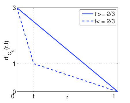
Figure 9: DMT upper bound for the cut-set around the source, $\mathcal{C}_{S}$. The source has 1, the destination has 1, and the relay has 2 antennas, $(m,n,k)=(1,1,2)$. The network is non-clustered. Note that as $m=n$, $d_{\mathcal{C}_{S}}^{\prime}(r,t)=d_{\mathcal{C}_{D}}^{\prime}(r,1-t)$. The upper bound in (43) reaches its maximum for $t=1/2$. The solid line in the figure is also equal to the full-duplex bound.

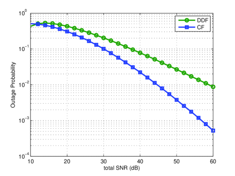
Figure 10: Outage probability versus total $\mathrm{SNR}$ for the non-clustered multiple-antenna, single half-duplex relay system, $(m,n,k)=(2,2,1)$, $r=1.5$, $t=0.5$.

In general it is hard to compute the DMT of multiple antenna DDF. This is because the instantaneous mutual information DDF achieves in a multiple antenna relay channel is equal to $I_{\mathcal{C}_{D}}(t)$ of (38) where $t$ is the random time instant at which the relay does successful decoding. Thus it is even harder to compute the DMT for this case than for fixed $t$. Moreover, we think that the multiple antenna DDF performance will still be suboptimal. In Section IV, we showed that for a multiple antenna full-duplex relay system, the probability that the relay cannot decode is dominant and the DF protocol becomes suboptimal. Therefore, we do not expect any relay decoding based protocol to achieve the DMT upper bound in the multiple antenna half-duplex system either. This conjecture is also demonstrated in Fig. 10, which shows the outage probability versus total $\mathrm{SNR}$ for DDF and CF protocols for $(m,n,k)=(2,2,1)$, $R^{(T)}=r\log(P_{S}+P_{R})$, $r=1.5$, $t=0.5$. Source has twice the power relay has. The matrices $\mathbf{H}_{SR}$, $\mathbf{H}_{SD}$ and $\mathbf{H}_{RD}$ have i.i.d. complex Gaussian entries with real and imaginary parts zero mean and variance $1/2$. We observe that the diversity gain the CF protocol achieves is approximately 0.90, whereas the DDF protocol approximately achieves 0.47.

VI The Multiple-Access Relay Channel

The most general network we introduced in Section I includes the multiple access relay channel (MARC) as a subproblem, (Problem 2). The model for MARC is shown in Fig. 11. Our emphasis is on half-duplex MARC. As in Section V without loss of generality we consider a static, fixed state protocol, where the relay listens for $t$ fraction of time, transmits for $(1-t)$ fraction and sources transmit all the time.

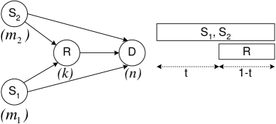
Figure 11: System model for Problem 2, the multiple access relay channel. The sources, the destination and the relay have $m_{1}$, $m_{2}$, $n$ and $k$ antennas respectively.

For the half-duplex MARC we have

$$\mathbf{Y}_{R,1} = \mathbf{H}_{S_{1}R}\mathbf{X}_{S_{1},1}+\mathbf{H}_{S_{2}R}\mathbf{X}_{S_{2},1}+\mathbf{Z}_{R,1}$$

$$\mathbf{Y}_{D,1} = \mathbf{H}_{S_{1}D}\mathbf{X}_{S_{1},1}+\mathbf{H}_{S_{2}D}\mathbf{X}_{S_{2},1}+\mathbf{Z}_{D,1}$$

at state $q_{1}$ (when the relay listens) and at state $q_{2}$ (when the relay transmits), the received signal at the destination is given as

$$\mathbf{Y}_{D,2} = \mathbf{H}_{S_{1}D}\mathbf{X}_{S_{1},2}+\mathbf{H}_{S_{2}D}\mathbf{X}_{S_{2},2}+\mathbf{H}_{RD}\mathbf{X}_{R,2}+\mathbf{Z}_{D,2}.$$

Here $\mathbf{X}_{S_{1},l}$, $\mathbf{X}_{S_{2},l}$ and $\mathbf{X}_{R,l}$ are of size $m_{1}$, $m_{2}$ and $k$ column vectors respectively and denote transmitted signal vectors at node $S_{1}$, $S_{2}$ and $R$ at state $q_{l}$, for $l=1,2$. Similarly $\mathbf{Y}_{R,l}$ and $\mathbf{Y}_{D,l}$ are the received signal vectors of size $k$ and $n$. $\mathbf{H}_{SD}$, $\mathbf{H}_{{S_{1}}D}$, $\mathbf{H}_{{S_{2}}D}$, $\mathbf{H}_{{S_{1}}R}$, $\mathbf{H}_{{S_{2}}R}$, $\mathbf{H}_{RD}$ are the channel gain matrices of size $n\times m_{1}$, $n\times m_{2}$, $k\times m_{1}$, $k\times m_{2}$, $n\times k$ respectively. The system is non-clustered.

In this section we examine the DMT for the MARC. We present our results for the MARC with single antenna nodes to demonstrate the basic idea.

The DMT upper bound for the symmetric MARC occurs when both users operate at the same multiplexing gain $r/2$, $\bar{r}=(r/2,r/2)$, and is given in [45] as

$$d_{MARC}(\bar{r})\leq\left\{\begin{array}[]{lll}2-r&\mbox{if}&0\leq r\leq\frac{1}{2}\\ 3(1-r)&\mbox{if}&\frac{1}{2}\leq r\leq 1\\ \end{array}\right.,$$ (48)

which follows from cut-set upper bounds on the information rate. Although this upper bound is a full-duplex DMT bound, it is tight enough for the half-duplex case when each node has a single antenna. We see that this upper bound has the single user DMT for $r\leq\frac{1}{2}$, and has the relay channel DMT with a two-antenna source for high multiplexing gains. This is because for low multiplexing gains, the typical outage event occurs when only one of the users is in outage, and at high multiplexing gains, the typical outage event occurs when both users are in outage, similar to multiple antenna multiple-access channels [61].

In Sections IV and V, we have observed that CF is DMT optimal for full-duplex and half-duplex multi-antenna relay channels. This motivates us to study the performance of CF in MARC.

Theorem 8

For the single antenna, half-duplex MARC the CF strategy achieves the DMT

$$d_{MARC,CF}(\bar{r})=\left\{\begin{array}[]{lll}2(1-r)&\mbox{if}&0\leq r\leq\frac{2}{3}\\ 1-\frac{r}{2}&\mbox{if}&\frac{2}{3}\leq r\leq\frac{4}{5}\\ 3(1-r)&\mbox{if}&\frac{4}{5}\leq r\leq 1\\ \end{array}\right..$$

This DMT $d_{MARC,CF}(\bar{r})$ becomes equal to the upper bound for $r\geq 4/5$.

Proof:

The proof is provided in Appendix G. ∎

To achieve the above DMT performance, two types of operation are necessary. For low multiplexing gains, $0\leq r\leq 2/3$, $S_{1}$ and $S_{2}$ utilize time sharing, and equally share the relay. Here both $S_{1}$ and $S_{2}$ transmit for the half of the total time, for $1/4$ of the whole time slot $R$ helps $S_{1}$ only, and in the last quarter, $R$ helps $S_{2}$. Then we can directly apply the results obtained in Section V, which results in the DMT $2(1-r)$ in terms of the sum multiplexing gain. For high multiplexing gains, $2/3\leq r\leq 1$, both sources transmit simultaneously. In this multiple access mode, for $4/5\leq r\leq 1$, both users being in outage is the dominant outage event, the system becomes equivalent to the multiple antenna half-duplex relay channel, and CF achieves the DMT upper bound.

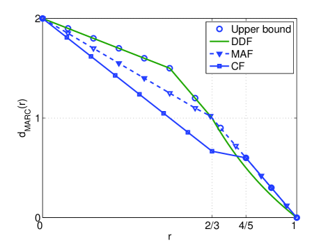
Figure 12: DMT for MARC. Each node has a single antenna.

For comparison the achievable DMT with DDF for MARC satisfies [45]:

$$d_{MARC,DDF}(r/2,r/2)\geq\left\{\begin{array}[]{lll}2-r&\mbox{if}&0\leq r\leq\frac{1}{2}\\ 3(1-r)&\mbox{if}&\frac{1}{2}\leq r\leq\frac{2}{3}\\ 2\frac{1-r}{r}&\mbox{if}&\frac{2}{3}\leq r\leq 1\\ \end{array}\right..$$

We also compare our results with the MAF protocol for the MARC channel [46, 47] in Fig. 12. The MAF performance is given as

$$d_{MARC,MAF}(r/2,r/2)=\left\{\begin{array}[]{ccc}2-3\frac{r}{2}&\mbox{if}&0\leq r\leq\frac{2}{3}\vspace{0.1 cm}\\ 3(1-r)&\mbox{if }&\frac{2}{3}\leq r\leq 1\\ \end{array}\right..$$

We observe that for low multiplexing gains, when single user outage is dominant, it is optimal to decode the sources; however for high multiplexing gains, compression works better. The MAF protocol is also optimal for high multiplexing gains.

In Section IV we observed that for a full-duplex relay channel, when terminals have multiple antennas, DF becomes suboptimal, whereas CF is not. Hence, we conjecture that DDF will not be able to sustain is optimality even in the low multiplexing gain regime when the terminals have multiple antennas. Moreover, it is not easy to extend the MAF protocol for multiple antenna MARC. Even when we have one source, the DMT for the multiple antenna NAF protocol for the relay channel is not known, only a lower bound exists [42]. On the other hand, for the multiple antenna case CF will still be optimal whenever decoding all sources together is the dominant error event. However, for some antenna numbers $m_{1}$, $m_{2}$, and $n$, single-user behavior will always dominate [61].

VII Single Antenna Nodes, Multiple Relays

In this section we examine Problem 3 and Problem 4 to see how closely a cooperative system can mimic MIMO in terms of DMT. We first study a single source destination pair with 2 relays (Problem 3) in Section VII-A, then consider two sources and destinations (Problem 4) in Section VII-B. In both cases, each node has a single antenna. We also assume the nodes are full-duplex so that we can observe the fundamental limitations a relaying system introduces.

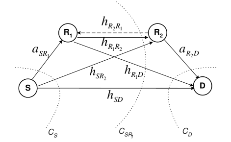
Figure 13: System model for Problem 3, the single source-destination two relay system, each node has a single antenna.

VII-A Single Source-Destination, Two Relays

In this system there is a single source-destination pair and two relays as shown in Fig. 13. The channel is characterized by

$$Y_{R_{1}} = a_{SR_{1}}X_{S}+h_{R_{2}R_{1}}X_{R_{2}}+Z_{R_{1}}$$ (50)

$$Y_{R_{2}} = h_{SR_{2}}X_{S}+h_{R_{1}R_{2}}X_{R_{1}}+Z_{R_{2}}$$ (51)

$$Y_{D} = h_{SD}X_{S}+h_{R_{1}D}X_{R_{1}}+a_{R_{2}D}X_{R_{2}}+Z_{D}$$ (52)

where $X_{i}$ and $Y_{i}$, $i=S,R_{1},R_{2},D$, are transmitted and received signals at node $i$ respectively. The channel gains $h_{ij}$, $i,j=S,R_{1},R_{2},D$, are independent, zero mean complex Gaussian with variance $2\sigma^{2}$, where $\sigma^{2}$ is defined in Section II. As discussed in Section II, we assume the $R_{2}$ to $R_{1}$ link $h_{R_{2}R_{1}}$, which is the dashed line in Fig. 13, is present only if the system is not clustered. If the system is not clustered, then the channel gains $a_{ij}$ are also Rayleigh. On the other hand, if the system is clustered, then $a_{SR_{1}}$ and $a_{R_{2}D}$ are equal to $\sqrt{G_{SR_{1}}}$ and $\sqrt{G_{R_{2}D}}$ respectively, which are the Gaussian channel gains. $Z_{i}$ denotes the AWGN noise, which is independent at each receiver. The source, the first relay, $R_{1}$, and the second relay, $R_{2}$, have power constraints $P_{S}$, $P_{R_{1}}$ and $P_{R_{2}}$ respectively. We assume the target data rate $R^{(T)}=r\log\mathrm{SNR}$. The following theorems summarize the main results of this section.

Theorem 9

The optimal DMT for the non-clustered system of Fig. 13, $d(r)$, is equal to

$$d(r)=d_{13}(r).$$

This optimal DMT is achieved when both relays employ DF strategy.

Proof:

Please refer to Appendices H and I for the DMT upper bound and achievability results respectively. ∎

Theorem 10

The optimal DMT for the clustered system of Fig. 13, where $R_{1}$ is clustered with the source and $R_{2}$ is clustered with the destination, $d(r)$ is equal to

$$d(r)=\left\{\begin{array}[]{lll}d_{22}(r)&\mbox{if}&r\leq 1\\ 0&\mbox{if}&r>1\\ \end{array}\right..$$

The mixed strategy, where $R_{1}$ does DF and $R_{2}$ does CF achieves the optimal DMT.

Proof:

Please refer to Appendices H and J for the DMT upper bound and achievability results respectively. ∎

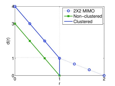
Figure 14: DMT for the single source-destination, two relay system, each node has a single antenna.

Theorem 9 says that if the system is non-clustered it can at most have a transmit or a receive antenna array DMT behavior, but cannot act as a MIMO in terms of DMT. On the other hand, Theorem 10 confirms the fact that the multiplexing gain for the clustered system is limited by 1. However, for all $r\leq 1$, the clustered system can mimic a $2\times 2$ MIMO, which means $d=1$ is achievable at $r=1$.

The DMT performances for non-clustered and clustered systems as well as $2\times 2$ MIMO are illustrated in Fig. 14. We also display the outage probability versus $\mathrm{SNR}$ for this clustered case in Fig. 15 for $R^{(T)}=r\log(P_{S}+P_{R_{1}}+P_{R_{2}})$, where $r=1$. We assumed $G_{SR_{1}}=G_{R_{2}D}=10$ and $P_{S}=P_{R_{1}}=10P_{R_{2}}$. Also, $h_{ij}$, $i,j=S,R_{1},R_{2},D$, are i.i.d. with $\sigma^{2}=1/2.$ For comparison, we also show the outage probability of a $2\times 2$ MIMO channel, where the 2 transmit antennas share the total power equally and send uncorrelated signals. The MIMO channel and the relay system have the same total power constraint. We observe that as predicted, the clustered relay network has the same diversity as the $2\times 2$ MIMO and at $r=1$, $d=1$ is achievable.

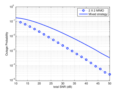
Figure 15: Outage probability for the clustered single source-destination, two relay system, each node has a single antenna. $G_{SR_{1}}=G_{R_{2}D}=10$, $r=1$.

We would like to note that for the clustered case CF is essential at $R_{2}$, and a strict decoding constraint at $R_{2}$ would limit the system performance. If both relays do DF, $R_{1}$ will always be able to decode for all multiplexing gains $0\leq r\leq 1$, as the $S-R_{1}$ channel can support rates up to $\log(1+G_{SR_{1}}P)$. Thus, it is as if there is a two-antenna transmitter. However, $R_{2}$ may or may not decode. Adapting Appendix I to the clustered case we can easily find the probability of outage at the destination from (79) as $P(\mbox{outage at D})\dot{=}\mathrm{SNR}^{-d_{31}(r)}$, which shows that the decoding constraint at $R_{2}$ limits the system performance, the system still operates as a transmit antenna array. Even though one could improve upon this strategy by using the DF protocol of [20], which allows the relays to process the signals they hear from the source and the other relay jointly, this still does not provide $2\times 2$ MIMO behavior. In this case both the destination and $R_{2}$ observe $2\times 1$ DMT, and $P(\mbox{outage at D})\dot{=}\mathrm{SNR}^{-2d_{21}(r)}=\mathrm{SNR}^{-4(1-r)}$, which is still suboptimal as it cannot achieve the upper bound of Theorem 10. Although the destination can always understand $R_{2}$ reliably (because of the clustering assumption), whenever both of them fail, the system is in outage. However, for the receive cluster, CF fits very well. If the received signal at the destination has high power due to large $h_{SD}$ and $h_{R_{1}D}$, then $R_{2}$ to destination channel has lower capacity because in the decoding process $Y_{D}$ is treated as interference. On the other hand, the correlation between the relay and destination signals is higher and a coarse description $Y_{R_{2}}$ is enough to help the destination. However, if the side information has low received power, the $R_{2}$ to destination channel has higher capacity and $R_{2}$ can send the necessary finer information as the correlation is less.

In [20, Theorem 4], the authors prove an achievable rate for a multiple relay system, in which some of the relays DF and the rest CF. Furthermore, the relays that perform CF partially decode the signals from the relays that perform DF. Performing this partial decoding leads to higher achievable rates. However, to achieve the DMT upper bound, for both the non-clustered and clustered cases, there is no need for partial decoding and a simpler strategy is enough.

Note that same multiplexing limitations in Theorem 10 would occur when the source has two antennas and a single antenna relay is clustered with a single antenna destination or the symmetric case when the destination has two antennas and a single antenna relay is clustered with a single antenna source. These multiple antenna, single source-destination, single relay cases were discussed in detail in Section IV. In addition to these, we investigate whether the multiplexing gain limitation is due to the fact that there is only a single source-destination pair in the next subsection.

VII-B Two-Source Two-Destination Cooperative System

We consider two sources and two destinations, where sources cooperate in transmission and destinations cooperate in reception (Problem 4). The system model is shown in Fig. 16. Problem 3 studied in Section VII-A would be a special case of this, if one source has no information to send.

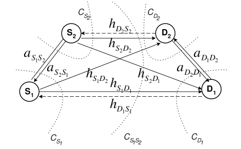
Figure 16: System model for Problem 4, the two-source two-destination system, each node has a single antenna.

First we examine the multi-cast scenario, when both destinations are required to decode both sources. This is analogous to MIMO systems and represents the information transfer from a group of antennas to another group of antennas. We define individual target data rates $R^{(T_{S_{1}})}=r_{1}\log\mathrm{SNR}$ and $R^{(T_{S_{2}})}=r_{2}\log\mathrm{SNR}$, with a sum target data rate of $R^{(T)}=r\log\mathrm{SNR}$, $r=r_{1}+r_{2}$, $\bar{r}=(r_{1},r_{2})$. Using the cut-set bounds in Fig. 16 we have the following corollary.

Corollary 2

For a multi-cast, single antenna two-source two-destination system, the system DMT $d(\bar{r})$ is upper bounded by

$$d(\bar{r})\leq d_{13}(r),$$

if the system is non-clustered, and by

$$d(\bar{r})\leq d_{22}(r),~{}0\leq r\leq 1,$$

if the system is clustered. Here $r=r_{1}+r_{2}$ is the sum multiplexing gain of the system, and this upper bound is maximized for $\bar{r}=(r/2,r/2)$.

We omit the proof, which is very similar to the upper bound calculation in Section VII-A.

We observe that cooperative multicast is still limited in multiplexing gains. We next study study the cooperative interference channel, where $D_{1}$ is only required to decode $S_{1}$ and $D_{2}$ to decode $S_{2}$. The cooperative interference channel imposes looser decoding requirements on the destinations and potentially leads to higher achievable rates. The next corollary shows that for the clustered cooperative interference channel it is still not possible to achieve multiplexing gains above $r=1$. Hence, we conclude the multiplexing gain limitation is not due to having one source-destination, but is due to the finite capacity links within each cluster.

Corollary 3

A single antenna two-source two-destination, clustered cooperative interference channel has the best DMT as

$$\max_{r_{1}+r_{2}=r}d(\bar{r})=d_{22}(r),~{}0\leq r\leq 1.$$

Proof:

We can show that $d(\bar{r})\leq d_{22}(r)$ using the upper bound of Lemma 1. The result in [50] suggests that for cooperative interference channel the total multiplexing gain can be at most 1. Thus we have $d(\bar{r})\leq d_{22}(r),~{}0\leq r\leq 1.$

A simple achievable scheme assumes that ($S_{1}$, $D_{1}$) pair uses ($S_{2}$, $D_{2}$) pair as relays for half of the transmission period to send $R^{(T_{S_{1}})}=r/2\log\mathrm{SNR}$. In the remaining half $S_{2}$ sends $R^{(T_{S_{2}})}=r/2\log\mathrm{SNR}$ to $D_{2}$ utilizing $S_{1}$ and $D_{1}$ as relays. Note that equal distribution of rates gives the best network diversity, since any other distribution of $r_{1}$ and $r_{2}$ leads to a lower diversity for one of the streams. Then, for each case, the problem reduces to the one discussed in Section VII-A. We can easily show that this strategy meets the DMT upper bound and that using such a time division scheme is DMT optimal for the cooperative interference channel. ∎

For comparison, suppose there were two clustered single antenna sources and a single two-antenna destination. This system can be a virtual MIMO, achieving the full $2\times 2$ MIMO DMT, unlike the single-antenna two-source two-destination system described above. In this case, when high diversity gains are needed, the sources can cooperate, decode and forward each other’s signals using time division, and collectively act as a two-antenna transmitter similar to the above argument. For high multiplexing gains, they simply operate in the multiple access mode, i.e. each source sends its own independent information stream, and thus can attain all multiplexing gains up to 2 [37]. However, if we had a two-antenna source and two clustered single antenna destinations, the system would be multiplexing gain limited, as CSI is not available at the transmitter [62]. All these examples emphasize the difference between transmit and receive clusters, in addition to the effect of finite capacity links within each cluster.

VIII Conclusion

In this work we find the diversity-multiplexing tradeoff (DMT) for the following subproblems of a general multiple antenna network with multiple sources, multiple destinations and multiple relays: 1) A single source-destination system, with one relay, each node has multiple antennas, 2) The multiple-access relay channel with multiple sources, one destination and one relay, each node has multiple antennas, 3) A single source-destination system with two relays, each node has a single antenna, 4) A multiple source-multiple destination system, each node has a single antenna. For different configurations we consider the effect of half-duplex or full-duplex behavior of the relay as well as clustering.

Firstly, we study a full-duplex multi-antenna relay system DMT. We examine the effect of clustering on both the DMT upper bounds and achievability results. We compare a single-antenna relay system with a multiple-antenna relay system, when the source, the destination and the relay have $m$, $n$ and $k$ antennas respectively, and investigate the effects of increased degrees of freedom on the relaying strategies decode-and-forward, and compress-and-forward. We find that multi-antenna relay systems have fundamental differences from their single-antenna counterparts. Increased degrees of freedom affects the DMT upper bounds and the performance of different relaying strategies leading to some counterintuitive results. Although the DF protocol is simple and effective to achieve the DMT upper bounds in single antenna relay systems, it can be suboptimal for multi-antenna relay systems, even if the relay has the same number of antennas as the source. On the other hand, the CF strategy is highly robust and achieves the DMT upper bounds for all multiplexing gain values for both clustered and non-clustered networks. Clustering is essential for DF to achieve the DMT upper bound for low multiplexing gains, but does not help in the high multiplexing gain region. What’s more, it has an adverse effect on both the upper bound and the DF achievable DMT if the relay has multiple antennas due to decreased degrees of freedom in the source-relay channel.

We extend the above full-duplex results obtained for the multiple antenna relay channel to the half-duplex relay as well. We show that for the multiple-antenna half-duplex relay channel the CF protocol achieves the DMT upper bound. Although it is hard to find the DMT upper bound explicitly for arbitrary $m$, $n$ and $k$, we have solutions for special cases. We show that the half-duplex DMT bound is tighter than the full-duplex bound in general, and CF is DMT optimal for any $m$, $n$ and $k$. We also argue that the dynamic decode-and-forward protocol or any decoding based protocol would be suboptimal in the multiple antenna half-duplex relay channel as they are suboptimal in the full-duplex case.

We next investigate the multiple-access relay channel. In MARC, CF achieves the upper bound for high multiplexing gains, when both users being in outage is the dominant outage event.

Finally, we compare wireless relay and cooperative networks with a physical multi-input multi-output system. We show that despite the common belief that the relay or cooperative systems can be virtual MIMO systems, this is not possible for all multiplexing gains. Both for relay and cooperative systems, even if the nodes are clustered, the finite capacity link between nodes in the source cluster and the finite capacity link between the nodes in the destination cluster are bottlenecks and limit the multiplexing gain of the system. Cooperative interference channels are also limited the same way. It is straightforward to extend our results for a single source-destination pair with multiple relays and for cooperative systems with N sources and N destinations with each destination decoding all sources.

Overall, our results indicate the importance of soft information transmission in relay networks, as in CF, and suggest that protocol design taking into account node locations, antenna configurations and transmission/reception constraints are essential to harvest diversity and multiplexing gains in cooperative systems.

Appendix A Proof of Lemma 1

By Proposition 1, the information rates $R^{(kl)}$ from node $k$ to node $l$ in the network satisfy

$$\sum_{k\in\mathcal{C}_{i},l\in\mathcal{C}_{i}^{c}}R^{(kl)} \leq I_{\mathcal{C}_{i}}$$

for some $p(x_{1},x_{2},...,x_{m})$. Also, we can easily observe that $\mathcal{E}_{N}$ is implied by the event

$$\sum_{k\in\mathcal{C}_{i},l\in\mathcal{C}_{i}^{c}}R^{(kl)}<R^{(T_{\mathcal{C}_{i}})}.$$

Then for any coding scheme with rates $R^{(kl)}$, we can write

$$P\left(\mathcal{E}_{N}\right) \geq P\left(\sum_{k\in\mathcal{C}_{i},l\in\mathcal{C}_{i}^{c}}R^{(kl)}<R^{(T_{\mathcal{C}_{i}})}\right)$$

$$\geq P(I_{\mathcal{C}_{i}}<R^{(T_{\mathcal{C}_{i}})})$$

$$\geq \min_{p(x_{1},x_{2},...,x_{m})}P(I_{\mathcal{C}_{i}}<R^{(T_{\mathcal{C}_{i}})}).$$

The above statement holds for all coding schemes with rates $R^{(kl)}$; thus, it is also true for the one that minimizes the left hand side. Then we have

$$\min_{\mbox{\tiny{all coding schemes}}}P\left(\mathcal{E}_{N}\right)\geq\min_{p(x_{1},x_{2},...,x_{m})}P(I_{\mathcal{C}_{i}}<R^{(T_{\mathcal{C}_{i}})})$$ (54)

The right hand side is the minimum outage probability for cut-set $\mathcal{C}_{i}$, and by the definition in the lemma

$$\min_{p(x_{1},x_{2},...,x_{m})}P(I_{\mathcal{C}_{i}}<R^{(T_{\mathcal{C}_{i}})})\dot{=}\mathrm{SNR}^{-d_{\mathcal{C}_{i}}(r^{(\mathcal{C}_{i})})}.$$ (55)

Using the definition of maximum network diversity, we have

$$\min_{\mbox{\tiny{all coding schemes}}}P\left(\mathcal{E}_{N}\right)\dot{=}\mathrm{SNR}^{-d(\bar{r})}.$$ (56)

Substituting (55) and (56) into (54) leads to

$$d(\bar{r})\leq d_{\mathcal{C}_{i}}(r^{(\mathcal{C}_{i})}).$$

Since this is true for all the cut-sets, we have

$$d(\bar{r})\leq\min_{i}d_{\mathcal{C}_{i}}(r^{(\mathcal{C}_{i})}).$$

We conclude that the maximum network diversity order $d(\bar{r})$ is upper bounded by the maximum diversity order of each $I_{\mathcal{C}_{i}}$.

Appendix B Proof of Theorem 2

In the DF protocol, the source and the relay employ block Markov superposition coding [55, 20] and the destination does backward decoding [20, 58, 59]. For achievability, we constrain the relay to decode the source signal reliably. If based on its received $\mathrm{SNR}$ the relay cannot decode, then it remains silent (or sends a default signal). We assume this is known at the destination, which can be communicated at a negligible cost. Since fading is constant for all $B$ blocks, this has to be communicated only once.

The relay decodes if the instantaneous mutual information satisfies

$$R^{(DF)}\leq I(\mathbf{X}_{S};\mathbf{Y}_{R}|\mathbf{X}_{R}).$$

If the relay can decode, the mutual information at the destination is $I(\mathbf{X}_{S}\mathbf{X}_{R};\mathbf{Y}_{D})$, otherwise it is $I(\mathbf{X}_{S};\mathbf{Y}_{D}|\mathbf{X}_{R})$. We choose $\mathbf{X}_{S}$ and $\mathbf{X}_{R}$ independently as complex Gaussian with zero mean with covariance matrices $Q_{S}=\mathbf{I}_{m}P_{S}/m$, and $Q_{R}=\mathbf{I}_{k}P_{R}/k$ respectively. Then we can write

$$I(\mathbf{X}_{S};\mathbf{Y}_{R}|\mathbf{X}_{R}) = \log L_{S,R}$$

$$I(\mathbf{X}_{S};\mathbf{Y}_{D}|\mathbf{X}_{R}) = \log L_{S,D}$$

$$I(\mathbf{X}_{S}\mathbf{X}_{R};\mathbf{Y}_{D}) = \log L_{SR,D},$$

where

$$L_{S,R}=\left|\mathbf{I}_{k}+\mathbf{H}_{SR}\mathbf{H}_{SR}^{\dagger}\frac{P_{S}}{m}\right|,$$

and $L_{S,D}$ and $L_{SR,D}$ are defined in (16) and (17) respectively.

We calculate the probability of outage as

$$P(\mbox{outage at D})$$

$$= P(\mbox{outage}|\mbox{relay decodes})P(\mbox{relay decodes})$$

$${+}\>P(\mbox{outage}|\mbox{relay cannot decode})$$

$${.}\>P(\mbox{relay cannot decode})$$

$$= P(L_{SR,D}<\mathrm{SNR}^{r})P(L_{S,R}>\mathrm{SNR}^{r})$$

$${+}\>P(L_{S,D}<\mathrm{SNR}^{r})P(L_{S,R}<\mathrm{SNR}^{r})$$

$$\dot{=} \left\{\begin{array}[]{l}{\mathrm{SNR}^{-d_{(m+k)n}(r)}}+{\mathrm{SNR}^{-d_{mn}(r)}}{\mathrm{SNR}^{-d_{mk}(r)}}\\ ~{}~{}~{}~{}~{}~{}~{}~{}~{}~{}~{}~{}~{}~{}~{}~{}~{}~{}~{}~{}~{}~{}~{}~{}~{}\mbox{if~{}}0\leq r\leq\min\{m,n,k\}\\ {\mathrm{SNR}^{-d_{mn}(r)}}\\ ~{}~{}~{}~{}~{}~{}~{}~{}~{}~{}~{}~{}~{}\mbox{if~{}}\min\{m,n,k\}<r\leq\min\{m,n\}\end{array}\right.$$ (62)

for which we used the fact that $P(L_{S,R}>\mathrm{SNR}^{r})\dot{=}1$ for $0\leq r\leq\min\{m,n,k\}$, and for $\min\{m,n,k\}<r\leq\min\{m,n\}$, $P(L_{S,R}>\mathrm{SNR}^{r})\dot{=}0$ and $P(L_{S,R}<\mathrm{SNR}^{r})\dot{=}1$. Hence we can write the DMT for DF as in (33). Note that any other choice of $Q_{S}$, $Q_{R}$ and $Q=\mathrm{Cov}(\mathbf{X}_{S},\mathbf{X}_{R})$ would not improve this result. This is because for any $Q_{S}$, $Q_{R}$ and $Q$, due to (1), the mutual information expressions have the upper bounds

$$I(\mathbf{X}_{S};\mathbf{Y}_{R}|\mathbf{X}_{R}) \leq \log\left|\mathbf{I}_{k}+\mathbf{H}_{SR}\mathbf{H}_{SR}^{\dagger}P_{S}\right|$$

$$I(\mathbf{X}_{S};\mathbf{Y}_{D}|\mathbf{X}_{R}) \leq \log\left|\mathbf{I}_{n}+\mathbf{H}_{SD}\mathbf{H}_{SD}^{\dagger}P_{S}\right|$$

and

$$I(\mathbf{X}_{S}\mathbf{X}_{R};\mathbf{Y}_{D}) \leq \log K_{SR,D}$$

where $K_{SR,D}$ is defined in (9). A DMT calculation using these upper bounds would result in the same DMT as in (33).

Appendix C Proof of Theorem 4

First, the mutual information for cut-set $\mathcal{C}_{D}$ is the same as the non-clustered case of (5), and the DMT upper bound for this cut-set is $d_{(m+k)n}(r)$. For cut-set $\mathcal{C}_{S}$ we need to find the DMT for the channel

$$\mathbf{Y}={\mathbf{H}_{S,RD}}\mathbf{X}+\mathbf{Z},$$

where $\mathbf{H}_{S,RD}$ is defined in (13), $\mathbf{H}_{SR}$ is an $k\times m$ matrix with all entries equal to $\sqrt{G}$, and $\mathbf{H}_{SD}$ is $n\times m$, with complex Gaussian entries $h_{ij}$, $i=1,...,n$, $j=1,2$. The channel input $\mathbf{X}$ is $m\times 1$ and has the total transmit power constraint $P_{S}$. We assume $P_{S}=\mathrm{SNR}$ for notational simplicity in this appendix. The channel output, $\mathbf{Y}$, and the complex Gaussian noise at the output, $\mathbf{Z}$, are $(n+k)\times 1$.

For $m=1$, the DMT is easily calculated as $d_{\mathcal{C}_{S}}(r)=\infty$, $0\leq r\leq 1$, as $I_{\mathcal{C}_{S}}>\log(1+kGP_{S})$.

For $m=2$, the instantaneous mutual information for a given channel gain matrix $\mathbf{H}_{S,RD}$ is then

$$I\left(\mathbf{X};\mathbf{Y}\right) = \log\left|\mathbf{I}_{2}+\mathrm{SNR}\mathbf{H}_{S,RD}^{{\dagger}}\mathbf{H}_{S,RD}\right|.$$

Note that

$$\mathbf{H}_{S,RD}^{{\dagger}}\mathbf{H}_{S,RD} = \left[\mathbf{H}_{SR}^{\dagger}\mathbf{H}_{SR}+\mathbf{H}_{SD}^{\dagger}\mathbf{H}_{SD}\right]$$

$$= \left[\left(\begin{array}[]{cc}kG&kG\\ kG&kG\\ \end{array}\right)+\mathbf{H}_{SD}^{\dagger}\mathbf{H}_{SD}\right],$$

which means having $k$ relay antennas only increases the Gaussian channel gain in between the source and the relay antennas by a constant factor. Therefore, without loss of generality we can assume $k=1$. For $k=1$,

$${I(\mathbf{X};\mathbf{Y})} = \log\left(1+2G\mathrm{SNR}+\Sigma_{i=1}^{n}\Sigma_{j=1}^{2}|h_{ij}|^{2}\mathrm{SNR}+\right.$$

$${+}\>\left.\Sigma_{i=1}^{n}|h_{i1}-h_{i2}|^{2}G\mathrm{SNR}\right.$$

$${+}\>\left.\Sigma_{i=1}^{n}\Sigma_{j=i+1}^{n}|h_{i1}h_{j2}-h_{i2}h_{j1}|^{2}\mathrm{SNR}^{2}\right).$$

There is no outage for multiplexing gain $r\leq 1$ as $I(\mathbf{X};\mathbf{Y})\geq\log(1+2G\mathrm{SNR})$. For $1<r\leq 2$, we can lower bound the outage probability as

$$P(\mbox{outage}) = P(\mbox{outage}|\mathcal{E})P(\mathcal{E})+P(\mbox{outage}|\mathcal{E}^{c})P(\mathcal{E}^{c})$$

$$\geq P(\mbox{outage}|\mathcal{E})P(\mathcal{E}),$$

where

$${\mathcal{E}} = \left\{|\Re\{h_{i1}\}-\Re\{h_{i2}\}|<\epsilon,|\Im\{h_{i1}\}-\Im\{h_{i2}\}|<\epsilon:\right.$$

$$\left.i=1,...,n\right\}$$

with $\epsilon=1/\sqrt{\mathrm{SNR}^{2-r}}$. When $\mathcal{E}$ holds,

$$I(\mathbf{X};\mathbf{Y}) = \log\left(1+2G\mathrm{SNR}+\Sigma_{i=1}^{n}\Sigma_{j=1}^{2}|h_{ij}|^{2}\mathrm{SNR}\right.$$

$${+}\>\left.2\epsilon^{2}nG\mathrm{SNR}\right.$$

$${+}\>\left.2\epsilon^{2}\Sigma_{i=1}^{n}\Sigma_{j=i+1}^{n}|h_{i1}-h_{j1}|^{2}\mathrm{SNR}^{2}\right).$$

Then for a target data rate $R^{(T)}=r\log\mathrm{SNR}$, we have

$${P(\mbox{outage}|\mathcal{E})} = P\left(\Sigma_{i=1}^{n}\Sigma_{j=1}^{2}|h_{ij}|^{2}\frac{1}{\mathrm{SNR}^{r-1}}\right.$$

$${+}\>\left.2\Sigma_{i=1}^{n}\Sigma_{j=i+1}^{n}|h_{i1}-h_{j1}|^{2}<f(\mathrm{SNR})\right),$$

where

$$f(\mathrm{SNR})=\frac{\mathrm{SNR}^{r}-1-2G\mathrm{SNR}-2nG\mathrm{SNR}^{r-1}}{\mathrm{SNR}^{r}}.$$

Then for $\mathrm{SNR}>1$, $1/\mathrm{SNR}^{r-1}<1$, therefore, we can further lower bound $P(\mbox{outage}|\mathcal{E})$ as

$$P(\mbox{outage}|\mathcal{E}) \geq P\left(\Sigma_{i=1}^{n}\Sigma_{j=1}^{2}|h_{ij}|^{2}\right.$$

$${+}\>\left.2\Sigma_{i=1}^{n}\Sigma_{j=i+1}^{n}|h_{i1}-h_{j1}|^{2}<f(\mathrm{SNR})\right).$$

As $f(\mathrm{SNR})\dot{=}1$, then $P(\mbox{outage}|\mathcal{E})\dot{=}1$. On the other hand, as the real and imaginary parts of all random variables are i.i.d. we have

$$P(\mathcal{E})=(P(|\Re\{h_{i1}\}-\Re\{h_{i2}\}|<\epsilon))^{2n},$$

and

$$P(|\Re\{h_{i1}\}-\Re\{h_{i2}\}|<\epsilon)$$

$$= \int_{-\infty}^{\infty}\int_{x-\epsilon}^{x+\epsilon}\frac{1}{\pi}e^{-y^{2}-x^{2}}dydx$$

$$= \int_{-\infty}^{\infty}\int_{-\epsilon}^{\epsilon}\frac{1}{\pi}e^{-(t+x)^{2}}e^{-x^{2}}dtdx$$

$$= \int_{-\epsilon}^{\epsilon}\int_{-\infty}^{\infty}\frac{1}{\pi}e^{-2x^{2}-2tx}e^{-t^{2}}dxdt$$

$$= \int_{-\epsilon}^{\epsilon}\frac{1}{\sqrt{2\pi}}e^{-t^{2}/2}dt$$

$$= \mathrm{erf}\left(\frac{\epsilon}{\sqrt{2}}\right).$$

The error function has the Maclaurin series expansion of

$$\mathrm{erf}(x)=\frac{2}{\sqrt{\pi}}\left(x-\frac{1}{3}x^{3}+\frac{1}{10}x^{5}-\frac{1}{42}x^{7}+...\right),$$

which makes $\mathrm{erf}(\epsilon/\sqrt{2})\dot{=}\epsilon$ at high $\mathrm{SNR}$. Then $P(\mathcal{E})\dot{=}\epsilon^{2n}=\mathrm{SNR}^{-2n+nr},$ and we have

$$P(\mathrm{outage})\dot{\geq}\mathrm{SNR}^{-2n+nr}.$$

On the other hand,

$$P(\mathrm{outage})$$

$$\leq P\left(\log\left|\mathbf{I}_{2}+\mathrm{SNR}\tilde{\mathbf{H}}_{S,RD}^{\dagger}\tilde{\mathbf{H}}_{S,RD}^{\dagger}\right|<r\log\mathrm{SNR}\right)$$

$$\dot{=} \mathrm{SNR}^{-2n+nr},$$

where $\tilde{\mathbf{H}}_{S,RD}^{\dagger}=\left[\tilde{\mathbf{H}}_{SR}^{\dagger}~{}\mathbf{H}_{SD}^{\dagger}\right]$, and $\tilde{\mathbf{H}}_{SR}$ is an $1\times m$ matrix with i.i.d. complex Gaussian entries.

Thus, for $1<r\leq 2$, $d_{\mathcal{C}_{S}}(r)$ is equal to the DMT of a $2\times(n+1)$ system, $d_{2(n+1)}(r)=n(2-r)$, and overall we have the $d(r)$ expression stated in Theorem 4 for $m=1,2$ and arbitrary $n$ and $k$.

Appendix D Proof of Lemma 4

In random state half-duplex relay systems, the system state can also be viewed as a channel input. Thus, we need to optimize over all joint distributions $p(x_{S},x_{R},q)$. Using Proposition 1 we have

$$R^{(SD)}\leq\min_{i}I_{\mathcal{C}_{i}},$$

$i=S,D$, for some $p(x_{S},x_{R},q)$, where $R^{(SD)}$ is the information rate from $S$ to $D$. Then for a target data rate $R^{(T)}=r\log\mathrm{SNR}$ we have

$$\min_{\mbox{all coding schemes}}P\left(R^{(SD)}<R^{(T)}\right)$$

$$\geq \min_{p(x_{S},x_{R},q)}\max_{i}P(I_{\mathcal{C}_{i}}<R^{(T)})$$

$$\geq \min_{p(q)}\max_{i}\min_{p(p(x_{S},x_{R}|q))}P(I_{\mathcal{C}_{i}}<R^{(T)}).$$

Then using (36) we can write

$$d({r})\leq\max_{p(q)}\min_{i}d_{\mathcal{C}_{i}}(r,p(q)).$$

For the multiple antenna, half-duplex relay channel we have

$$I_{\mathcal{C}_{S}} = I(X_{S},Q;Y_{R},Y_{D}|X_{R})$$

$$= I(X_{S};Y_{R},Y_{D}|X_{R},Q)+I(Q;Y_{R},Y_{D}|X_{R})$$

$$\leq I(X_{S};Y_{R},Y_{D}|X_{R},Q)+1$$

where the last inequality follows because $Q$ is a binary random variable. Similarly,

$$I_{\mathcal{C}_{D}} = I(X_{S},X_{R},Q;Y_{D})$$

$$= I(X_{S},X_{R};Y_{D}|Q)+I(Q;Y_{D})$$

$$\leq I(X_{S},X_{R};Y_{D}|Q)+1.$$

The above two bounds show that random state protocols can at most send one extra bit of information, which does not play a role at high $\mathrm{SNR}$. Thus, fixed and random state protocols have the same DMT upper bound.

Appendix E Proof of Theorem 6

To illustrate that CF achieves the DMT in Theorem 6, we follow the CF protocol of Section IV. In the static half-duplex case the relay listens to the source only for $t$ fraction of time with $0\leq t\leq 1$. The Wyner-Ziv type compression rate is such that the compressed signal at the relay can reach the destination error-free in the remaining $(1-t)$ fraction of time, in which the relay transmits. Then, for a fixed $t$ the instantaneous mutual information at the destination is

$$R^{(CF)}=tI(\mathbf{X}_{S};\hat{\mathbf{Y}}_{R}\mathbf{Y}_{D}|q_{1})+(1-t)I(\mathbf{X}_{S};\mathbf{Y}_{D}|\mathbf{X}_{R},q_{2})$$

subject to

$$tI(\hat{\mathbf{Y}}_{R};\mathbf{Y}_{R}|\mathbf{Y}_{D},q_{1})\leq(1-t)I(\mathbf{X}_{R};\mathbf{Y}_{D}|q_{2}).$$ (64)

Note that the above equations incorporate the half-duplex constraint into (14) and (15). The source and relay input distributions are independent, $\hat{\mathbf{Y}}_{R}$ is the auxiliary random vector which denotes the compressed signal at the relay and depends on $\mathbf{Y}_{R}$ and $\mathbf{X}_{R}$. More information on CF can also be found in [14, 21, 22] for the half-duplex case for single antenna nodes.

We consider $\mathbf{X}_{S}$ and $\mathbf{X}_{R}$ are i.i.d. complex Gaussian with zero mean and covariance matrices $\mathbf{I}_{m}P_{S}/m$, $\mathbf{I}_{k}P_{R}/k$, $\hat{\mathbf{Y}}_{R}=\mathbf{Y}_{R,1}+\hat{\mathbf{Z}}_{R}$, and $\hat{\mathbf{Z}}_{R}$ is a vector with i.i.d. complex Gaussian entries with zero mean and variance $\hat{N}_{R}$ that is independent from all other random variables. Using the definitions of $L_{S,D}$, $L_{SR,D}$, $L_{S,RD}$, and $L_{S,RD}^{\prime}$ (16), (17), (20) and (21) we have

$$I(\hat{\mathbf{Y}}_{R};\mathbf{Y}_{R}|\mathbf{Y}_{D},q_{1}) = \log\frac{L_{S,RD}}{L_{S,D}\hat{N}_{R}^{k}},$$

$$I(\mathbf{X}_{R};\mathbf{Y}_{D}|q_{2}) = \log\frac{L_{SR,D}}{L_{S,D}}.$$

Thus using (64) we can choose the compression noise variance $\hat{N}_{R}$ to satisfy

$$\hat{N}_{R}=\sqrt[k]{\frac{L_{S,RD}}{U}},\mbox{~{}with~{}}U=L_{S,D}\left(\frac{L_{SR,D}}{L_{S,D}}\right)^{(\frac{1-t}{t})},$$

and (E) becomes

$$R^{(CF)}=t\log\frac{L_{S,RD}}{\left({\hat{N}_{R}}+1\right)^{k}}+(1-t)\log L_{S,D}.$$ (65)

To prove the DMT of (65) we follow steps similar to (23)-(27). Then we have

$$P(\mbox{outage at D})$$

$$= P\left(R^{(CF)}<r\log\mathrm{SNR}\right)$$

$$= P\left({L_{S,RD}^{\prime}}^{t}L_{S,D}^{(1-t)}<2^{kt}\mathrm{SNR}^{r}\right)$$

$${+}\>P\left(L_{SR,D}^{(1-t)}L_{S,D}^{t}<2^{kt}\mathrm{SNR}^{r}\right)$$

$$\overset{(a)}{\leq} P\left({L_{S,RD}^{\prime}}^{t}L_{S,D}^{(1-t)}<2^{k}\mathrm{SNR}^{r}\right)$$

$${+}\>P\left(L_{SR,D}^{(1-t)}L_{S,D}^{t}<2^{k}\mathrm{SNR}^{r}\right)$$

$$= P\left(t\log{L_{S,RD}^{\prime}}\right.$$

$${+}\>\left.(1-t)\log L_{S,D}<r\log\sqrt[r]{2^{k}}\mathrm{SNR}\right)$$

$${+}\>P\left((1-t)\log L_{SR,D}\right.$$

$${+}\>\left.t\log L_{S,D}<r\log\sqrt[r]{2^{k}}\mathrm{SNR}\right)$$

$$\overset{(b)}{\dot{=}} \mathrm{SNR}^{-d_{\mathcal{C}_{S}}^{\prime}(r,t)}+\mathrm{SNR}^{-d_{\mathcal{C}_{D}}^{\prime}(r,t)}$$

$$\dot{=} \mathrm{SNR}^{-\min\{d_{\mathcal{C}_{S}}^{\prime}(r,t),d_{\mathcal{C}_{D}}^{\prime}(r,t)\}},$$

where $(a)$ is because for any fixed $0\leq t\leq 1$, $2^{k}>2^{kt}$. For $(b)$ we have used the fact that $L_{S,RD}^{\prime}$ and $K_{S,RD}^{\prime}$, $L_{S,D}$ and $K_{S,D}$, and $L_{SR,D}$ and $K_{SR,D}$ are of the same form except for power scaling and hence result in the same DMT. As a result if $P(\mbox{outage at D})\dot{=}\mathrm{SNR}^{-d(r,t)}$, then $d(r,t)\geq\min\{d_{\mathcal{C}_{S}}^{\prime}(r,t),d_{\mathcal{C}_{D}}^{\prime}(r,t)\}$. As the achievable DMT cannot be larger than the upper bound, we conclude that CF achieves the bound in (42) for any $t$. Thus it also achieves the best upper bound of (43).

If the relay is dynamic, CF can also behave dynamically and $t$ will be a function of CSI available at the relay. For dynamic CF we can still upper bound the probability of outage at the destination with (E), which is equivalent to the DMT upper bound for dynamic protocols at high $\mathrm{SNR}$. Hence, dynamic CF achieves the dynamic half-duplex DMT upper bound.

Appendix F Proof of Theorem 7

In this appendix we prove Theorem 7. For $m=1$, (40) can be written as

$$I_{\mathcal{C}_{S}}^{\prime}(t)=t\log K_{S,RD}^{\prime}+(1-t)\log K_{S,D},$$

with

$$K_{S,RD}^{\prime} = \log\left(1+\sum_{i=1}^{n+k}x_{i}\mathrm{SNR}\right)$$

$$K_{S,D} = \log\left(1+\sum_{i=1}^{n}x_{i}\mathrm{SNR}\right)$$

where $x_{i}$ are independent exponentially distributed random variables with parameter 1, that denote the fading power from source antenna to receive antenna $i$ at the destination or at the relay respectively.

Let $x_{i}=\mathrm{SNR}^{-\alpha_{i}}$, $i=1,...,n+k$. Then $\alpha_{i}$ are i.i.d. with probability density function

$$f_{\alpha_{i}}(\alpha_{i})=\log(\mathrm{SNR})\mathrm{SNR}^{-\alpha_{i}}\mathrm{exp}(-\mathrm{SNR}^{-\alpha_{i}}).$$

Let $\mathcal{A}$ denote the outage event for a target data rate $R^{(T)}=r\log\mathrm{SNR}$. Then probability of outage is

$$P(\mathcal{A})$$

$$= P(I_{\mathcal{C}_{S}}^{\prime}(t)<r\log\mathrm{SNR})$$

$$= \int_{\mathcal{A}}f_{\bm{\alpha}}(\bm{\alpha})d\bm{\alpha}$$

$$= \int_{\mathcal{A}}(\log\mathrm{SNR})^{n+k}\mathrm{SNR}^{-\Sigma\alpha_{i}}\exp(-\Sigma\mathrm{SNR}^{-\alpha_{i}})d\bm{\alpha}$$

$$\overset{(a)}{\dot{=}} \int_{\mathcal{A}\bigcap\mathbb{R}^{(n+k)+}}\mathrm{SNR}^{-\Sigma\alpha_{i}}d\bm{\alpha}$$

$$\overset{(b)}{\dot{=}} \int_{\mathcal{\tilde{A}}\bigcap\mathbb{R}^{(n+k)+}}\mathrm{SNR}^{-\Sigma\alpha_{i}}d\bm{\alpha}$$

$$\overset{(c)}{\dot{=}} \mathrm{SNR}^{-G^{*}}$$

where $\mathbb{R}^{(n+k)+}$ is the set of real $(n+k)$-vectors with nonnegative elements. The outage event $\mathcal{\tilde{A}}$ is defined as

$$\mathcal{\tilde{A}} = \left\{t\max\{0,1-\alpha_{1},1-\alpha_{n+1}\right.\}$$

$${+}\>\left.(1-t)\max\{0,1-\alpha_{1}\}<r\right\}$$

where without loss of generality we assume $\alpha_{1}=\min\{\alpha_{1},...\alpha_{n}\}$ and $\alpha_{n+1}=\min\{\alpha_{n+1},...,\alpha_{n+k}\},$ and $G^{*}$ is given as

$$G^{*}=\inf_{\alpha\in\mathcal{\tilde{A}}\bigcap\mathbb{R}^{(n+k)+}}\Sigma_{i=1}^{n+k}\alpha_{i}.$$ (68)

We have $(a)$ because $(\log\mathrm{SNR})^{n+k}$ does not change the diversity gain, $\exp\left(-\mathrm{SNR}^{-\alpha_{i}}\right)$ decays exponentially with $\mathrm{SNR}$ if $\alpha_{i}<0$, $\exp\left(-\mathrm{SNR}^{-\alpha_{i}}\right)$ is $e$ for $\alpha_{i}=0$ and $\exp\left(-\mathrm{SNR}^{-\alpha_{i}}\right)$ approaches 1 for $\alpha_{i}>0$ at high $\mathrm{SNR}$ [37], $(b)$ follows because at high $\mathrm{SNR}$ $\mathcal{A}$ converges to $\mathcal{\tilde{A}}$, finally $(c)$ is due to Laplace’s method [37].

As a result $d_{\mathcal{C}_{S}^{\prime}}(r,t)=G^{*}$. To solve the optimization problem of (68). we first solve the subproblems

$$s_{i}\triangleq\inf_{\alpha\in\mathcal{\tilde{A}}\bigcap\mathbb{R}^{(n+k)+}\bigcap\mathcal{S}_{i}}\Sigma_{i=1}^{n+k}\alpha_{i},$$

where

$$\mathcal{S}_{1} = \{(\alpha_{1},\alpha_{n+1})|0\leq\alpha_{n+1}\leq 1\leq\alpha_{1}\}$$

$$\mathcal{S}_{2} = \{(\alpha_{1},\alpha_{n+1})|0\leq\alpha_{1}\leq\alpha_{n+1}\leq 1\}$$

$$\mathcal{S}_{3} = \{(\alpha_{1},\alpha_{n+1})|0\leq\alpha_{n+1}\leq\alpha_{1}\leq 1\}$$

$$\mathcal{S}_{4} = \{(\alpha_{1},\alpha_{n+1})|0\leq\alpha_{1}\leq 1\leq\alpha_{n+1}\}$$

$$\mathcal{S}_{5} = \{(\alpha_{1},\alpha_{n+1})|1\leq\alpha_{1},\alpha_{n+1}\}.$$

As an example, suppose we want to find $s_{1}$. Thus we have the following linear optimization problem

$$\mbox{minimize~{}}\Sigma_{i=1}^{n+k}\alpha_{i}$$

$$t(1-\alpha_{n+1})-r \leq 0$$

$$0~{}\leq~{}\alpha_{n+1}~{}\leq~{}1 \leq \alpha_{1}$$

$$\min\{\alpha_{1},...\alpha_{n}\} = \alpha_{1}$$

$$\min\{\alpha_{n+1},...,\alpha_{n+k}\} = \alpha_{n+1}$$

This problem has two solutions at

$$(\alpha_{1}^{*},...,\alpha_{n}^{*},\alpha_{n+1}^{*},...,\alpha_{n+k}^{*})$$

$$= \left\{\begin{array}[]{lll}(1,...,1,0,...0)&\mbox{if}&t\leq r\\ (1,...,1,1-r/t,...,1-r/t)&\mbox{if}&t\geq r\\ \end{array}\right..$$

Then for $\alpha\in\mathcal{\tilde{A}}\bigcap\mathbb{R}^{(n+k)+}\bigcap\mathcal{S}_{1}$

$$s_{1}=\min\Sigma\alpha_{i}=\left\{\begin{array}[]{lll}n&\mbox{if}&t\leq r\\ n+k(1-r/t)&\mbox{if}&t\geq r\\ \end{array}\right..$$

Similarly, we find $s_{2},s_{3},s_{4}$ and $s_{5}$. Then $G^{*}=\min_{i}s_{i}$, which concludes the proof.

Appendix G Proof of Theorem 8

When $S_{1}$ and $S_{2}$ do equal time sharing and $t=1/2$, we use Corollary 1 to conclude that $d_{MARC,CF}^{TS}(\bar{r})=2(1-r)$ is achievable, where $TS$ denotes time sharing. Next, we discuss the case when both sources transmit together.

In the half-duplex MARC, when both sources transmit simultaneously and the relay does CF for the signal it receives, similar to CF discussed in Sections  IV and V, the information rates satisfy

$$R^{({S_{1}})} \leq tI(X_{S_{1}};\hat{Y}_{R}Y_{D}|X_{S_{2}},q_{1})$$

$${+}\>(1-t)I(X_{S_{1}};Y_{D}|X_{S_{2}}X_{R},q_{2})$$

$$R^{({S_{2}})} \leq tI(X_{S_{2}};\hat{Y}_{R}Y_{D}|X_{S_{1}},q_{1})$$

$${+}\>(1-t)I(X_{S_{2}};Y_{D}|X_{S_{1}}X_{R},q_{2})$$

$$R^{({S_{1}})}+R^{({S_{2}})} \leq tI(X_{S_{1}}X_{S_{2}};\hat{Y}_{R}Y_{D}|q_{1})$$

$${+}\>(1-t)I(X_{S_{1}}X_{S_{2}};Y_{D}|X_{R},q_{2})$$

for independent $X_{S_{1}}$, $X_{S_{2}}$, and $X_{R}$ subject to

$$tI(\hat{Y}_{R};Y_{R}|Y_{D},q_{1})\leq(1-t)I(X_{R};Y_{D}|q_{2}),$$ (70)

where $\hat{Y}_{R}$ is the auxiliary random variable which denotes the quantized signal at the relay and depends on $Y_{R}$ and $X_{R}$ [44] and $t$ is the fraction of time the relay listens.

To compute these mutual information, we assume $X_{S_{1}}$ and $X_{S_{2}}$ are independent, complex Gaussian with zero mean, have variances $P_{S_{1}}$ and $P_{S_{2}}$ respectively, and $\hat{Y}_{R}=Y_{R,1}+\hat{Z}_{R}$, where $\hat{Z}_{R}$ is a complex Gaussian random variable with zero mean and variance $\hat{N}_{R}$ and is independent from all other random variables. We define

$$L_{S_{1},D} \triangleq 1+|h_{S_{1}D}|^{2}P_{S_{1}}$$

$$L_{S_{2},D} \triangleq 1+|h_{S_{2}D}|^{2}P_{S_{2}}$$

$$L_{S_{1}S_{2},D} \triangleq 1+|h_{S_{2}D}|^{2}P_{S_{1}}+|h_{S_{2}D}|^{2}P_{S_{2}}$$

$$L_{S_{1}S_{2}R,D} \triangleq 1+|h_{S_{1}D}|^{2}P_{S_{1}}+|h_{S_{2}D}|^{2}P_{S_{2}}+|h_{RD}|^{2}P_{R}$$

$$L_{S_{1},RD} \triangleq 1+|h_{S_{1}R}|^{2}P_{S_{1}}+|h_{S_{1}D}|^{2}P_{S_{1}}$$

$${+}\>\hat{N}_{R}(1+|h_{S_{1}D}|^{2}P_{S_{1}})$$

$$L_{S_{2},RD} \triangleq 1+|h_{S_{2}R}|^{2}P_{S_{2}}+|h_{S_{2}D}|^{2}P_{S_{2}}$$

$${+}\>\hat{N}_{R}(1+|h_{S_{2}D}|^{2}P_{S_{2}})$$

$$L_{S_{1}S_{2},RD} \triangleq \left|\mathbf{H}_{S_{1}S_{2},RD}\left[\begin{array}[]{cc}P_{S_{1}}&0\\ 0&P_{S_{2}}\\ \end{array}\right]\mathbf{H}_{S_{1}S_{2},RD}^{{\dagger}}\right.$$

$${+}\>\left.\left[\begin{array}[]{cc}\hat{N}_{R}+1&0\\ 0&1\end{array}\right]\right|$$

where $\mathbf{H}_{S_{1}S_{2},RD}=\left[\begin{array}[]{cc}h_{S_{1}R}&h_{S_{2}R}\\ h_{S_{1}D}&h_{S_{2}D}\end{array}\right]$.

Since the relay has relevant CSI, using (70) it can choose the compression noise variance $\hat{N}_{R}$ to satisfy

$$\hat{N}_{R}=\frac{L_{S_{1}S_{2},RD}}{U},\mbox{~{}with~{}}U=L_{S_{1}S_{2},D}\left(\frac{L_{S_{1}S_{2}R,D}}{L_{S_{1}S_{2},D}}\right)^{(\frac{1-t}{t})}.$$

Then

$$R^{({S_{1}})} \leq t\log\frac{L_{S_{1},RD}}{\hat{N}_{R}+1}+(1-t)\log L_{S_{1},D}$$ (73)

$$R^{({S_{2}})} \leq t\log\frac{L_{S_{2},RD}}{\hat{N}_{R}+1}+(1-t)\log L_{S_{2},D}$$

$$R^{({S_{1}})}+R^{({S_{2}})} \leq t\log\frac{L_{S_{1}S_{2},RD}}{\hat{N}_{R}+1}$$

$${+}\>(1-t)\log L_{S_{1}S_{2},D}$$

To find a lower bound on the achievable DMT, we use the union bound on the probability of outage. For symmetric users with individual target data rates $R^{(T_{S_{1}})}=R^{(T_{S_{2}})}=r/2\log\mathrm{SNR}$, and a target sum data rate $R^{(T)}=r\log\mathrm{SNR}$ the probability of outage at the destination is

$$P(\mbox{outage at D})$$ (74)

$$\leq P(R^{({S_{1}})}<R^{(T)}/2)+P(R^{({S_{2}})}<R^{(T)}/2)$$

$${+}\>P(R^{({S_{1}})}+R^{({S_{2}})}<R^{(T)}).$$

One can prove that the first and second terms $P(R^{({S_{1}})}<R^{(T)}/2)$ and $P(R^{({S_{2}})}<R^{(T)}/2)$ are on the order of $\mathrm{SNR}^{-(1-r/2)}$ at high $\mathrm{SNR}$, for any $t$. To see this we write (73) explicitly as

$$R^{(S_{1})} \leq t\log\left(1+|h_{S_{1}D}|^{2}P_{S_{1}}+\frac{|h_{S_{1}R}|^{2}P_{S_{1}}}{\hat{N}_{R}+1}\right)$$

$${+}\>(1-t)\log\left(1+|h_{S_{1}D}|^{2}P_{S_{1}}\right)$$

As the relay compresses both sources together, the compression noise is on the order of $\mathrm{SNR}$ and the term $|h_{S_{1}R}|^{2}P_{S_{1}}/(\hat{N}_{R}+1)$ does not contribute to the overall mutual information at high $\mathrm{SNR}$.

The last term in (74) can be analyzed similar to Section IV, as this term mimics the 2 antenna source, 1 antenna relay and 1 antenna destination behavior. For $m_{1}=m_{2}=k=1$, we follow the proof from (E).

$$P(R^{({S_{1}})}+R^{({S_{2}})}<R^{(T)})$$

$$\leq P\left({L_{S_{1}S_{2},RD}^{\prime}}^{t}L_{S_{1}S_{2},D}^{(1-t)}<2^{k}\mathrm{SNR}^{r}\right)$$

$${+}\>P\left(L_{S_{1}S_{2}R,D}^{(1-t)}L_{S_{1}S_{2},D}^{t}<2^{k}\mathrm{SNR}^{r}\right)$$

$$\leq P\left(L_{S_{1}S_{2}R,D}^{t}L_{S_{1}S_{2},D}^{(1-t)}<2^{k}\mathrm{SNR}^{r}\right)$$

$${+}\>P\left(L_{S_{1}S_{2}R,D}^{(1-t)}L_{S_{1}S_{2},D}^{t}<2^{k}\mathrm{SNR}^{r}\right)$$

$$\dot{=} \mathrm{SNR}^{-d_{\mathcal{C}_{D}}^{\prime}(r,t)}+\mathrm{SNR}^{-d_{\mathcal{C}_{D}}^{\prime}(r,1-t)}$$

$$\dot{=} \mathrm{SNR}^{-\min\{d_{\mathcal{C}_{D}}^{\prime}(r,t),d_{\mathcal{C}_{D}}^{\prime}(r,1-t)\}},$$

From first line to the second, we used the fact that $L_{S_{1}S_{2},RD}^{\prime}\geq L_{S_{1}S_{2}R,D}$ with

$$L_{S_{1}S_{2},RD}^{\prime}\triangleq\left|\mathbf{H}_{S_{1}S_{2},RD}\left[\begin{array}[]{cc}P_{S_{1}}&0\\ 0&P_{S_{2}}\\ \end{array}\right]\mathbf{H}_{S_{1}S_{2},RD}^{{\dagger}}+\mathbf{I}_{2}\right|,$$

as a $2\times 2$ multiple antenna system has higher capacity than a $3\times 1$ system.

Using $d_{\mathcal{C}_{D}}^{\prime}(r,t)$ from Theorem 7 with $m=m_{1}+m_{2}=2$, $k=1$, $n=1$, to maximize $\min\{d_{\mathcal{C}_{D}}^{\prime}(r,t),d_{\mathcal{C}_{D}}^{\prime}(r,1-t)\}$ over $t$, we need to choose $\frac{1}{3}\leq t\leq\frac{2}{3}$ and thus

$$d_{MARC,CF}^{SIM}(\bar{r}) \geq \min\left\{1-\frac{r}{2},3(1-r)\right\},$$

where $SIM$ denotes simultaneous transmisssion.

To find an upper bound on the achievable DMT we write

$$P(\mbox{outage at D})$$

$$\geq \max\{P(R^{({S_{1}})}<R^{(T)}/2),P(R^{({S_{2}})}<R^{(T)}/2)\},$$

so

$$d_{MARC,CF}^{SIM}(\bar{r})\leq 1-\frac{r}{2}.$$

Combining this with the upper bound in (48), and with $d_{MARC,CF}^{TS}(\bar{r})$, we have Theorem 8.

Appendix H Proof of Upper Bound in Theorems 9 and 10

To provide upper bounds, we will use the cut-set bounds as argued in Lemma 1. The cut-sets of interest are shown in Fig. 13 and denoted as $\mathcal{C}_{S}$, $\mathcal{C}_{SR_{1}}$ and $\mathcal{C}_{D}$. We will see that these will be adequate to provide a tight bound.

In order to calculate the diversity orders $d_{\mathcal{C}_{i}}(r)$ for each cut-set, we write down the instantaneous mutual information expressions given the fading levels as

$$I_{\mathcal{C}_{S}} = I(X_{S};Y_{R_{1}}Y_{R_{2}}Y_{D}|X_{R_{1}}X_{R_{2}})$$

$$I_{\mathcal{C}_{SR_{1}}} = I(X_{S}X_{R_{1}};Y_{R_{2}}Y_{D}|X_{R_{2}})$$

$$I_{\mathcal{C}_{D}} = I(X_{S}X_{R_{1}}X_{R_{2}};Y_{D}).$$

To maximize this upper bound we need to choose $X_{S}$, $X_{R_{1}}$ and $X_{R_{2}}$ complex Gaussian with zero mean and variances $P_{S}$, $P_{R_{1}}$ and $P_{R_{2}}$ respectively, where $P_{S}$, $P_{R_{1}}$ and $P_{R_{2}}$ denote the average power constraints each node has [57]. Then

$$I_{\mathcal{C}_{S}} \leq I_{\mathcal{C}_{S}}^{\prime}$$

$$= \log\left(1+|a_{SR_{1}}|^{2}P_{S}+|h_{SR_{2}}|^{2}P_{S}+|h_{SD}|^{2}P_{S}\right)$$

$$I_{\mathcal{C}_{SR_{1}}} \leq I_{\mathcal{C}_{SR_{1}}}^{\prime}$$

$$= \log\left|\mathbf{I}_{2}+\mathbf{H}_{SR_{1},R_{2}D}\mathbf{H}_{SR_{1},R_{2}D}^{\dagger}(P_{S}+P_{R_{1}})\right|$$

$$I_{\mathcal{C}_{D}} \leq I_{\mathcal{C}_{D}}^{\prime}$$ (77)

$$= \log\left(1+\left(|h_{SD}|^{2}+|h_{R_{1}D}|^{2}+|a_{R_{2}D}|^{2}\right)\right.$$

$${.}\>\left.\left(P_{S}+P_{R_{1}}+P_{R_{2}}\right)\right)$$

where

$${\mathbf{H}}_{SR_{1},R_{2}D}=\left[\begin{array}[]{cc}h_{SR_{2}}&h_{R_{1}R_{2}}\\ h_{SD}&h_{R_{1}D}\\ \end{array}\right]$$ (78)

and we used (1) to upper bound $I_{\mathcal{C}_{SR_{1}}}$ with $I_{\mathcal{C}_{SR_{1}}}^{\prime}$ in (LABEL:eqn:SingleAntennaTwoRelayNonClusteredCutset2) and $I_{\mathcal{C}_{D}}$ with $I_{\mathcal{C}_{D}}^{\prime}$ in (77).

For a target data rate $R^{(T)}=r\log\mathrm{SNR}$, $P(I_{\mathcal{C}_{S}}^{\prime}<R^{(T)})\dot{=}P(I_{\mathcal{C}_{D}}^{\prime}<R^{(T)})\dot{=}\mathrm{SNR}^{-d_{13}(r)}$, whereas $P(I_{\mathcal{C}_{SR_{1}}}^{\prime}<R^{(T)})\dot{=}\mathrm{SNR}^{-d_{22}(r)}$. Then using Lemma 1, the best achievable diversity $d(r)$ of a non-clustered system is upper bounded by $d(r)\leq\min\{d_{13}(r),d_{22}(r)\}=d_{13}(r)$.

When the system is clustered, $I_{\mathcal{C}_{S}}^{\prime}$ and $I_{\mathcal{C}_{D}}^{\prime}$ are larger than the Gaussian channel capacities $\log\left(1+G_{SR_{1}}P_{S}\right)$ and $\log\left(1+G_{R_{2}D}P_{R_{2}}\right)$ respectively. Then $P(I_{\mathcal{C}_{S}}^{\prime}<R^{(T)})\dot{=}P(I_{\mathcal{C}_{D}}^{\prime}<R^{(T)})\dot{=}\mathrm{SNR}^{-\infty}$, if $r\leq 1$. In other words, it is possible to operate at the positive rate of $R^{(T)}$ reliably without any outage and as $\mathrm{SNR}$ increases, the data rate of this bound can increase as $\log\mathrm{SNR}$ without any penalty in reliability. However, this is not the case for any $r>1$ as $P(I_{\mathcal{C}_{S}}^{\prime}=<R^{(T)})\dot{=}P(I_{\mathcal{C}_{D}}^{\prime}<R^{(T)})\dot{=}1$. Combining these results with the upper bound due to $I_{\mathcal{C}_{SR_{1}}}$, we have

$$d(r)\leq\left\{\begin{array}[]{lll}d_{22}(r)&\mbox{if}&r\leq 1\\ 0&\mbox{if}&r>1\\ \end{array}\right..$$

Appendix I Proof of Achievability in Theorem 9

We assume the source, $R_{1}$ and $R_{2}$ perform block Markov superposition coding. After each block $R_{1}$ and $R_{2}$ attempt to decode the source. The destination does backward decoding similar to the case in Section IV.

Using the block Markov coding structure both $R_{1}$ and $R_{2}$ can remove each other’s signal from its own received signal in (50) and (51) before trying to decode any information.

We choose ${X_{R_{1}}}$ and ${X_{R_{2}}}$ independent complex Gaussian with zero mean and variances $P_{R_{1}}$ and $P_{R_{2}}$ respectively. We also choose ${X_{S}}$ independently with complex Gaussian distribution $\mathcal{CN}(0,P_{S})$. Then the probability of outage for this system, when the target data rate $R^{(T)}=r\log\mathrm{SNR}$, is equal to

$$P(\mbox{outage at D})$$ (79)

$$= P(\mbox{outage and both relays decode})$$

$${+}\>P(\mbox{outage and~{}}R_{1}\mbox{~{}decodes,~{}}R_{2}\mbox{~{}cannot decode})$$

$${+}\>P(\mbox{outage and~{}}R_{1}\mbox{~{}cannot decode, and~{}}R_{2}\mbox{~{}decodes})$$

$${+}\>P(\mbox{outage, and none of the relays decode}).$$

$$P(\mbox{outage at D})$$

$$= P(L_{SR_{1}R_{2},D}<\mathrm{SNR}^{r},L_{S,R_{1}}>\mathrm{SNR}^{r},L_{S,R_{2}}>\mathrm{SNR}^{r})$$

$${+}\>P(L_{SR_{1},D}<\mathrm{SNR}^{r},L_{S,R_{1}}>\mathrm{SNR}^{r},L_{S,R_{2}}<\mathrm{SNR}^{r})$$

$${+}\>P(L_{SR_{2},D}<\mathrm{SNR}^{r},L_{S,R_{1}}<\mathrm{SNR}^{r},L_{S,R_{2}}>\mathrm{SNR}^{r})$$

$${+}\>P(L_{S,D}<\mathrm{SNR}^{r},L_{S,R_{1}}<\mathrm{SNR}^{r},L_{S,R_{2}}<\mathrm{SNR}^{r}),$$

where

$$L_{S,R_{1}} \triangleq \log\left(1+|a_{SR_{1}}|^{2}P_{S}\right)$$ (80)

$$L_{S,R_{2}} \triangleq \log\left(1+|h_{SR_{2}}|^{2}P_{S}\right)$$

$$L_{SR_{1}R_{2},D} \triangleq \log\left(1+|h_{SD}|^{2}P_{S}+|h_{R_{1}D}|^{2}P_{R_{1}}\right.$$ (81)

$${+}\>\left.|a_{R_{2}D}|^{2}P_{R_{2}}\right)$$

$$L_{SR_{1},D} \triangleq \log\left(1+|h_{SD}|^{2}P_{S}+|h_{R_{1}D}|^{2}P_{R_{1}}\right)$$ (82)

$$L_{SR_{2},D} \triangleq \log\left(1+|h_{SD}|^{2}P_{S}+|h_{R_{2}D}|^{2}P_{R_{2}}\right)$$

$$L_{S,D} \triangleq \log\left(1+|h_{SD}|^{2}P_{S}\right),$$

and $a_{SR_{1}}=h_{S,R_{1}}$, $a_{R_{2}D}=h_{R_{2}D}$ as the system is non-clustered.

Using the fact that $P(L_{S,R_{1}}>\mathrm{SNR}^{r})\dot{=}1$ and $P(L_{S,R_{2}}>\mathrm{SNR}^{r})\dot{=}1$, this outage probability becomes

$$P(\mbox{outage at D})$$

$$\dot{=} \mathrm{SNR}^{-d_{31}(r)}+2\mathrm{SNR}^{-d_{21}(r)}\mathrm{SNR}^{-d_{11}(r)}$$

$${+}\>\mathrm{SNR}^{-d_{11}(r)}\mathrm{SNR}^{-d_{11}(r)}\mathrm{SNR}^{-d_{11}(r)}$$

$$\dot{=} \mathrm{SNR}^{-d_{31}(r)}$$

at high $\mathrm{SNR}$, which is equivalent to the outage behavior of a $1\times 3$ system (or $3\times 1$) system. Hence, in a non-clustered system if both relays do DF, the DMT in Theorem 9 can be achieved.

Appendix J Proof of Achievability in Theorem 10

To prove that the DMT of Theorem 10 is achievable, we use the mixed strategy suggested in [20], in which $R_{1}$ does DF and then the source node and the first relay together perform block Markov superposition encoding. Similar to the non-clustered case in Appendix I, we require $R_{1}$ to decode the source message reliably, and to transmit only if this is the case. We assume that $R_{2}$ and the destination know if $R_{1}$ transmits or not. The second relay $R_{2}$ does CF.

To prove the DMT we calculate the probability of outage as

$$P(\mbox{outage at D}) = P(\mbox{outage}|R_{1}\mbox{~{}decodes})P(R_{1}\mbox{~{}decodes})$$

$${+}\>P(\mbox{outage}|R_{1}\mbox{~{}cannot decode})$$

$${.}\>P(R_{1}\mbox{~{}cannot decode}).$$

As $R_{1}$ is clustered with the source, source to $R_{1}$ communication is reliable for all multiplexing gains up to 1; i.e. $P(R_{1}\mbox{~{}decodes})$ and $P(R_{1}\mbox{~{}cannot decode})$ can be made arbitrarily close to 1 and 0 respectively. Therefore, we only need to show that $P(\mbox{outage}|R_{1}\mbox{~{}decodes})$ decays at least as fast as $d_{22}(r)$ with increasing $\mathrm{SNR}$.

When $R_{1}$ decodes the source message reliably, if the target data rate $R^{(T)}$ satisfies

$$R^{(T)}<I(X_{S}X_{R_{1}};\hat{Y}_{R_{2}}Y_{D}|X_{R_{2}})$$ (83)

subject to

$$I(\hat{Y}_{R_{2}};Y_{R_{2}}|X_{R_{2}}Y_{D})\leq I(X_{R_{2}};Y_{D}),$$ (84)

then the system is not in outage.

We choose $X_{S}$, $X_{R_{1}}$ and $X_{R_{2}}$ independent complex Gaussian with variances $P_{S}$, $P_{R_{1}}$ and $P_{R_{2}}$ respectively and $\hat{Y}_{R_{2}}=Y_{R_{2}}+\hat{Z}_{R_{2}}$, where $\hat{Z}_{R_{2}}$ is an independent complex Gaussian random variable with zero mean, variance $\hat{N}_{R_{2}}$ and independent from all other random variables.

We define

$$L_{SR_{1},R_{2}D} \triangleq \left|\mathbf{H}_{SR_{1},R_{2}D}\left[\begin{array}[]{cc}P_{S}&0\\ 0&P_{R_{1}}\\ \end{array}\right]\mathbf{H}_{SR_{1},R_{2}D}^{{\dagger}}\right.$$

$${+}\>\left.\left[\begin{array}[]{cc}\hat{N}_{R_{2}}+1&0\\ 0&1\end{array}\right]\right|,$$

$$L_{SR_{1},R_{2}D}^{\prime} \triangleq \left|\mathbf{H}_{SR_{1},R_{2}D}\left[\begin{array}[]{cc}P_{S}&0\\ 0&P_{R_{1}}\\ \end{array}\right]\mathbf{H}_{SR_{1},R_{2}D}^{{\dagger}}+\mathbf{I}_{2}\right|,$$

where ${\mathbf{H}_{SR_{1},R_{2}D}}$ is given in (78). Using the definitions of $L_{S,R_{1}}$, $L_{SR_{1},D}$, and $L_{SR_{1}R_{2},D}$ from (80), (82) and (81), with $a_{S,R_{1}}=G$ and $a_{R_{2},D}=G$, the instantaneous mutual information expressions conditioned on the fading levels for the mixed strategy become

$$I(X_{S};Y_{R_{1}}|X_{R_{1}}) = \log L_{S,R_{1}}$$

$$I(X_{S}X_{R_{1}};\hat{Y}_{R_{2}}Y_{D}|X_{R_{2}}) = \log\frac{L_{SR_{1},R_{2}D}}{{1+\hat{N}_{R_{2}}}}.$$

The mutual information in the compression rate constraint of (84) are

$$I(\hat{Y}_{R_{2}};Y_{R_{2}}|X_{R_{2}}Y_{D}) = \log\frac{L_{SR_{1},R_{2}D}}{L_{SR_{1},D}\hat{N}_{R_{2}}}$$

$$I(X_{R_{2}};Y_{D}) = \log\frac{L_{SR_{1}R_{2},D}}{L_{SR_{1},D}}.$$

Then the compression noise power has to be chosen to satisfy

$$\hat{N}_{R_{2}} \geq \frac{L_{SR_{1},R_{2}D}}{L_{SR_{1}R_{2},D}}.$$ (88)

Note that both sides of the above inequality are functions of $\hat{N}_{R_{2}}$. Using the CSI, the relay will always ensure (88) is satisfied.

After substituting the value of the compression noise in (83) we need to calculate $P(\mbox{outage}|R_{1}\mbox{~{}decodes})$. Given $R_{1}$ decodes, this problem becomes similar to Problem 1, and we can find that when $P(\mbox{outage}|R_{1}\mbox{~{}decodes})\dot{=}\mathrm{SNR}^{-d(r)}$, $d(r)=d_{22}(r)$. Finally, as $P(\mbox{outage at D})\dot{=}\mathrm{SNR}^{-d(r)}$, we say the mixed strategy achieves the DMT bound.

Melda Yuksel [S’98] received her B.S. degree in Electrical and Electronics Engineering from Middle East Technical University, Ankara, Turkey, in 2001. She is currently working towards her Ph.D. degree at Polytechnic University, Brooklyn, NY. In 2004, she was a summer researcher in Mathematical Sciences Research Center, Bell-Labs, Lucent Technologies, Murray Hill, NJ. Melda Yuksel is the recipient of the best paper award in the Communication Theory Symposium of ICC 2007. Her research interests include communication theory and information theory and more specifically cooperative communications, network information theory and information theoretic security over communication channels.

Elza Erkip [S’93, M’96, SM’05] received the Ph.D. and M.S. degrees in Electrical Engineering from Stanford University, and the B.S. degree in Electrical and Electronics Engineering from Middle East Technical University, Turkey. She joined Polytechnic University in Spring 2000, where she is currently an Associate Professor of Electrical and Computer Engineering. Dr. Erkip received the 2004 Communications Society Stephen O. Rice Paper Prize in the Field of Communications Theory and the NSF CAREER award in 2001. She is an Associate Editor of IEEE Transactions on Communications, a Publications Editor of IEEE Transactions on Information Theory and a Guest Editor of IEEE Signal Processing Magazine, Special Issue on Signal Processing for Multiterminal Communication Systems. She is the Technical Area Chair for the “MIMO Communications and Signal Processing” track of 41st Annual Asilomar Conference on Signals, Systems, and Computers, and the Technical Program Co-Chair of 2006 Communication Theory Workshop. Her research interests are in wireless communications, information theory and communication theory.

References

- [1] T. S. Rappaport, Wireless Communications: Principles & Practice, Second ed. Prentice Hall, 2002.
- [2] G. J. Foschini, “Layered space-time architecture for wireless communication in a fading environment when using multi-element antennas,” Bell Laboratories Technical Journal, p. 41, October 1996.
- [3] I. E. Telatar, “Capacity of multiple-antenna Gaussian channels,” Europian Transactions on Telecommunications, vol. 10, p. 585, November 1999.
- [4] A. Sendonaris, E. Erkip, and B. Aazhang, “User cooperation diversity-Part I: System description,” IEEE Transactions on Communications, vol. 51, no. 11, p. 1927, November 2003.
- [5] ——, “User cooperation diversity-Part II: Implementation aspects and performance analysis,” IEEE Transactions on Communications, vol. 51, no. 11, p. 1939, November 2003.
- [6] J. N. Laneman, D. N. C. Tse, and G. W. Wornell, “Cooperative diversity in wireless networks: Efficient protocols and outage behavior,” IEEE Transactions on Information Theory, vol. 50, no. 12, p. 3062, December 2004.
- [7] E. C. van der Meulen, “Three-terminal communication channels,” Advances in Applied Probability, vol. 3, p. 121, 1971.
- [8] T. M. Cover and A. E. Gamal, “Capacity theorems for the relay channel,” IEEE Transactions on Information Theory, vol. 25, no. 5, p. 572, September 1979.
- [9] J. Boyer, D. D. Falconer, and H. Yanikomeroglu, “Multihop diversity in wireless relaying channels,” IEEE Transactions on Communications, vol. 52, no. 10, p. 1820, October 2004.
- [10] M. Gastpar and M. Vetterli, “On the capacity of wireless networks: The relay case,” in Proceedings of IEEE INFOCOM, 2002.
- [11] P. Gupta and P. R. Kumar, “Towards an information theory of large networks: An achievable rate region,” IEEE Transactions on Information Theory, vol. 49, no. 2, p. 1877, August 2003.
- [12] M. O. Hasna and M.-S. Alouini, “Performance analysis of two-hop relayed transmissions over Rayleigh fading channels,” in IEEE Vehicular Technology Conference 2002.
- [13] A. Høst-Madsen, “Capacity bounds for cooperative diversity,” IEEE Transactions on Information Theory, vol. 52, no. 4, p. 1522, April 2006.
- [14] A. Høst-Madsen and J. Zhang, “Capacity bounds and power allocation for wireless relay channels,” IEEE Transactions on Information Theory, vol. 51, no. 6, p. 2020, June 2005.
- [15] M. Janani, A. Hedayat, T. E. Hunter, and A. Nosratinia, “Coded cooperation in wireless communications: space-time transmission and iterative decoding,” IEEE Transactions on Signal Processing, vol. 52, no. 2, p. 362, February 2004.
- [16] N. Jindal, U. Mitra, and A. J. Goldsmith, “Capacity of ad-hoc networks with node cooperation,” in Proceedings of IEEE International Symposium on Information Theory, 2004, p. 271.
- [17] M. Katz and S. Shamai, “Transmitting to colocated users in wireless ad hoc and sensor networks,” IEEE Transactions on Information Theory, vol. 51, no. 10, p. 3540, 2005.
- [18] ——, “Relaying protocols for two co-located users,” IEEE Transactions on Information Theory, vol. 52, no. 6, p. 2329, 2006.
- [19] M. Khojastepour, A. Sabharwal, and B. Aazhang, “On the capacity of ‘cheap’ relay networks,” in Proceedings of 37th Conference on Information Sciences and Systems, 2003.
- [20] G. Kramer, M. Gastpar, and P. Gupta, “Cooperative strategies and capacity theorems for relay networks,” IEEE Transactions on Information Theory, vol. 51, no. 9, p. 3037, 2005.
- [21] L. Lai, K. Liu, and H. E. Gamal, “On the achievable rate of three-node wireless networks,” in Proceedings of 2005 WirelessCom, June 2005.
- [22] ——, “The three node wireless network: Achievable rates and cooperation strategies,” IEEE Transactions on Information Theory, vol. 52, no. 3, p. 805, March 2006.
- [23] J. N. Laneman and G. W. Wornell, “Distributed space-time coded protocols for exploiting cooperative diversity in wireless networks,” IEEE Transactions on Information Theory, vol. 49, no. 10, p. 2415, October 2003.
- [24] Y. Liang and G. Kramer, “Rate regions for relay broadcast channels,” June 2006.
- [25] Y. Liang and V. V. Veeravalli, “Cooperative relay broadcast channels,” March 2007, iEEE Transactions on Information Theory, To appear.
- [26] I. Maric, R. D. Yates, and G. Kramer, “The discrete memoryless compound multiple access channel with conferencing encoders,” in Proceedings of IEEE International Symposium on Information Theory, 2005.
- [27] R. U. Nabar, H. Bolcskei, and F. W. Kneubuhler, “Fading relay channels: Performance limits and space-time signal design,” IEEE Journal on Selected Areas in Communications, vol. 22, no. 6, p. 1099, August 2004.
- [28] C. T. K. Ng and A. J. Goldsmith, “Transmitter cooperation in ad-hoc wireless networks: Does dirty-paper coding beat relaying?” in Proceedings of IEEE Information Theory Workshop, 2004.
- [29] ——, “Capacity gain from transmitter and receiver cooperation,” in Proceedings of IEEE International Symposium on Information Theory, 2005.
- [30] C. T. K. Ng, J. N. Laneman, and A. J. Goldsmith, “The role of SNR in achieving MIMO rates in cooperative systems,” in Proceedings of IEEE Information Theory Workshop, 2006.
- [31] A. Reznik, S. R. Kulkarni, and S. Verdu, “Degraded Gaussian multirelay channel: capacity and optimal power allocation,” IEEE Transactions on Information Theory, vol. 50, no. 12, p. 3037, December 2004.
- [32] B. Schein and R. Gallager, “The Gaussian parallel relay network,” in Proceedings of IEEE International Symposium on Information Theory, 2000.
- [33] J. M. Shea, T. F. Wong, A. Avudainayagam, and X. Li, “Reliability exchange schemes for iterative packet combining in distributed arrays,” in IEEE Wireless Communications and Networking Conference, 2003, p. 832.
- [34] M. Yuksel and E. Erkip, “Diversity in relaying protocols with amplify and forward,” in Proceedings of IEEE GLOBECOM, 2003.
- [35] ——, “Broadcast strategies for the fading relay channel,” in Proceedings of IEEE MILCOM 2004, 2004.
- [36] S. Zahedi, M. Mohseni, and A. E. Gamal, “On the capacity of AWGN relay channels with linear relaying functions,” in Proceedings of IEEE International Symposium on Information Theory, 2004, p. 399.
- [37] L. Zheng and D. N. C. Tse, “Diversity and multiplexing: A fundamental tradeoff in multiple-antenna channels,” IEEE Transactions on Information Theory, vol. 49, p. 1073, May 2003.
- [38] M. Yuksel and E. Erkip, “Diversity gains and clustering in wireless relaying,” in Proceedings of IEEE International Symposium on Information Theory, 2004, p. 400.
- [39] K. Azarian, H. El-Gamal, and P. Schniter, “On the achievable diversity-multiplexing tradeoff in half-duplex cooperative channels,” IEEE Transactions on Information Theory, vol. 51, no. 12, p. 4152, December 2005.
- [40] S. Yang and J.-C. Belfiore, “Towards the optimal amplify-and-forward cooperative diversity scheme,” March 2006, iEEE Transactions on Information Theory, Accepted.
- [41] B. Wang, J. Zhang, and A. Høst-Madsen, “On the capacity of MIMO relay channels,” IEEE Transactions on Information Theory, vol. 51, p. 29, January 2005.
- [42] S. Yang and J.-C. Belfiore, “Optimal space-time codes for the MIMO amplify-and-forward cooperative channel,” IEEE Transactions on Information Theory, vol. 53, p. 647, February 2007.
- [43] G. Kramer and A. J. van Wijngaarden, “On the white Gaussian multiple-access relay channel,” in Proceedings of IEEE International Symposium on Information Theory, 2000.
- [44] L. Sankaranarayanan, G. Kramer, and N. B. Mandayam, “Hierarchical sensor networks: capacity bounds and cooperative strategies using the multiple-access relay channel model,” in Proceedings of First Annual IEEE Communications Society Conference on Sensor and Ad Hoc Communications and Networks, 2004, p. 191.
- [45] K. Azarian, H. El-Gamal, and P. Schniter, “On the optimality of the ARQ-DDF protocol,” January 2006, IEEE Transactions on Information Theory, Accepted.
- [46] D. Chen and J. N. Laneman, “The diversity-multiplexing tradeoff for the multiaccess relay channel,” in Proceedings of 40th Conference of Information Sciences and Systems, 2006.
- [47] D. Chen, K. Azarian, and J. N. Laneman, “A case for amplify-forward relaying in the block-fading multiaccess channel,” submitted to IEEE Transactions on Information Theory.
- [48] N. Prasad and M. K. Varanasi, “Diversity and multiplexing tradeoff bounds for cooperative diversity protocols,” in Proceedings of IEEE International Symposium on Information Theory, 2004, p. 268.
- [49] A. Bletsas, A. Khisti, D. P. Reed, and A. Lippman, “A simple cooperative diversity method based on network path selection,” IEEE Journal on Selected Areas in Communications, vol. 24, no. 3, p. 659, March 2006.
- [50] A. Høst-Madsen and A. Nosratinia, “The multiplexing gain of wireless networks,” in Proceedings of IEEE International Symposium on Information Theory, 2005.
- [51] L. Zhao, W. Mo, Y. Ma, and Z. Wang, “Diversity and multiplexing tradeoff in general fading channels,” IEEE Transactions on Information Theory, vol. 53, p. 1549, April 2007.
- [52] S. C. W. Shin and Y. H. Lee, “Outage analysis for MIMO Rician channels and channels with partial CSI,” in Proceedings of IEEE International Symposium on Information Theory, 2006.
- [53] G. Caire, G. Taricco, and E. Biglieri, “Optimum power control over fading channels,” IEEE Transactions on Information Theory, vol. 45, no. 5, p. 1468, July 1999.
- [54] A. Khoshnevis and A. Sabharwal, “On diversity and multiplexing gain of multiple antennas systems with transmitter channel information,” in Proceedings of 42nd Allerton Conference on Communication, Control and Computing, 2004.
- [55] T. M. Cover and J. A. Thomas, Elements of Information Theory. John-Wiley & Sons, Inc., 1991.
- [56] R. A. Horn and C. R. Johnson, Matrix Analysis. Cambridge University Press, 1985.
- [57] D. Tse and P. Viswanath, Fundamentals of Wireless Communication. Cambridge University Press, 2005.
- [58] C. Zeng, F. Kuhlmann, and A. Buzo, “Achievability proof of some multiuser channel coding theorems using backward decoding,” IEEE Transactions on Information Theory, vol. 35, no. 6, p. 1160, November 1989.
- [59] F. M. J. Willems and E. C. van der Meulen, “The discrete memoryless multiple-access channel with cribbing encoders,” IEEE Transactions on Information Theory, vol. 31, p. 313, May 1985.
- [60] G. Kramer, “Models and theory for relay channels with receive constraints,” in Proceedings of 42nd Allerton Conference on Communication, Control and Computing, 2004.
- [61] D. N. C. Tse, P. Viswanath, and L. Zheng, “Diversity-multiplexing tradeoff in multiple-access channels,” IEEE Transactions on Information Theory, vol. 50, p. 1859, September 2004.
- [62] S. A. Jafar and A. J. Goldsmith, “Isotropic fading vector broadcast channels: The scalar upper bound and loss in degrees of freedom,” IEEE Transactions on Information Theory, vol. 51, no. 3, p. 848, 2005.
- [63] L. Xie and P. R. Kumar, “A network information theory for wireless communication: Scaling laws and optimal operation,” IEEE Transactions on Information Theory, vol. 50, no. 5, p. 748, May 2004.
- [64] M. Yuksel and E. Erkip, “Diversity-multiplexing tradeoff in multiple-antenna relay systems,” in Proceedings of IEEE International Symposium on Information Theory, 2006.
- [65] ——, “Diversity-multiplexing tradeoff in cooperative wireless systems,” in Proceedings of 40th Conference of Information Sciences and Systems, 2006.
- [66] ——, “Diversity-multiplexing tradeoff in half-duplex relay systems,” in Proceedings of IEEE International Conference on Communications, 2007.