Approximating Rate-Distortion Graphs of Individual Data: Experiments in Lossy Compression and Denoising

Steven de Rooij and Paul Vitányi CWI, INS4, Kruislaan 413, P.O. Box 94079, 1090 GB Amsterdam.Corresponding author: Steven de Rooij, rooij@cwi.nl

Abstract

Classical rate-distortion theory requires knowledge of an elusive source distribution. Instead, we analyze rate-distortion properties of individual objects using the recently developed algorithmic rate-distortion theory. The latter is based on the noncomputable notion of Kolmogorov complexity. To apply the theory we approximate the Kolmogorov complexity by standard data compression techniques, and perform a number of experiments with lossy compression and denoising of objects from different domains. We also introduce a natural generalization to lossy compression with side information. To maintain full generality we need to address a difficult searching problem. While our solutions are therefore not time efficient, we do observe good denoising and compression performance.

Index Terms:

compression, denoising, rate-distortion, structure function, Kolmogorov complexity

I Introduction

Rate-distortion theory analyzes communication over a channel under a constraint on the number of transmitted bits, the “rate”. It currently serves as the theoretical underpinning for many important applications such as lossy compression and denoising, or more generally, applications that require a separation of structure and noise in the input data.

Classical rate-distortion theory evolved from Shannon’s theory of communication[Shannon1948]. It studies the trade-off between the rate and the achievable fidelity of the transmitted representation under some distortion function, where the analysis is carried out in expectation under some source distribution. Therefore the theory can only be meaningfully applied if we have some reasonable idea as to the distribution on objects that we want to compress lossily. While lossy compression is ubiquitous, propositions with regard to the underlying distribution tend to be ad-hoc, and necessarily so, because (1) it is a questionable assumption that the objects that we submit to lossy compression are all drawn from the same probability distribution, or indeed that they are drawn from a distribution at all, and (2) even if a true source distribution is known to exist, in most applications the sample space is so large that it is extremely hard to determine what it is like: objects that occur in practice very often exhibit more structure than predicted by the used source model.

For large outcome spaces then, it becomes important to consider structural properties of individual objects. For example, if the rate is low, then we may still be able to transmit objects that have a very regular structure without introducing any distortion, but this becomes impossible for objects with high information density. This point of view underlies some recent research in the lossy compression community[Scheirer2001]. At about the same time, a rate-distortion theory which allows analysis of individual objects has been developed within the framework of Kolmogorov complexity[LiVitanyi1997]. It defines a rate-distortion function not with respect to some elusive source distribution, but with respect to an individual source word. Every source word thus obtains its own associated rate-distortion function.

We will first give a brief intoduction to algorithmic rate-distortion theory in Section II. We also describe a novel generalization of the theory to settings with side information, and we describe two distinct applications of the theory, namely lossy compression and denoising.

Algorithmic rate-distortion theory is based on Kolmogorov complexity, which is not computable. We nevertheless cross the bridge between theory and practice in Section III, by approximating Kolmogorov complexity by the compressed size of the object by a general purpose data compression algorithm. Even so, approximating the rate-distortion function is a difficult search problem. We motivate and outline the genetic algorithm we used to approximate the rate-distortion function.

In Section IV we describe four experiments in lossy compression and denoising. The results are presented and discussed in Section V. Then, in Section LABEL:sec:quality we take a step back and discuss to what extent our practical approach yields a faithful approximation of the theoretical algorithmic rate-distortion function. We end with a conclusion in Section LABEL:sec:conclusion.

II Algorithmic Rate-Distortion

Suppose we want to communicate objects $x$ from a set of source words $\mathcal{X}$ using at most $r$ bits per object. We call $r$ the rate. We locate a good representation of $x$ within a finite set $\mathcal{Y}$ , which may be different from $\mathcal{X}$ in general (but we usually have $\mathcal{X}=\mathcal{Y}$ in this text). 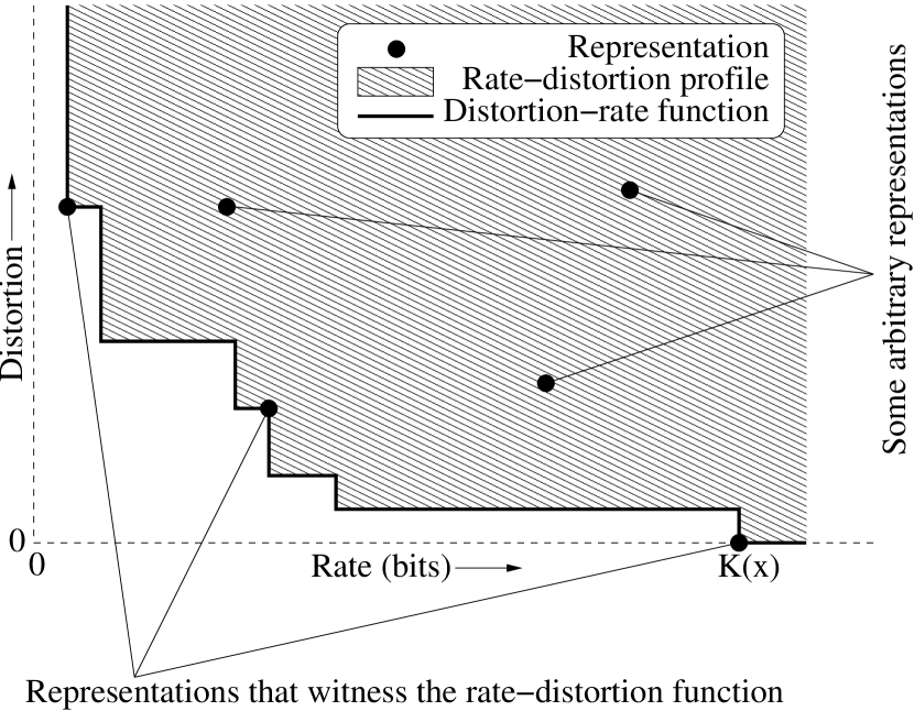The lack of fidelity of a representation $y$ is quantified by a distortion function $d:\mathcal{X}\times\mathcal{Y}\rightarrow\mathbb{R}$ .

The Kolmogorov complexity of $y$ , denoted $K(y)$ , is the length of the shortest program that constructs $y$ . More precisely, it is the length of the shortest input to a fixed universal binary prefix machine that will output $y$ and then halt; also see the textbook[LiVitanyi1997]. We can transmit any representation $y$ that has $K(y)\leq r$ , the receiver can then run the program to obtain $y$ and is thus able to reconstruct $x$ up to distortion $d(x,y)$ . Define the rate-distortion profile $P_{x}$ of the source word $x$ as the set of pairs $\left\langle r,a\right\rangle$ such that there is a representation $y\in\mathcal{Y}$ with $d(x,y)\leq a$ and $K(y)\leq r$ . The possible combinations of $r$ and $a$ can also be characterised by the rate-distortion function of the source word $x$ , which is defined as $r_{x}(a)=\min\{r:\left\langle r,a\right\rangle\in P_{x}\}$ , or by the distortion-rate function of the source word $x$ , which is defined as $d_{x}(r)=\min\{a:\left\langle r,a\right\rangle\in P_{x}\}$ . These two functions are somewhat like inverses of each other; although strictly speaking they are not since they are monotonic but not strictly monotonic. A representation $y$ is said to witness the rate-distortion function of $x$ if $r_{x}(d(x,y))=K(y)$ . These definitions are illustrated in Figure 1.

Algorithmic rate-distortion theory is developed and treated in much more detail in [VereshchaginVitanyi2005]. It is a generalization of Kolmogorov’s structure function theory, see [VereshchaginVitanyi2004].

Refer to caption — Figure 1: Rate-distortion profile and distortion-rate function

II-A Side Information

We generalize the algorithmic rate-distortion framework, so that it can accommodate side information. Suppose that we want to transmit a source word $x\in\mathcal{X}$ and we have chosen a representation $y\in\mathcal{Y}$ as before. The encoder and decoder often share a lot of information: both might know that grass is green and the sky is blue, they might share a common language, and so on. They would not need to transmit such information. If encoder and decoder share some information $z$ , then the programs they transmit to compute the representation $y$ may use this side information $z$ . Such programs might be shorter than they could be otherwise. This can be formalised by switching to the conditional Kolmogorov complexity $K(y|z)$ , which is the length of the shortest Turing machine program that constructs $y$ on input $z$ . We redefine $K(y)=K(y|\epsilon)$ , where $\epsilon$ is the empty sequence, so that $K(y|z)\leq K(y)+O(1)$ : the length of the shortest program for $y$ can never significantly increase when side information is provided, but it might certainly decrease when $y$ and $z$ share a lot of information[LiVitanyi1997]. We change the definitions as follows: The rate-distortion profile of the source word $x$ with side information $z$ is the set of pairs $\left\langle r,a\right\rangle$ such that there is a representation $y\in\mathcal{Y}$ with $d(x,y)\leq a$ and $K(y|z)\leq r$ . The definitions of the rate-distortion function and the distortion-rate function are similarly changed. Henceforth we will omit mention of the side information $z$ unless it is relevant to the discussion.

While this generalization seems very natural the authors are not aware of earlier proposals along these lines. In Section V we will demonstrate one use for this generalized rate-distortion theory: removal of spelling errors in written text, an example where denoising is not practical without use of side information.

II-B Distortion Spheres and the Minimal Sufficient Statistic

A representation $y$ that witnesses the rate-distortion function is the best possible rendering of the source object $x$ at the given rate because it minimizes the distortion, but if the rate is lower than $K(x)$ , then some information is necessarily lost. Since one of our goals is to find the best possible separation between structure and noise in the data, it is important to determine to what extent the discarded information is noise.

Given a representation $y$ and the distortion $a=d(x,y)$ , we can find the source object $x$ somewhere on the list of all $x^{\prime}\in\mathcal{X}$ that satisfy $d(x^{\prime},y)=a$ . The information conveyed about $x$ by $y$ and $a$ is precisely, that $x$ can be found on this list. We call such a list a distortion sphere. A distortion sphere of radius $a$ , centred around $y$ is defined as follows:

S_{y}(a):=\{x^{\prime}\in\mathcal{X}:d(x^{\prime},y)=a\}.

(1)

If the discarded information is pure white noise, then this means that $x$ must be a completely random element of this list. Conversely, all random elements in the list share all “simply described” (in the sense of having low Kolmogorov complexity) properties that $x$ satisfies. Hence, with respect to the “simply described” properties, every such random element is as good as $x$ , see [VereshchaginVitanyi2005] for more details. In such cases a literal specification of the index of $x$ (or any other random element) in the list is the most efficient code for $x$ , given only that it is in $S_{y}(a)$ . A fixed-length, literal code requires $\log|S_{y}(a)|$ bits. (Here and in the following, all logarithms are taken to base $2$ unless otherwise indicated.) On the other hand, if the discarded information is structured, then the Kolmogorov complexity of the index of $x$ in $S_{y}(a)$ will be significantly lower than the logarithm of the size of the sphere. The difference between these two codelengths can be used as an indicator of the amount of structural information that is discarded by the representation $y$ . Vereshchagin and Vitányi[VereshchaginVitanyi2005] call this quantity the randomness deficiency of the source object $x$ in the set $S_{y}(a)$ , and they show that if $y$ witnesses the rate-distortion function of $x$ , then it minimizes the randomness deficiency at rate $K(y)$ ; thus the rate-distortion function identifies those representations that account for as much structure as possible at the given rate.

To assess how much structure is being discarded at a given rate, consider a code for the source object $x$ in which we first transmit the shortest possible program that constructs both a representation $y$ and the distortion $d(x,y)$ , followed by a literal, fixed-length index of $x$ in the distortion sphere $S_{y}(a)$ . Such a code has the following length function:

L_{y}(x):=K(\left\langle y,d(x,y)\right\rangle)+\log|S_{y}(d(x,y))|.

(2)

If the rate is very low then the representation $y$ models only very basic structure and the randomness deficiency in the distortion sphere around $y$ is high. Borrowing terminology from statistics, we may say that $y$ is a representation that “underfits” the data. In such cases we should find that $L_{y}(x)>K(x)$ , because the fixed-length code for the index of $x$ within the distortion sphere is suboptimal in this case. But suppose that $y$ is complex enough that it satisfies $L_{y}(x)\approx K(x)$ . In [VereshchaginVitanyi2005], such representations are called (algorithmic) sufficient statistics for the data $x$ . A sufficient statistic has close to zero randomness deficiency, which means that it represents all structure that can be detected in the data. However, sufficient statistics might contain not only structure, but noise as well. Such a representation would be overly complex, an example of overfitting. A minimal sufficient statistic balances between underfitting and overfitting. It is defined as the lowest complexity sufficient statistic, which is the same as the lowest complexity representation $y$ that minimizes the codelength $L_{y}(x)$ . As such it can also be regarded as the “model” that should be selected on the basis of the Minimum Description Length (MDL) principle[BarronRY98]. To be able to relate the distortion-rate function to this codelength we define the codelength function $\lambda_{x}(r)=L_{y}(x)$ where $y$ is the representation that minimizes the distortion at rate $r$ .¹¹1This is superficially similar to the MDL function defined in [VereshchaginVitanyi2004], but it is not exactly the same since it involves optimisation of the distortion at a given rate rather than direct optimisation of the code length.

II-C Applications: Denoising and Lossy Compression

Representations that witness the rate-distortion function provide optimal separation between structure that can be expressed at the given rate and residual information that is perceived as noise Therefore, these representations can be interpreted as denoised versions of the original. In denoising, the goal is of course to discard as much noise as possible, without losing any structure. Therefore the minimal sufficient statistic, which was described in the previous section, is the best candidate for applications of denoising.

While the minimum sufficient statistic is a denoised representation of the original signal, it is not necessarily given in a directly usable form. For instance, $\mathcal{Y}$ could consist of subsets of $\mathcal{X}$ , but a set of source-words is not always acceptable as a denoising result. So in general one may need to apply some function $f:\mathcal{Y}\rightarrow\mathcal{X}$ to the sufficient statistic to construct a usable object. But if $\mathcal{X}=\mathcal{Y}$ and the distortion function is a metric, as in our case, then the representations are already in an acceptable format, so here we use the identity function for the transformation $f$ .

In applications of lossy compression, one may be willing to accept a rate which is lower than the minimal sufficient statistic complexity, thereby losing some structural information. However, for a minimal sufficient statistic $y$ , theory does tell us that it is not worthwhile to set the rate to a higher value than the complexity of $y$ . The original object $x$ is a random element of $S_{y}(d(x,y))$ , and it cannot be distinguished from any other random $z\in S_{y}(d(x,y))$ using only “simply described” properties. So we have no “simply described” test to discredit the hypothesis that $x$ (or any such $z$ ) is the original object, given $y$ and $d(x,y)$ . But increasing the rate, yielding a model $y^{\prime}$ and $d(x,y^{\prime})<d(x,y)$ , we commonly obtain a sphere $S_{y^{\prime}}$ of smaller cardinality than $S_{y}$ , with some random elements of $S_{y}$ not being random elements of $S_{y^{\prime}}$ . These excluded elements, however, were perfectly good candidates of being the original object. That is, at rate higher than that of the minimal sufficient statistic, the resulting representation $y^{\prime}$ models irrelevant features that are specific to $x$ , that is, noise and no structure, that exclude viable candidates for the olriginal object: the representation starts to “overfit”.

In lossy compression, as in denoising, the representations themselves may be unsuitable for presentation to the user. For example, when decompressing a lossily compressed image, in most applications a set of images would not be an acceptable result. So again a transformation from representations to objects of a usable form has to be specified. There are two obvious ways of doing this:

1.

If a representation $y$ witnesses the rate-distortion function for a source word $x\in\mathcal{X}$ , then this means that $x$ cannot be distinguished from any other object $x^{\prime}\in S_{y}(d(x,y))$ at rate $K(y)$ . Therefore we should not use a deterministic transformation, but rather report the uniform distribution on $S_{y}(d(x,y))$ as the lossily compressed version of $x$ . This method has the advantage that it is applicable whether or not $\mathcal{X}=\mathcal{Y}$ .
2.

On the other hand, if $\mathcal{X}=\mathcal{Y}$ and the distortion function is a metric, then it makes sense to use the identity transformation again, although here the motivation is different. Suppose we select some $x^{\prime}\in S_{y}(d(x,y))$ instead of $y$ . Then the best upper bound we can give on the distortion is $d(x,x^{\prime})\leq d(x,y)+d(y,x^{\prime})=2d(x,y)$ (by the triangle inequality and symmetry). On the other hand if we select $y$ , then the distortion is exactly $d(x,y)$ , which is only half of the upper bound we obtained for $x^{\prime}$ . Therefore it is more suitable if one adopts a worst-case approach. This method has as an additional advantage that the decoder does not need to know the distortion $d(x,y)$ which often cannot be computed from $y$ without knowledge of $x$ .

To illustrate the difference one may expect from these approaches, consider the situation where the rate is lower than the rate that would be required to specify a sufficient statistic. Then intuitively, all the noise in the source word $x$ as well as some of the structure are lost by compressing it to a representation $y$ . The second method immediately reports $y$ , which contains a lot less noise than the source object $x$ ; thus $x$ and $y$ are qualitatively different, which may be undesirable. On the other hand, the compression result will be qualitatively different from $x$ anyway, because the rate simply is too low to retain all structure. If one would apply the first approach, then a result $x^{\prime}$ would likely contain more noise than the original, because it contains less structure at the same level of distortion (meaning that $K(x^{\prime})>K(x)$ while $d(x^{\prime},y)=d(x,y)$ ).

If the rate is high enough to transmit a sufficient statistic, then the first approach seems preferable. We have nevertheless chosen to always report $y$ directly in our analysis, which has the advantage that this way, all reported results are of the same type.

III Computing Individual Object Rate-Distortion

The rate-distortion function for an object $x$ with side information $z$ and a distortion function $d$ is found by simultaneous minimizing two objective functions

$\displaystyle g_{1}(y)$	$\displaystyle=$	$\displaystyle K(y\|z)$	(3)
$\displaystyle g_{2}(y)$	$\displaystyle=$	$\displaystyle d(x,y)$	(4)
$\displaystyle g(y)$	$\displaystyle=$	$\displaystyle\left\langle g_{1}(y),g_{2}(y)\right\rangle.$

We call the tuple $g(y)$ the trade-off of $y$ . We impose a partial order on representations:

y\preccurlyeq y^{\prime}

(5)

if and only if $g_{1}(y)\leq g_{1}(y^{\prime})$ and $g_{2}(y)\leq g_{2}(y^{\prime})$ . Our goal is to find the set of Pareto-optimal representations, that is, the set of representations that are minimal under $\preccurlyeq$ .

Such an optimisation problem cannot be implemented because of the uncomputability of $K(\cdot)$ . To make the idea practical, we need to approximate the conditional Kolmogorov complexity. As observed in [VitanyiCilibrasi2004], it follows directly from symmetry of information for Kolmogorov complexity (see [LiVitanyi1997, p.233]) that:

K(y|z)=K(zy)-K(z)+O(\log n),

(6)

where $n$ is the length of $zy$ . Ignoring the logarithmic term, this quantity can be approximated by replacing $K(\cdot)$ by the length of the compressed representation under a general purpose compression algorithm $A:\mathcal{X}\rightarrow\{0,1\}^{*}$ . The length of the compressed representation of $x$ is denoted by $L_{A}(x)$ . This way we obtain, up to an additive independent constant:

K(y|z)\leq L_{A}(zy)-L_{A}(z).

(7)

We redefine $g_{1}(y):=L_{A}(zy)-L_{A}(z)$ in order to get a practical objective function.

This may be a poor approximation: we only have that $0\leq K(y|z)\leq L_{A}(zy)-L_{A}(z)$ , up to a constant, so the compressed size is an upper bound that may be quite high even for objects that have Kolmogorov complexity close to zero. Our results show evidence that some of the theoretical properties of the distortion-rate function nevertheless carry over to the practical setting; we also explain how some observations that are not predicted by theory are in fact related to the (unavoidable) inefficiencies of the used compressor.

III-A Compressor (rate function)

We could have used any general-purpose compressor in (7), but we chose to implement our own for three reasons:

•

It should be both fast and efficient. We can gain some advantage over other available compressors because there is no need to actually construct a code. It suffices to compute code lengths, which is much easier. As a secondary advantage, the codelengths we compute are not necessarily multiples of eight bits: we allow rational idealised codelengths, which may improve precision.
•

It should not have any arbitrary restrictions or optimisations. Most general purpose compressors have limited window sizes or optimisations to improve compression of common file types; such features could make the results harder to interpret.

In our experiments we used a block sorting compression algorithm with a move-to-front scheme as descibed in [burrowswheeler1994]. In the encoding stage M2 we employ a simple statistical model and omit the actual encoding as it suffices to accumulate codelengths. The source code of our implementation (in C) is available from the authors upon request. The resulting algorithm is very similar to a number of common general purpose compressors, such the freely available bzip2[bzip2] and zzip[zzip], but it is simpler and faster for small inputs.

Of course, domain specific compressors might yield better compression for some object types (such as sound wave files), and therefore a better approximation of the Kolmogorov complexity. However, the compressor that we implemented is quite efficient for objects of many of the types that occur in practice; in particular it compressed the objects of our experiments (text and small images) quite well. We have tried to improve compression performance by applying standard image preprocessing algorithms to the images, but this turned out not to improve compression at all. Figure 2 lists the compressed size of an image of a mouse under various different compression and filtering regimes. Compared to other compressors, ours is quite efficient; this is probably because other compressors are optimised for larger files and because we avoid all overhead inherent in the encoding process. Most compressors have optimisations for text files which might explain why our compressor compares less favourably on the Oscar Wilde fragment.

Compression	mouse	cross	Wilde	description
A	7995.11	3178.63	3234.45	Our compressor, described in §III-A
zzip	8128.00	3344.00	3184.00	An efficient block sorting compressor
PPMd	8232.00	2896.00	2744.00	High end statistical compressor
RLE $\rightarrow$ A	8341.68	3409.22	–	A with run length encoding filter
bzip2	9296.00	3912.00	3488.00	Widespread block sorting compressor
gzip	9944.00	4008.00	3016.00	LZ77 compressor
sub $\rightarrow$ A	10796.29	4024.26	–	A with Sub filter
paeth $\rightarrow$ A	13289.34	5672.70	–	A with Paeth filter
None	20480.00	4096.00	5864.00	Literal description

Figure 2: Compressed sizes of three objects that we experiment upon. See Figure 5 for the mouse, Figure 6 for the cross with added noise and Figure LABEL:fig:dorian_gray for the corrupted Oscar Wilde fragment (the middle version). In the latter we give the compressed size conditional on a training text, like in the experiments. “A” is our own algorithm, described in Section III-A. For a description of the filters see [OReillyPNG].

III-B Codelength Function

In Section II-B we introduced the codelength function $\lambda_{x}(r)$ . Its definition makes use of (2), for which we have not yet provided a computable alternative. We use the following approximation:

L_{y}(x)\approx L^{\prime}_{y}(x)=L_{A}(y)+L_{D}(d(x,y)|y)+L_{U}(x|y,d(x,y)),

(8)

where $L_{D}$ is yet another code which is necessary to specify the radius of the distortion sphere around $y$ in which $x$ can be found. It is possible that this distortion is uniquely determined by $y$ , for example if $\mathcal{Y}$ is the set of all finite subsets of $\mathcal{X}$ and list decoding distortion is used, as described in [VereshchaginVitanyi2004]. If $d(x,y)$ is a function of $y$ then $L_{D}(d(x,y)|y)=0$ . In other cases, the representations do not hold sufficient information to determine the distortion. This is typically the case when $\mathcal{X}=\mathcal{Y}$ as in the examples in this text. In that case we actually need to encode $d(x,y)$ separately. It turns out that the number of bits that are required to specify the distortion are negligible in proportion to the total three part codelength. In the remainder of the paper we use for $L_{D}$ a universal code on the integers similar to the one described in [LiVitanyi1997]; it has codelength $L_{D}(d)=\log(d+1)+O(\log\log d)$ .

III-C Distortion Functions

We use three common distortion functions which we describe below. All distortion functions used in this text are metrics, which have the property that $\mathcal{X}=\mathcal{Y}$ .

Hamming distortion

Hamming distortion is perhaps the simplest distortion function that could be used. Let $x$ and $y$ be two objects of equal length $n$ . The Hamming distortion $d(x,y)$ is equal to the number of symbols in $x$ that do not match those in the corresponding positions in $y$ .

Euclidean distortion

As before, let $x=x_{1}\ldots x_{n}$ and $y=y_{1}\ldots y_{n}$ be two objects of equal length, but the symbols now have a numerical interpretation. Euclidean distortion is $d(x,y)=\sqrt{\sum_{i=1}^{n}(x_{i}-y_{i})^{2}}$ : the distance between $x$ and $y$ when they are interpreted as vectors in an $n$ -dimensional Euclidean space. Note that this definition of Euclidean distortion differs from the one in [VereshchaginVitanyi2005].

Edit distortion

The edit distortion of two strings $x$ and $y$ , of possibly different lengths, is the minimum number of symbols that have to be deleted from, inserted into, or changed in $x$ in order to obtain $y$ (or vice versa)[Levenshtein1966]. It is also known as Levenshtein distortion. It is a well-known measure that is often used in applications that require approximate string matching.

III-D Searching for the Rate-Distortion Function

The search problem that we propose to address has two properties that make it very hard. Firstly, the search space is enormous: for an object of $n$ bits there are $2^{n}$ candidate representations of the same size, and objects that are typically subjected to lossy compression are often millions or billions of bits long. Secondly, we want to avoid making too many assumptions about the two objective functions, so that we can later freely change the compression algorithm and the distortion function. Under such circumstances the two most obvious search methods are not practical:

•

An exhaustive search is infeasible for search spaces of such large size, unless more specific properties of the objective functions are used in the design of the algorithm. To investigate how far we could take such an approach, we have implemented an exhaustive algorithm under the requirement that, given a prefix of a representation $y$ , we can compute reasonable lower bounds on the values of both objective functions $g_{1}$ and $g_{2}$ . This allows for relatively efficient enumeration of all representations of which the objective functions do not exceed specific maxima: it is never necessary to consider objects which have a prefix for which the lower bounds exceed the constraints, which allows for significant pruning. In this fashion we were able to find the rate-distortion function under Hamming distortion for objects of which the compressed size is about 25 bits or less within a few hours on a desk-top computer.
•

A greedy search starts with a poor solution and iteratively makes modifications that constitute strict improvements. We found that this procedure tends to terminate quickly in some local optimum that is very bad globally.

Since the structure of the search landscape is at present poorly understood and we do not want to make any unjustifiable assumptions, we use a genetic search algorithm which performs well enough that interesting results can be obtained. It is described in the Appendix LABEL:sect.ga.

IV Experiments

We have subjected four objects to our program. The following considerations have influenced our choice of objects:

•

Objects should not be too complex, allowing our program to find a good approximation of the distortion-rate curve. We found that the running time of the program seems to depend mostly on the complexity of the original object; a compressed size of 20,000 bits seemed to be about the maximum our program could handle within a reasonable amount of time, requiring a running time of the order of weeks on a desk-top computer.
•

To check that our method really is general, objects should be quite different: they should come from different object domains, for which different distortion functions are appropriate, and they should contain structure at different levels of complexity.
•

Objects should contain primary structure and regularities that are distinguishable and compressible by a block sorting compressor such as the one we use. Otherwise, we may no longer hope that the compressor implements a significant approximation of the Kolmogorov complexity. For instance, we would not expect our program to do well on a sequence of digits from the binary expansion of the number $\pi$ .

With this in mind, we have selected the objects listed in Figure 3.

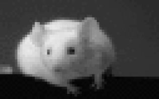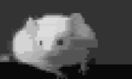
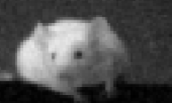
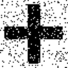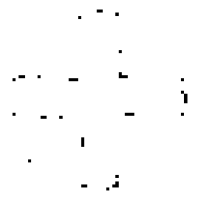
	A picture of a mouse of $64\times 40$ pixels. The picture is analyzed with respect to Euclidean distortion.		A noisy monochrome image of $64\times 64$ pixels that depicts a cross. 377 pixels have been inverted. Hamming distortion is used.
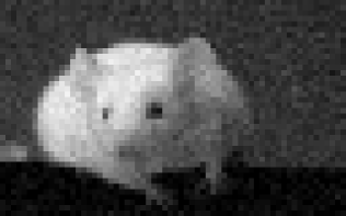	The same picture of a mouse, but now zero mean Gaussian noise with $\sigma=8$ has been added to each pixel. Euclidean distortion is used; the distortion to the original mouse is $391.1$ .	Beauty, real beauty, ends2wheresan intellectual expressoon begins. IntellHct isg in itself a mMde ofSexggeration, an $\backslash$ destroys theLharmony of n face. […] (See Figure LABEL:fig:dorian_gray)	A corrupted quotation from Chapter 1 of The Picture of Dorian Gray, by Oscar Wilde. The 733 byte long fragment was created by performing 68 random insertions, deletions and replacements of characters in the original text. Edit distortion is used. The rest of chapters one and two of the novel are given to the program as side information.

In each experiment, as time progressed the program in Appendix LABEL:sect.ga found less and less improvements per iteration, but the set of candidate solutions, called the pool in the Appendix, never stabilized completely. Therefore we interrupted each experiment when (a) after at least one night of computation, the pool did not improve a lot, and (b) for all intuitively good models $y\in\mathcal{Y}$ that we could conceive of a priori, the algorithm had found an $y^{\prime}$ in the pool with $y^{\prime}\preccurlyeq y$ according to (5). For example, in each denoising experiment, this test included the original, noiseless object. In the experiment on the mouse without added noise, we also included the images that can be obtained by reducing the number of grey levels in the original with an image manipulation program. Finally for the greyscale images we included a number of objects that can be obtained by subjecting the original object to JPEG2000 compression at various quality levels.

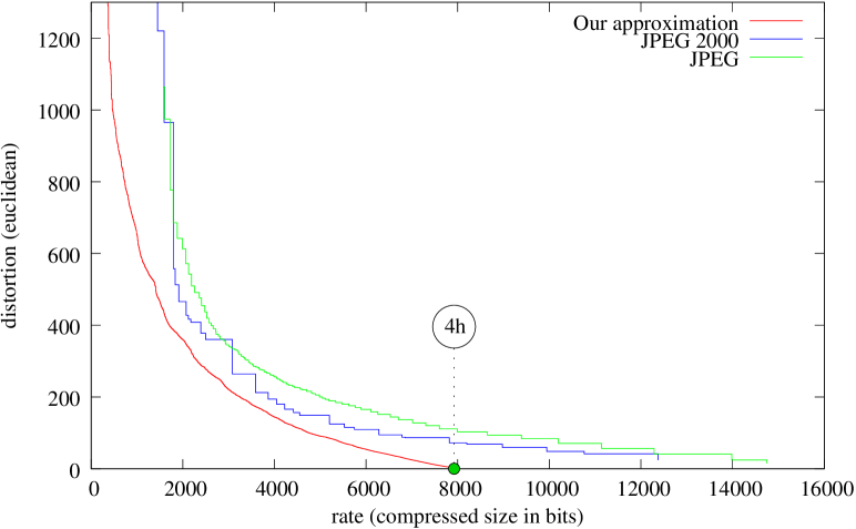
The first experiment illustrates how algorithmic rate-distortion theory may be applied to lossy compression problems, and it illustrates how for a given rate, some features of the image are preserved while others can no longer be retained. We compare the performance of our method to the performance of JPEG and JPEG2000 at various quality levels. Standard JPEG images were encoded using the ImageMagick version 6.2.2; profile information was stripped. JPEG2000 images were encoded to jpc format with three quality levels using NetPBM version 10.33.0; all other options are default. For more information about these software packages refer to [ImageMagick] and [NetPBM].

The other three experiments are concerned with denoising. Any model that is output by the program can be interpreted as a denoised version of the input object. We measure the denoising success of a model $y$ as $d(x^{\prime},y)$ , where $x^{\prime}$ is the original version of the input object $x$ , before noise was added. We also compare the denoising results to those of other denoising algorithms:

1.

BayesShrink denoising[Chang2000]. BayesShrink is a popular wavelet-based denoising method that is considered to work well for images.
2.

Blurring (convolution with a Gaussian kernel). Blurring works like a low-pass filter, eliminating high frequency information such as noise. Unfortunately other high frequency features of the image, such as sharp contours, are also discarded.
3.

Naive denoising. We applied a naive denoising algorithm to the noisy cross, in which each pixel was inverted if five or more out of the eight neighbouring pixels were of different colour.
4.

Denoising based on JPEG2000. Here we subjected the noisy input image to JPEG2000 compression at different quality levels. We then selected the result for which the distortion to the original image was lowest.

IV-A Names of Objects

To facilitate description and discussion of the experiments we will adopt the following naming convention. Objects related to the experiments with the mouse, the noisy cross, the noisy mouse and the Wilde fragment, are denoted by the symbols $\mathbb{M}$ , $\mathbb{C}$ , $\mathbb{N}$ and $\mathbb{W}$ respectively. A number of important objects in each experiment are identified by a subscript as follows. For $\mathbb{O}\in\{\mathbb{M},\mathbb{C},\mathbb{N},\mathbb{W}\}$ , the input object, for which the rate-distortion function is approximated by the program, is called $\mathbb{O}_{\textsc{\footnotesize in}}$ , which is sometimes abbreviated to $\mathbb{O}$ . In the denoising experiments, the input object is always constructed by adding noise to an original object. The original objects and the noise are called $\mathbb{O}_{\textsc{\footnotesize orig}}$ and $\mathbb{O}_{\textsc{\footnotesize noise}}$ respectively. If Hamming distortion is used, addition is carried out modulo 2, so that the input object is in effect a pixelwise exclusive OR of the original and the noise. In particular, $\mathbb{C}_{\textsc{\footnotesize in}}$ equals $\mathbb{C}_{\textsc{\footnotesize orig}}$ XOR $\mathbb{C}_{\textsc{\footnotesize noise}}$ . The program outputs the reduction of the gene pool, which is the set of considered models. Two important models are also given special names: the model within the gene pool that minimizes the distortion to $\mathbb{O}_{\textsc{\footnotesize orig}}$ constitutes the best denoising of the input object and is therefore called $\mathbb{O}_{\textsc{\footnotesize best}}$ , and the minimal sufficient statistic as described in Section II-B is called $\mathbb{O}_{\textsc{\footnotesize mss}}$ . Finally, in the denoising experiments we also give names to the results of the alternative denoising algorithms. Namely, $\mathbb{C}_{\textsc{\footnotesize naive}}$ is the result of the naive denoising algorithm applied to the noisy cross, $\mathbb{N}_{\textsc{\footnotesize blur}}$ is the convolution of $\mathbb{N}$ with a Gaussian kernel with $\sigma=0.458$ , $\mathbb{N}_{\textsc{\footnotesize bs}}$ is the denoising result of the BayesShrink algorithm, and $\mathbb{N}_{\textsc{\footnotesize jpeg2000}}$ is the image produced by subjecting $\mathbb{N}$ to JPEG2000 compression at the quality level for which the distortion to $\mathbb{N}_{\textsc{\footnotesize orig}}$ is minimized.

V Results and Discussion

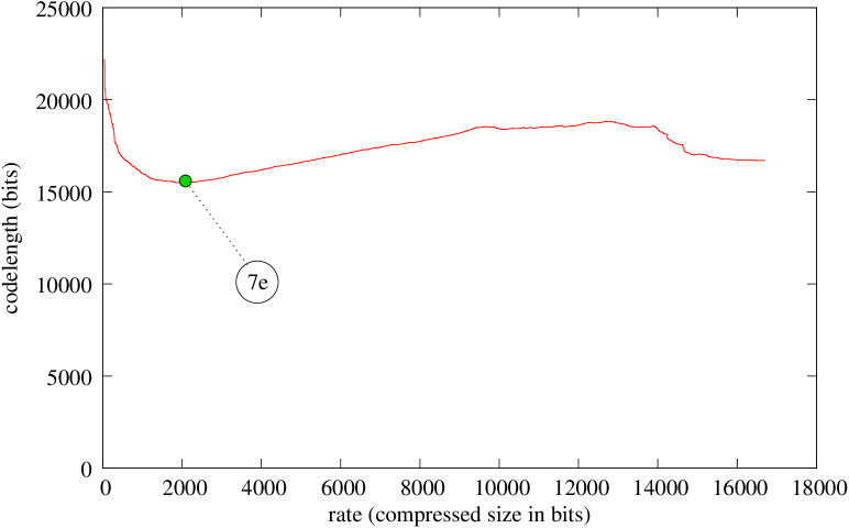
We will occasionally use terminology from Appendix LABEL:sect.ga, but such references can safely be glossed over on first reading. After running for some time on each input object, our program outputs the reduction of a pool $\mathcal{P}$ , which is interpreted as a set of models. For each experiment, we report a number of different properties of these sets. Since we are interested in the rate-distortion properties of the input object $x=\mathbb{O}_{\textsc{\footnotesize in}}$ , we plot the approximation of the distortion-rate function of each input object: $d_{x}(r)=\min\{d(x,y):y\in\mathcal{Y},K(y)\leq r\}\approx\min\{d(x,y):y\in\hbox{trd}(\mathcal{P}),L_{A}(y)\leq r\}$ , where $L_{A}$ denotes the codelength for an object under our compression algorithm. Such approximations of the distortion-rate function are provided for all four experiments. For the greyscale images we also plot the distortion-rate approximation that is achieved by JPEG2000 (and in Figure 5 also ordinary JPEG) at different quality levels. Here, the rate is the codelength achieved by JPEG(2000), and the distortion is the Euclidean distortion to $\mathbb{O}_{\textsc{\footnotesize in}}$ . We also plot the codelength function as discussed in Section II-B. Minimal sufficient statistics can be identified by locating the minimum of this graph.

V-A Lossy Compression

Experiment 1: $\mathbb{M}$ ouse (Euclidean distortion)

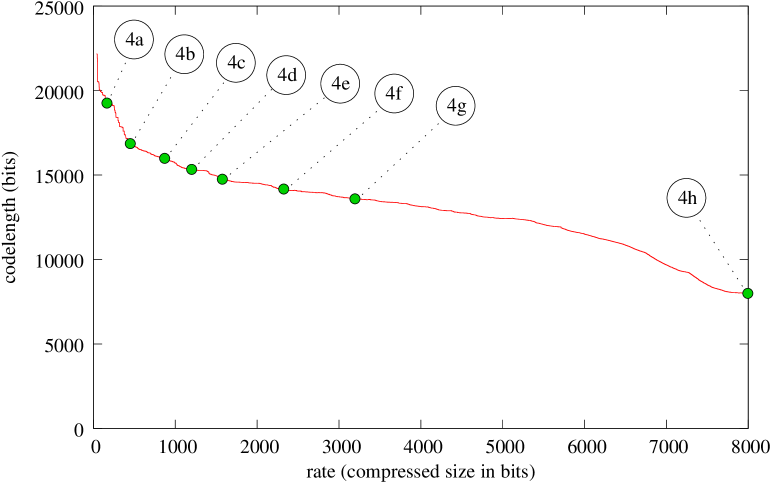
Our first experiment involved the lossy compression of $\mathbb{M}$ , a greyscale image of a mouse. A number of elements of the gene pool are shown in Figure 4. The pictures show how at low rates, the models capture the most important global structures of the image; at higher rates more subtle properties of the image can be represented. Figure 4(a) shows a rough rendering of the distribution of bright and dark areas in $\mathbb{M}_{\textsc{\footnotesize in}}$ . These shapes are rectangular, which is probably an artifact of the compression algorithm we used: it is better able to compress images with rectangular structure than with circular structure. There is no real reason why a circular structure should be in any way more complex than a rectangular structure, but most general purpose data compression software is similarly biased. In 4(b), the rate is high enough that the oval shape of the mouse can be accommodated, and two areas of different overall brightness are identified. After the number of grey shades has been increased a little further in 4(c), the first hint of the mouse’s eyes becomes visible. The eyes are improved and the mouse is given paws in 4(d). At higher rates, the image becomes more and more refined, but the improvements are subtle and seem of a less qualitative nature.

Figure 5(b) shows that the only sufficient statistic in the set of models is $\mathbb{M}_{\textsc{\footnotesize in}}$ itself, indicating that the image hardly contains any noise. It also shows the rates that correspond to the models that are shown in Figure 4. By comparing these figures it can be clearly seen that the image quality only starts to deteriorate significantly after more than half of the information in $\mathbb{M}_{\textsc{\footnotesize in}}$ has been discarded. Note that this is not a statement about the compression ratio, where the size is related to the size of the uncompressed object. For example, $\mathbb{M}_{\textsc{\footnotesize in}}$ has an uncompressed size of $64\cdot 40\cdot 8=20480$ bits, and the representation in Figure 4(g) has a compressed size of $3190.6$ bits. This representation therefore constitutes compression by a factor of $20480/3190.6=6.42$ , which is substantial for an image of such small size. At the same time the amount of information is reduced by a factor of $7995.0/3190.6=2.51$ .

V-B Denoising

For each denoising experiment, we report a number of important objects, a graph that shows the approximate distortion-rate function and a graph that shows the approximate codelength function. In the distortion-rate graph we plot not only the distortion to $\mathbb{O}_{\textsc{\footnotesize in}}$ but also the distortion to $\mathbb{O}_{\textsc{\footnotesize orig}}$ , to visualise the denoising success at each rate.

In interpreting these results, it is important to realise that only the reported minimal sufficient statistic and the results of the BayesShrink and naive denoising methods can be obtained without knowledge of the original object – the other objects $\mathbb{O}_{\textsc{\footnotesize best}}$ , $\mathbb{O}_{\textsc{\footnotesize jpeg2000}}$ and $\mathbb{O}_{\textsc{\footnotesize blur}}$ require selecting between a number of alternatives in order to optimise the distortion to $\mathbb{O}_{\textsc{\footnotesize orig}}$ , which can only be done in a controlled experiment. Their performance may be better than what can be achieved in practical situations where $\mathbb{O}_{\textsc{\footnotesize orig}}$ is not known.

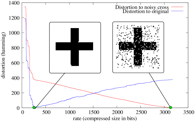
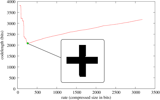
Experiment 2: Noisy $\mathbb{C}$ ross (Hamming distortion)

In the first denoising experiment we approximated the distortion-rate function of a monochrome cross $\mathbb{C}_{\textsc{\footnotesize orig}}$ of very low complexity, to which artificial noise was added to obtain $\mathbb{C}_{\textsc{\footnotesize in}}$ . Figure 6 shows the result; the distortion to the noiseless cross is displayed in the same graph. The best denoising $\mathbb{C}_{\textsc{\footnotesize best}}$ has a distortion of only $3$ to the original $\mathbb{C}_{\textsc{\footnotesize orig}}$ , which shows that the distortion-rate function indeed separates structure and noise extremely well in this example. Figure 6(b) shows the codelength function for the noisy cross; the minimum on this graph is the minimal sufficient statistic $\mathbb{C}_{\textsc{\footnotesize mss}}$ . In this low complexity example, we have $\mathbb{C}_{\textsc{\footnotesize mss}}=\mathbb{C}_{\textsc{\footnotesize best}}$ , so the best denoising is not only very good in this simple example, but it can also be identified.

We did not subject $\mathbb{C}$ to BayesShrink or blurring because those methods are unsuitable to monochrome images. Therefore we used the extremely simple, “naive” denoising method that is described in Section IV on this specific image instead. The result is shown in Figure 6(c); while it does remove most of the noise, 40 errors remain which is a lot more than those incurred by the minimal sufficient statistic. Figure 6(d) shows that all errors except one are close to the contours of the cross. This illustrates how the naive algorithm is limited by its property that it takes only the local neighbourhood of each pixel into account, it cannot represent larger structures such as straight lines.

Experiment 3: $\mathbb{N}$ oisy mouse (Euclidean distortion)

The noisy mouse poses a significantly harder denoising problem, where the total complexity of the input $\mathbb{N}_{\textsc{\footnotesize in}}$ is more than five times as high as for the noisy cross. The graphs that show the approximation to the distortion-rate function and the codelength function are in Figure 8, below we discuss the approximations that are indicated on the graphs with references to Figure 7.

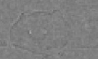
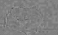
Figure 7(b) shows the input object $\mathbb{N}_{\textsc{\footnotesize in}}$ ; it was constructed by adding noise to the original noiseless image $\mathbb{N}_{\textsc{\footnotesize orig}}$ = $\mathbb{M}_{\textsc{\footnotesize in}}$ . We have displayed the denoising results which were obtained in three different ways. In Figure 7(c) we have shown $\mathbb{N}_{\textsc{\footnotesize best}}$ , the best denoised object from the gene pool. Visually it appears to resemble $\mathbb{N}_{\textsc{\footnotesize orig}}$ quite well, but it might be the case that there is structure in $\mathbb{N}_{\textsc{\footnotesize orig}}$ that is lost in the denoising process. Because human perception is perhaps the most sensitive detector of structure in image data, we have shown the difference between $\mathbb{N}_{\textsc{\footnotesize best}}$ and $\mathbb{N}_{\textsc{\footnotesize orig}}$ in Figure 7(d). We would expect any significant structure in the original image that is lost in the denoising process, as well as structure that is not present in the original image, but is somehow introduced as an artifact of the denoising procedure, to become visible in this residual image. In the case of $\mathbb{N}_{\textsc{\footnotesize best}}$ we cannot make out any particular features in the residual.

We have done the same for the minimal sufficient statistic (Figure 7(e)). The result also appears to be a quite successful denoising, although it is clearly of lower complexity than the best one. This is also visible in the residual, which still does not appear to contain much structure, but darker and lighter patches are definitely discernible. Apparently the difference between $\mathbb{N}_{\textsc{\footnotesize in}}$ and $\mathbb{N}_{\textsc{\footnotesize mss}}$ does contain some structure, but is nevertheless coded more efficiently using a literal description than using the given compression algorithm. We think that the fact that the minimal sufficient statistic is of lower complexity than the best possible denoising result should therefore again be attributed to inefficiencies of the compressor.

For comparison, we have also denoised $\mathbb{N}$ using the alternative denoising method BayesShrink and the methods based on blurring and JPEG2000 as described in Section IV. We found that BayesShrink does not work well for images of such small size: the distortion between $\mathbb{N}_{\textsc{\footnotesize bs}}$ and $\mathbb{N}_{\textsc{\footnotesize in}}$ is only 72.9, which means that the input image is hardly effected at all. Also, $\mathbb{N}_{\textsc{\footnotesize bs}}$ has a distortion of 383.8 to $\mathbb{N}_{\textsc{\footnotesize orig}}$ , which is hardly less than the distortion of 392.1 achieved by $\mathbb{N}_{\textsc{\footnotesize in}}$ itself.

(Continued after Figures 6–8.)

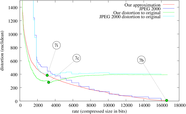
Blurring-based denoising yields much better results: $\mathbb{N}_{\textsc{\footnotesize blur}}$ is the result after optimisation of the size of the Gaussian kernel. Its distortion to $\mathbb{N}_{\textsc{\footnotesize orig}}$ lies in-between the distortions achieved by $\mathbb{N}_{\textsc{\footnotesize mss}}$ and $\mathbb{N}_{\textsc{\footnotesize best}}$ , but it is different from those objects in two important respects. Firstly, $\mathbb{N}_{\textsc{\footnotesize blur}}$ remains much closer to $\mathbb{N}_{\textsc{\footnotesize in}}$ , at a distortion of 260.4 instead of more than 470, and secondly, $\mathbb{N}_{\textsc{\footnotesize blur}}$ is much less compressible by $L_{A}$ . (To obtain the reported size of 14117 bits we had to switch on the averaging filter, as described in Section III-A.) These observations are at present not well understood. Figure 7(h) shows that the contours of the mouse are somewhat distorted in $\mathbb{N}_{\textsc{\footnotesize blur}}$ ; this can be explained by the fact that contours contain high frequency information which is discarded by the blurring operation as we remarked in Section IV.

The last denoising method we compared our results to is the one based on the JPEG2000 algorithm. Its performance is clearly inferior to our method visually as well as in terms of rate and distortion. The result seems to have undergone a smoothing process similar to blurring which introduces similar artifacts in the background noise, as is clearly visible in the residual image. As before, the comparison may be somewhat unfair because JPEG2000 was not designed for the purpose of denoising, might optimise a different distortion measure and is much faster.

Experiment 4: Oscar $\mathbb{W}$ ilde fragment (edit distortion)

The fourth experiment, in which we analyze $\mathbb{W}_{\textsc{\footnotesize in}}$ , a corrupted quotation from Oscar Wilde, shows that our method is a general approach to denoising that does not require many domain specific assumptions. $\mathbb{W}_{\textsc{\footnotesize orig}}$ , $\mathbb{W}_{\textsc{\footnotesize in}}$ and $\mathbb{W}_{\textsc{\footnotesize mss}}$ are depicted in Figure LABEL:fig:dorian_gray, the distortion-rate approximation, the distortion to $\mathbb{W}_{\textsc{\footnotesize orig}}$ and the three part codelength function are shown in Figure LABEL:fig:wilde. We have trained the compression algorithm by supplying it with the rest of Chapters 1 and 2 of the same novel as side information, to make it more efficient at compressing fragments of English text. We make the following observations regarding the minimal sufficient statistic:

•

In this experiment, $\mathbb{W}_{\textsc{\footnotesize mss}}=\mathbb{W}_{\textsc{\footnotesize best}}$ so the minimal sufficient statistic separates structure from noise extremely well here.
•

The distortion is reduced from 68 errors to only 46 errors. 26 errors are corrected ( $\blacktriangle$ ), 4 are introduced ( $\blacktriangledown$ ), 20 are unchanged ( $\bullet$ ) and 22 are changed incorrectly ( $\bigstar$ ).

•

The errors that are newly introduced ( $\blacktriangledown$ ) and the incorrect changes ( $\bigstar$ ) typically simplify the fragment a lot, so that the compressed size may be expected to drop significantly. Not surprisingly therefore, many of the symbols marked $\blacktriangledown$ or $\bigstar$ are deletions, or modifications that create a word which is different from the original, but still correct English. The following table lists examples of the last category:

Line	$\mathbb{W}_{\textsc{\footnotesize orig}}$	$\mathbb{W}_{\textsc{\footnotesize in}}$	$\mathbb{W}_{\textsc{\footnotesize mss}}$
3	or	Nor	of
3	the	Ghe	he
4	any	anL	an
4	learned	JeaFned	yearned
4	course	corze	core
5	then	ehen	when
7	he	fhe	the

Since it would be hard for any general-purpose mechanical method (that does not incorporate a specialized full linguistic model of English) to determine that these changes are incorrect, we should not be surprised to find a number of errors of this kind.

Side Information

Figure 9 shows that the compression performance is significantly improved if we provide side information to the compression algorithm, and the improvement is typically larger if (1) the amount of side information is larger, or (2) if the compressed object is more similar to the side information. Thus, by giving side information, correct English prose is recognised as “structure” sooner and a better separation between structure and noise is to be expected. The table also shows that if the compressed object is in some way different from the side information, then adding more side information will at some point become counter-productive, presumably because the compression algorithm will then use the side information to build up false expectations about the object to be compressed, which can be costly.

While denoising performance probably increases if the amount of side information is increased, it was infeasible to do so in this implementation. Recall from Section III that he conditional Kolmogorov complexity $K(y|z)$ is approximated by $L_{A}(zy)-L_{A}(z)$ . The time required to compute this is dominated by the length of $z$ if the amount of side information is much larger than the size of the object to be compressed. This could be remedied by using a compression algorithm $A^{\prime}$ that operates sequentially from left to right, because the state of such an algorithm can be cached after processing the side information $z$ ; computing $L_{A^{\prime}}(zy)$ would then be a simple matter of recalling the state that was reached after processing $z$ and then processing $y$ starting from that state. Many compression algorithms, among which Lempel-Ziv compressors and most statistical compressors, have this property; our approach could thus be made to work with large quantities of side information by switching to a sequential compressor but we have not done this.

Side information	$\!\!\!\!\!\!L_{A}(\mathbb{W}_{\textsc{\footnotesize orig}})$	$L_{A}(\mathbb{W}_{\textsc{\footnotesize mss}})$	$L_{A}(\mathbb{W}_{\textsc{\footnotesize in}})$
None	3344.1	3333.7	3834.8
Chapters 1,2 (57 kB)	1745.7	1901.9	3234.5
Whole novel (421 kB)	1513.6	1876.5	3365.9

Figure 9: Compressed size of models for different amounts of side information.

\mathbb{W}_{\textsc{\footnotesize orig}}

is never included in the side information. We do not let

\mathbb{W}_{\textsc{\footnotesize mss}}

vary with side information but keep it fixed at the object reported in Figure LABEL:fig:wilde_mdl.

Beauty, real beauty, ends where an intellectual expression begins. Intellect is in itself amode of exaggeration, and destroys the harmony of any face. The moment one sits down to think, one becomes all nose, or all forehead, or something horrid. Look at the successfulmen in any of the learned professions. How perfectly hideous they are! Except, of course, in the Church. But then in the Church they don’t think. A bishop keeps on saying at the ageof eighty what he was told to say when he was a boy of eighteen, and as a natural consequence he always looks absolutely delightful. Your mysterious young friend, whose name you have never told me, but whose picture really fascinates me, never thinks. I feel quite sure of that.

(a)

\mathbb{W}_{\textsc{\footnotesize orig}}

, the original text

Beauty, real beauty, ends2wheresan intellectual expressoon begins. IntellHct isg in itself a mMde ofSexggeration, an $\backslash$ destroys theLharmony of n face. :The m1ment one sits downto ahink@ one becomes jll noe^ Nor all forehbead, or something hNrrid. Look a Ghe successf $\backslash$ l men in anL of te JeaFned professions. How per}ectly tideous 4they re6 Except, of corze, in7 the Ch4rch. BuP ehen in the Church they dol’t bthink. =A bishop keeps on saying at the age of eighty what he was told to say wh”n he was aJb4y of eighten, and sja natural cnsequencefhe a(ways looks ab8olstely de[ightfu). Your mysterious youngL friend, wPose name you h $\backslash$ vo never tld me, mut whose picture really fa?scinates Lme,Pnever thinCs. I feel quite surS of that9

(b)

\mathbb{W}_{\textsc{\footnotesize in}}

, the corrupted version of the fragment. At 68 randomly selected positions characters have been inserted, deleted or modified. New and replacement characters are drawn uniformly from ASCII symbols 32–126.

Beauty, real beauty, ends