Optimal Design of Multiple Description Lattice Vector Quantizers

Abstract

In the design of multiple description lattice vector quantizers (MDLVQ), index assignment plays a critical role. In addition, one also needs to choose the Voronoi cell size of the central lattice $\nu$, the sublattice index $N$, and the number of side descriptions $K$ to minimize the expected MDLVQ distortion, given the total entropy rate of all side descriptions $R_{t}$ and description loss probability $p$. In this paper we propose a linear-time MDLVQ index assignment algorithm for any $K\geq 2$ balanced descriptions in any dimensions, based on a new construction of so-called $K$-fraction lattice. The algorithm is greedy in nature but is proven to be asymptotically ($N\to\infty$) optimal for any $K\geq 2$ balanced descriptions in any dimensions, given $R_{t}$ and $p$. The result is stronger when $K=2$: the optimality holds for finite $N$ as well, under some mild conditions. For $K>2$, a local adjustment algorithm is developed to augment the greedy index assignment, and conjectured to be optimal for finite $N$.

Our algorithmic study also leads to better understanding of $\nu$, $N$ and $K$ in optimal MDLVQ design. For $K=2$ we derive, for the first time, a non-asymptotical closed form expression of the expected distortion of optimal MDLVQ in $p$, $R_{t}$, $N$. For $K>2$, we tighten the current asymptotic formula of the expected distortion, relating the optimal values of $N$ and $K$ to $p$ and $R_{t}$ more precisely.

Key words: Lattices, multiple description vector quantization, index assignment, rate-distortion optimization.

I Introduction

Recent years have seen greatly increased research activities on multiple description coding (MDC), which are motivated by cooperative and distributed source coding for network communications. In a packet-switched network such as the Internet, an MDC-coded signal is transmitted in multiple descriptions (called side descriptions) via different routes from one or multiple servers to a receiver. Each side description can be independently decoded to reconstruct the signal at certain fidelity, while multiple side descriptions can be jointly decoded to reconstruct the signal at higher fidelity. By utilizing path diversity (the ability to communicate a content over different paths from a server to a client) and server diversity (the possibility of transmitting a source from multiple servers), MDC codes can weather adverse network conditions much better than single description codes, particularly in real-time communications where retransmission is not an option.

Multiple description codes can be generated by three categories of techniques: quantization, correlating transforms and erasure correction coding [1]. This paper is concerned with the approach of multiple description lattice vector quantization [2, 3, 4, 5, 6, 7, 8, 9, 10].

The first practical design of multiple description quantizer was the multiple description scaler quantizer (MDSQ) proposed by Vaishampayan in $1993$ [11]. The key mechanism of Vaishampayan’s technique is an index assignment (IA) scheme. In the case of two descriptions, the IA scheme labels each codeword of central quantizer by an ordered pair of indices, one for each side quantizer. MDSQ first quantizes a signal sample to a central quantizer codeword, then maps, via index assignment, this codeword to a pair of side quantizer indices. Vaishampayan proposed few index assignments for two-description balanced MDSQ [11]. These index assignments, although asymptotically good, were shown by Berger-Wolf and Reingold to be suboptimal [12]. The authors alternatively formulated MDSQ IA as a combinatorial optimization problem of arranging consecutive integers in a $K$-dimensional matrix similarly as in graph bandwidth problem [12]. With this formulation they proposed a constructive algorithm for MDSQ index assignment. The resulting index assignment was shown to minimize the maximum side distortion given central distortion, but only for a special case of two balanced description MDSQ when the index assignment matrix has no null elements (i.e., the number of central codewords is equal to the square of the number of side codewords, corresponding to having no redundancy in the system). Moreover, the technique of optimizing index assignment by arranging integers in a matrix cannot be extended to multiple description vector quantization (MDVQ), because no linear ordering of code vectors in two or higher dimensions can preserve spatial proximity.

Theoretically, MDVQ can achieve the MDC rate distortion bound as block length approaches infinity. Unfortunately, optimal MDVQ design is computationally intractable (optimal single-description VQ design is already NP-hard [13]). A practical way of managing the complexity is to use lattice VQ codebooks. This reduces the MDVQ design problem to one of choosing a lattice $\Lambda$ for central description and an associated sublattice $\Lambda_{s}$ for $K\geq 2$ side descriptions, and establishing a one-to-one mapping, called index assignment $\alpha$, between a point $\lambda\in\Lambda$ and an ordered $K$-tuple $(\lambda_{1},...,\lambda_{K})\in\Lambda_{s}^{K}$. The above MDVQ scheme was first proposed by Servetto et al. [2], and commonly referred to as multiple description lattice vector quantization (MDLVQ). Given the dimension of source vectors, lattices $\Lambda$ and $\Lambda_{s}$ can be selected from the known optimal and/or near-optimal lattice vector quantizers (e.g., those tabulated in [14]). Therefore, the key issue in optimal MDLVQ design is to find the bijection function $\alpha:\Lambda\leftrightarrow\alpha(\Lambda)\subset\Lambda_{s}^{K}$ that minimizes a distortion measure weighted over all possible channel/network scenarios.

The seminal paper of [4] studied the index assignment problem for $K=2$ balanced MDLVQ in considerable length, and proposed a “guiding principle” for constructing an optimal index assignment for two balanced descriptions. Also, the authors pointed out that optimal MDLVQ index assignment is a problem of linear assignment. However, a challenging algorithmic problem remains. This is how to reduce the graph matching problem from an association between two infinite sets $\Lambda$ and $\Lambda_{s}^{K}$ to between a finite subset of $\Lambda$ and a finite subset of $\Lambda_{s}^{K}$, and keep these two finite sets as small as possible without compromising optimality.

Diggavi et al. proposed a technique of converting the index assignment problem for two description lattice VQ to a finite bipartite graph matching problem [5]. Two sublattices $\Lambda_{1}$, $\Lambda_{2}$, and their product sublattice of $\Lambda_{s}$ are used to construct the two description LVQ. The index assignment is obtained by a minimum weight matching between a Voronoi set of central lattice points and a set of edges (ordered pairs of sublattice points, one end point in $\Lambda_{1}$ and the other in $\Lambda_{2}$). Each set has a cardinality of $N_{1}N_{2}$, where $N_{k}$ is the index of $\Lambda_{k}$, $k=1,2$. Therefore, the index assignment can be computed in $O((N_{1}N_{2})^{5/2})$ time, given that the weighted bipartite graph matching can be solved in $O(N^{5/2})$ time [15].

In [5] the authors only argued their index assignment algorithm to be optimal for two description lattice scalar quantizers, and left its optimality for lattice vector quantizers unexamined. This technique of constructing MDLVQ using a product sublattice was extended from two descriptions to any $K$ balanced descriptions by Østergaard et al. [10]. Østergaard et al. also used linear assignment to find index assignments. Their solution seemed to require $O(N^{5})$ time, where $N$ is the sublattice index, because it used a candidate set of $O(N^{2})$ central lattice points. Even with such a large set of candidate central lattice points, still no bound was given on the size of the candidate $K$-tuples of sublattice points used for labeling, and no proof of optimality was offered.

In this paper we propose an $O(N)$ greedy index assignment algorithm for MDLVQ of any $K\geq 2$ balanced descriptions in any dimensions. We prove that the algorithm minimizes the expected distortion given the loss probability $p$ and entropy rate $R_{s}$ of side descriptions, as $N\to\infty$. Moreover, for $K=2$, we can prove, under some mild conditions, the optimality of the algorithm for finite $N$ as well. For $K>2$ and a finite $N$, we augment the greedy algorithm by a fast local adjustment procedure, if necessary. We conjecture that this augmented algorithm is optimal in general.

The remainder of the paper is structured as follows. The next section formulates the optimal MDLVQ design problem and introduces necessary notations. Section III presents the greedy index assignment algorithm. An asymptotical ($N\to\infty$) optimality of the proposed algorithm is proven in Section IV. Constructing the proof leads to some new and improved closed form expressions of the expected MDLVQ distortion in $N$ and $K$, which are also presented in the section. Section V sharpens some results of the previous section for two balanced descriptions, by proving the optimality and deriving an exact distortion formula of the proposed algorithm for finite $N$. The non-asymptotical results of Section V use a so-called $S$-similar sublattice. Section VI shows that common lattices in signal quantization do have $S$-similar sublattices. Considering that the greedy index assignment may be suboptimal for finite $N$ when $K>2$, we develop in Section VII a local adjustment algorithm to augment it. Section VIII concludes.

II Preliminaries

In a $K$-description MDLVQ, an input vector $x\in R^{L}$ is first quantized to its nearest lattice point $\lambda\in\Lambda$, where $\Lambda$ is a fine lattice. Then the lattice point $\lambda$ is mapped by a bijective labeling function $\alpha$ to an ordered $K$-tuple $(\lambda_{1},\lambda_{2},\cdots,\lambda_{K})\in\Lambda_{s}^{K}$, where $\Lambda_{s}$ is a coarse lattice. Let the components of $\alpha$ be $(\alpha_{1},\alpha_{2},\cdots,\alpha_{K})$, i.e., $\alpha_{k}(\lambda)=\lambda_{k}$, $1\leq k\leq K$. With the function $\alpha$ the encoder generates $K$ descriptions of $x$: $\lambda_{k}$, $1\leq k\leq K$, and transmits each description via an independent channel to a receiver.

If the decoder receives all $K$ descriptions, it can reconstruct $x$ to $\lambda$ with the inverse labeling function $\alpha^{-1}$. In general, due to channel losses, the decoder receives only a subset $\chi$ of the $K$ descriptions, then it can reconstruct $x$ to the average of the received descriptions:

$$\hat{x}=\frac{1}{|\chi|}\sum_{\lambda_{i}\in\chi}\lambda_{i}.$$

Note the optimal decoder that minimizes the mean square error should decode $x$ to the centroid of the points $\lambda\in\Lambda$ whose corresponding components $\alpha(\lambda)$ are in $\chi$. But decoding to the average of received descriptions is easy for design [9]. It is also asymptotically optimal for two description case [4].

II-A Lattice and Sublattice

A lattice $\Lambda$ in the $L$-dimensional Euclidean space is a discrete set of points

$$\Lambda\triangleq\{\lambda\in\mathbb{R}^{L}:\lambda=uG,u\in\mathbb{Z}^{L}\},$$ (1)

i.e., the set of all possible integral linear combinations of the rows of a matrix $G$. The $L\times L$ matrix $G$ of full rank is called a generator matrix for the lattice. The Voronoi cell of a lattice point $\lambda\in\Lambda$ is defined as

$$V(\lambda)\triangleq\{x\in\mathbb{R}^{L}:\|{x-\lambda}\|\leqslant\|x-\tilde{\lambda}\|,\forall\tilde{\lambda}\in\Lambda\},$$ (2)

where $\left\|x\right\|^{2}=\langle x,x\rangle$ is the dimension-normalized norm of vector $x$.

Two lattices are used in the MDLVQ system: a fine lattice $\Lambda$ and a coarse lattice $\Lambda_{s}$. The fine lattice $\Lambda$ is the codebook for the central decoder when all the descriptions are received, thus called central lattice. The coarse lattice $\Lambda_{s}$ is the codebook for a side decoder when only one description is received. Typically, $\Lambda_{s}\subset\Lambda$, hence $\Lambda_{s}$ is also called a sublattice. The ratio of the point densities of $\Lambda$ and $\Lambda_{s}$, which is also the ratio of the volumes of the Voronoi cells of $\Lambda_{s}$ and $\Lambda$, is defined as the sublattice index $N$. If the sublattice is clean (no central lattice points lie on the boundary of a sublattice Voronoi cell), $N$ is equal to the number of central lattice points inside a sublattice Voronoi cell. Sublattice index $N$ governs trade-offs between the side and central distortions. We assume that $\Lambda_{s}$ is geometrically similar to $\Lambda$, i.e., $\Lambda_{s}$ can be obtained by scaling, rotating, and possibly reflecting $\Lambda$ [14]. Fig. 1 is an example of hexagonal lattice and its sublattice with index $N=31$.

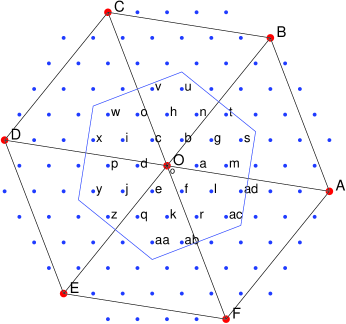
Figure 1: Hexagonal lattice $A_{2}$ and its sublattice with index $N=31$. Central lattice points are marked by small dots, and sublattice points by big dots.

Let $G$ and $G_{s}$ be generator matrices for $L$-dimensional central lattice $\Lambda$ and sublattice $\Lambda_{s}$. Then $\Lambda_{s}$ is geometrically similar to $\Lambda$ if and only if there exist an invertible $L\times L$ matrix $U$ with integer entries, a scalar $\beta$, and an orthogonal $L\times L$ matrix $A$ with determinant $1$ such that

$$G_{s}=UG=\beta GA,$$ (3)

The index for a geometrically similar lattice is $N=\frac{detG_{s}}{detG}=\beta^{L}$.

II-B Rate of MDLVQ

In MDLVQ, a source vector $x$ of joint pdf $g(x)$ is quantized to its nearest fine lattice $\lambda\in\Lambda$. The probability of quantizing $x$ to a lattice $\lambda$ is

$$P(\lambda)={\int_{V(\lambda)}}g(x)dx.$$ (4)

The entropy rate per dimension of the output of the central quantizer is [4]

$$\begin{split}R_{c}&=\frac{1}{L}\sum_{\lambda\in\Lambda}P(\lambda)\log P(\lambda)\\ &=-\frac{1}{L}\sum\limits_{\lambda\in\Lambda}{\int_{V(\lambda)}{g(x)dx}\log_{2}\int_{V(\lambda)}{g(x)dx}}\\ &\approx-\frac{1}{L}\sum\limits_{\lambda\in\Lambda}{\int_{V(\lambda)}{g(x)dx}\log_{2}g(\lambda)\nu}\\ &=h(p)-\frac{1}{L}\log_{2}\nu.,\end{split}$$ (5)

where $\nu$ is the volume of a Voronoi cell of $\Lambda$, and $h(p)$ is the differential entropy. The above assumes high resolution when $g(x)$ is approximately constant within a Voronoi cell $V(\lambda)$.

The volume of a Voronoi cell of the sublattice $\Lambda_{s}$ is ${\nu}_{s}=N\nu$. Denote by $Q(x)=\lambda$ the quantization mapping. Then, similarly to (5), the entropy rate per dimension of a side description (for balanced MDLVQ) is [4]

$$\begin{split}R_{s}&=\frac{1}{L}H(\alpha_{k}(Q(X)))\\ &\approx h(p)-\frac{1}{L}\log_{2}{\nu}_{s}\\ &=h(p)-\frac{1}{L}\log_{2}(N\nu).\end{split}$$ (6)

The total entropy rate per dimension for the balanced MDLVQ system is

$$R_{t}=KR_{s}.$$ (7)

II-C Distortion of MDLVQ

Assuming that the $K$ channels are independent and each has a failure probability $p$, we can write the expected distortion as

$$D=\sum_{k=0}^{K}{K\choose k}(1-p)^{k}p^{K-k}D_{k},$$

where $D_{k}$ is the expected distortion when receiving $k$ out of $K$ descriptions.

For the case of all descriptions received, the average distortion per dimension is given by

$$d_{c}=\sum\limits_{\lambda\in\Lambda}{\int_{V(\lambda)}{\left\|{x-\lambda}\right\|^{2}g(x)dx}}\approx G_{\Lambda}\nu^{\frac{2}{L}},$$ (8)

where $G_{\Lambda}$ is the dimensionless normalized second moment of lattice $\Lambda$ [14]. The approximation is under the standard high resolution assumption.

If only description $i$ is received, the expected side distortion is [4]

$$\begin{split}d_{i}&=\sum\limits_{\lambda\in\Lambda}{\int_{V(\lambda)}{\left\|{x-\lambda_{i}}\right\|^{2}g(x)dx}}\\ &=\sum\limits_{\lambda\in\Lambda}{\int_{V(\lambda)}\left(\left\|{x-\lambda}\right\|^{2}+\left\|{\lambda-\lambda_{i}}\right\|^{2}+2\langle x-\lambda,\lambda-\lambda_{i}\rangle\right)g(x)dx}\\ &\approx d_{c}+\sum\limits_{\lambda\in\Lambda}{\left\|{\lambda-\lambda_{i}}\right\|^{2}P(\lambda)},\ \ 1\leq i\leq K\end{split}$$ (9)

Hence the expected distortion when receiving only one description is

$$\begin{split}D_{1}&=\frac{1}{K}\sum_{i=1}^{K}d_{i}=d_{c}+\sum\limits_{\lambda\in\Lambda}\frac{1}{K}\sum\limits_{i=1}^{K}{\left\|{\lambda-\lambda_{i}}\right\|^{2}P(\lambda)}.\end{split}$$ (10)

Let $m_{K}$ be the centroid of all $K$ descriptions $\lambda_{1},\lambda_{2},\cdots,\lambda_{K}$, that it,

$$m_{K}\triangleq\frac{1}{K}\sum_{k=1}^{K}\lambda_{k}.$$ (11)

Then we have

$$\begin{split}\frac{1}{K}\sum\limits_{i=1}^{K}{\left\|{\lambda-\lambda_{i}}\right\|^{2}}&=\frac{1}{K}\sum\limits_{i=1}^{K}{\left\|{(\lambda-m_{K})-(\lambda_{i}-m_{K})}\right\|^{2}}\\ &=\left\|{\lambda-m_{K}}\right\|^{2}+\frac{1}{K}\sum\limits_{i=1}^{K}{\left\|{\lambda_{i}-m_{K}}\right\|^{2}}-\frac{2}{K}\left\langle{\lambda-m_{K},\sum\limits_{i=1}^{K}{(\lambda_{i}-m_{K})}}\right\rangle\\ &=\left\|{\lambda-m_{K}}\right\|^{2}+\frac{1}{K}\sum\limits_{i=1}^{K}{\left\|{\lambda_{i}-m_{K}}\right\|^{2}}.\end{split}$$ (12)

Substituting (12) into (10), we get

$$D_{1}=d_{c}+\sum\limits_{\lambda\in\Lambda}\left(\left\|{\lambda-m_{K}}\right\|^{2}+\frac{1}{K}\sum\limits_{i=1}^{K}\left\|{\lambda_{i}-m_{K}}\right\|^{2}\right)P(\lambda).$$ (13)

Now we consider the case of receiving $k$ descriptions, $1<k<K$. Let $\rm I$ be the set of all possible combinations of receiving $k$ out of $K$ descriptions. Let $\iota=(\iota_{1},\iota_{2},\cdots,\iota_{k})$ be an element of $\rm I$. Under high resolution assumption, we have [10]

$$\begin{split}D_{k}&=d_{c}+\left|\rm I\right|^{-1}\sum_{\lambda\in\Lambda}\sum_{\iota\in{\rm I}}\left\|\lambda-\frac{1}{k}{\sum_{j=1}^{k}\lambda_{\iota_{j}}}\right\|^{2}P(\lambda)\\ &=d_{c}+\sum\limits_{\lambda\in\Lambda}\left(\left\|{\lambda-m_{K}}\right\|^{2}+\frac{K-k}{(K-1)k}\frac{1}{K}\sum\limits_{i=1}^{K}{\left\|{\lambda_{i}-m_{K}}\right\|^{2}}\right)P(\lambda),\ \ 1<k<K.\end{split}$$ (14)

Substituting the expressions of $D_{k}$ into (II-C), we arrive at

$$D=(1-p^{K})d_{c}+\sum_{\lambda\in\Lambda}{\left({\zeta_{1}\left\|{\lambda-m_{K}}\right\|^{2}+\zeta_{2}\frac{1}{K}\sum_{i=1}^{K}{\left\|{\lambda_{i}-m_{K}}\right\|^{2}}}\right)}P(\lambda)+p^{K}E[\left\|X\right\|^{2}],$$ (15)

where

$$\begin{split}\zeta_{1}&=\sum_{k=1}^{K-1}{K\choose k}(1-p)^{k}p^{K-k}=1-p^{K}-(1-p)^{K}\\ \zeta_{2}&=\sum_{k=1}^{K-1}{K\choose k}(1-p)^{k}p^{K-k}\frac{K-k}{(K-1)k}.\end{split}$$ (16)

II-D Optimal MDLVQ Design

Given source and channel statistics and given total entropy rate $R_{t}$, optimal MDLVQ design involves (i) the choice of the central lattice $\Lambda$ and the sublattice $\Lambda_{s}$; (ii) the determination of optimal number of descriptions $K$ and of the optimal sublattice index value $N$; and (iii) the optimization of index assignment function $\alpha$ once (i) and (ii) are fixed. We defer the discussions of optimal values of $K$ and $N$ to Section IV, and first focus on the construction of optimal index assignment. It turns out that our new constructive approach will lead to improved analytical results of $K$ and $N$ in optimal MDLVQ design.

With fixed $p$, $K$, $\Lambda$, $\Lambda_{s}$, the optimal MDLVQ design problem (i.e., minimizing (15)) reduces to finding the optimal index assignment $\alpha$ that minimizes the average side distortion

$$d_{s}\triangleq\sum_{\lambda\in\Lambda}{\left(\frac{1}{K}\sum_{i=1}^{K}{\left\|\alpha_{i}(\lambda)-\mu(\alpha(\lambda))\right\|^{2}}+\zeta\left\|\lambda-\mu(\alpha(\lambda))\right\|^{2}\right)}P(\lambda),$$ (17)

where

$$\mu(\alpha(\lambda))=K^{-1}\sum_{i=1}^{K}\alpha_{i}(\lambda)$$

$$\begin{split}\zeta=\frac{\zeta_{1}}{\zeta_{2}}=\frac{\sum_{k=1}^{K-1}{K\choose k}(1-p)^{k}p^{K-k}}{\sum_{k=1}^{K-1}{K\choose k}(1-p)^{k}p^{K-k}\frac{K-k}{(K-1)k}}.\end{split}$$ (18)

When $K=2$, the objective function can be simplified to

$$\begin{split}d_{s}&=\sum_{\lambda\in\Lambda}{\left(\frac{1}{4}{\left\|{\lambda_{1}-\lambda_{2}}\right\|^{2}}+{\left\|{\lambda-\frac{\lambda_{1}+\lambda_{2}}{2}}\right\|^{2}}\right)}P(\lambda).\end{split}$$ (19)

III Index Assignment Algorithm

This section presents a new greedy index assignment algorithm for MDLVQ of $K\geq 2$ balanced descriptions and examines its optimality. The algorithm is very simple and it henges on an interesting new notion of $K$-fraction sublattice. We first define this $K$-fraction sublattice and reveal its useful properties for optimizing index assignment. Then we describe the greedy index assignment algorithm.

III-A $K$-fraction Sublattice

In the following study of optimal index assignment for $K$ balanced descriptions, the sublattice

$$\Lambda_{s/K}\triangleq\frac{1}{K}\Lambda_{s}=\{\tau\in\mathbb{R}^{L}:\tau=\frac{u}{K}G_{s},u\in\mathbb{Z}^{L}\}$$ (20)

plays an important role, and it will be referred as the $K$-fraction sublattice hereafter.

The $K$-fraction sublattice $\Lambda_{s/K}$ has the following interesting relations to $\Lambda$ and $\Lambda_{s}$.

Property 1

$\mu(\alpha(\lambda))=K^{-1}{\sum_{k=1}^{K}\alpha_{k}(\lambda)}$ is an onto (but not one-to-one) map: $\Lambda_{s}^{K}\to\Lambda_{s/K}$.

Proof:

1) $(\lambda_{1},\lambda_{2},\cdots,\lambda_{K})\in\Lambda_{s}^{K}\Rightarrow{\sum_{k=1}^{K}\lambda_{k}}\in\Lambda_{s}\to K^{-1}{\sum_{k=1}^{K}\lambda_{k}}\in\Lambda_{s/K}$; 2) $\forall\tau\in\Lambda_{s/K}$, let $\lambda_{1}=K\tau,\lambda_{2}=\cdots=\lambda_{K}=0$, then $\lambda_{1},\lambda_{2},\cdots,\lambda_{K}\in\Lambda_{s}$ and $\mu(\alpha(\lambda))=\tau$. ∎

This means that the centroid of any $K$-tuples in $\Lambda_{s}^{K}$ must be in $\Lambda_{s/K}$, and further $\Lambda_{s/K}$ consists only of these centroids.

If two $K$-fraction sublattice points $\tau_{1},\tau_{2}$ satisfy $\tau_{1}-\tau_{2}\in\Lambda_{s}$, then we say that $\tau_{1}$ and $\tau_{2}$ are in the same coset with respect to $\Lambda_{s}$. Any $K$-fraction sublattice point belong to one of the cosets.

Property 2

$\Lambda_{s/K}$ has, in the $L$-dimensional space, $K^{L}$ cosets with respect to $\Lambda_{s}$.

Proof:

Let $\tau_{1},\tau_{2}$ be two $K$-fraction sublattice points. $\tau_{1},\tau_{2}$ can be expressed by

$$\tau_{1}=\frac{u}{K}G_{s},\,\,\tau_{2}=\frac{v}{K}G_{s},$$

where $u=(u_{1},u_{2},\cdots,u_{L})\in\mathbb{Z}^{L},v=(v_{1},v_{2},\cdots,v_{L})\in\mathbb{Z}^{L}$. Two points $\tau_{1}$ and $\tau_{2}$ fall in the same coset with respect to $\Lambda_{s}$ if and only if $u_{i}\equiv v_{i}\bmod K$ for all $i=1,2,\cdots,L$. The claim follows since the reminder of division by $K$ takes on $K$ different values. ∎

The $K$-fraction sublattice $\Lambda_{s/K}$ partitions the space into Voronoi cells. Denote the Voronoi cell of a point $\tau\in\Lambda_{s/K}$ by

$$V_{s/K}(\tau)=\{x:\left\|{x-\tau}\right\|\leq\left\|{x-\tilde{\tau}}\right\|,\forall\tilde{\tau}\in\Lambda_{s/K}\}.$$

Property 3

$\Lambda_{s/K}$ is clean, if $\Lambda_{s}$ is clean.

Proof:

Assume for a contradiction that there was a point $\lambda\in\Lambda$ on the boundary of $V_{s/K}(\tau)$ for a $\tau\in\Lambda_{s/K}$. Scaling both $\lambda$ and $V_{s/K}(\tau)$ by $K$ places $K\lambda$ on the boundary of $KV_{s/K}(\tau)=\{Kx:\left\|{Kx-K\tau}\right\|\leq\left\|{Kx-K\tilde{\tau}}\right\|,\forall\tilde{\tau}\in\Lambda_{s/K}\}$. But $K\lambda$ is a point of $\Lambda$, and $KV_{s/K}(\tau)$ is nothing but the Voronoi cell $V_{s}$ of the sublattice point $K\tau\in\Lambda_{s}$, or the point $K\lambda\in\Lambda$ lies on the boundary of $V_{s}(K\tau)$, contradicting that $\Lambda_{s}$ is clean. ∎

Property 4

Both lattices $\Lambda_{s}$ and $\Lambda$ are symmetric about any point $\tau\in\Lambda_{s/2}$.

Proof:

$\forall\tau\in\Lambda_{s/2}$, we have $2\tau\in\Lambda_{s}$, so $2\tau-\lambda_{s}\in\Lambda_{s}$ holds for $\forall\lambda_{s}\in\Lambda_{s}$; similarly, $\forall\tau\in\Lambda_{s/2}$, we have $2\tau\in\Lambda$, so $2\tau-\lambda\in\Lambda$ holds for $\forall\lambda\in\Lambda$. ∎

III-B Greedy Index Assignment Algorithm

Our motive of constructing the $K$-fraction lattice $\Lambda_{s/K}$ is to relate $\Lambda_{s/K}$ to the central lattice $\Lambda$ in such a way that the two terms of $d_{s}$ in (17) can be minimized independently. This is brought into light by examining the partition of the space by Voronoi cells of $K$-fraction sublattice points. For simplicity, we assume the sublattice $\Lambda_{s}$ is clean (if not, the algorithm still works by employing a rule to break a tie on the boundary of a sublattice Voronoi cell). According to Property 3, no point $\lambda\in\Lambda$ is on the boundary of any Voronoi cell of $\Lambda_{s/K}$. Let

$$\ss(\tau)=\{(\lambda_{1},\lambda_{2},\cdots,\lambda_{K})\in\Lambda_{s}^{K}|\Sigma_{1\leq k\leq K}\lambda_{k}/K=\tau\}$$ (21)

be the set of all ordered $K$-tuples of sublattice points of centroid $\tau$, and $\tau\in\Lambda_{s/K}$ by Property 1.

In constructing an index assignment, we sort the members of $\ss(\tau)$ by $\sum_{k=1}^{K}\|\lambda_{k}-\tau\|^{2}$. From $\ss(\tau)$ we select the ordered $K$-tuples in increasing values of $\sum_{k=1}^{K}(\lambda_{k}-\tau)^{2}$ to label the central lattice points inside the $K$-fraction Voronoi cell $V_{s/K}(\tau)$, until all $N_{\tau}=|\Lambda\cap V_{s/K}(\tau)|$ of those central lattice points are labeled. It follows from (17) that any bijective mapping between the $n(\tau)$ central lattice points and the $N_{\tau}$ ordered $K$-tuples of sublattice points yields the same value of $d_{s}$. Such an index assignment clearly minimizes the second term of (17), which is the sum of the squared distances of all central lattice points in Voronoi cell $V_{s/K}(\tau)$ to the centroid $\tau=\mu(\alpha(\cdot))$. As $N\to\infty$, the proposed index assignment algorithm also minimizes the first term of (17) independently. This will be proven with some additional efforts in Section IV.

For the two description case, these $N_{\tau}$ ordered pairs are formed by the $N_{\tau}$ nearest sublattice points to $\tau$ in $\Lambda_{s}$ by Property 4. Note when $\tau\in\Lambda_{s}$, the ordered pair $(\tau,\tau)$ should be used to label $\tau$ itself.

According to Property 2, $\Lambda_{s/K}$ has $K^{L}$ cosets with respect to $\Lambda_{s}$ in the $L$-dimensional space, so there are $K^{L}$ classes of $V_{s/K}(\tau)$. We only need to label one representative out of each class, and cover the whole space by shifting. Thus it suffices to label a total of $N$ central lattice points.

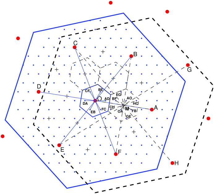
Figure 2: Optimal index assignments for $A_{2}$ lattice with $N=31$, $K=2$. Points of $\Lambda$, $\Lambda_{s}$ and $\Lambda_{s/2}$ are marked by $\cdot$, $\bullet$ and $+$, respectively.

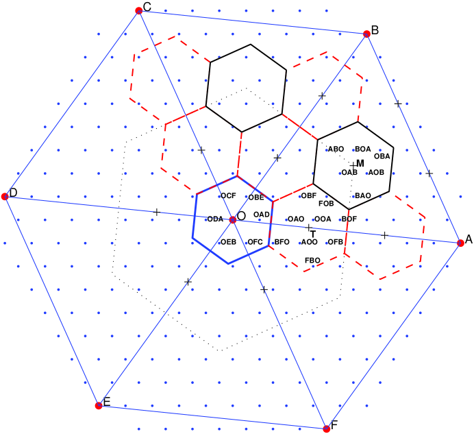
Figure 3: Optimal index assignments for $A_{2}$ lattice with $N=73$, $K=3$. Points of $\Lambda$, $\Lambda_{s}$ and $\Lambda_{s/3}$ are marked by $\cdot$, $\bullet$ and $+$, respectively.

To visualize the work of the proposed index assignment algorithm, let us examine two examples on an $A_{2}$ lattice (see Figs. 2 and 3). The $A_{2}$ lattice $\Lambda$ is generated by basis vectors represented by complex numbers: $1$ and $\omega=1/2+i{\sqrt{3}}/2$. By shifting invariance of $A_{2}$ lattice, we only need to label the $N$ central lattice points that belong to $K^{2}$ Voronoi cells of $\Lambda_{s/K}$. By angular symmetry of $A_{2}$ lattice, we can further reduce the number of points to be labeled.

The first example is a two-description case, with the sublattice $\Lambda_{s}$ given by basis vectors $5-\omega$, $\omega(5-\omega)$, which is geometrically similar to $\Lambda$, has index $N=31$ and is clean (refer to Fig. 2). There are two types of Voronoi cells of $\Lambda_{s/2}$, as shown by the solid and dashed boundaries in Fig. 2. The solid cell is centered at a central lattice point and contains $7$ central lattice points. The dashed cell is centered at the midpoint of the line segment $OA$, and contains $8$ central lattice points. To label the $7$ central lattice points in $V_{s/2}(O)$, we use the $7$ nearest sublattice points to $O$: $(O,A,B,C,D,E,F)$. They form $6$ ordered pairs with the midpoint $O$ : $((A,D),(D,A),(B,E),(E,B),(C,F),(F,C)$, and an unordered pair $(O,O)$ since $O$ is itself a sublattice point. To label the $8$ central lattice points in $V_{s/2}(M)$, we use the $8$ nearest sublattice points to $M$: $(O,A,B,F,C,H,E,G)$. They form $8$ ordered pairs with midpoint $M$: $(O,A)$, $(A,O)$, $(B,F)$, $(F,B)$, $(C,H)$, $(H,C)$, $(E,G)$, $(G,E)$. The labeling of the $7$ central lattice points in $V_{s/2}(O)$ and the labeling of the $8$ central lattice points in $V_{s/2}(M)$ are illustrated in Fig. 2.

Fig. 3 illustrates the result of the proposed algorithm in the case of three descriptions. The depicted index assignment for three balanced descriptions is computed for the sublattice of index $N=73$ and basis vectors: $8-\omega$, $\omega(8-\omega)$.

The presented MDLVQ index assignment algorithm is fast with an $O(N)$ time complexity. The simplicity and low complexity of the algorithm are due to the greedy optimization approach adopted.

The tantalizing question is, of course, can the greedy algorithm be optimal? A quick test on the above two examples may be helpful. Let the distance between a nearest pair of central lattice points in $\Lambda$ be one. For the first example the result of [4] (the best so far) is $d_{s}=561/31=18.0968$, while the greedy algorithm does better, producing $d_{s}=528/31=17.0323$. Indeed, in both examples, one can verify that the expected distortion is minimized as the two terms of $d_{s}$ in (17) are minimized independently.

IV Asymptotically Optimal Design of MDLVQ

In this section we first prove that the greedy index assignment is optimal for any $K$, $p$, $\Lambda$ and $\Lambda_{s}$ as $N\rightarrow\infty$. In constructing the proof we derive a close form asymptotical expression of the expected distortion of optimal MDLVQ for general $K\geq 2$. It allows us to determine the optimal volume of a central lattice Voronoi cell $\nu$, the optimal sublattice index $N$, and the optimal number of descriptions $K$, given the total entropy rate of all side descriptions $R_{t}$ and the loss probability $p$. These results, in addition to optimal index assignment $\alpha$, complete the design of optimal MDLVQ, and they present an improvement over previous work of [10].

IV-A Asymptotical Optimality of the Proposed Index Assignment

Since the second term of $d_{s}$ is minimized by the Voronoi partition defined by the $K$-fraction lattice, the optimality of the proposed index assignment based on the $K$-fraction lattice follows if it also minimizes the first term of $d_{s}$. This is indeed the case when $N\to\infty$. To compute the first term of $d_{s}$, let

$$\varsigma_{k}\triangleq\sum_{i=1}^{k}\lambda_{i},k=1,2,\cdots,K,$$

Then

$$\begin{split}\sum_{k=1}^{K}{\left\|{\lambda_{k}-\tau}\right\|^{2}}&=\sum_{k=1}^{K}\left\|\lambda_{k}-\frac{1}{K}\varsigma_{K}\right\|^{2}\\ &=\left(\sum_{k=1}^{K-1}\left\|\lambda_{k}-\frac{1}{K}\varsigma_{K}\right\|^{2}\right)+\left\|\lambda_{K}-\frac{1}{K}\varsigma_{K}\right\|^{2}\\ &=\left(\sum_{k=1}^{K-1}\left\|\left(\lambda_{k}-\frac{1}{K-1}\varsigma_{K-1}\right)+\frac{1}{K-1}\left(\varsigma_{K-1}-\frac{K-1}{K}\varsigma_{K}\right)\right\|^{2}\right)+\left\|\varsigma_{K-1}-\frac{K-1}{K}\varsigma_{K}\right\|^{2}\\ &\overset{(a)}{=}\left(\sum_{k=1}^{K-1}{\left\|{\lambda_{k}-\frac{1}{K-1}\varsigma_{K-1}}\right\|^{2}}\right)+\frac{K}{K-1}{\left\|{\varsigma_{K-1}-\frac{K-1}{K}\varsigma_{K}}\right\|^{2}}\\ &\overset{(b)}{=}\sum_{k=1}^{K-1}\frac{k+1}{k}{\left\|\varsigma_{k}-\frac{k}{k+1}\varsigma_{k+1}\right\|^{2}}.\end{split}$$ (22)

Equality $(a)$ holds because the inner product $\left<\sum_{k=1}^{K-1}\left({\lambda_{k}-\frac{1}{K-1}\varsigma_{K-1}}\right),\frac{1}{K-1}\left(\varsigma_{K-1}-\frac{K-1}{K}\varsigma_{K}\right)\right>$ is zero. After using the same deduction $K-1$ times, we arrive at equality $(b)$.

Note the one-to-one correspondence between $(\lambda_{1},\lambda_{2},\cdots,\lambda_{K})$ and $(\varsigma_{1},\varsigma_{2},\cdots,\varsigma_{K})$. Also recall that the proposed index assignment uses the $N_{\tau}$ (the number of central lattice points in $K$-fraction Voronoi cell $V_{s/K}(\tau)$) smallest $K$-tuples in $\ss(\tau)$ according to the value of $\sum_{k=1}^{K}\|\lambda_{k}-\tau\|^{2}$. Finding the $N_{\tau}$ smallest values of $\sum_{k=1}^{K}\|\lambda_{k}-\tau\|^{2}$ in $\ss(\tau)$ is equivalent to finding the $N_{\tau}$ smallest values of $\sum_{k=1}^{K-1}\frac{k+1}{k}{\left\|\varsigma_{k}-\frac{k}{k+1}\varsigma_{k+1}\right\|^{2}}$ among the $(K-1)$-tuples $(\varsigma_{1},\varsigma_{2},\cdots,\varsigma_{K-1})$ with $\varsigma_{K}=\sum_{k=1}^{K}\lambda_{k}$.

Theorem 1

The proposed greedy index assignment algorithm is optimal as $N\to\infty$ for any given $\Lambda$, $\Lambda_{s}$, $K$, and $p$.

Proof:

The $i^{th}$ nearest sublattice point to $\frac{k}{k+1}\varsigma_{k+1}$ is approximately on the boundary of an $L$-dimensional sphere with volume $iN\nu$. Given $\varsigma_{k+1}$, the $i^{th}$ smallest value of $\|\varsigma_{k}-\frac{k}{k+1}\varsigma_{k+1}\|^{2}$ is approximately $(iN\nu/B_{L})^{\frac{2}{L}}/L=G_{L}(1+\frac{2}{L})(iN\nu)^{\frac{2}{L}}$, where $B_{L}=G_{L}^{-\frac{L}{2}}(L+2)^{-\frac{L}{2}}$ is the volume of an $L$-dimensional sphere of unit radius [4], and $G_{L}$ is the dimensionless normalized second moment of an $L$-dimensional sphere.

Let $f^{(n)}(\tau)$ be the $n^{th}$ smallest value of $\sum_{k=1}^{K}{\left\|{\lambda_{k}-\tau}\right\|^{2}}$ in $\ss(\tau)$ that is realized at $(\varsigma_{1}^{(n)},\varsigma_{2}^{(n)},\cdots,\varsigma_{K-1}^{(n)})$. Then

$$\begin{split}f^{(n)}(\tau)&=\sum_{k=1}^{K-1}\frac{k+1}{k}{\left\|\varsigma_{k}^{(n)}-\frac{k}{k+1}\varsigma_{k+1}^{(n)}\right\|^{2}}\\ &\approx G_{L}\left(1+\frac{2}{L}\right)(N\nu)^{\frac{2}{L}}\sum_{k=1}^{K-1}\frac{k+1}{k}(i_{k}^{(n)})^{\frac{2}{L}},\end{split}$$ (23)

in which $(i_{1}^{(n)},i_{2}^{(n)},\cdots,i_{K-1}^{(n)})\in\mathbb{Z}^{K-1}$ is where the sum $\sum_{k=1}^{K-1}\frac{k+1}{k}(i_{k})^{\frac{2}{L}}$ takes on its $n^{th}$ smallest value over all $(K-1)$-tuples of positive integers.

When $N\to\infty$, the proposed index assignment algorithm takes the $N_{\tau}\approx N/K^{L}$ smallest terms of $\sum_{k=1}^{K}{\left\|{\lambda_{k}-\tau}\right\|^{2}}$ in $\ss(\tau)$ for every $\tau$. But (23) states that the $n^{th}$ smallest value of $\sum_{k=1}^{K}{\left\|{\lambda_{k}-\tau}\right\|^{2}}$ is independent of $\tau$. Therefore, the first term of $d_{s}$ is minimized, establishing the optimality of the resulting index assignment. ∎

Remark IV.1: The $O(N)$ MDLVQ index assignment algorithm based on the $K$-fraction lattice is so far the only one proven to be asymptotically optimal, except for the prohibitively expensive linear assignment algorithm. In the next section, we will strengthen the above proof in a constructive perspective, and establish the optimality of the algorithm for finite $N$ when $K=2$.

IV-B Optimal Design Parameters $\nu$, $N$ and $K$

Now our attention turns to the determination of the optimal $\nu$ (the volume of a Voronoi cell of $\Lambda$), $N$ (the sublattice index) and $K$ (the number of descriptions) that achieve minimum expected distortion, given the total entropy rate of all side descriptions $R_{t}$ and loss probability $p$.

Using (23), we have

$$\begin{split}\sum_{\lambda\in\Lambda}\sum_{k=1}^{K}\left\|\lambda_{k}-\mu(\alpha(\lambda))\right\|^{2}P(\lambda)&=\sum_{\tau\in\Lambda_{s/K}}\sum_{\lambda\in V_{s/K}(\tau)}\sum_{k=1}^{K}\left\|{\lambda_{k}-\mu(\alpha(\lambda))}\right\|^{2}P(\lambda)\\ &\approx\frac{1}{N_{\tau}}\sum_{n=1}^{N_{\tau}}\sum_{k=1}^{K-1}\frac{k+1}{k}{\left\|\varsigma_{k}^{(n)}-\frac{k}{k+1}\varsigma_{k+1}^{(n)}\right\|^{2}}\\ &\approx G_{L}(1+\frac{2}{L})\left(N\nu\right)^{\frac{2}{L}}\frac{1}{N_{\tau}}\sum_{n=1}^{N_{\tau}}\sum_{k=1}^{K-1}\frac{k+1}{k}(i_{k}^{(n)})^{\frac{2}{L}}\end{split}$$ (24)

Consider the region defined as

$$\Omega\triangleq\left\{\sum_{k=1}^{K-1}\frac{k+1}{k}x_{k}^{\frac{2}{L}}\leq C\left|x_{1},x_{2},\cdots,x_{K-1}\geq 0,\\ x_{1},x_{2}\cdots,x_{K-1}\in\mathbb{R}\right.\right\}.$$ (25)

Choose $C$ appropriately so that the volume of $\Omega$ is $V(\Omega)=N_{\tau}$. As $N_{\tau}\rightarrow\infty$, $\Omega$ contains approximately $N_{\tau}$ optimal integer vectors $(i_{1},i_{2},\cdots,i_{K-1})$. These $N_{\tau}$ points are uniformly distributed in $\Omega$, with density one point per unit volume. Because the ratio between the volume occupied by each point and the total volume is $1/N_{\tau}$, which approaches zero when $N_{\tau}\rightarrow\infty$, we can replace the summation by integral and get

$$\begin{split}\frac{1}{N_{\tau}}\sum_{n=1}^{N_{\tau}}\sum_{k=1}^{K-1}\frac{k+1}{k}(i_{k}^{(n)})^{\frac{2}{L}}&\approx\frac{\int_{x\in\Omega}\sum_{k=1}^{K-1}\frac{k+1}{k}x_{k}^{\frac{2}{L}}\,dx}{\int_{x\in\Omega}\,dx}\\ &=\frac{\int_{y\in\Omega_{0}}\sum_{k=1}^{K-1}y_{k}^{\frac{2}{L}}\,dy}{\int_{y\in\Omega_{0}}\,dy},\end{split}$$ (26)

where $y_{k}=(\frac{k+1}{k})^{\frac{L}{2}}x_{k},k=1,2,\cdots,K-1$, and $\Omega_{0}$ is defined as

$$\Omega_{0}\triangleq\left\{\sum_{k=1}^{K-1}y_{k}^{\frac{2}{L}}\leq C\left|y_{1},y_{2},\cdots,y_{K-1}\geq 0,\\ y_{1},y_{2}\cdots,y_{K-1}\in\mathbb{R}\right.\right\}.$$ (27)

Substituting (26) into (24), we have

$$\sum_{\lambda\in\Lambda}\sum_{k=1}^{K}\left\|{\lambda_{k}-\mu(\alpha(\lambda))}\right\|^{2}P(\lambda)\approx G_{L}(1+\frac{2}{L})\left(N\nu\right)^{\frac{2}{L}}\frac{\int_{y\in\Omega_{0}}\sum_{k=1}^{K-1}y_{k}^{\frac{2}{L}}\,dy}{\int_{y\in\Omega_{0}}\,dy}.$$ (28)

Let $V(\Omega_{0})$ be the volume of region $\Omega_{0}$, i.e.,

$$\begin{split}V(\Omega_{0})&=\int_{y\in\Omega_{0}}\,dy_{1}\,dy_{2}\cdots\,dy_{K-1}\\ &=K^{\frac{L}{2}}\int_{x\in\Omega}\,dx_{1}\,dx_{2}\cdots\,dx_{K-1}\\ &=K^{\frac{L}{2}}N_{\tau}\\ &=K^{-\frac{L}{2}}N,\end{split}$$ (29)

and define the dimensionless normalized $\frac{2}{L}$th moment of $\Omega_{0}$:

$$G_{\Omega_{0}}\triangleq\frac{1}{K-1}\frac{\int_{y\in\Omega_{0}}\sum_{k=1}^{K-1}y_{k}^{\frac{2}{L}}\,dy}{V(\Omega_{0})^{1+\frac{2}{L(K-1)}}}.$$ (30)

Note that scaling $\Omega_{0}$ does not change $G_{\Omega_{0}}$. For the special case $L=1$, the region $\Omega_{0}$ is a $(K-1)$-dimensional sphere in the first octant, so the normalized second moment $G_{\Omega_{0}}=4G_{K-1}$. For the special case $K=2$, $G_{\Omega_{0}}=L/(L+2)$ is the normalized $\frac{2}{L}$th moment of a line $[0,C]$. Generally, using Dirichilet’s Integral [16], we get

$$G_{\Omega_{0}}=\frac{1}{n+\frac{2}{L}}\frac{\Gamma(\frac{nL}{2}+1)^{\frac{2}{nL}}}{\Gamma(\frac{L}{2}+1)^{\frac{2}{L}}}.$$ (31)

Hence,

$$\frac{\int_{y\in\Omega_{0}}\sum_{k=1}^{K-1}y_{k}^{\frac{2}{L}}\,dy}{\int_{y\in\Omega_{0}}\,dy}=G_{\Omega_{0}}(K-1)V(\Omega_{0})^{\frac{2}{L(K-1)}}=G_{\Omega_{0}}(K-1)K^{\frac{-1}{K-1}}N^{\frac{2}{L(K-1)}}.$$ (32)

Substituting (32) into (28), we have

$$\begin{split}\frac{1}{K}\sum_{\lambda\in\Lambda}\sum_{k=1}^{K}\left\|{\lambda_{k}-\mu(\alpha(\lambda))}\right\|^{2}P(\lambda)&\approx G_{L}G_{\Omega_{0}}(1+\frac{2}{L})(K-1)K^{\frac{-K}{K-1}}N^{\frac{2K}{L(K-1)}}\nu^{\frac{2}{L}}\\ &\approx G_{L}\Phi_{K-1,L}(K-1)K^{\frac{-K}{K-1}}N^{\frac{2K}{L(K-1)}}\nu^{\frac{2}{L}},\end{split}$$ (33)

where

$$\Phi_{n,L}=\frac{1+\frac{2}{L}}{n+\frac{2}{L}}\frac{\Gamma(\frac{nL}{2}+1)^{\frac{2}{nL}}}{\Gamma(\frac{L}{2}+1)^{\frac{2}{L}}}.$$

Note $\Phi_{n,1}=12G_{n}$ and $\Phi_{1,L}=1$.

When $N\to\infty$, $N_{\tau}\approx N/K^{L}$ independently of the cell center $\tau$. The $N_{\tau}$ central lattice points are uniformly distributed in $V_{s/K}(\tau)$ whose volume is approximately $N_{\tau}\nu$. Hence the second term of $d_{s}$ can be evaluated as

$$\begin{split}\zeta\sum_{\lambda\in\Lambda}\left\|{\lambda-\mu(\alpha(\lambda))}\right\|^{2}P(\lambda)&\approx\zeta G_{\Lambda}(N_{\tau}\nu)^{\frac{2}{L}}\\ &=\zeta G_{\Lambda}K^{-2}(N\nu)^{\frac{2}{L}}.\end{split}$$ (34)

Comparing (34) with (33), the first term of $d_{s}$ dominates the second term when $N\rightarrow\infty$, thus

$$d_{s}\approx G_{L}\Phi_{K-1,L}(K-1)K^{\frac{-K}{K-1}}N^{\frac{2K}{L(K-1)}}\nu^{\frac{2}{L}}.$$ (35)

Substituting (35) and (8) into (15), we finally express the expected distortion of optimal MDLVQ in a closed form:

$$D\approx(1-p^{K})G_{\Lambda}{\nu}^{\frac{2}{L}}+\zeta_{2}G_{L}\Phi_{K-1,L}(K-1)K^{\frac{-K}{K-1}}N^{\frac{2K}{L(K-1)}}\nu^{\frac{2}{L}}+p^{K}E[\|X\|^{2}].$$ (36)

Using a different index assignment algorithm Østergaard et al. derived a similar expression for the expected MDLVQ distortion (equation (35) in [10]):

$$D^{*}\approx(1-p^{K})G_{\Lambda}{\nu}^{\frac{2}{L}}+\hat{K}G_{L}\psi_{L}^{2}N^{\frac{2K}{L(K-1)}}\nu^{\frac{2}{L}}+p^{K}E[\|X\|^{2}],$$ (37)

where

$$\hat{K}=\sum_{k=1}^{K-1}{K\choose k}(1-p)^{k}p^{K-k}\frac{K-k}{2kK}$$ (38)

and $\psi_{L}$ is a quantity that is given analytically only for $K=2$ and for $K=3$ with odd $L$ and is determined empirically for other cases.

To compare $D$ and $D^{*}$, we rewrite (36) as

$$D\approx(1-p^{K})G_{\Lambda}{\nu}^{\frac{2}{L}}+\hat{K}G_{L}\hat{\psi}_{L}^{2}N^{\frac{2K}{L(K-1)}}\nu^{\frac{2}{L}}+p^{K}E[\|X\|^{2}],$$ (39)

where

$$\hat{\psi}_{L}=\sqrt{2K^{\frac{-1}{K-1}}\Phi_{K-1,L}}.$$ (40)

The two expressions are the same when $K=2$ for which $\hat{\psi}_{L}=\psi_{L}=1$, but they differ for $K>2$. Table I lists the values of $\psi_{L}$ and $\hat{\psi}_{L}$ for $K=3$, and it shows that $\hat{\psi}_{\infty}=\psi_{\infty}=(\frac{4}{3})^{\frac{1}{4}}$, and $\hat{\psi}_{L}<\psi_{L}$ for other values of $L$. This implies $D<D^{*}$, or that our index assignment makes the asymptotical expression of $D$ tighter.

$L$	$\psi_{L}$	$\hat{\psi}_{L}...$
$1$	$1.1547...$	$0.9549...$
$2$	$1.1481...$	$0.9428...$
$3$	$1.1346...$	$0.9394...$
$5$	$1.1241...$	$0.9400...$
$7$	$1.1173...$	$0.9431...$
$9$	$1.1125...$	$0.9466...$
$11$	$1.1089...$	$0.9498...$
$13$	$1.1060...$	$0.9527...$
$15$	$1.1036...$	$0.9552...$
$17$	$1.1017...$	$0.9575...$
$19$	$1.1000...$	$0.9596...$
$21$	$1.0986...$	$0.9614...$
$51$	$1.0884...$	$0.9763...$
$71$	$1.0856...$	$0.9807...$
$101$	$1.0832...$	$0.9848...$
$\infty$	$1.0746...$	$1.0746...$

TABLE I: Values of $\psi_{L}$ and $\hat{\psi}_{L}$ in $L$ for $K=3$. Values of $\psi_{L}$ are reproduced from Table $1$ in [10].

Now we proceed to derive the optimal value of $N$, which governs the optimal trade-off between the central and side distortions for given $p$ and $K$. For the total target entropy rate $R_{t}=KR$, we rewrite (5) to get

$$N\nu=2^{L(h(p)-R_{t}/K)}.$$ (41)

For simplicity, define

$$\eta\triangleq 2^{L(h(p)-R_{t}/K)},$$ (42)

and we have

$$D=(1-p^{K})G_{\Lambda}{\nu}^{\frac{2}{L}}+\zeta_{2}G_{L}\Phi_{K-1,L}(K-1)K^{\frac{-K}{K-1}}{\eta}^{\frac{2K}{L(K-1)}}\nu^{\frac{-2}{L(K-1)}}+p^{K}E[\|X\|^{2}].$$ (43)

Differentiating $D$ with respect to $\nu$ yields the optimal $\nu$ value:

$$\nu_{opt}=\eta\left(\frac{\zeta_{2}}{1-p^{K}}\frac{G_{L}}{G_{\Lambda}}\frac{\Phi_{K-1,L}}{K^{\frac{K}{K-1}}}\right)^{\frac{L(K-1)}{2K}}.$$

Substituting $\nu_{opt}$ to (41), we get optimal $N$:

$$N_{opt}=\left(\frac{1-p^{K}}{\zeta_{2}}\frac{G_{\Lambda}}{G_{L}}\frac{K^{\frac{K}{K-1}}}{\Phi_{K-1,L}}\right)^{\frac{L(K-1)}{2K}}.$$ (44)

If $K=2$, the expression of $N_{opt}$ can be simplified as

$$N_{opt}=\left(\frac{2(1+p)}{p}\frac{G_{\Lambda}}{G_{L}}\right)^{\frac{L}{4}}.$$ (45)

Remark IV.2: $N_{opt}$ is independent of the total target entropy rate $R_{t}$ and source entropy rate $h(p)$. It only depends on the loss probability $p$ and on the number of descriptions $K$. Substituting $\nu_{opt}$ into (43), the average distortion can be expressed as a function of $K$. Then optimal $K$ can be solved numerically.

Remark IV.3: When $K=2$, (35) can be simplified to

$$d_{s}\approx\frac{1}{4}G_{L}(N^{2}\nu)^{\frac{2}{L}}.$$ (46)

For any $a\in(0,1)$, let $N=2^{L(aR+1)}$, then $\nu=2^{L(h(p)-(a+1)R-1)}$. Since $R\rightarrow\infty$ implies $N\rightarrow\infty$, substituting the expressions of $N$ and $\nu$ into (8) and (46), we get

$$\mathop{\lim}\limits_{R\to\infty}d_{c}2^{2R(1+a)}=\frac{1}{4}G_{\Lambda}2^{2h(p)}$$

$$\mathop{\lim}\limits_{R\to\infty}d_{k}2^{2R(1-a)}=G_{L}2^{2h(p)},\ \ k=1,2$$

Therefore, the proposed MDLVQ algorithm asymptotically achieves the second-moment gain of a lattice for the central distortion, and the second-moment gain of a sphere for the side distortion, which is the same as the expression in [4]. In other words, our algorithm realizes the MDC performance bound for two balanced descriptions.

V Non-asymptotical Optimality for $K=2$

In this section we sharpen the results of the previous section, by proving non-asymptotical (i.e., with respect to a finite $N$) optimality and deriving an exact distortion formula of our MDLVQ design algorithm for $K=2$ balanced descriptions, under mild conditions. The following analysis is constructive and hence more useful than an asymptotical counterpart because the value of $N$ is not very large in practice [7].

V-A A Non-asymptotical Proof

Our non-asymptotical proof is built upon the following definitions and lemmas.

Definition 1

A sublattice $\Lambda_{s}$ is said to be centric, if the sublattice Voronoi cell $V_{s}(\lambda)$ centered at $\lambda\in\Lambda_{s}$ contains the $N$ nearest central lattice points to $\lambda$.

Figs. 2 and 3 show two examples of centric sublattices.

To prove the optimality of the greedy algorithm, we need some additional properties.

Lemma 1

Assume the sublattice $\Lambda_{s}$ is centric. If $\lambda\in V_{s/2}(\tau)$ and $\tilde{\lambda}\not\in V_{s/2}(\tilde{\tau})$, where $\lambda,\tilde{\lambda}\in\Lambda$ and $\tau,\tilde{\tau}\in\Lambda_{s/2}$, then $\|{\lambda-\tau}\|\leq\|{\tilde{\lambda}-\tilde{\tau}}\|$.

Proof:

Scaling both $\lambda$ and $V_{s/2}(\tau)$ by $2$ places the lattice point $2\lambda$ in $V_{s}(2\tau)$; scaling both $\tilde{\lambda}$ and $V_{s/2}(\tilde{\tau})$ by $2$ places the lattice point $2\tilde{\lambda}\not\in V_{s}(2\tilde{\tau})$. Since a sublattice Voronoi cell contains the nearest central lattice points, $\|{2\lambda-2\tau}\|\leq\|{2\tilde{\lambda}-2\tilde{\tau}}\|$, and hence $\|{\lambda-\tau}\|\leq\|{\tilde{\lambda}-\tilde{\tau}}\|$. ∎

Definition 2

A sublattice $\Lambda_{s}$ is said to be $S$-similar to $\Lambda$, if $\Lambda_{s}$ can be generated by scaling and rotating $\Lambda$ around any point $\tau\in\Lambda_{s/2}$ and $\Lambda_{s}\subset\Lambda$.

Note that the $S$-similarity requires that the center of symmetry be a point in $\Lambda_{s/2}$.

In what follows we assume that sublattice $\Lambda_{s}$ is $S$-similar to $\Lambda$. Also, we denote by $V_{\tau}$ the region created by scaling and rotating $V_{s/2}(\tau)$ around $\tau$.

Lemma 2

If $\lambda_{s}\in V_{\tau}$ and $\tilde{\lambda}_{s}\not\in V_{\tilde{\tau}}$, where $\lambda_{s},\tilde{\lambda}_{s}\in\Lambda_{s}$ and $\tau,\tilde{\tau}\in\Lambda_{s/2}$, then $\|{\lambda_{s}-\tau}\|\leq\|{\tilde{\lambda}_{s}-\tilde{\tau}}\|$.

Proof:

This lemma follows from Lemma 1 and the definition of $S$-Similar. ∎

Lemma 3

$\forall\tau\in\Lambda_{s/2}$, the sublattice points in $V_{\tau}$ form $|\Lambda\cap V_{s/2}(\tau)|$ nearest ordered $2$-tuples with their midpoints being $\tau$.

Proof:

Letting $\tilde{\tau}=\tau$ in Lemma 2, we see that $V_{\tau}$ contains the $|\Lambda_{s}\cap V_{\tau}|=|\Lambda\cap V_{s/2}(\tau)|$ nearest sublattice points to $\tau$. And these sublattice points are symmetric about $\tau$ according to Property 4. Thus this lemma holds. ∎

Theorem 2

The proposed index assignment algorithm is optimal for $K=2$ and any $N$, if the sublattice is centric and $S$-Similar to the associated central lattice.

Proof:

By Property 1, for any $\lambda_{1},\lambda_{2}\in\Lambda_{s}$, $(\lambda_{1}+\lambda_{2})/2\in\Lambda_{s/2}$. Now referring to (19), the proposed algorithm minimizes the second term $\sum_{\lambda\in\Lambda}{\|{\lambda-(\lambda_{1}+\lambda_{2})/2}\|^{2}P(\lambda)}$ of $d_{s}$, since it labels any central lattice point $\lambda\in V_{s/2}(\tau)$ by $(\lambda_{1},\lambda_{2})\in\Lambda_{s}^{2}$, and $(\lambda_{1}+\lambda_{2})/2=\tau$.

The algorithm also independently minimizes the first term $\sum_{\lambda\in\Lambda}\frac{1}{4}{\|{\lambda_{1}-\lambda_{2}}\|^{2}P(\lambda)}$ of $d_{s}$. Assume that $\sum_{\lambda\in\Lambda}{\|{\lambda_{1}-\lambda_{2}}\|^{2}P(\lambda)}$ was not minimized. Then there exists an ordered $2$-tuple $(\tilde{\lambda}_{1},\tilde{\lambda}_{2})\in\Lambda_{s}^{2}$ which is not used in the index assignment, and $\|{\tilde{\lambda}_{1}-\tilde{\lambda}_{2}}\|<\|{\lambda_{1}-\lambda_{2}}\|$, where $(\lambda_{1},\lambda_{2})\in\Lambda_{s}^{2}$ is used in the index assignment. Let $\tau=(\lambda_{1}+\lambda_{2})/2,\tilde{\tau}=(\tilde{\lambda}_{1}+\tilde{\lambda}_{2})/2$. Since $(\lambda_{1},\lambda_{2})$ is used to label a central lattice point in $V_{s/2}(\tau)$, $\lambda_{1},\lambda_{2}\in V_{\tau}$ by Lemma 3. However, $\tilde{\lambda}_{1},\tilde{\lambda}_{2}\not\in V_{\tilde{\tau}}$, otherwise $(\tilde{\lambda}_{1},\tilde{\lambda}_{2})$ would be used in the index assignment by Lemma 3. So we have $\|{\lambda_{1}-\tau}\|\leq\|{\tilde{\lambda}_{1}-\tilde{\tau}}\|$ by Lemma 2, hence $\|{\lambda_{1}-\lambda_{2}}\|\leq\|{\tilde{\lambda}_{1}-\tilde{\lambda}_{2}}\|$, contradicting $\|{\tilde{\lambda}_{1}-\tilde{\lambda}_{2}}\|<\|{\lambda_{1}-\lambda_{2}}\|$. ∎

Remark V.1: A sublattice Voronoi cell being centric is not a necessary condition for the optimality of the greedy algorithm. For instance, for the $A_{2}$ lattice generated by basis vectors $1$ and $\omega=1/2+i{\sqrt{3}}/2$ and the sublattice of index $N=91$ that is generated by basis vectors $9-\omega$, $\omega(9-\omega)$, a sublattice Voronoi cell does not contain the $N$ nearest central lattices, but the greedy algorithm is still optimal as the two terms of $d_{s}$ are still independently minimized. This is shown in Figure 4.

Figure 4: The greedy algorithm is optimal for $N=91$, although the sublattice is not centric. The $19$ central lattice points in $V_{s/2}(O)$ are labeled by the $19$ nearest ordered $2$-tuples with centroid $O$. The $24$ central lattice points in $V_{s/2}(M)$ are labeled by the $24$ nearest ordered $2$-tuples with centroid $M$. Let the edge length of $2$-tuple $(O,A)$ be one: $||O-A||\triangleq 1$. The $19th$ $(20th)$ nearest ordered $2$-tuple with centroid $O$ has edge length $4$ $(2\sqrt{7})$. The $24th$ $(25th)$ nearest ordered $2$-tuple with centroid $M$ has edge length $5$ $(3\sqrt{3})$. Because $4<3\sqrt{3}$ and $5<2\sqrt{7}$, the first term of $d_{s}$ is minimized. The second term of $d_{s}$ is minimized because the greedy algorithm partition the space by the Voronoi cells of the $K$-fraction sublattice.

Remark V.2: It is easy to choose a centric sublattice for relatively small $N$ and in high dimensional lattices. For instance, the sublattices of $A_{2}$ lattice shown in Fig. 2, Fig. 3 are centric. And any sublattice of $Z$ lattice is centric.

V-B Exact Distortion Formula for $K=2$

We have derived an asymptotical expected distortion formula (36) of the proposed MDLVQ design, which improved a similar result in [10]. But so far no exact non-asymptotical expression of the expected MDLVQ distortion is known even for balanced two descriptions. This subsection presents a progress on this account.

Lemma 4

If the sublattice is clean and $S$-similar, then the second term of $d_{s}$ for the proposed optimal MDLVQ design for $K=2$ is

$$\sum_{\lambda\in\Lambda}{{\left\|{\lambda-m_{1,2}}\right\|^{2}P(\lambda)}}=\frac{1}{4L}\frac{\sum_{i=1}^{N}a_{i}}{N},$$ (47)

where $a_{i}$ is the squared distance of the $i^{th}$ nearest central lattice point in $V_{s}(0)$ to the origin.

Proof:

$\Lambda_{s/2}$ has $2^{L}$ cosets with respective to $\Lambda_{s}$ in the $L$-dimensional space. Let $\tau_{1},\tau_{2},\cdots,\tau_{2^{L}}$ be representatives of each coset. For example, when $L=2$, $\tau_{1}=(0,0)G_{s},\tau_{2}=(0,\frac{1}{2})G_{s},\tau_{3}=(\frac{1}{2},0)G_{s},\tau_{4}=(\frac{1}{2},\frac{1}{2})G_{s}$. Denote by $V_{\lambda}(\tau)\triangleq V_{s/2}(\tau)\bigcap\Lambda$ the set of central lattice points in the Voronoi cell of a $2$-fraction sublattice point $\tau$. We first prove that

$$2\left(V_{\lambda}(\tau_{i})-\tau_{i}\right)\mathop{\cap}_{i\neq j}2\left(V_{\lambda}(\tau_{j})-\tau_{j}\right)=\varnothing.$$ (48)

$$\mathop{\cup}_{i=1}^{2^{L}}2\left(V_{\lambda}(\tau_{i})-\tau_{i}\right)=V_{s}(0)\cap\Lambda.$$ (49)

Here for convenience, we denote by $2V$ the set of lattice points that is generated by scaling the lattice points in Voronoi cell $V$ by $2$.

Assume that (48) does not hold. Then there exist $\lambda_{i}\in V_{\lambda}(\tau_{i}),\lambda_{j}\in V_{\lambda}(\tau_{j})$ such that $\lambda_{i}-\tau_{i}=\lambda_{j}-\tau_{j}$. Let $\tau_{0}=\tau_{i}-\tau_{j}$, then $\tau_{0}\in\Lambda_{s/2}$. We also have $\tau_{0}=\lambda_{i}-\lambda_{j}$, so $\tau_{0}\in\Lambda$. The sublattice $\Lambda_{s}$ is $S$-similar to $\Lambda$, so properly rotating and scaling $\Lambda$ around the $2$-fraction sublattice point $\tau_{0}$ can generate $\Lambda_{s}$. Rotating and scaling the central lattice point $\tau_{0}\in\Lambda$ around $\tau_{0}$ itself generates $\tau_{0}$, so $\tau_{0}=\tau_{j}-\tau_{j}\in\Lambda_{s}$. This contradicts that $\tau_{i}$ and $\tau_{j}$ are in different cosets with respect to $\Lambda_{s}$, establishing (48).

To prove (49), we first show that for any $\tau\in\Lambda_{s/2}$,

$$2(V_{\lambda}(\tau)-\tau)=2\left(V_{s/2}(\tau)\cap\Lambda\right)-2\tau=V_{s}(2\tau)\cap(2\Lambda)-2\tau\overset{(a)}{\subseteq}V_{s}(0)\cap\Lambda.$$ (50)

Step (a) holds because $2\tau\in\Lambda$ and $V_{s}(2\tau)-2\tau=V_{s}(0)$. Therefore,

$$\mathop{\cup}_{i=1}^{2^{L}}2\left(V_{\lambda}(\tau_{i})-\tau_{i}\right)\subseteq V_{s}(0)\cap\Lambda.$$ (51)

According to Property 3, no central lattice points lie on the boundary of a $K$-fraction Voronoi cell when the sublattice is clean, so the set $\mathop{\cup}_{i=1}^{2^{L}}V_{\lambda}(\tau_{i})$ contains $N$ different central lattice points. By (48), the set $\mathop{\cup}_{i=1}^{2^{L}}2\left(V_{\lambda}(\tau_{i})-\tau_{i}\right)$ has $N$ different elements. Because the set $V_{s}(0)\cap\Lambda$ also has $N$ different elements and $\mathop{\cup}_{i=1}^{2^{L}}2\left(V_{\lambda}(\tau_{i})-\tau_{i}\right)\subseteq V_{s}(0)\cap\Lambda$, (49) holds.

Finally, it follows from (48) and (49) that

$$\begin{split}\sum_{\lambda\in\Lambda}{{\left\|{\lambda-\mu(\alpha(\lambda))}\right\|^{2}P(\lambda)}}&=\frac{1}{4}\sum_{\lambda\in\Lambda}{\left\|{2\lambda-2\mu(\alpha(\lambda))}\right\|^{2}P(\lambda)}\\ &\overset{(a)}{=}\frac{1}{4N}\sum_{i=1}^{4}\sum_{\lambda\in V_{\lambda}(\tau_{i})}{\left\|{2\lambda-2\tau_{i}}\right\|^{2}}\\ &=\frac{1}{4N}\sum_{\lambda\in V_{s}(0)\cap\Lambda}{\left\|\lambda\right\|^{2}}\\ &=\frac{1}{4L}\frac{\sum_{i=1}^{N}a_{i}}{N}.\end{split}$$ (52)

Equality (a) holds because under high resolution assumption, $P(\lambda)$ is the same for each central lattice point $\lambda\in\mathop{\cup}_{i=1}^{2^{L}}V_{\lambda}(\tau_{i})$. ∎

Theorem 3

If the sublattice is clean, $S$-similar and centric, then the expected distortion $D$ of optimal two-description MDLVQ is

$$D=(1-p^{2})G_{\Lambda}\nu^{\frac{2}{L}}+\frac{1}{2}p(1-p)L^{-1}(1+N^{\frac{2}{L}})N^{-1}{\sum_{i=1}^{N}a_{i}}+p^{2}E[\left\|X\right\|^{2}].$$ (53)

Proof:

By Theorem 2, under the stated conditions, the proposed MDLVQ design is optimal. Further, the corresponding index assignment makes the first term of $d_{s}$ exactly $N^{\frac{2}{L}}$ times the second term of $d_{s}$. Then it follows from Lemma 4 that the first term of $d_{s}$ is

$$\sum_{\lambda\in\Lambda}{\frac{1}{4}\left\|{\lambda_{1}-\lambda_{2}}\right\|^{2}P(\lambda)}=\frac{N^{\frac{2}{L}}}{4L}\frac{\sum_{i=1}^{N}a_{i}}{N}.$$ (54)

Substituting (8), (47) and (54) into (15), we obtain the formula of the expected distortion $D$ in (53). ∎

The above equations lead to some interesting observations. When the sublattice is centric, $a_{i}$ is also the squared distance of the $i^{th}$ nearest central lattice point to the origin. The term $N^{\frac{2}{L}}N^{-1}\sum_{i=1}^{N}a_{i}$ is the average squared distance of the $N$ nearest sublattice points to the origin, which was also realized by previous authors [4]. The other term $N^{-1}\sum_{i=1}^{N}a_{i}$ is the average squared distance of central lattice points in $V_{s}(0)$ to the origin.

The optimal $\nu$ and $N$ for a given entropy rate of side descriptions can be found by using (53) and $R_{s}=h(p)-\frac{1}{L}\log_{2}N\nu$ (shown in (6)), rather than solving many instances of index assignment problem for varying $N$.

VI $S$-Similarity

The above non-asymptotical optimality proof requires the $S$-similarity of the sublattice. In this section we show that many commonly used lattices for signal quantization, such as $A_{2}$, $Z$, $Z^{2}$, $Z^{L}(L=4k)$, and $Z^{L}$ ($L$ odd), have $S$-similar sublattices.

Being geometrically similar is a necessary condition of being $S$-Similar, but being clean is not (For example a geometrically similar sublattice of $A_{2}$ with index $21$ is $S$-Similar but not clean). The geometrical similar and clean sublattices of $A_{2}$, $Z$, $Z^{2}$, $Z^{L}(L=4k)$, and $Z^{L}$ ($L$ odd) lattices are discussed in [5]. We will discuss the $S$-Similar sublattices of these lattices in this section.

Theorem 4

For the $Z$ lattice $\Lambda$, a sublattice $\Lambda_{s}$ is $S$-Similar to $\Lambda$, if and only if its index $N$ is odd.

Proof:

Staightforward and omitted. ∎

Theorem 5

For the $A_{2}$ lattice $\Lambda$, a sublattice $\Lambda_{s}$ is $S$-similar to $\Lambda$, if it is geometrically similar to $\Lambda$ and clean.

Proof:

Let $\Lambda_{s}$ be a sublattice geometrically similar to $\Lambda$ and clean. We refer to the hexagonal boundary of a Voronoi cell in $\Lambda$ (respectively in $\Lambda_{s}$) as $\Lambda$-gon (respectively $\Lambda_{s}$-gon). Any point $\tau\in\Lambda_{s/2}$ is either in $\Lambda_{s}$ or the midpoint of a $\Lambda_{s}$-gon edge. For instance, in Figure 2 $M$ is both the midpoint of a $\Lambda$-gon edge and the midpoint of a $\Lambda_{s}$-gon edge.

If $\tau\in\Lambda_{s}$, then $\tau\in\Lambda$, hence scaling and rotating $\Lambda$ around $\tau$ yields $\Lambda_{s}$ in this case. If $\tau$ is the midpoint of a $\Lambda_{s}$-gon edge, then $\tau\not\in\Lambda$ because sublattice $\Lambda_{s}$ is clean, but $\tau\in\Lambda_{1/2}$, so $\tau$ is the midpoint of a $\Lambda$-gon edge, hence scaling and rotating $\Lambda$ around $\tau$ yields $\Lambda_{s}$ in this case. ∎

The $Z^{L}(L=4l,l\geq 1)$ lattice has a geometrically similar and clean sublattice with index $N$, if and only if $N=m^{\frac{L}{2}}$, where $m$ is odd [5]. Here we show that there are $S$-similar sublattices for at least half of these $N$ values.

Theorem 6

The $Z^{L}(L=4l,l\geq 1)$ lattice $\Lambda$ has an $S$-similar, clean sublattice with index $N$, if $N=m^{\frac{L}{2}}$ with $m\equiv 1\bmod 4$.

Proof:

We begin with the case $L=4$. By Lagrange’s four-square theorem, there exist four integers $a,b,c,d$ such that $m=a^{2}+b^{2}+c^{2}+d^{2}$. The matrix $G_{\xi}$ constructed by Lipschitz integral quaternions $\{\xi=a+bi+cj+dk\}$ [5] is

$$G_{\xi}=\left(\begin{array}[]{cccc}a&b&c&d\\ -b&a&d&-c\\ -c&-d&a&b\\ -d&c&-b&a\\ \end{array}\right).$$

The lattice $\Lambda_{s}$ generated by matrix $G_{s}=G_{\xi}$ is a geometrically similar sublattice of $\Lambda$.

Let $\lambda=u$, $\lambda_{s}=u_{s}G_{\xi}$, $\tau=\frac{1}{2}u_{\tau}G_{\xi}$ be a point of $\Lambda,\Lambda_{s},\Lambda_{s/2}$ respectively, where $u,u_{s},u_{\tau}\in\mathbb{Z}^{L}$. Then,

$$\lambda_{s}-\tau=(u_{s}-\frac{1}{2}u_{\tau})G_{\xi}.$$

Let $\tilde{u}=u-u_{\tau}\frac{1}{2}(G_{\xi}-I_{L})$, where $I_{L}$ is an $L\times L$ identity matrix, then

$$\lambda-\tau=\tilde{u}-\frac{1}{2}u_{\tau}.$$

Since $n^{2}\equiv 1\bmod 4$ or $n^{2}\equiv 0\bmod 4$ depending on whether $n$ is an odd or even integer, $m\equiv 1\bmod 4$ implies that exactly one of $a,b,c,d$ is odd. Letting $a$ be odd and $b,c,d$ even, then $\frac{1}{2}(G_{\xi}-I_{L})$ is an integer matrix. Hence $\tilde{u}\in\mathbb{Z}^{L}$. Thus, scaling and rotating $\Lambda$ around point $\tau$ by scaling factor $\beta=m^{1/2}$ and rotation matrix $A=m^{-1/2}G_{\xi}$ yields $\Lambda_{s}$, proving $\Lambda_{s}$ is $S$-similar to $\Lambda$.

For the dimension $L=4l,l>1$, let the $4l\times 4l$ generator matrix of the sublattice $\Lambda_{s}$ be

$$G_{s}=\left({\begin{array}[]{cccc}{G_{\xi}}&0&\cdots&0\\ 0&{G_{\xi}}&\cdots&\vdots\\ \vdots&\vdots&\ddots&0\\ 0&\cdots&0&{G_{\xi}}\\ \end{array}}\right).$$

Then $\Lambda_{s}$ is $S$-similar to $\Lambda$. And according to [5], $\Lambda_{s}$ is clean. ∎

The $Z_{2}$ lattice $\Lambda$ has a geometrically similar sublattice $\Lambda_{s}$ of index $N$, if and only if $N=a^{2}+b^{2},a,b\in\mathbb{Z}$. And a generator matrix for $\Lambda_{s}$ is

$$G_{s}=\left({\begin{array}[]{cccc}a&b\\ {-b}&a\\ \end{array}}\right).$$ (55)

Further, $\Lambda_{s}$ is clean if and only if $N$ is odd [5].

Theorem 7

For the $Z_{2}$ lattice $\Lambda$, a sublattice $\Lambda_{s}$ is $S$-similar to $\Lambda$, if it is geometrically similar to $\Lambda$ and clean.

Proof:

For a geometrically similar and clean sublattice $\Lambda_{s}$, its generator matrix $G_{s}$ is given by (55). As $N=a^{2}+b^{2}$ is odd, $a$ and $b$ are one even and the other odd. Letting $a$ be odd and $b$ even, by the same argument in proving Theorem 6, scaling and rotating $\Lambda$ around any point $\tau\in\Lambda_{s/2}$ by scaling factor $\beta=N^{1/2}$ and rotation matrix $A=N^{-1/2}G_{s}$ yields $\Lambda_{s}$. If $a$ is even, $b$ is odd, scaling and rotating $\Lambda$ around any point $\tau\in\Lambda_{s/2}$ by scaling factor $\beta$ and rotation matrix $\tilde{A}$ yields $\Lambda_{s}$, where $\tilde{A}$ is an orthogonal matrix:

$$\tilde{A}=A\left({\begin{array}[]{*{20}c}0&{-1}\\ 1&0\\ \end{array}}\right)=N^{-1/2}\left({\begin{array}[]{*{20}c}b&{-a}\\ a&b\\ \end{array}}\right).$$

∎

Theorem 8

An $L$-dimensional lattice $\Lambda$ has an $S$-similar sublattice with index $N$, if $N=m^{L}$ is odd.

Proof:

Constructing a sublattice $\Lambda_{s}$ with index $N=m^{L}$ needs only scaling, i.e., $G_{s}=mG$. Let $\lambda=uG$, $\lambda_{s}=mu_{s}G$, $\tau=\frac{1}{2}mu_{\tau}G$ be in $\Lambda,\Lambda_{s},\Lambda_{s/2}$ respectively, where $u,u_{s},u_{\tau}\in\mathbb{Z}^{L}$. Then,

$$\lambda_{s}-\tau=m(u_{s}-\frac{1}{2}u_{\tau})G.$$

Let $\tilde{u}=u-\frac{m-1}{2}u_{\tau}$, then $\tilde{u}\in\mathbb{Z}^{L}$, and

$$\lambda-\tau=(\tilde{u}-\frac{1}{2}u_{\tau})G.$$

Thus, scaling $\Lambda$ around point $\tau$ by $\beta=m^{1/L}$ yields $\Lambda_{s}$, proving $\Lambda_{s}$ is $S$-similar to $\Lambda$. ∎

Corollary 1

The $Z^{L}$ ($L$ is odd) lattice $\Lambda$ has an $S$-similar, clean sublattice with index $N$, if and only if $N=m^{L}$ is odd.

Proof:

By [5], $\Lambda$ has a geometrically similar, clean sublattice of index $N$, if and only if $N=m^{L}$ is odd. A sublattice $\Lambda_{s}$ of this index can be obtained by scaling $\Lambda$ by $m$. Theorem 8 implies that $\Lambda_{s}$ is $S$-similar to $\Lambda$. ∎

VII Local Adjustment Algorithm

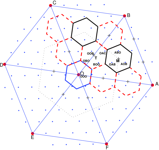
Figure 5: Index assignments (not optimal) by the greedy index assignment algorithm for the $A_{2}$ lattice with index $N=31$, $K=3$. Points of $\Lambda$, $\Lambda_{s}$ and $\Lambda_{s/3}$ are marked by $\cdot$, $\bullet$ and $+$, respectively.

Theorem 2 is concerned with when the two terms of $d_{s}$ in (17) can be minimized independently by the greedy index assignment algorithm. While being mostly true for $K=2$ as stated by the theorem and as we saw in Fig. 2 and Fig. 4 LABEL:secsub:Examples, this may not be guaranteed when $K>2$. Fig. 5 presents the index assignment generated by the greedy algorithm for $K=3$ on $A_{2}$ lattice. The solution is now suboptimal. Indeed, consider the central lattice point in $V_{s/3}(T)$ that is labeled by $OAC$ in Fig. 5, changing the label from $OAC$ to $BOA$ will reduce $d_{s}$ of the central lattice point in question. The change reduces the first term of $d_{s}$, although the second term of $d_{s}$ increases slightly. Note that the $3$-tuple $(O,A,C)$ has centroid $T$, and the $3$-tuple $(B,O,A)$ has centroid $M$.

In order to make up for the loss of optimality by the greedy algorithm, we develop a local adjustment algorithm. If a central lattice point $\lambda$ is labeled by an ordered $K$-tuple that has centroid $\tau\in\Lambda_{s/K}$, we say that $\lambda$ is attracted by site $\tau$. If two Voronoi cells $V_{s/K}(\tau_{1})$ and $V_{s/K}(\tau_{2})$ are spatially adjacent, we say that site $\tau_{1}$ and site $\tau_{2}$ are neighbors. In Figure 5, site $O$ and site $T$ are neighbors, while site $O$ and site $M$ are not neighbors.

Figure 6: Remove lattice $\lambda$ from site $a$, and add it to site $b$

In Fig. 6, assume two neighboring sites $a$ and $b$ attract $m$ and $n$ central lattice points respectively. The $m$ ($n$) central lattice points are labeled by $m$ ($n$) nearest ordered $K$-tuples centered at site $a$ ($b$). For any point $x\in R^{L}$, let $J_{\overrightarrow{ab}}(x)$ be the projection value of $x$ onto the axis $\overrightarrow{ab}$. Consider the set $S(a)$ of all the $m$ points currently attracted by site $a$, and find

$$\lambda_{max}=\arg\max_{\lambda\in S(a)}J_{\overrightarrow{ab}}(\lambda).$$ (56)

Now, introduce an operator $\Rsh(a,b)$ that alters the label of $\lambda_{max}$ to an ordered $K$-tuple of sublattice points centered at $b$. The effect of $\Rsh(a,b)$ is that sites $a$ and $b$ attract $m-1$ and $n+1$ central lattice points respectively, which are respectively labeled by $m-1$ and $n+1$ nearest ordered $K$-tuples centered at site $a$ and site $b$.

¿From the definition of side distortion $d_{s}=\sum_{\lambda\in\Lambda}d(\lambda)P(\lambda)$ in (17), we have

$$d(\lambda)=\left(\frac{1}{K}\sum_{k=1}^{K}{\left\|{\alpha_{k}(\lambda)-\mu(\alpha(\lambda))}\right\|^{2}}\right)+\left(\zeta{\left\|{\lambda-\mu(\alpha(\lambda))}\right\|^{2}}\right).$$ (57)

Let us compute the change of $d(\lambda_{max})$ caused by the operation $\Rsh(a,b)$.

The change in the second term of $d(\lambda_{max})$ is

$$\begin{split}&\zeta\left({\left\|{\lambda_{max}-b}\right\|^{2}-\left\|{\lambda_{max}-a}\right\|^{2}}\right)\\ &=\frac{\zeta}{L}\left(\left({J_{\overrightarrow{ab}}(\lambda_{max})-L\left\|b-a\right\|}\right)^{2}-J_{\overrightarrow{ab}}(\lambda_{max})^{2}\right).\end{split}$$ (58)

Note the change of the second term is positive if $\lambda_{max}\in V_{s/K}(a)$.

The change in the first term is

$$f_{b}(n+1)-f_{a}(m),$$ (59)

where $f_{\tau}(i)$ is the $i^{th}$ smallest value of $\frac{1}{K}\sum_{k=1}^{K}{\left\|{\lambda_{k}-\tau}\right\|^{2}}$ over all ordered $K$-tuples $(\lambda_{1},\lambda_{2},\cdots,\lambda_{K})\in\Lambda_{s}^{K}$ such that $m(\lambda_{1},\lambda_{2},\cdots,\lambda_{K})=\tau$.

The net change in $d(\lambda_{max})$ made by operation $\Rsh(a,b)$ is then

$$\Delta(a,b)=\zeta\left({\left\|{\lambda_{max}-b}\right\|^{2}-\left\|{\lambda_{max}-a}\right\|^{2}}\right)+f_{b}(n+1)-f_{a}(m).$$ (60)

If $\Delta(a,b)<0$, then $\Rsh(a,b)$ improves index assignment.

The preceding discussions lead us to a simple local adjustment algorithm:

$(a^{*},b^{*})=\arg\min_{a\ \mbox{neighbors}\ b}\Delta(a,b)$;
While	$\Delta(a^{*},b^{*})<0$ do
	$\Rsh(a,b)$;
	$(a^{*},b^{*})=\arg\min_{a\ \mbox{neighbors}\ b}\Delta(a,b)$.

Note that it is only necessary to invoke the local adjustment $\Rsh(a,b)$ if the greedy algorithm does not simultaneously minimize the two terms of $d_{s}$.

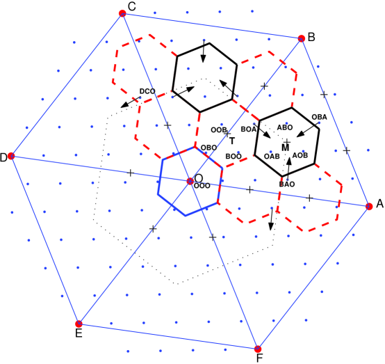
Figure 7: Optimal index assignments for the $A_{2}$ lattice, $N=31$, $K=3$. Points of $\Lambda$, $\Lambda_{s}$ and $\Lambda_{s/3}$ are marked by $\cdot$, $\bullet$ and $+$, respectively.

Fig. 7 shows the result of applying the local adjustment algorithm to the output of the greedy algorithm presented in Fig. 5. It is easy to prove that the local adjustment algorithm indeed finds the optimal index assignment for this case of three description MDLVQ.

Finally, we conjecture that a combined use of the greedy algorithm and local adjustment $\Rsh(a,b)$ solves the problem of optimal MDLVQ index assignment for any $L$-dimensional lattice and for all values of $K$ and $N$.

VIII Conclusion

Although optimal MDLVQ index assignment is conceptually a problem of linear assignment, it involves a bijective mapping between two infinite sets $\Lambda$ and $\Lambda_{s}^{K}$. No good solutions are known to reduce the underlying bipartite graph to a modest size while ensuring optimality. We developed a linear-time algorithm for MDLVQ index assignment, and proved it to be asymptotically (in the sublattice index value $N$) optimal for any $K\geq 2$ balanced descriptions in any dimensions. For two balanced descriptions the optimality holds for finite values of $N$ as well, under some mild conditions. We conjecture that the algorithm, with an appropriate local adjustment, is also optimal for any values of $K$ and $N$.

The optimal index assignment is constructed using a new notion of $K$-fraction lattice. The $K$-fraction lattice also lends us a better tool to analyze and quantify the MDLVQ performance. The expected distortion of optimal MDLVQ is derived in exact closed form for $K=2$ and any $N$. For cases $K>2$, we improved the current asymptotic expression of the expected distortion. These results can be used to determine the optimal values of $K$ and $N$ that minimize the expected MDLVQ distortion, given the total entropy rate and given the loss probability.

References

- [1] V. K. Goyal, “Multiple description coding: compression meets the network,” IEEE Signal Processing Mag., pp. 74–93, Sep. 2001.
- [2] S. D. Servetto, V. A. Vaishampayan, and N. J. A. Sloane, “Multiple description lattice vector quantization,” in IEEE Proc. Data Compression Conf., Mar. 1999, pp. 13–22.
- [3] S. N. Diggavi, N. J. A. Sloane, and V. A. Vaishampayan, “Design of asymmetric multiple description lattice vector quantizers,” in Proc. IEEE Data Compression Conf., Mar. 2000, pp. 490–499.
- [4] V. A. Vaishampayan, N. J. A. Sloane, and S. D. Servetto, “Multiple description vector quantization with lattice codebooks: Design and analysis,” IEEE Trans. Inform. Theory, vol. 47, no. 5, pp. 1718–1734, July 2001.
- [5] S. N. Diggavi, N. J. A. Sloane, and V. A. Vaishampayan, “Asymmetric multiple description lattice vector quantizers,” IEEE Trans. Inform. Theory, vol. 48, no. 1, pp. 174–191, Jan. 2002.
- [6] J. A. Kelner, V. K. Goyal, and J. Kovačević, “Multiple description lattice vector quantization: Variations and extensions,” in Proc. IEEE Data Compression Conf., Mar. 2000, pp. 480–489.
- [7] V. K. Goyal, J. A. Kelner, and J. Kovačević, “Multiple description vector quantization with a coarse lattice,” IEEE Trans. Inform. Theory, vol. 48, pp. 781–788, Mar. 2002.
- [8] C. Tian and S. S. Hemami, “Staggered lattices in multiple description quantization,” in Proc. IEEE Data Compression Conf., Mar. 2005, pp. 398–407.
- [9] J. Østergaard, J. Jensen, and R. Heusdens, “-channel symmetric multiple-description lattice vector quantization,” in Proc. IEEE Data Compression Conf., Mar. 2005, pp. 378–387.
- [10] ——, “-channel entropy-constrained multiple-description lattice vector quantization,” IEEE Trans. Inform. Theory, vol. 52, no. 5, pp. 1956–1973, May 2006.
- [11] V. A. Vaishampayan, “Design of multiple description scalar quantizers,” IEEE Trans. Inform. Theory, vol. 39, pp. 821–834, May 1993.
- [12] T. Y. Berger-Wolf and E. M. Reingold, “Index assignment for multichannel communication under failure,” IEEE Trans. Inform. Theory, vol. 48, no. 10, pp. 2656–2668, Oct. 2002.
- [13] M. Garey, D. S. Johnson, and H. S. Witsenhausen, “The complexity of the generalized lloyd-max problem,” IEEE Trans. Inform. Theory, vol. 28, no. 2, p. 255 C266, Mar. 1982.
- [14] J. H. Conway and N. J. A. Sloane, Sphere Packings, Lattices, and Groups. Springer, 1998.
- [15] J. Hopcroft and R. Karp, “An O() algorithm for maximum matchings in bipartite graphs,” SIAM Journal on Computing, vol. 2, no. 4, pp. 225–231, 1973.
- [16] E. T. Whittaker and G. N. Watson, A Course of Modern Analysis, 4th ed. Camb. Univ. Press, 1963.