Simple Methods For Drawing Rational Surfaces as Four or Six Bézier Patches

Abstract. In this paper, we give several simple methods for drawing a whole rational surface (without base points) as several Bézier patches. The first two methods apply to surfaces specified by triangular control nets and partition the real projective plane $\mathbb{RP}^{2}$ into four and six triangles respectively. The third method applies to surfaces specified by rectangular control nets and partitions the torus $\mathbb{RP}^{1}\times\mathbb{RP}^{1}$ into four rectangular regions. In all cases, the new control nets are obtained by sign flipping and permutation of indices from the original control net. The proofs that these formulae are correct involve very little computations and instead exploit the geometry of the parameter space ($\mathbb{RP}^{2}$ or $\mathbb{RP}^{1}\times\mathbb{RP}^{1}$). We illustrate our method on some classical examples. We also propose a new method for resolving base points using a simple “blowing up” technique involving the computation of “resolved” control nets.

1 Introduction

In this paper, we consider the problem of drawing a whole rational surface. For example, consider the sphere $F$ specified by the fractions

$$x(u,v)=\frac{2u}{u^{2}+v^{2}+1},\quad y(u,v)=\frac{2v}{u^{2}+v^{2}+1},\quad z(u,v)=\frac{u^{2}+v^{2}-1}{u^{2}+v^{2}+1}.$$

The problem is that no matter how large the interval $[r,s]$ is, the trace $F([r,s]\times[r,s])$ of $F$ over $[r,s]\times[r,s]$ is not the trace of the entire surface. In this particular example, we could take advantage of symmetries, but in general, this may not be possible. We could use any of the bijections from $\>]-1,1[\>$ to $\mathbb{R}$ to reduce the parameter domain to the square $[-1,1]\times[-1,1]$, but since these maps are at least quadratic, this could triple the total degree of the surface, leading to an impractical method. For example, using the map

$$t\mapsto\frac{t}{1-t^{2}}$$

$$\hbox{the fraction}\quad\frac{1}{u^{2}+uv}\quad\hbox{becomes}\quad\frac{(1-u^{2})^{2}(1-v^{2})}{(1-v^{2})u^{2}+(1-u^{2})uv}.$$

Recomputing the control net after substitution would also be quite expensive. Indeed, one of the reasons why the problem is not trivial is that in most CAGD applications, the surface is given in terms of control points rather than parametrically (in terms of polynomials).

Thus, the problem is to cope with the situation in which $u$ or $v$ become infinite. But what do we mean exactly by that? To deal with this situation rigorously, we can “go projective”, that is, homogenize the polynomials. However, this can be done in two different ways. The first method is to homogenize with respect to the total degree, replacing $u$ by $u/t$ and $v$ by $v/t$, getting

$$x=\frac{2ut}{u^{2}+v^{2}+t^{2}},\quad y=\frac{2vt}{u^{2}+v^{2}+t^{2}},\quad z=\frac{u^{2}+v^{2}-t^{2}}{u^{2}+v^{2}+t^{2}}.$$

The parameter domain is now the real projective plane $\mathbb{RP}^{2}$. Points at infinity are the points of homogeneous coordinates $(u,v,0)$ (i.e., when $t=0$). Observe that all these point at infinity yield the north pole $(0,0,1)$ on the sphere.

The second method is to homogenize separately in $u$ and $v$, replacing $u$ by $u/t_{1}$ and $v$ by $v/t_{2}$, getting

$$x=\frac{2ut_{1}t_{2}^{2}}{u^{2}t_{2}^{2}+v^{2}t_{1}^{2}+t_{1}^{2}t_{2}^{2}},\quad y=\frac{2vt_{1}^{2}t_{2}}{u^{2}t_{2}^{2}+v^{2}t_{1}^{2}+t_{1}^{2}t_{2}^{2}},\quad z=\frac{u^{2}t_{2}^{2}+v^{2}t_{1}^{2}-t_{1}^{2}t_{2}^{2}}{u^{2}t_{2}^{2}+v^{2}t_{1}^{2}+t_{1}^{2}t_{2}^{2}}.$$

This time, the parameter domain is the product space $\mathbb{RP}^{1}\times\mathbb{RP}^{1}$, where $\mathbb{RP}^{1}$ is the real projective line. The domain $\mathbb{RP}^{1}\times\mathbb{RP}^{1}$ is homeomorphic to a torus, and it is not homeomorphic to $\mathbb{RP}^{2}$. Observe that when $t_{1}=t_{2}=0$, all the numerators and the denominator vanish simultaneously. We have what is called a base point. This is annoying but not terribly surprising, since a sphere is not of the same topological type as a torus. It should be noted that there are also rational surfaces (such as the torus) that do not have base points when treated as surfaces with domain $\mathbb{RP}^{1}\times\mathbb{RP}^{1}$ but have base points when treated as having domain $\mathbb{RP}^{2}$ (see Section 6), and vice versa.

In summary, there are two ways to deal with infinite values of the parameters. We can homogenize with respect to the total degree $m$ (replacing $u$ by $u/t$ and $v$ by $v/t$). This leads to rational surfaces specified by triangular control nets, as we will see more precisely in the next section. The other method is to homogenize with respect to $u$ and the maximum degree $p$ in $u$ (replacing $u$ by $u/t_{1}$) and with respect to $v$ and the maximum degree $q$ in $v$ (replacing $v$ by $v/t_{2}$). This leads to rational surfaces specified by rectangular control nets, as we will see more precisely in the next section.

The problem of drawing a rational surface reduces to the problem of partitioning the parameter domain into simple connected regions $R_{i}$ such as triangles or rectangles, in such a way that there is some prespecified region $R_{0}$ and some projectivities such that every other region is the image of the region $R_{0}$ under one of the projectivities. Furthermore, if the patch associated with the region $R_{0}$ is given by a control net ${\cal N}_{0}$, we want the control net ${\cal N}_{i}$ associated with the region $R_{i}$ to be computable very quickly from ${\cal N}_{0}$.

In the case of the real projective plane $\mathbb{RP}^{2}$, we can use the fact that $\mathbb{RP}^{2}$ is obtained as the quotient of the sphere $S^{2}$ after identification of antipodal points. The real projective plane can be partitioned by projecting any polyhedron inscribed in the sphere $S^{2}$ on a plane. This way of dividing the real projective plane into regions is discussed quite extensively in Hilbert and Cohn-Vossen [14] (see Chapter III). As noted by Hilbert, it is better to use polyhedra with central symmetry, so that the projective plane is covered only once since vertices come in pairs of antipodal points. In particular, we can use the four Platonic solids other than the tetrahedron, but if we want rectangular or triangular regions, only the cube, the octahedron, and the icosahedron can be used. Indeed, projection of the dodecahedron yields pentagonal regions (see Hilbert and Cohn-Vossen [14], page 147-150).

If we project the cube onto one of its faces from its center, we get three rectangular regions (see Section 3). It is easy to find the projectivities that map the central region onto the other two. Since we are dealing with the projective plane, it is better to use triangular control nets to avoid base points, and it is necessary to split the central rectangle into two triangles. Thus, the trace of the rational surface is the union of six patches over various triangles. It is shown in Section 3 how the control nets of the other four patches are easily (and cheaply) obtained from the control nets of the two central triangles.

If we project the octahedron onto one of its faces from its center, we get four triangular regions (see Section 4). This time, it is a little harder to write down the projectivities that map the central triangle $rst$ to the other three triangles $R,S,T$. However it is not necessary to find explicit formulae for these projectivities, and using a geometric argument, we can find very simple formulae to compute the control nets associated with the other three triangles from the control net associated with the central triangle, as shown in Section 4.

Projecting the icosahedron onto one of its faces from its center yields ten triangular regions, but we haven’t found formulae to compute control nets of the other regions from the central triangle. We leave the discovery of such formulae as an open and possibly challenging problem.

Let us now consider the problem of partitioning $\mathbb{RP}^{1}\times\mathbb{RP}^{1}$ into simple regions. Since the projective line $\mathbb{RP}^{1}$ is topologically a circle, a very simple method is to inscribe a rectangle (or a square) in the circle and then project it. One way to do so leads to a partition of $\mathbb{RP}^{1}$ into $[-1,1]$ and $\mathbb{RP}^{1}-]-1,1[$. The corresponding projectivity is $t\mapsto\frac{1}{t}$. Other projections lead to a partition of $\mathbb{RP}^{1}$ into $[r,s]$ and $\mathbb{RP}^{1}-]r,s[$ for any affine frame $(r,s)$. In all cases, the torus is split into four rectangular regions, and there are very simple formulae for computing the control nets of the other three rectangular nets from the control net associated with the patch over $[-1,1]\times[-1,1]$ (or more generally, $[r_{1},s_{1}]\times[r_{2},s_{2}]$), as explained in Section 5.

It should be stressed that it is not necessary to compute explicitly the various projectivities, and that in each case, a simple geometric argument yields the desired formulae for the new control nets. Other methods for drawing rational surfaces were also investigated by Bajaj and Royappa [2, 3] and DeRose [5] and will be discussed in Section 4 and Section 5.

There is a problem with our methods when all the numerators and the denominator vanish simultaneously. In this case, we have what is called a base point. In Section 6, we give a new method for resolving base points (in the case of a rational surface specified by a triangular control net), using a simple “blowing-up” technique based on an idea of Warren [18]. What is new is that we give formulae for computing “resolved” control nets.

It turns out that to give rigorous proofs of our formulae, it is necessary to view rational surfaces as surfaces defined in a suitable projective space in terms of multiprojective maps. We will summarize how to do this in Section 2. The proofs that our formulae are correct involve very little computations and instead exploit the geometry of the parameter space ($\mathbb{RP}^{2}$ or $\mathbb{RP}^{1}\times\mathbb{RP}^{1}$). For the sake of brevity, we do not review how polynomial surfaces are defined in terms of control points. The deep reason why polynomial triangular surface patches can be effectively handled in terms of control points is that multivariate polynomials arise from multiaffine symmetric maps (see Ramshaw [17], Farin [7, 6], Hoschek and Lasser [15], or Gallier [11]).

2 Rational Surfaces and Control Points

Denoting the affine plane $\mathbb{R}^{2}$ as ${\cal P}$, a rational surface $F\colon{\cal P}\rightarrow\mathbb{R}^{n}$ of degree $m$ is specified by some fractions

$$x_{1}(u,v)=\frac{F_{1}(u,v)}{F_{n+1}(u,v)},\quad\ldots\quad,x_{n}(u,v)=\frac{F_{n}(u,v)}{F_{n+1}(u,v)},$$

where $F_{1}(u,v),\ldots,F_{n+1}(u,v)$ are polynomials of total degree $\leq m$. In order to handle rational surfaces in terms of control points, it turns out that it is necessary to view rational surfaces as surfaces in some projective space. Roughly, this means that we have to homogenize the polynomials $F_{1}(u,v),\ldots,F_{n+1}(u,v)$. However, the polar forms of homogeneous polynomials are multilinear, and thus we must deal with multilinear maps rather than multiaffine maps. Fortunately, there is a construction to embed an affine space into a vector space, in such a way that multiaffine maps extend uniquely to multilinear maps. This construction is described in Berger [4] and is at the heart of the presentation of rational surfaces in Fiorot and Jeannin [8, 9]. However, Fiorot and Jeannin do not use polar forms. We have adapted their approach in the framework of polar forms in Gallier [12]. In this paper, we simply review the facts needed to understand the proof of our theorems. Given a vector space $E$, we denote the projective space induced by $E$ as $\mathbb{P}(E)$ (see Berger [4] or Gallier [12]). Given an affine space $E$ with associated vector space $\overrightarrow{E}$, a vector space $\widehat{E}$ can be constructed, such that $E$ is embedded as an affine hyperplane in $\widehat{E}$ via an affine map $j\colon E\rightarrow\widehat{E}$, and $\overrightarrow{E}$ as a hyperplane.

Figure 1: Embedding an affine space into a vector space

Both hyperplanes are defined by some linear form $\omega\colon\widehat{E}\rightarrow\mathbb{R}$. The previous diagram illustrates the embedding of the affine space $E$ into the vector space $\widehat{E}$: Roughly, the vector space $\widehat{E}$ has the property that for any vector space $\overrightarrow{F}$ and any affine map $f\colon E\rightarrow\overrightarrow{F}$, there is a unique linear map $\widehat{f}\colon\widehat{E}\rightarrow\overrightarrow{F}$ extending $f\colon E\rightarrow\overrightarrow{F}$. As a consequence, given two affine spaces $E$ and $F$, every affine map $f\colon E\rightarrow F$ extends uniquely to a linear map $\widehat{f}\colon\widehat{E}\rightarrow\widehat{F}$.

A pair $\langle a,\lambda\rangle$ where $a\in E$ and $\lambda\not=0$ is called a weighted point. Vectors in $\widehat{E}$ of the form $\langle a,1\rangle$ are identified with points $a$ in $E$. It is easily shown that for every $a\in E$, we have $\widehat{E}=\overrightarrow{E}\oplus\mathbb{R}a$.

We have the following important result whose proof can be found in Gallier [12], or inferred from Ramshaw [17].

Lemma 2.1

Given any two affine spaces $E$ and $F$ and a multiaffine map $f\colon E^{m}\rightarrow F$, there is a unique multilinear map $\widehat{f}\colon(\widehat{E})^{m}\rightarrow\widehat{F}$ extending $f$ as in the diagram below:

Given an affine space $E$, the projective space $\mathbb{P}(\widehat{E})$ induced by $\widehat{E}$ is denoted as $\widetilde{E}$, and it is called the projective completion of $E$. Observe that $\widetilde{\mathbb{R}}=\mathbb{RP}^{1}$ and $\widetilde{{\cal P}}=\mathbb{RP}^{2}$.

The upshot of the above considerations is that a rational surface can be defined in terms of multilinear maps. Let ${\cal E}$ be some ambiant affine space in which our surfaces live, in most cases $\mathbb{R}^{3}$. If we first homogenize the polynomials $F_{i}(u,v)$ with respect to the total degree $m$ (replacing $u$ by $u/z$ and $v$ by $v/z$), we can view a rational surface as a map

$$F\colon\widetilde{{\cal P}}\rightarrow\widetilde{{\cal E}}$$

(where ${\cal P}=\mathbb{R}^{2}$ is the affine plane) induced by some symmetric multilinear map

$$f\colon(\widehat{{\cal P}})^{m}\rightarrow\widehat{{\cal E}}$$

such that

$$F([u,v,z])=\mathbb{P}(f)(\underbrace{(u,v,z),\ldots,(u,v,z)}_{m}),$$

for all homogeneous coordinates $(u,v,z)\in\mathbb{R}^{3}$. We call such surfaces rational total degree surfaces, or triangular rational surfaces. Furthermore, for any affine frame $\Delta rst$, the triangular control net ${\cal N}=(\theta_{i,\,j,\,k})_{(i,j,k)\in\Delta_{m}}$ (in $\widehat{{\cal E}}$) w.r.t. $\Delta rst$ defining the triangular surface $F$ is given by the formulae

$$\theta_{i,\,j,\,k}=f(\underbrace{r,\ldots,r}_{i},\underbrace{s,\ldots,s}_{j},\underbrace{t,\ldots,t}_{k}),\quad\hbox{where}\>i+j+k=m.$$

On the other hand, if we first homogenize the polynomials $F_{i}(u,v)$ with respect to $u$ and the maximum degree $p$ in $u$ (replacing $u$ by $u/t_{1}$) and second with respect to $v$ and the maximum degree $q$ in $v$ (replacing $v$ by $v/t_{2}$), we can view a rational surface as a map

$$F\colon\widetilde{\mathbb{R}}\times\widetilde{\mathbb{R}}\rightarrow\widetilde{{\cal E}}$$

induced by some multilinear map

$$f\colon(\widehat{\mathbb{R}})^{p}\times(\widehat{\mathbb{R}})^{q}\rightarrow\widehat{{\cal E}}$$

which is symmetric in its first $p$ arguments and in its last $q$ arguments, and such that

$$F([u,t_{1}],[v,t_{2}])=\mathbb{P}(f)(\underbrace{(u,t_{1}),\ldots,(u,t_{1})}_{p},\underbrace{(v,t_{2}),\ldots,(v,t_{2})}_{q}),$$

for all homogeneous coordinates $(u,t_{1}),(v,t_{2})\in\mathbb{R}^{2}$. We call such surfaces rational surfaces of bidegree $\langle p,q\rangle$, or rectangular rational surfaces. Furthermore, given any two affine frames $(r_{1},s_{1})$ and $(r_{2},s_{2})$ for the affine line $\mathbb{R}$, the rectangular control net ${\cal N}=(\theta_{i,\,j})_{0\leq i\leq p,\,0\leq j\leq q}$ (in $\widehat{{\cal E}}$) w.r.t. $(r_{1},s_{1})$ and $(r_{2},s_{2})$ defining the rectangular surface $F$ is given by the formulae

$$\theta_{i,\,j}=f(\underbrace{r_{1},\ldots,r_{1}}_{p-i},\underbrace{s_{1},\ldots,s_{1}}_{i},\underbrace{r_{2},\ldots,r_{2}}_{q-j},\underbrace{s_{2},\ldots,s_{2}}_{j}).$$

A base point of a rational surface $F$ specified by a multilinear map $f$ is any point $a\in\mathbb{R}^{3}$ such that $f(\underbrace{a,\ldots,a}_{m})=\overrightarrow{0}$, or any point $(u,v)\in\mathbb{R}^{2}$ such that $f(\underbrace{u,\ldots,u}_{p},\underbrace{v,\ldots,v}_{q})=\overrightarrow{0}$.

3 Splitting Triangular Rational Surfaces Into Six Triangular Patches

As we explained in Section 1, if we project a cube onto one of its faces from its center, we obtain a partition of the projective plane $\mathbb{RP}^{2}$ into three rectangular regions, in such a way that there exist simple projectivities $\varphi$ and $\psi$ between the square $[-1,1]\times[-1,1]$ and the other two regions.

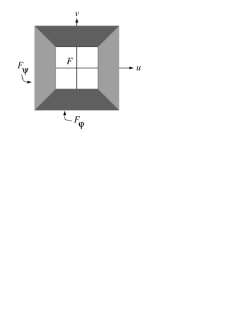
Figure 2: Dividing the projective plane into $3$ rectangular regions

The projectivity $\varphi$ is induced by the linear isomorphism of $\mathbb{R}^{3}$ given by

$$(u,v,w)\mapsto(v,w,u).$$

Choosing the line at infinity $w=0$, the restriction of this map to the affine plane ${\cal P}$ (corresponding to $w=1$) is the map $(u,v,1)\mapsto(v,1,u)$. This is the map from ${\cal P}$ to $\widetilde{{\cal P}}$ such that $(u,v)\mapsto(v/u,1/u)$ if $u\not=0$, and $(0,v)\mapsto(v,1,0)$ when $u=0$. The projectivity $\psi$ is induced by the linear isomorphism of $\mathbb{R}^{3}$ given by

$$(u,v,w)\mapsto(w,u,v).$$

Choosing the line at infinity $w=0$, the restriction of this map to the affine plane ${\cal P}$ (corresponding to $w=1$) is the map $(u,v,1)\mapsto(1,u,v)$. This is the map from ${\cal P}$ to $\widetilde{{\cal P}}$ such that $(u,v)\mapsto(1/v,u/v)$ if $v\not=0$, and $(u,0)\mapsto(1,u,0)$ when $v=0$.

Actually, it turns out that the method of this section holds for any region defined by a nondegenerate quadrilateral $(a,b,c,d)$, i.e. when $(a,b,c,d)$ is a projective frame. However, the details are a bit messy, and for simplicity, we restrict out attention to a rectangular region $[r_{1},s_{1}]\times[r_{2},s_{2}]$. Since we are dealing with triangular surfaces, it will be necessary to split the rectangle $[r_{1},s_{1}]\times[r_{2},s_{2}]$ into two triangles, and thus, we will obtain the trace of a rational surface as the union of $6$ patches over various triangles in the rectangle $[r_{1},s_{1}]\times[r_{2},s_{2}]$. Letting $a,b,c,d$ be the vertices of the rectangle $[r_{1},s_{1}]\times[r_{2},s_{2}]$ defined such that

$$a=(s_{1},s_{2}),\quad b=(r_{1},s_{2}),\quad c=(r_{1},r_{2}),\quad d=(s_{1},r_{2}),$$

as shown below

Figure 3: Some affine frames associated with the rectangle $(a,b,c,d)$

we will consider the following affine frames

$$\openup 3.0pt\halign to=0.0pt{\hfil$\displaystyle{#}$&$\displaystyle{{}#}$\hfil&\llap{$#$}\cr\Delta bca &= ((r_{1}, s_{2}),\> (r_{1}, r_{2}),\> (s_{1}, s_{2})),\cr\Delta dac &= ((s_{1}, r_{2}),\> (s_{1}, s_{2}),\> (r_{1}, r_{2})),\cr\Delta bad &= ((r_{1}, s_{2}),\> (s_{1}, s_{2}),\> (s_{1}, r_{2})).\cr}$$

In particular, a rectangular surface patch defined over the rectangle $[r_{1},s_{1}]\times[r_{2},s_{2}]$ will be treated as the union of two triangular surface patches defined over the triangles $\Delta bca$ and $\Delta dac$. It is somewhat unfortunate that a control net over the third frame $\Delta bad$ needs to be computed, but that is what the proof of lemma 3.2 shows. In any case, such a control net can be computed very cheaply from a control net over $\Delta bca$ (or $\Delta dac$).

There is simple geometric explanation of the partitioning method in terms of the usual model of the real projective plane $\widetilde{{\cal P}}=\mathbb{RP}^{2}$ in $\mathbb{R}^{3}$. Recall that in this model, the real projective plane $\mathbb{RP}^{2}$ consists of the points in the plane $z=1$ corresponding to the lines through the origin not in the plane $z=0$, and of the points at infinity corresponding to the lines through the origin in the plane $z=0$. We view the vertices of the rectangle $(a,b,c,d)$ defined above as points in the plane $z=1$, in which case their coordinates are $(s_{1},s_{2},1)$, $(r_{1},s_{2},1)$, $(r_{1},r_{2},1)$, and $(s_{1},r_{2},1)$. Then, we have the parallelepiped $(a,b,c,d,-a,-b,-c,-d)$. There is a unique projectivity $\mathbb{P}(\varphi)$ such that

$$\mathbb{P}(\varphi)(a)=a,\quad\mathbb{P}(\varphi)(b)=c,\quad\mathbb{P}(\varphi)(c)=d,\quad\mathbb{P}(\varphi)(d)=b.$$

For instance, it is induced by the unique linear map $\varphi$ such that

$$\varphi(a)=a,\quad\varphi(b)=-c,\quad\varphi(c)=-d.$$

Since $d=-b+a+c$, we get

$$\varphi(d)=-\varphi(b)+\varphi(a)+\varphi(c)=c+a-d=(r_{1},s_{2},1)=b.$$

The linear map $\varphi$ transforms the top face $(a,b,c,d)$ of the parallelepiped to the back face $(a,-c,-d,b)$. When a line $L$ through the origin and passing through a point of the face $(a,-c,-d,b)$ varies, the intersection of $L$ with the plane $z=1$ varies in $\varphi([r_{1},s_{1}]\times[r_{2},s_{2}])$. We can define a rhombus $(a,e,f,g,-a,-e,-f,-g)$ inscribed in the sphere of center $O=(0,0,0)$ and of radius $R=\sqrt{s_{1}^{2}+s_{2}^{2}+1}$ passing through $a$, as follows: the points $e,f,g$ are on the upper half-sphere and they are determined by the intersection of the lines $(O,b)$, $(O,c)$ and $(O,d)$ with the sphere. Then, it is obvious that under the central projection of center $O$ onto the plane $z=1$, the top face $(a,e,f,g)$ of the rhombus projects onto the face $(a,b,c,d)$ of the parallelepiped, and that the projection of the rhombus onto the plane $z=1$ yields the desired partitioning of $\mathbb{RP}^{2}$.

Similarly, there is a unique projectivity $\mathbb{P}(\psi)$ such that

$$\mathbb{P}(\psi)(a)=a,\quad\mathbb{P}(\psi)(b)=d,\quad\mathbb{P}(\psi)(c)=b,\quad\mathbb{P}(\psi)(d)=c.$$

It is induced by the unique linear map $\psi$ such that

$$\psi(a)=a,\quad\psi(b)=d,\quad\psi(c)=-b.$$

Since $d=-b+a+c$, we get

$$\psi(d)=-\psi(b)+\psi(a)+\psi(c)=-d+a-b=(-r_{1},-r_{2},-1)=-c.$$

The linear map $\psi$ transforms the top face $(a,b,c,d)$ of the parallelepiped to the right face $(a,d,-b,-c)$. When a line $L$ through the origin and passing through a point of the face $(a,d,-b,-c)$ varies, the intersection of $L$ with the plane $z=1$ varies in $\psi([r_{1},s_{1}]\times[r_{2},s_{2}])$. Again, it is obvious that under the central projection of center $O$ onto the plane $z=1$, the top face $(a,e,f,g)$ of the rhombus projects onto the face $(a,b,c,d)$ of the parallelepiped, and that the projection of the rhombus onto the plane $z=1$ yields the desired partitioning of $\mathbb{RP}^{2}$. Figure 4 shows the parallelepiped $(a,b,c,d,-a,-b,-c,-d)$ and the rhombus $(a,e,f,g,-a,-e,-f,-g)$.

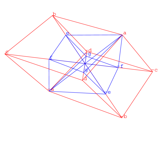
Figure 4: Parallelepiped and rhombus associated with $(a,b,c,d)$

We will now use the maps $\varphi$ and $\psi$ to show how the trace of a rational surface $F$ can be obtained as the union of the traces of three rational surfaces over the rectangle $[r_{1},s_{1}]\times[r_{2},s_{2}]$. The first of these surfaces is $F$ itself, and the two other rational surfaces $F_{\varphi}$ and $F_{\psi}$ are easily obtained from $F$. However, depending on the multilinear map $f$ defining $F$, the surface $F$ (and thus, $F_{\varphi}$ and $F_{\psi}$) may have base points, that is, we may have

$$f(\underbrace{(u,v,z),\ldots,(u,v,z)}_{m})=\overrightarrow{0}$$

for some $(u,v,z)\not=(0,0,0)$. We will show how to deal with this situation later on.

In order to render the trace of $F$, we will use the fact that it is the union of the six traces $F(\Delta bca)$, $F(\Delta dac)$, $F(\varphi(\Delta bca))$, $F(\varphi(\Delta dac))$, $F(\psi(\Delta bca))$, and $F(\psi(\Delta dac))$. Furthermore, the last four traces are also obtained as traces of $F_{\varphi}$ and $F_{\psi}$ over some appropriate choice of affine frames among $\Delta bca$, $\Delta dac$, and $\Delta bad$.

We now show how $F_{\varphi}$ and $F_{\psi}$ are defined, and how their control points can be computed very simply from the control points of $F$ (computed with respect to the affine frames $\Delta bca$, $\Delta dac$, and $\Delta bad$). We will assume that the homogenization $\widehat{{\cal P}}$ of the affine plane ${\cal P}$ is identified with the direct sum $\mathbb{R}^{2}\oplus\mathbb{R}O$, where $O=(0,0)$. Then, every element of $\widehat{{\cal P}}$ is of the form $(u,v,z)\in\mathbb{R}^{3}$.

Definition 3.1

Given an affine space ${\cal E}$ of dimension $\geq 3$, for every rational surface $F\colon\widetilde{{\cal P}}\rightarrow\widetilde{{\cal E}}$ of degree $m$ specified by some symmetric multilinear map $f\colon(\widehat{{\cal P}})^{m}\rightarrow\widehat{{\cal E}}$, the symmetric multilinear maps $f_{\varphi}\colon(\widehat{{\cal P}})^{m}\rightarrow\widehat{{\cal E}}$ and $f_{\psi}\colon(\widehat{{\cal P}})^{m}\rightarrow\widehat{{\cal E}}$ are defined such that

$$\openup 3.0pt\halign to=0.0pt{\hfil$\displaystyle{#}$&$\displaystyle{{}#}$\hfil&\llap{$#$}\cr f_{\varphi}((u_{1}, v_{1}, w_{1}), \ldots,(u_{m}, v_{m}, w_{m})) &= f(\varphi(u_{1},\> v_{1},\> w_{1}), \ldots, \varphi(u_{m},\> v_{m},\> w_{m})),\cr f_{\psi}((u_{1}, v_{1}, w_{1}), \ldots,(u_{m}, v_{m}, w_{m})) &= f(\psi(u_{1},\> v_{1},\> w_{1}), \ldots, \psi(u_{m},\> v_{m},\> w_{m})).\cr}$$

Let $F_{\varphi}\colon\widetilde{{\cal P}}\rightarrow\widetilde{{\cal E}}$ be the rational surface specified by $f_{\varphi}\colon(\widehat{{\cal P}})^{m}\rightarrow\widehat{{\cal E}}$, and let $F_{\psi}\colon\widetilde{{\cal P}}\rightarrow\widetilde{{\cal E}}$ be the rational surface specified by $f_{\psi}\colon(\widehat{{\cal P}})^{m}\rightarrow\widehat{{\cal E}}$.

Observe that the base points of $F_{\varphi}$, if any, have coordinates $(u,v,w)\not=(0,0,0)$ such that

$$f(\varphi(u,\>v,\>w),\ldots,\varphi(u,\>v,\>w))=\overrightarrow{0},$$

and that the base points of $F_{\psi}$, if any, have coordinates $(u,v,w)\not=(0,0,0)$ such that

$$f(\psi(u,\>v,\>w),\ldots,\psi(u,\>v,\>w))=\overrightarrow{0}.$$

Lemma 3.2

Given an affine space ${\cal E}$ of dimension $\geq 3$, for every rational surface $F\colon\widetilde{{\cal P}}\rightarrow\widetilde{{\cal E}}$ of degree $m$ specified by some symmetric multilinear map $f\colon(\widehat{{\cal P}})^{m}\rightarrow\widehat{{\cal E}}$, if $f_{\varphi}$ and $f_{\psi}$ are the symmetric multilinear maps of definition 3.1, except for base points, $F$, $F_{\varphi}$ and $F_{\psi}$ have the same trace. The trace of $F_{\varphi}$ over $\Delta bca$ is the trace of $F$ over $\varphi(\Delta bca)$, the trace of $F_{\varphi}$ over $\Delta dac$ is the trace of $F$ over $\varphi(\Delta dac)$, the trace of $F_{\psi}$ over $\Delta bca$ is the trace of $F$ over $\psi(\Delta bca)$, and the trace of $F_{\psi}$ over $\Delta dac$ is the trace of $F$ over $\psi(\Delta dac)$. Furthermore, if the control nets (in $\widehat{{\cal E}}$) of the surface $F$ w.r.t. the affine frames $\Delta bca$, $\Delta dac$, and $\Delta bad$, are respectively

$$\openup 3.0pt\halign to=0.0pt{\hfil$\displaystyle{#}$&$\displaystyle{{}#}$\hfil&\llap{$#$}\cr\alpha&= (\alpha_{i,\,j,\,k})_{(i,j,k)\in\Delta_{m}},\cr\beta&= (\beta_{i,\,j,\,k})_{(i,j,k)\in\Delta_{m}},\cr\gamma&= (\gamma_{i,\,j,\,k})_{(i,j,k)\in\Delta_{m}},\cr}$$

the control nets $\theta^{1}$ and $\theta^{2}$ (in $\widehat{{\cal E}}$) of the surface $F_{\varphi}$ w.r.t. the affine frames $\Delta bca$ and $\Delta dac$, and the control nets $\rho^{1}$ and $\rho^{2}$ (in $\widehat{{\cal E}}$) of the surface $F_{\psi}$ w.r.t. the affine frame $\Delta bca$ and $\Delta dac$, are given by the equations

$$\openup 3.0pt\halign to=0.0pt{\hfil$\displaystyle{#}$&$\displaystyle{{}#}$\hfil&\llap{$#$}\cr\theta_{i,\, j,\, k}^{1} &= (-1)^{i + j}\> \beta_{j,\, k,\, i},\cr\theta_{i,\, j,\, k}^{2} &= (-1)^{k}\> \gamma_{i,\, j,\, k},\cr\rho_{i,\, j,\, k}^{1} &= (-1)^{j}\> \gamma_{j,\, k,\, i},\cr\rho_{i,\, j,\, k}^{2} &= (-1)^{i + k}\> \alpha_{k,\, i,\, j}.\cr}$$

Proof. We have

$$f_{\varphi}((u_{1},v_{1},w_{1}),\ldots,(u_{m},v_{m},w_{m}))=f(\varphi(u_{1},v_{1},w_{1}),\ldots,\varphi(u_{m},v_{m},w_{m})),$$

and thus

$$\mathbb{P}(f_{\varphi})([u_{1},v_{1},w_{1}],\ldots,[u_{m},v_{m},w_{m}])=\mathbb{P}(f)([\varphi(u_{1},v_{1},w_{1})],\ldots,[\varphi(u_{m},v_{m},w_{m})]).$$

In view of the properties of $\varphi$, it is clear that $F$ and $F_{\varphi}$ have the same trace (except for base points), and that the trace of $F_{\varphi}$ over $\Delta bca$ is the trace of $F$ over $\varphi(\Delta bca)$, and the trace of $F_{\varphi}$ over $\Delta dac$ is the trace of $F$ over $\varphi(\Delta dac)$. A similar argument applies to $F$ and $F_{\psi}$. The formulae for computing the control points of $F_{\varphi}$ w.r.t. the triangle $\Delta bca$ are obtained by computing

$$f_{\varphi}(\underbrace{b,\ldots,b}_{i},\underbrace{c,\ldots,c}_{j},\underbrace{a,\ldots,a}_{k}).$$

Since

$$f_{\varphi}((u_{1},v_{1},w_{1}),\ldots,(u_{m},v_{m},w_{m}))=f(\varphi(u_{1},\>v_{1},\>w_{1}),\ldots,\varphi(u_{m},\>v_{m},\>w_{m})),$$

$\varphi(b)=-c$, $\varphi(c)=-d$, and $\varphi(a)=a$, we have

$$f_{\varphi}(\underbrace{b,\ldots,b}_{i},\underbrace{c,\ldots,c}_{j},\underbrace{a,\ldots,a}_{k})=f(\underbrace{-c,\ldots,-c}_{i},\underbrace{-d,\ldots,-d}_{j},\underbrace{a,\ldots,a}_{k}),$$

that is

$$f_{\varphi}(\underbrace{b,\ldots,b}_{i},\underbrace{c,\ldots,c}_{j},\underbrace{a,\ldots,a}_{k})=(-1)^{i+j}f(\underbrace{c,\ldots,c}_{i},\underbrace{d,\ldots,d}_{j},\underbrace{a,\ldots,a}_{k}),$$

and since the control points $\beta_{i,\,j,\,k}$ are computed w.r.t. the triangle $\Delta dac$, we get

$$\theta_{i,\,j,\,k}^{1}=(-1)^{i+j}\>\beta_{j,\,k,\,i}.$$

The formulae for computing the control points of $F_{\varphi}$ w.r.t. the triangle $\Delta dac$ are obtained by computing

$$f_{\varphi}(\underbrace{d,\ldots,d}_{i},\underbrace{a,\ldots,a}_{j},\underbrace{c,\ldots,c}_{k}).$$

Since

$$f_{\varphi}((u_{1},v_{1},w_{1}),\ldots,(u_{m},v_{m},w_{m}))=f(\varphi(u_{1},\>v_{1},\>w_{1}),\ldots,\varphi(u_{m},\>v_{m},\>w_{m})),$$

$\varphi(d)=b$, $\varphi(c)=-d$, and $\varphi(a)=a$, we have

$$f_{\varphi}(\underbrace{d,\ldots,d}_{i},\underbrace{a,\ldots,a}_{j},\underbrace{c,\ldots,c}_{k})=f(\underbrace{b,\ldots,b}_{i},\underbrace{a,\ldots,a}_{j},\underbrace{-d,\ldots,-d}_{k}),$$

that is

$$f_{\varphi}(\underbrace{d,\ldots,d}_{i},\underbrace{a,\ldots,a}_{j},\underbrace{c,\ldots,c}_{k})=(-1)^{k}f(\underbrace{b,\ldots,b}_{i},\underbrace{a,\ldots,a}_{j},\underbrace{d,\ldots,d}_{k}),$$

and since the control points $\gamma_{i,\,j,\,k}$ are computed w.r.t. the triangle $\Delta bad$, we get

$$\theta_{i,\,j,\,k}^{2}=(-1)^{k}\>\gamma_{i,\,j,\,k}.$$

The formulae for computing the control points of $F_{\psi}$ w.r.t. the triangle $\Delta bca$ are obtained by computing

$$f_{\psi}(\underbrace{b,\ldots,b}_{i},\underbrace{c,\ldots,c}_{j},\underbrace{a,\ldots,a}_{k}).$$

Since

$$f_{\psi}((u_{1},v_{1},w_{1}),\ldots,(u_{m},v_{m},w_{m}))=f(\psi(u_{1},\>v_{1},\>w_{1}),\ldots,\psi(u_{m},\>v_{m},\>w_{m})),$$

$\psi(b)=d$, $\psi(c)=-b$, and $\psi(a)=a$, we have

$$f_{\psi}(\underbrace{b,\ldots,b}_{i},\underbrace{c,\ldots,c}_{j},\underbrace{a,\ldots,a}_{k})=f(\underbrace{d,\ldots,d}_{i},\underbrace{-b,\ldots,-b}_{j},\underbrace{a,\ldots,a}_{k}),$$

that is

$$f_{\psi}(\underbrace{b,\ldots,b}_{i},\underbrace{c,\ldots,c}_{j},\underbrace{a,\ldots,a}_{k})=(-1)^{j}f(\underbrace{d,\ldots,d}_{i},\underbrace{b,\ldots,b}_{j},\underbrace{a,\ldots,a}_{k}),$$

and since the control points $\gamma_{i,\,j,\,k}$ are computed w.r.t. the triangle $\Delta bad$, we get

$$\rho_{i,\,j,\,k}^{1}=(-1)^{j}\>\gamma_{j,\,k,\,i}.$$

Finally, the formulae for computing the control points of $F_{\psi}$ w.r.t. the triangle $\Delta dac$ are obtained by computing

$$f_{\psi}(\underbrace{d,\ldots,d}_{i},\underbrace{a,\ldots,a}_{j},\underbrace{c,\ldots,c}_{k}).$$

Since

$$f_{\psi}((u_{1},v_{1},w_{1}),\ldots,(u_{m},v_{m},w_{m}))=f(\psi(u_{1},\>v_{1},\>w_{1}),\ldots,\psi(u_{m},\>v_{m},\>w_{m})),$$

$\psi(d)=-c$, $\psi(c)=-b$, and $\psi(a)=a$, we have

$$f_{\psi}(\underbrace{d,\ldots,d}_{i},\underbrace{a,\ldots,a}_{j},\underbrace{c,\ldots,c}_{k})=f(\underbrace{-c,\ldots,-c}_{i},\underbrace{a,\ldots,a}_{j},\underbrace{-b,\ldots,-b}_{k}),$$

that is

$$f_{\psi}(\underbrace{d,\ldots,d}_{i},\underbrace{a,\ldots,a}_{j},\underbrace{c,\ldots,c}_{k})=(-1)^{i+k}f(\underbrace{c,\ldots,c}_{i},\underbrace{a,\ldots,a}_{j},\underbrace{b,\ldots,b}_{k}),$$

and since the control points $\alpha_{i,\,j,\,k}$ are computed w.r.t. the triangle $\Delta bca$, we get

$$\rho_{i,\,j,\,k}^{2}=(-1)^{i+k}\>\alpha_{k,\,i,\,j}.$$

     

The above calculations show that $\varphi$ and $\psi$ can be defined as above provided that $d=-b+a+c$, or equivalently $b+d=a+c$, which means that $(a,b,c,d)$ is a parallelogram. Actually, lemma 3.2 also holds in the more general situation where $(a,b,c,d)$ is a projective frame, i.e. a quadrilateral whose vertices are in general position. However, the definition of the linear maps $\varphi$ and $\psi$ is a little more messy. As before, we identify $a,b,c,d$ with points in the plane $z=1$, and we let $a=(a_{1},a_{2},1)$, $b=(b_{1},b_{2},1)$, $c=(c_{1},c_{2},1)$, and $d=(d_{1},d_{2},1)$. To find a linear map $\varphi$ inducing the unique projectivity $\mathbb{P}(\varphi)$ such that

$$\mathbb{P}(\varphi)(a)=a,\quad\mathbb{P}(\varphi)(b)=c,\quad\mathbb{P}(\varphi)(c)=d,\quad\mathbb{P}(\varphi)(d)=b,$$

we let $d=\lambda a+\mu b+\nu c$ and $b=\lambda^{\prime}a+\mu^{\prime}c+\nu^{\prime}d$, where $\lambda+\mu+\nu=1$ and $\lambda^{\prime}+\mu^{\prime}+\nu^{\prime}=1$, and $\varphi$ is the unique linear map such that

$$\varphi(\lambda a)=\lambda^{\prime}a,\quad\varphi(\mu b)=\mu^{\prime}c,\quad\varphi(\nu c)=\nu^{\prime}d.$$

Then, $\varphi(d)=b$, as desired. The linear map $\psi$ can be defined in a similar way. The proof still goes through since the maps involved are multilinear, and thus not disturbed by scalar multiples.

Lemma 3.2 shows that in order to render a rational surface, provided that it does not have base points, we just need to compute the control nets $\alpha,\beta,\gamma$ for the surface $F$ w.r.t. the affine frames $\Delta bca$, $\Delta dac$, and $\Delta bad$, since then, the control nets $\theta^{1}$ and $\theta^{2}$ (in $\widehat{{\cal E}}$) of the surface $F_{\varphi}$ w.r.t. the affine frames $\Delta bca$ and $\Delta dac$, and the control nets $\rho^{1}$ and $\rho^{2}$ (in $\widehat{{\cal E}}$) of the surface $F_{\psi}$ w.r.t. the affine frame $\Delta bca$ and $\Delta dac$, are obtained at trivial cost.

Remark: It should be noted that the surface patches associated with the control nets $\alpha$, $\beta$, $\theta^{1}$, $\theta^{2}$, $\rho^{1}$, and $\rho^{2}$, may overlap in more than boundaries. In fact, there are examples where $\alpha$ and $\beta$ determine the entire surface, and other examples in which $\theta^{1}$, $\theta^{2}$, $\rho^{1}$, and $\rho^{2}$, determine the entire surface.

It is fairly easy to implement this method in Mathematica. The interested reader will find such an implementation in Gallier [12]. In the interest of brevity, we content ourselves with some examples.

Example 1. The algorithm is illustrated by the following example of an ellipsoid defined by the fractions

$$x(u,v)=\frac{2c_{1}u}{u^{2}+v^{2}+1},\quad y(u,v)=\frac{2c_{2}v}{u^{2}+v^{2}+1},\quad z(u,v)=\frac{c_{3}(u^{2}+v^{2}-1)}{u^{2}+v^{2}+1}.$$

It is easily verified that this representation of the ellipsoid is derived from the stereographic projection from the north pole onto the plane $z=0$. The coordinates of a point on the sphere are the coordinates of the image of a point $(u,v)$ the $xOy$ plane, under the inverse of stereographic projection. We leave as an exercise to show that the following triangular control net for $c_{1}=4$, $c_{2}=3$, $c_{3}=2$, is obtained:

net = {{0, 0, -2, 1}, {0, 3, -2, 1}, {0, 3, 0, 2},
       {4, 0, -2, 1}, {4, 3, -2, 1}, {4, 0, 0, 2}}

The following picture shows the result of iterating the subdivision algorithm $3$ times on the nets net1 and net2:

Figure 5: Patches 1, 2, of an ellipsoid

Iterating the subdivision algorithm $3$ times on the nets theta1 and theta2 yields:

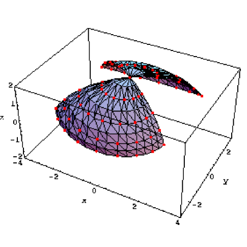
Figure 6: Patches 3, 4, of an ellipsoid

Iterating the subdivision algorithm $3$ times on the nets rho1 and rho2 yields:

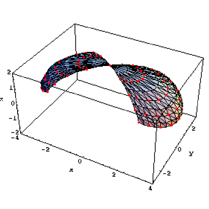
Figure 7: Patches 5, 6, of an ellipsoid

The result of putting all these patches together is the entire ellipsoid:

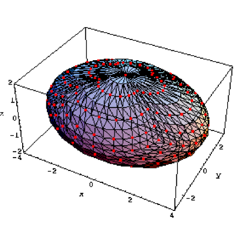
Figure 8: An entire ellipsoid

Of course, we could have taken advantage of symmetries, and our point is to illustrate the algorithm.

Example 2. The Steiner roman surface is the surface of implicit equation

$$x^{2}y^{2}+y^{2}z^{2}+x^{2}z^{2}=2xyz.$$

It is easily verified that the following parameterization works:

$$x(u,v)=\frac{2v}{u^{2}+v^{2}+1},\quad y(u,v)=\frac{2u}{u^{2}+v^{2}+1},\quad z(u,v)=\frac{2uv}{u^{2}+v^{2}+1}.$$

It can be shown that this surface is contained inside the tetrahedron defined by the planes

$$-x+y+z=1,\quad x-y+z=1,\quad x+y-z=1,\quad-x-y-z=1,$$

with $-1\leq x,y,z\leq 1$. The surface touches these four planes along ellipses, and at the middle of the six edges of the tetrahedron, it has sharp edges. Furthermore, the surface is self-intersecting along the axes, and is has four closed chambers. A more extensive discussion can be found in Hilbert and Cohn-Vossen [14], in particular, its relationship to the heptahedron. A triangular control net is easily obtained:

stein1 = {{0, 0, 0, 1}, {1, 0, 0, 1}, {1, 0, 0, 2},
       {0, 1, 0, 1}, {1, 1, 1, 1},  {0, 1, 0, 2}};

We can display the entire surface using the method described in this section. Indeed, all six patches are needed to obtain the entire surface. One view of the surface obtained by subdividing $3$ times is shown below (see Figure 9). Patches 1 and 2 are colored blue, patches 3 and 4 are colored red, and patches 5 and 6 are colored green. A closer look reveals that the three colored patches are identical under appropriate rigid motions, and fit perfectly.

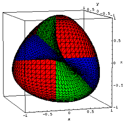
Figure 9: The Steiner roman surface

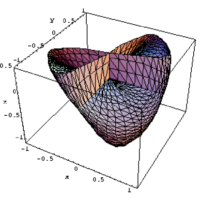
Figure 10: A cut of the Steiner roman surface

Another revealing view (see Figure 10) is obtained by cutting off a top portion of the surface. This way, it is clear that the surface has chambers.

4 Splitting Triangular Rational Surfaces Into Four Triangular Patches

As explained in Section 1, we obtain a partition of the real projective plane $\mathbb{RP}^{2}$ into four triangles if we project an octahedron onto one of its faces from its center. We sketch such a method, leaving the simple details to the reader.

Figure 11: Splitting $\mathbb{RP}^{2}$ into four triangles

We let $r,s,t$ be the vertices of the central triangle. The four triangles defined by the lines $\langle r,s\rangle$, $\langle s,t\rangle$, and $\langle r,t\rangle$ are denoted as $rst$, $R$, $S$, and $T$, where $R,S,T$ contain points at infinity. It is easy to find three projectivities $\varphi_{i}\colon\mathbb{RP}^{2}\rightarrow\mathbb{RP}^{2}$, $i=1,2,3$, such that $\varphi_{1}(rst)=R$, $\varphi_{2}(rst)=S$, and $\varphi_{3}(rst)=T$. Then, we get some rational surfaces $F_{i}=F\circ\varphi_{i}$, $i=1,2,3$. Indeed, if we use the model of $\mathbb{RP}^{2}$ in $\mathbb{R}^{3}$ where the points $r,s,t$ are considered as being in the plane $z=1$, it is immediately verified that the linear maps

$$\openup 3.0pt\halign to=0.0pt{\hfil$\displaystyle{#}$&$\displaystyle{{}#}$\hfil&\llap{$#$}\cr(r, s, t) &\mapsto(-r, s, t),\cr(r, s, t) &\mapsto(r, -s, t),\cr(r, s, t) &\mapsto(r, s, -t),\cr}$$

induce $\varphi_{1},\varphi_{2},\varphi_{3}$. Furthermore, if the control net (in $\widehat{{\cal E}}$) of the triangular surface $F$ w.r.t. the affine frame $\Delta rst$ is $\alpha=(\alpha_{i,\,j,\,k})_{(i,j,k)\in\Delta_{m}}$, it can be shown that the control nets $\theta^{1},\theta^{2}$, and $\theta^{3}$ of the surfaces $F_{1},F_{2},F_{3}$ w.r.t. $\Delta rts$ are given by the formulae

$$\openup 3.0pt\halign to=0.0pt{\hfil$\displaystyle{#}$&$\displaystyle{{}#}$\hfil&\llap{$#$}\cr\theta^{1}_{i,\, j,\, k} &= (-1)^{i} \alpha_{i,\, j,\, k},\cr\theta^{2}_{i,\, j,\, k} &= (-1)^{j} \alpha_{i,\, j,\, k},\cr\theta^{3}_{i,\, j,\, k} &= (-1)^{k} \alpha_{i,\, j,\, k}.\cr}$$

Provided that there are no base points, the traces of $F,F_{1},F_{2},F_{3}$ over $\Delta rst$ cover the entire trace of $F$ (over $\mathbb{RP}^{2}$). The upshot is that in order to draw a whole rational surface given by a triangular net $\alpha$ over $\Delta rst$, we simply have to draw the four patches specified by $\alpha$, $\theta^{1},\theta^{2}$, and $\theta^{3}$, over $\Delta rst$.

For example, we can apply the above method to the Steiner roman surface specified by the triangular net given in Example 2. It turns out that the patch $F_{3}$ is quite distorted. Applying the method to a net over a bigger triangle helps reduce the distorsion. In particular, we can send $r$ and $s$ to infinity, in which case the method ends up being equivalent to a method due to Bajaj and Royappa [2, 3]. Their method is based on the observation that the four maps

$$(u,v)\mapsto\biggl{(}\frac{\sigma_{1}u}{1-u-v},\>\frac{\sigma_{2}v}{1-u-v}\biggr{)},$$

where $\sigma_{i}\in\{-1,1\}$ for $i=1,2$, map the triangle $((1,0),(0,1),(0,0))$ bijectively onto the four quadrants of the plane respectively. However, they do not consider the problem of computing the control nets of the surfaces

$$F\biggl{(}\frac{\sigma_{1}u}{1-u-v},\>\frac{\sigma_{2}v}{1-u-v}\biggr{)}.$$

Another method for drawing triangular rational surfaces was also investigated by DeRose [5] who credits Patterson [16] for the original idea behind the method. Basically, the method consists in using the homogeneous Bernstein polynomials $\binom{m}{i\>j\>k}\,u^{i}v^{j}w^{k}$, where $i+j+k=m$, and to view a triangular rational surface as a rational map from the real projective plane. Then, by using any $3D$ model of the projective plane, it is possible to draw whole rational surface in one piece. For example, DeRose suggests to use an octahedron. However, the problem of finding efficient ways of computing control points is not addressed.

5 Splitting Rectangular Rational Surfaces Into Four Rectangular Patches

In this section, we show that every rectangular rational surface can be obtained as the union of four rectangular patches, and that the control nets for these patches can be computed very easily from the original control net. The idea is simple: we partition $\mathbb{RP}^{1}\times\mathbb{RP}^{1}$ into the four regions associated with the partitioning of $\mathbb{RP}^{1}$ into $[-1,1]$ and $\mathbb{RP}^{1}-[-1,1]$. Let $\varphi$ be the projectivity of $\mathbb{RP}^{1}$ defined such that

$$\varphi(u,t)=(t,u).$$

We also define the following rectangular surfaces.

Definition 5.1

Given an affine space ${\cal E}$ of dimension $\geq 3$, for every rectangular rational surface $F\colon\widetilde{\mathbb{R}}\times\widetilde{\mathbb{R}}\rightarrow\widetilde{{\cal E}}$ of bidegree $\langle p,q\rangle$ specified by some $\langle p,q\rangle$-symmetric multilinear map $f\colon(\widehat{\mathbb{R}})^{p}\times(\widehat{\mathbb{R}})^{q}\rightarrow\widehat{{\cal E}}$, define the three $\langle p,q\rangle$-symmetric multilinear maps $f_{i}\colon(\widehat{\mathbb{R}})^{p}\times(\widehat{\mathbb{R}})^{q}\rightarrow\widehat{{\cal E}}$, $i=1,2,3$, such that

$$\openup 3.0pt\halign to=0.0pt{\hfil$\displaystyle{#}$&$\displaystyle{{}#}$\hfil&\llap{$#$}\cr f_{1}((u_{1}, t_{1}),\ldots, (u_{p}, t_{p}), (v_{1}, s_{1}),\ldots, (v_{q}, s_{q})) &= f(\varphi(u_{1}, t_{1}),\ldots, \varphi(u_{p}, t_{p}), (v_{1}, s_{1}),\ldots, (v_{q}, s_{q})),\cr f_{2}((u_{1}, t_{1}),\ldots, (u_{p}, t_{p}), (v_{1}, s_{1}),\ldots, (v_{q}, s_{q})) &= f((u_{1}, t_{1}),\ldots, (u_{p}, t_{p}), \varphi(v_{1}, s_{1}),\ldots, \varphi(v_{q}, s_{q})),\cr f_{3}((u_{1}, t_{1}),\ldots, (u_{p}, t_{p}), (v_{1}, s_{1}),\ldots, (v_{q}, s_{q})) &= f(\varphi(u_{1}, t_{1}),\ldots, \varphi(u_{p}, t_{p}), \varphi(v_{1}, s_{1}),\ldots, \varphi(v_{q}, s_{q})).\cr}$$

The following lemma shows that provided that there are no base points, a rectangular rational surface is the union of four rectangular patches, and that given a rectangular net $\alpha$ w.r.t. $(-1,1)\times(-1,1)$, the other three nets can be obtained very easily from $\alpha$.

Lemma 5.2

Given an affine space ${\cal E}$ of dimension $\geq 3$, for every rectangular rational surface $F\colon\widetilde{\mathbb{R}}\times\widetilde{\mathbb{R}}\rightarrow\widetilde{{\cal E}}$ of bidegree $\langle p,q\rangle$ specified by some $\langle p,q\rangle$-symmetric multilinear map $f\colon(\widehat{\mathbb{R}})^{p}\times(\widehat{\mathbb{R}})^{q}\rightarrow\widehat{{\cal E}}$, if $f_{1},f_{2},f_{3}$ are the $\langle p,q\rangle$-symmetric multilinear maps of definition 5.1, except for the base points (if any), the trace $F_{1}([-1,1]\times[-1,1])$ is the trace of $F$ over $\varphi([-1,1])\times[-1,1]$, the trace $F_{2}([-1,1]\times[-1,1])$ is the trace of $F$ over $[-1,1]\times\varphi([-1,1])$, and the trace $F_{3}([-1,1]\times[-1,1])$ is the trace of $F$ over $\varphi([-1,1])\times\varphi([-1,1])$. Furthermore, if the control net (in $\widehat{{\cal E}}$) of the rectangular surface $F$ w.r.t. $(-1,1)\times(-1,1)$ is

$$\alpha=(\alpha_{i,\,j})_{0\leq i\leq p,\,0\leq j\leq q},$$

the control nets $\theta^{1}$, $\theta^{2}$, and $\theta^{3}$ (in $\widehat{{\cal E}}$) of the rectangular surfaces $F_{1},F_{2},F_{3}$ w.r.t. $(-1,1)\times(-1,1)$ is are given by the equations

$$\openup 3.0pt\halign to=0.0pt{\hfil$\displaystyle{#}$&$\displaystyle{{}#}$\hfil&\llap{$#$}\cr\theta_{i,\, j}^{1} &= (-1)^{p- i}\> \alpha_{i,\, j},\cr\theta_{i,\, j}^{2} &= (-1)^{q- j}\> \alpha_{i,\, j},\cr\theta_{i,\, j}^{3} &= (-1)^{p+ q- i - j}\> \alpha_{i,\, j}.\cr}$$

The proof is quite simple and left as an exercise. Actually, the same result applies to surfaces specified by a rectangular net over $[r_{1},s_{1}]\times[r_{2},s_{2}]$ for any affine frames $(r_{1},s_{1})$ and $(r_{2},s_{2})$, since we can use the projectivity

$$\varphi(t)=\frac{(s+r)t-2rs}{2t-(s+r)}$$

that maps $[r,s]$ onto $\mathbb{RP}^{1}-]r,s[$. The upshot is that in order to draw a whole rational surface specified by a rectangular net $\alpha$ w.r.t. $(r_{1},s_{1})\times(r_{2},s_{2})$, we simply have to compute the nets $\theta^{1},\theta^{2},\theta^{3}$, which is very cheap, and draw the corresponding rectangular patches. For example, a torus can be defined by the following rectangular net of bidegree $\langle 2,2\rangle$ w.r.t. $(-1,1)\times(-1,1)$:

tornet4 = {{0, -(a + b), 0, 4}, {0, 0, 4c, 0}, {0, (-a + b), 0, 4},
   {4(a + b), 0, 0, 0}, {0, 0, 0, 0}, {4(a - b), 0, 0, 0},
   {0, a + b, 0, 4}, {0, 0, 4c, 0}, {0, a - b, 0, 4}}

For $a=2$, $b=1$, $c=1$, we get

tornet4 = {{0, -3, 0, 4}, {0, 0, 4, 0}, {0, -1, 0, 4},
   {12, 0, 0, 0}, {0, 0, 0, 0}, {4, 0, 0, 0},
   {0, 3, 0, 4}, {0, 0, 4, 0}, {0, 1, 0, 4}}

The result of subdividing the patches associated with $F$, $F_{1}$, $F_{2}$ and $F_{3}$ is shown below.

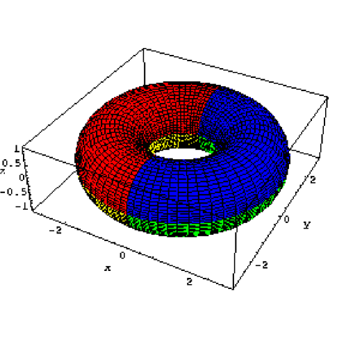
Figure 12: A torus

On the other hand, the method applied to a rectangular net of bidegree $\langle 2,2\rangle$ for an ellipsoid yields base points. For example, it can be shown that a control net of bidegree $\langle 2,2\rangle$ w.r.t. $(-1,1)\times(-1,1)$ for an ellipsoid is given by:

recelnet3 =  {{-8/3, -2, 2/3, 3}, {-8, 0, -2, 1}, {-8/3, 2, 2/3, 3},
   {0, -6, -2, 1}, {0, 0, 6, -1}, {0, 6, -2, 1},
   {8/3, -2, 2/3, 3}, {8, 0, -2, 1},  {8/3, 2, 2/3, 3}}

Unfortunately, the patch corresponding to $F_{3}$ has a base point. The same thing happens for the Steiner roman surface. This is not surprising since neither the sphere nor the real projective plane are of the same topological type as the torus. It can be shown that a control net of bidegree $\langle 2,2\rangle$ w.r.t. $(-1,1)\times(-1,1)$ for the Steiner roman surface is given by:

sqstein3 = {{-2/3, -2/3, 2/3, 3}, {0, -2, 0, 1}, {2/3, -2/3, -2/3, 3},
   {-2, 0, 0, 1}, {0, 0, 0, -1}, {2, 0, 0, 1},
   {-2/3, 2/3, -2/3, 3}, {0, 2, 0, 1}, {2/3, 2/3, 2/3, 3}};

Again, the the patch corresponding to $F_{3}$ has base points.

Another method for drawing rectangular rational surfaces was investigated by DeRose [5] who credits Patterson [16] for the original idea behind the method. Basically, the method consists in using the homogeneous Bernstein polynomials $\binom{p}{i}\binom{q}{j}\,u^{i}t_{1}^{p-i}v^{j}t_{2}^{q-j}$, and to view a rectangular rational surface as a rational map from $\mathbb{RP}^{1}\times\mathbb{RP}^{1}$. Then, by using any $2D$ model of the projective line, it is possible to draw a whole rational surface in one piece.

In general, it is not easy to remove base points. This involves a technique from algebraic geometry known as “blowing-up” (see Fulton [10] or Harris [13]). In the next section, we will present a method for resolving base points in the case of triangular rational surfaces. However, we have not worked out the resolution of base points in the case of rectangular rational surfaces. We leave this problem as an interesting challenge to the reader.

6 Resolving Base Points

We now consider the case in which $F_{\varphi}$ and $F_{\psi}$ (as defined in Section 3) have base points. An example for which this happens is the torus.

Example 3. An elliptic torus can be defined parametrically as follows:

$$\openup 3.0pt\halign to=0.0pt{\hfil$\displaystyle{#}$&$\displaystyle{{}#}$\hfil&\llap{$#$}\cr x &= (a - b\>\sin\varphi)\cos\theta,\cr y &= (a - b\>\sin\varphi)\sin\theta,\cr z &= c\>\cos\varphi.\cr}$$

As usual, we obtain a rational parameterization by expressing $\cos t$ and $\sin t$ in terms of $\tan(t/2)$, and we get the fractions

$$\openup 3.0pt\halign to=0.0pt{\hfil$\displaystyle{#}$&$\displaystyle{{}#}$\hfil&\llap{$#$}\cr x &= \frac{(1 - u^{2})(a(1 + v^{2}) - 2bv)}{(1 + u^{2})(1 + v^{2})},\cr y &= \frac{2u(a(1 + v^{2}) - 2bv)}{(1 + u^{2})(1 + v^{2})},\cr z &= \frac{c(1 - v^{2})}{1 + v^{2}}.\cr}$$

Thus, the torus as a rational surface $F$ is defined by

$$\openup 3.0pt\halign to=0.0pt{\hfil$\displaystyle{#}$&$\displaystyle{{}#}$\hfil&\llap{$#$}\cr x(u, v) &= (1 - u^{2})(a(1 + v^{2}) - 2bv),\cr y(u, v) &= 2u(a(1 + v^{2}) - 2bv),\cr z(u, v) &= c(1 + u^{2})(1 - v^{2}),\cr w(u, v) &= (1 + u^{2})(1 + v^{2}).\cr}$$

Rendering $F$ over $[-1,1]\times[-1,1]$ yields one fourth of the torus, specifically, the front half of the upper half. Performing the change of variables

$$(u,v)\mapsto\biggl{(}\frac{v}{u},\frac{1}{u}\biggr{)},$$

the rational surface $F_{\varphi}$ is defined by

$$\openup 3.0pt\halign to=0.0pt{\hfil$\displaystyle{#}$&$\displaystyle{{}#}$\hfil&\llap{$#$}\cr x(u, v) &= (u^{2} - v^{2})(a(1 + u^{2}) - 2bu),\cr y(u, v) &= 2uv(a(1 + u^{2}) - 2bu),\cr z(u, v) &= c(u^{2} - 1)(u^{2} + v^{2}),\cr w(u, v) &= (u^{2} + v^{2})(u^{2} + 1).\cr}$$

Unfortunately, $x(0,0)=y(0,0)=z(0,0)=w(0,0)=0$, and $(0,0)$ is a base point of $F_{\varphi}$.

Performing the change of variables

$$(u,v)\mapsto\biggl{(}\frac{1}{v},\frac{u}{v}\biggr{)},$$

the rational surface $F_{\psi}$ is defined by

$$\openup 3.0pt\halign to=0.0pt{\hfil$\displaystyle{#}$&$\displaystyle{{}#}$\hfil&\llap{$#$}\cr x(u, v) &= (v^{2} - 1)(a(u^{2} + v^{2}) - 2buv),\cr y(u, v) &= 2v(a(u^{2} + v^{2}) - 2buv),\cr z(u, v) &= c(v^{2} - u^{2})(v^{2} + 1),\cr w(u, v) &= (u^{2} + v^{2})(v^{2} + 1).\cr}$$

Unfortunately, we also have $x(0,0)=y(0,0)=z(0,0)=w(0,0)=0$, and $(0,0)$ is a base point of $F_{\psi}$.

If we try to render the rational surfaces $F_{\varphi}$ and $F_{\psi}$ over $[-1,1]\times[-1,1]$, we discover that some regions of these surfaces are not drawn properly. In these regions, there are holes and many lines segments shooting in all directions! The problem is that $(0,0)$ is a discontinuity point for both surfaces, and that the limit reached when $u$ and $v$ approach $0$ depends very much on the ratio $v/u$. One way to understand what happens is to let $v=ku$, simplify the fractions, and see what is the limit when $u$ approaches $0$. For $F_{\varphi}$, after calculations, we find that the limit when $u$ approaches $0$ is

$$\biggl{(}\frac{a(1-k^{2})}{1+k^{2}},\>\frac{2ak}{1+k^{2}},\>-c\biggr{)},$$

which corresponds to the circle of radius $a$ in the plane $z=-c$. For $F_{\psi}$, after calculations, we find that the limit when $u$ approaches $0$ is

$$\biggl{(}-a+\frac{2bk}{1+k^{2}},\>0,\>-\frac{c(1-k^{2})}{1+k^{2}}\biggr{)},$$

which corresponds to an ellipse in the plane $y=0$, centered at the point $(-a,0,0)$. It is indeed in the neighborhood of these two curves on the torus that $F_{\varphi}$ and $F_{\psi}$ are not drawn properly.

We now propose a method to resolve the singularities caused by base points. The method is inspired by a technique in algebraic geometry known as “blowing-up” (see Fulton [10] or Harris [13]). What is new is that we give formulae for computing “resolved” control nets.

In most cases, base points occur during a subdivision step in which a triangular net with a corner of zeros appears. Using a change of base triangle if necessary, it can be assumed without loss of generality that the corner of zeros has $t$ as one of its vertices. If we display control nets (in $\widehat{{\cal E}}$) with $F(r)$ at the top corner, $F(s)$ as the rightmost lower corner, and $F(t)$ as the leftmost lower corner, a control net $\theta=(\theta_{i,\,j,\,k})_{(i,j,k)\in\Delta_{m}}$ of degree $m$ has the following shape:

$$\openup 3.0pt\halign{\hbox to\displaywidth{$\displaystyle#$}\cr 0.0pt{$\displaystyle\hfill\times\hfill\cr 0.0pt{$\displaystyle\hfill\times\times\hfill\cr 0.0pt{$\displaystyle\hfill\ldots\hfill\cr 0.0pt{$\displaystyle\hfill\times\>\times\>\ldots\times\>\>\times\hfill\cr 0.0pt{$\displaystyle\hfill\overrightarrow{0}\>\times\>\times\>\ldots\times\>\>\times\hfill\cr 0.0pt{$\displaystyle\hfill\overrightarrow{0}\>\>\overrightarrow{0}\>\times\>\times\>\ldots\times\>\>\times\hfill\cr 0.0pt{$\displaystyle\hfill\ldots\hfill\cr 0.0pt{$\displaystyle\hfill\overrightarrow{0}\>\ldots\>\overrightarrow{0}\>\times\>\times\>\ldots\times\>\>\times\hfill\cr 0.0pt{$\displaystyle\hfill\underbrace{\overrightarrow{0}\>\overrightarrow{0}\>\ldots\>\overrightarrow{0}\>\overrightarrow{0}}_{m}\>\underbrace{\times\>\times\>\ldots\times\>\>\times}_{m+1-m}\hfill\cr}}}}}}}}}}$$

It is assumed that all entries designated as $\times$ are nonzero. The more general case can be treated, but it is computationally too expensive to be practical.

Given an affine frame $\Delta rst$ in the plane, recall that a rational surface $F$ of degree $m$ defined by the control net $\theta=(\theta_{i,\,j,\,k})_{(i,j,k)\in\Delta_{m}}$ is the projection onto $\widetilde{{\cal E}}$ of the polynomial surface $G$ in $\widehat{{\cal E}}$ defined by $\theta$. Also, we have

$$G(u,v)=\sum_{i+j+k=m}\theta_{i,\,j,\,k}\,\frac{m!}{i!j!k!}\,u^{i}v^{j}(1-u-v)^{k},$$

for all $u,v\in\mathbb{R}$. It will be convenient to assume that if $\theta_{i,\,j,\,k}\in\widehat{{\cal E}}$ is a weighted point, then its weight is denoted as $w_{i,j,k}$, and if $\theta_{i,\,j,\,k}$ is a control vector, then we assign it the weight $w_{i,j,k}=0$. If we define $w(u,v)$ as

$$w(u,v)=\sum_{i+j+k=m}w_{i,j,k}\,\frac{m!}{i!j!k!}\,u^{i}v^{j}(1-u-v)^{k},$$

whenever $w(u,v)\not=0$, we have

$$F(u,v)=\sum_{i+j+k=m}\theta_{i,\,j,\,k}\,\frac{m!}{i!j!k!}\,\frac{u^{i}v^{j}(1-u-v)^{k}}{w(u,v)},$$

for all $u,v\in\mathbb{R}$.

The “blowing-up” method used here relies on the following observation based on an idea of Warren [18]. Given the polynomial surface $G$ in ${\cal E}$ (and $w$), we define the polynomial surface $G_{b}$ and $w_{b}$ as follows:

$$\openup 3.0pt\halign to=0.0pt{\hfil$\displaystyle{#}$&$\displaystyle{{}#}$\hfil&\llap{$#$}\cr G_{b}(\alpha, \beta) &= G(\alpha(1 - \beta), \alpha\beta),\cr w_{b}(\alpha, \beta) &= w(\alpha(1 - \beta), \alpha\beta).\cr}$$

Since $\alpha(1-\beta)+\alpha\beta=\alpha$, we get

$$G_{b}(\alpha,\beta)=\sum_{i+j+k=m}\theta_{i,\,j,\,k}\,\frac{m!}{i!j!k!}\,\alpha^{i+j}(1-\alpha)^{k}\beta^{j}(1-\beta)^{i},$$

and

$$w_{b}(\alpha,\beta)=\sum_{i+j+k=m}w_{i,j,k}\,\frac{m!}{i!j!k!}\,\alpha^{i+j}(1-\alpha)^{k}\beta^{j}(1-\beta)^{i}.$$

Now, if $\theta_{i,\,j,\,k}=\overrightarrow{0}$ for $i+j<m$ (with $i+j+k=m$), we note that both $G_{b}(\alpha,\beta)$ and $w_{b}(\alpha,\beta)$ are divisible by $\alpha^{m}$. If we define the polynomial surface $\widetilde{G}$ (and $\widetilde{w}$), such that

$$\widetilde{G}(\alpha,\beta)=\frac{G_{b}(\alpha,\beta)}{\alpha^{m}}$$

and

$$\widetilde{w}(\alpha,\beta)=\frac{w_{b}(\alpha,\beta)}{\alpha^{m}},$$

then we have

$$\frac{G_{b}(\alpha,\beta)}{w_{b}(\alpha,\beta)}=\frac{\widetilde{G}(\alpha,\beta)}{\widetilde{w}(\alpha,\beta)},$$

for all $\alpha\not=0$. Furthermore when $\alpha=0$, we have

$$\widetilde{G}(0,\beta)=\sum_{i+j=m}\theta_{i,\,j,\,m-m}\,\frac{m!}{i!j!(m-m)!}\,\beta^{j}(1-\beta)^{i},$$

and

$$\widetilde{w}(0,\beta)=\sum_{i+j=m}w_{i,j,m-m}\,\frac{m!}{i!j!(m-m)!}\,\beta^{j}(1-\beta)^{i}.$$

Thus, for all $\beta$ for which $\widetilde{G}(0,\beta)$ and $\widetilde{w}(0,\beta)$ are not simultaneously null,

$$\frac{\widetilde{G}(0,\beta)}{\widetilde{w}(0,\beta)}$$

is defined, and the polynomial surface $\widetilde{G}$ defines the rational surface $\widetilde{F}$ such that

$$\widetilde{F}(\alpha,\beta)=\frac{\widetilde{G}(\alpha,\beta)}{\widetilde{w}(\alpha,\beta)}.$$

Thus, what happens is that the triangular patch $F$ over $\Delta rst$ is really a four-sided patch, the point $F(t)$ being “blown up” into the rational curve of degree $n$ whose control points are

$$(\theta_{i,\,j,\,m-m})_{i+j=m}.$$

If this rational curve has no base points, then the rational surface patch $\widetilde{F}$ defined by the polynomial surface $\widetilde{G}$ has no base point, and it extends the surface patch $F$ over $\Delta rst$. If it has base points, they are common zeros of some polynomials in $\beta$, and by simplifying by common factors and using continuity, we could eliminate these base points. For simplicity, we will assume that the boundary curve has no base points.

Viewing $\widetilde{G}$ as a bipolynomial surface, note that $\widetilde{G}$ has bidegree $\langle m-m,m\rangle$. Also observe that the function

$$(\alpha,\beta)\mapsto(\alpha(1-\beta),\alpha\beta)$$

maps the unit square with vertices

$$(0,0),(0,1),(1,1),(1,0)$$

onto the triangle $\Delta rst=((0,1),(1,0),(0,0))$, in such a way that the edge $((0,0),(0,1))$ is mapped onto $t$, the vertex $(1,1)$ is mapped onto $s$, and the vertex $(1,0)$ is mapped onto $r$. Furthermore, if $u=\alpha(1-\beta)$ and $v=\alpha\beta$, we get

$$\alpha=u+v$$

and

$$\beta=\frac{v}{u+v}$$

and thus, the map is invertible except on the line $u+v=0$. Thus, we can think of the inverse map as “blowing up” the affine frame $\Delta rst$ into the unit square. Specifically, the point $t$ is “blown up” into the edge $((0,0),(0,1))$.

Figure 13: Blowing up a triangle into a square

The only remaining problem is that the above method yields a rational square patch not given by a control net, and that we often need to map the unit square to an arbitrary base triangle. The second problem is easily solved. Assume that the affine frame $\Delta rst$ has coordinates $((r_{1},r_{2}),(s_{1},s_{2}),(t_{1},t_{2}))$. It is easily seen that the map defined such that

$$\openup 3.0pt\halign to=0.0pt{\hfil$\displaystyle{#}$&$\displaystyle{{}#}$\hfil&\llap{$#$}\cr u &= (s_{1} - r_{1})\alpha\beta+ (r_{1} - t_{1})\beta+ t_{1},\cr v &= (s_{2} - r_{2})\alpha\beta+ (r_{2} - t_{2})\beta+ t_{2},\cr}$$

maps the unit square to the triangle $\Delta rst$, in such a way that the edge $((0,0),(0,1))$ is mapped onto $t$, the vertex $(1,1)$ is mapped onto $s$, and the vertex $(1,0)$ is mapped onto $r$. Some simple calculations show that

$$\openup 3.0pt\halign to=0.0pt{\hfil$\displaystyle{#}$&$\displaystyle{{}#}$\hfil&\llap{$#$}\cr\alpha&= \frac{(s_{2} - r_{2})(u - t_{1}) - (s_{1} - r_{1})(v - t_{2})}{(r_{1} - t_{1})(s_{2} -r_{2}) - (r_{2} - t_{2})(s_{1} - r_{1})},\cr\beta&= \frac{(r_{1} - t_{1})(v - t_{2}) - (r_{2} - t_{2})(u - t_{1})}{(s_{2} - r_{2})(u - t_{1}) - (s_{1} - r_{1})(v - t_{2})},\cr}$$

and thus, the map is only invertible outside the line of equation

$$(s_{2}-r_{2})(u-t_{1})-(s_{1}-r_{1})(v-t_{2})=0,$$

the parallel to the vector $(s_{1}-r_{1},s_{2}-r_{2})$ through $t$.

Now, if $g\colon({\cal P})^{m}\rightarrow\widehat{{\cal E}}$ is the polar form associated with $G$, we can compute the polar form $g_{b}\colon({\cal P})^{m}\times({\cal P})^{m}\rightarrow\widehat{{\cal E}}$ associated with the bipolynomial surface $G_{b}$ as follows:

$$g_{b}(u_{1},\ldots,u_{m},v_{1},\ldots,v_{m})=\frac{1}{m!}\>\sum_{\sigma\in{\cal S}_{m}}g((u_{1}(1-v_{\sigma(1)}),u_{1}v_{\sigma(1)}),\ldots,(u_{m}(1-v_{\sigma(m)}),u_{m}v_{\sigma(m)})),$$

where ${\cal S}_{m}$ denotes the group of permutations on $\{1,\ldots,m\}$. The above formula corresponds to the case of the simple mapping $u=\alpha(1-\beta)$, $v=\alpha\beta$, and it is obvious how to adapt it to the more general map

$$\openup 3.0pt\halign to=0.0pt{\hfil$\displaystyle{#}$&$\displaystyle{{}#}$\hfil&\llap{$#$}\cr u &= (s_{1} - r_{1})\alpha\beta+ (r_{1} - t_{1})\beta+ t_{1},\cr v &= (s_{2} - r_{2})\alpha\beta+ (r_{2} - t_{2})\beta+ t_{2},\cr}$$

Now, over the affine basis $(0,1)$, the square control net $\theta{\mathchoice{\vbox{\hrule height=0.6pt\hbox{\vrule width=0.6pt,height=7.0pt\kern 7.0pt\vrule width=0.6pt} \hrule height=0.6pt}}{\vbox{\hrule height=0.6pt\hbox{\vrule width=0.6pt,height=7.0pt\kern 7.0pt\vrule width=0.6pt} \hrule height=0.6pt}}{\vbox{\hrule height=0.3pt\hbox{\vrule width=0.3pt,height=2.1pt\kern 2.1pt\vrule width=0.3pt} \hrule height=0.3pt}}{\vbox{\hrule height=0.3pt\hbox{\vrule width=0.3pt,height=1.5pt\kern 1.5pt\vrule width=0.3pt} \hrule height=0.3pt}}}=(\theta{\mathchoice{\vbox{\hrule height=0.6pt\hbox{\vrule width=0.6pt,height=7.0pt\kern 7.0pt\vrule width=0.6pt} \hrule height=0.6pt}}{\vbox{\hrule height=0.6pt\hbox{\vrule width=0.6pt,height=7.0pt\kern 7.0pt\vrule width=0.6pt} \hrule height=0.6pt}}{\vbox{\hrule height=0.3pt\hbox{\vrule width=0.3pt,height=2.1pt\kern 2.1pt\vrule width=0.3pt} \hrule height=0.3pt}}{\vbox{\hrule height=0.3pt\hbox{\vrule width=0.3pt,height=1.5pt\kern 1.5pt\vrule width=0.3pt} \hrule height=0.3pt}}}_{i,j})_{0\leq i,j\leq m}$ associated with $g_{b}$ is defined such that

$$\theta{\mathchoice{\vbox{\hrule height=0.6pt\hbox{\vrule width=0.6pt,height=7.0pt\kern 7.0pt\vrule width=0.6pt} \hrule height=0.6pt}}{\vbox{\hrule height=0.6pt\hbox{\vrule width=0.6pt,height=7.0pt\kern 7.0pt\vrule width=0.6pt} \hrule height=0.6pt}}{\vbox{\hrule height=0.3pt\hbox{\vrule width=0.3pt,height=2.1pt\kern 2.1pt\vrule width=0.3pt} \hrule height=0.3pt}}{\vbox{\hrule height=0.3pt\hbox{\vrule width=0.3pt,height=1.5pt\kern 1.5pt\vrule width=0.3pt} \hrule height=0.3pt}}}_{i,j}=g_{b}(\underbrace{0,\ldots,0}_{m-i},\underbrace{1,\ldots,1}_{i},\underbrace{0,\ldots,0}_{m-j},\underbrace{1,\ldots,1}_{j}).$$

However, if $\theta_{i,\,j,\,k}=0$ for $i+j<m$, with $i+j+k=m$, then $\theta{\mathchoice{\vbox{\hrule height=0.6pt\hbox{\vrule width=0.6pt,height=7.0pt\kern 7.0pt\vrule width=0.6pt} \hrule height=0.6pt}}{\vbox{\hrule height=0.6pt\hbox{\vrule width=0.6pt,height=7.0pt\kern 7.0pt\vrule width=0.6pt} \hrule height=0.6pt}}{\vbox{\hrule height=0.3pt\hbox{\vrule width=0.3pt,height=2.1pt\kern 2.1pt\vrule width=0.3pt} \hrule height=0.3pt}}{\vbox{\hrule height=0.3pt\hbox{\vrule width=0.3pt,height=1.5pt\kern 1.5pt\vrule width=0.3pt} \hrule height=0.3pt}}}_{i,j}=0$ for $i<m$, and thus we obtain the rectangular net $\widetilde{\theta}{\mathchoice{\vbox{\hrule height=0.6pt\hbox{\vrule width=0.6pt,height=7.0pt\kern 7.0pt\vrule width=0.6pt} \hrule height=0.6pt}}{\vbox{\hrule height=0.6pt\hbox{\vrule width=0.6pt,height=7.0pt\kern 7.0pt\vrule width=0.6pt} \hrule height=0.6pt}}{\vbox{\hrule height=0.3pt\hbox{\vrule width=0.3pt,height=2.1pt\kern 2.1pt\vrule width=0.3pt} \hrule height=0.3pt}}{\vbox{\hrule height=0.3pt\hbox{\vrule width=0.3pt,height=1.5pt\kern 1.5pt\vrule width=0.3pt} \hrule height=0.3pt}}}$ of degree $(m-m,m)$ associated with $\widetilde{g}$, given by

$$\widetilde{\theta}{\mathchoice{\vbox{\hrule height=0.6pt\hbox{\vrule width=0.6pt,height=7.0pt\kern 7.0pt\vrule width=0.6pt} \hrule height=0.6pt}}{\vbox{\hrule height=0.6pt\hbox{\vrule width=0.6pt,height=7.0pt\kern 7.0pt\vrule width=0.6pt} \hrule height=0.6pt}}{\vbox{\hrule height=0.3pt\hbox{\vrule width=0.3pt,height=2.1pt\kern 2.1pt\vrule width=0.3pt} \hrule height=0.3pt}}{\vbox{\hrule height=0.3pt\hbox{\vrule width=0.3pt,height=1.5pt\kern 1.5pt\vrule width=0.3pt} \hrule height=0.3pt}}}=(\theta{\mathchoice{\vbox{\hrule height=0.6pt\hbox{\vrule width=0.6pt,height=7.0pt\kern 7.0pt\vrule width=0.6pt} \hrule height=0.6pt}}{\vbox{\hrule height=0.6pt\hbox{\vrule width=0.6pt,height=7.0pt\kern 7.0pt\vrule width=0.6pt} \hrule height=0.6pt}}{\vbox{\hrule height=0.3pt\hbox{\vrule width=0.3pt,height=2.1pt\kern 2.1pt\vrule width=0.3pt} \hrule height=0.3pt}}{\vbox{\hrule height=0.3pt\hbox{\vrule width=0.3pt,height=1.5pt\kern 1.5pt\vrule width=0.3pt} \hrule height=0.3pt}}}_{i,j})_{m\leq i\leq m,\,0\leq j\leq m},$$

which corresponds to the rational surface defined by $\widetilde{G}$.

Thus, we know how to compute a rectangular net for the blown-up version $\widetilde{G}$ of $G$. A triangular net of degree $2m-m$ can easily be obtained. Indeed, there is a simple way for converting the polar form $g\colon({\cal P})^{p}\times({\cal P})^{q}\rightarrow\widehat{{\cal E}}$ of a bipolynomial surface of degree $(p,q)$ into a symmetric multilinear polar form $g_{\Delta}\colon({\cal P})^{p+q}\rightarrow\widehat{{\cal E}}$, using the following formula: letting $m=p+q$, we have

$$g_{\Delta}((u_{1},v_{1}),\ldots,(u_{m},v_{m}))=\frac{1}{\binom{m}{p}}\sum_{\begin{subarray}{c}I\cup J=\{1,\ldots,m\}\\ I\cap J=\emptyset\\ |I|=p,\,|J|=q\end{subarray}}g(\prod_{i\in I}u_{i},\prod_{j\in J}v_{j}),$$

where

$$g(\prod_{i\in I}u_{i},\prod_{j\in J}v_{j})=g(u_{i_{1}},\ldots,u_{i_{p}},v_{j_{1}},\ldots,v_{j_{q}}),$$

with $I=\{i_{1},\ldots,i_{p}\}$, and $J=\{j_{1},\ldots,j_{q}\}$.

Note that it is also possible to convert the polar form $f_{\Delta}\colon({\cal P})^{m}\rightarrow\widehat{{\cal E}}$ of a surface of degree $m$ into a symmetric $(m,m)$-multilinear polar form $g\colon({\cal P})^{m}\times({\cal P})^{m}\rightarrow\widehat{{\cal E}}$, using the following formula:

$$g(u_{1},\ldots,u_{m},v_{1},\ldots,v_{m})=\frac{1}{m!}\sum_{\sigma\in{\cal S}_{m}}f((u_{1},v_{\sigma(1)}),\ldots,(u_{m},v_{\sigma(m)})),$$

where ${\cal S}_{m}$ denotes the group of permutations on $\{1,\ldots,m\}$.

Thus, we have a method for blowing up a control net $\theta$ of degree $m$ with a corner of zeros of size $m$, into a triangular net $\widetilde{\theta}$ of degree $2m-m$, by first blowing up the triangular net $\theta$ into a rectangular net $\widetilde{\theta}{\mathchoice{\vbox{\hrule height=0.6pt\hbox{\vrule width=0.6pt,height=7.0pt\kern 7.0pt\vrule width=0.6pt} \hrule height=0.6pt}}{\vbox{\hrule height=0.6pt\hbox{\vrule width=0.6pt,height=7.0pt\kern 7.0pt\vrule width=0.6pt} \hrule height=0.6pt}}{\vbox{\hrule height=0.3pt\hbox{\vrule width=0.3pt,height=2.1pt\kern 2.1pt\vrule width=0.3pt} \hrule height=0.3pt}}{\vbox{\hrule height=0.3pt\hbox{\vrule width=0.3pt,height=1.5pt\kern 1.5pt\vrule width=0.3pt} \hrule height=0.3pt}}}$, and then converting $\widetilde{\theta}{\mathchoice{\vbox{\hrule height=0.6pt\hbox{\vrule width=0.6pt,height=7.0pt\kern 7.0pt\vrule width=0.6pt} \hrule height=0.6pt}}{\vbox{\hrule height=0.6pt\hbox{\vrule width=0.6pt,height=7.0pt\kern 7.0pt\vrule width=0.6pt} \hrule height=0.6pt}}{\vbox{\hrule height=0.3pt\hbox{\vrule width=0.3pt,height=2.1pt\kern 2.1pt\vrule width=0.3pt} \hrule height=0.3pt}}{\vbox{\hrule height=0.3pt\hbox{\vrule width=0.3pt,height=1.5pt\kern 1.5pt\vrule width=0.3pt} \hrule height=0.3pt}}}$ into a triangular net $\widetilde{\theta}$.

Again, it is fairly easy to implement the above method in Mathematica (see Gallier [12]). In the interest of brevity, we content ouselves with some examples.

Going back to Example 3 of this section, a torus, it turns out that in subdividing the nets theta1, theta2, rho1, and rho2, degenerate nets with a corner of zeros are encountered. In fact, these corners have two rows of zeros. and thus, the blowing up method yields nets of degree $6$. For example, the net corresponding to theta1 is resolved to a triangular net, which after $3$ iterations of subdivision, yields the following picture:

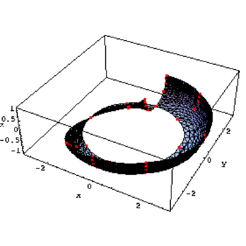
Figure 14: A blow up of patch 3 of a torus

The net corresponding to theta2 is resolved to a triangular net, which after $3$ iterations of subdivision, yields the following picture:

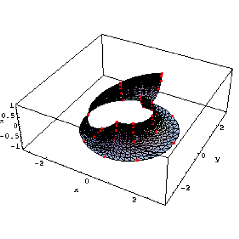
Figure 15: A blow up of patch 4 of a torus

Displaying these two pictures together, we get a shape reminicent of a horse-shoe crab!

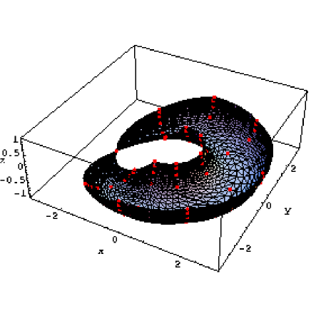
Figure 16: A blow up of patches 4,3 of a torus

Similarly, blowing up the nets rho1 and rho2 yields:

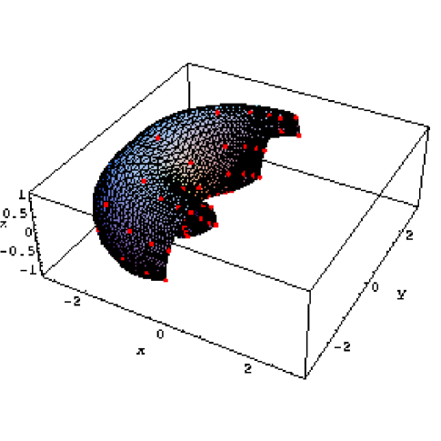
Figure 17: A blow up of patches 5,6 of a torus

Together with the two patches associated with the square $[-1,1]\times[-1,1]$, we get the entire torus. Of course, we could have taken advantage of symmetries, and our point is to illustrate the algorithm.

7 Conclusion

We have presented several methods for drawing whole rational surfaces, defined parametrically or in terms of weighted control points. These methods rely on simple regular subdivisions of the real projective plane or of the torus, and on versions of the de Casteljau algorithm. The main novelty is that the new control nets are obtained very cheaply from the original control net by sign flipping and permutation of indices. One of the advantages of our method is that it is incremental. Indeed, the algorithm produces an approximation of the surface as a sequence of control nets. Thus, if we wish to get better accuracy, we can subdivide each control net in the list. We can also achieve a zooming effect by selectively subdividing some subsequences of control nets. Bajaj and Royappa [2, 3] and DeRose [5] have also investigated methods for drawing whole rational surfaces. However, none of these papers address the problem of computing control nets. A weakness of our method is that it only applies to rational surfaces. On the other hand, although restricted to rational surfaces, our method is efficient, at least when there are no base points. We have also proposed a new method for resolving base points, by computing some refined control nets. Unfortunately, the present version of the method is exponential, and not practical as soon as the degree becomes greater than $4$. Part of the problem is that our method first computes a rectangular control net which is then converted to a triangular net, and this conversion process is exponential. It would be interesting to compute directly a triangular net.

Acknowledgement: We wish to thank Doug de Carlo for some very helpful comments.

References

[1]
Paul Appell.
Traité de Mécanique Rationelle, Tome I: Statique, Dynamique
du Point.
Gauthier-Villars, sixth edition, 1941.
[2]
C. Bajaj and A. Royappa.
Triangulation and display of arbitrary rational parametric surfaces.
In R. Bergeron and A. Kaufman, editors, IEEE Visualization ’94
Conference. IEEE, 1994.
[3]
C. Bajaj and A. Royappa.
Finite representation of real parametric curves and surfaces.
Intl. J. of Computational Geometry and Applications, pages
313–326, 1995.
[5]
Tony D. DeRose.
Rational Bézier curves and surfaces on projective domains.
In G. Farin, editor, NURBS for Curve and Surface Design, pages
35–45. SIAM, Philadelphia, Pa, 1991.
[6]
Gerald Farin.
NURB Curves and Surfaces, from Projective Geometry to practical
use.
AK Peters, first edition, 1995.
[7]
Gerald Farin.
Curves and Surfaces for CAGD.
Academic Press, fourth edition, 1998.
[8]
J.-C. Fiorot and P. Jeannin.
Courbes et Surfaces Rationelles.
RMA 12. Masson, first edition, 1989.
[9]
J.-C. Fiorot and P. Jeannin.
Courbes Splines Rationelles.
RMA 24. Masson, first edition, 1992.
[10]
William Fulton.
Algebraic Curves.
Advanced Book Classics. Addison Wesley, first edition, 1989.
[11]
Jean H. Gallier.
Curves and Surfaces In Geometric Modeling: Theory And
Algorithms.
Morgan Kaufmann, first edition, 1999.
[12]
Jean H. Gallier.
Geometric methods and Applications For Computer Science and
Engineering.
TAM No. 38. Springer–Verlag, first edition, 2000.
[13]
Joe Harris.
Algebraic Geometry, A first course.
GTM No. 133. Springer Verlag, first edition, 1992.
[14]
D. Hilbert and S. Cohn-Vossen.
Geometry and the Imagination.
Chelsea Publishing Co., 1952.
[15]
J. Hoschek and D. Lasser.
Computer Aided Geometric Design.
AK Peters, first edition, 1993.
[16]
R. Patterson.
Projective transformations of the parameter of a rational
Bernstein-Bézier curve.
ACM Transactions on Graphics, 4:276–290, 1986.
[17]
Lyle Ramshaw.
Blossoming: A connect-the-dots approach to splines.
Technical report, Digital SRC, Palo Alto, CA 94301, 1987.
Report No. 19.
[18]
J. Warren.
Creating multisided rational Bézier surfaces using base points.
ACM Transactions on Graphics, 11(2):127–139, 1992.