Threshold-Controlled Global Cascading in Wireless Sensor Networks

Abstract

We investigate cascade dynamics in threshold-controlled (multiplex) propagation on random geometric networks. We find that such local dynamics can serve as an efficient, robust, and reliable prototypical activation protocol in sensor networks in responding to various alarm scenarios. We also consider the same dynamics on a modified network by adding a few long-range communication links, resulting in a small-world network. We find that such construction can further enhance and optimize the speed of the network’s response, while keeping energy consumption at a manageable level.

I Introduction

Many of the modern and important technological, information and infrastructure systems can be viewed as complex networks with a large number of components [1, 2, 3]. The network consists of nodes (or agents) and (physical or logical) links connecting the nodes. These links facilitate some form of interaction or dynamics between the nodes. Spreading information fast across such networks with efficient and autonomous control is a challenging task. Wireless Sensor Networks (WSNs) provide an example where understanding dynamical processes on the network is crucial to develop efficient protocols for autonomous operation.

A sensor network is comprised of a large number of sensor nodes which monitor, sense, and collect data from a target domain and then process and transmit the information to the specific sites (e.g., headquarters, disaster control centers). There are many potential applications of sensor networks including military, environment and health areas (for a taxonomy of sensors networks see [4]). There are fundamental differences between a sensor network and other wireless ad-hoc networks. First, sensor nodes are often densely deployed (typically 20 sensor per cubic meter) [5] so that the underlying network has high redundancy for sensing and communications. Accordingly, the size of sensor networks may be several orders of magnitude larger than the other ad-hoc networks. Hence, scalability of sensor network operations is of utmost importance (see, for example [6] for scalable coordination challenges and solutions or [7] scalable, self-organizing designs for sensor networks and for limits on achievable capacity and delay in mobile wireless networks). Second, sensor nodes have limited battery power without recharging capabilities. Nodes running out of power may cause topology changes in sensor networks even without mobility (see for example  [8] for scalable and fault-tolerant routing and [9] for communal routing in which some of the nodes take over routing for the sleeping neighbors). Third, new sensors with fresh batteries may be injected to a sensor network, already in use, to enhance and ensure its correct operation. Finally, the sensor nodes may be deployed in adversarial environments such as battlefields, hostile territories or hazardous domains that make their management, control and security very difficult. Combined with diverse environments, ranging from deserts to rain forests, from urban areas to battlefields and habitats of protected species [10], these challenges make designing sensor networks that can operate reliably and autonomously (totally unattended) very difficult.

The focus of this paper is on outliers detection in wireless sensor network but the challenge is the same as in the above mentioned work, to design scalable, energy efficient algorithms for communication and coordination. Outlier detection is an essential step which precedes most any analysis of data. It is used either with the intention of suppressing the outliers or amplifying them. The first usage (also known as data cleansing) is important when the analysis carried on the data is not robust. Examples for such applications are optimization tasks, including routing (where erroneous data may lead to infinite loops). The second usage is important when looking for rare patterns. This often happens in adversarial domains such as battlefield monitoring, controlling a boundary or a perimeter of protected objects or intrusion detection.

Outliers are caused not only by external factors, but also by imperfections in the acquisition of the data. They typify error prone systems, specifically those which ought to operate in harsh environmental conditions and make imperfect measurements of external phenomena. Another setting in which outliers may occur is whenever an adversary can control the measurement (but not the computation and communication) of a device. In this setting, outliers detection can either detect the manipulation of the data, or limit the extent to which the data is manipulated. Thus, in some settings, outliers detection limits the ability of an adversary to divert the result.

Several factors make WSNs especially prone to difficulties in outliers detection. First, WSNs collect their data from the real world using imperfect sensing devices. Next, they are battery operated and thus their performance tend to deteriorate as power is exhausted. Moreover, as sensor networks may include thousands of devices, the chance of error accumulates in them to high levels. Finally, sensors are especially exposed to manipulation by adversaries in their usage for security and military purposes. Hence, it is clear that outlier detection should be an inseparable part of any data processing that takes place in sensor networks. In this paper, we investigate a simple model of cleansing and amplifying outliers in wireless sensor networks. WSN environments pose several restrictions on outliser computation, such as: (i) it has to be done in-network because communication of raw data would deplete batteries, (ii) communication may often be asymmetric, (iii) the data is streaming, or at least dynamically updated, and (iv) both spatial and temporal locality of the data are important for the result – data points sampled by nearby sensors during a short period of time ought to be more similar than ones sampled by far off sensors over a large time interval. Hence, in this paper, we assume that the number of nodes reporting outliers is significant in making a decision to amplify or not the outlier discovery.

Sensor networks are both spatial and random. As a large number of sensor nodes are deployed, e.g., from vehicles or aircrafts, they are essentially scattered randomly across large spatially extended regions. In the corresponding abstract graph two nodes are connected if they mutually fall within each others transmission range, depending on the emitting power, the attenuation function and the required minimum signal to noise ratio. Random geometric graphs (also referred to as Poisson/Boolean spatial graphs), capturing the above scenario, are a common and well established starting point to study the structural properties of sensor network, directly related to coverage, connectivity, and interference. Further, most structural properties of these networks are discussed in the literature in the context of continuum percolation [11, 12, 13].

The common design challenge of these networks is to find the optimal connectivity for the nodes: If the connectivity of the nodes is too low, the coverage is poor and sporadic. If the node connectivity is too high, interference effects will dominate and results in degraded signal reception [14, 15, 16, 17]. From a topological viewpoint, these networks are, hence, designed to “live” somewhat above the percolation threshold. This can be achieved by adjusting the density of sensor nodes and controlling the emitting power of the nodes; various power-control schemes have been studied along these lines [14, 17]. In this paper we consider random geometric graphs above the percolation threshold, as minimal models for the underlying network communication topology. The focus of this work is to study novel cascade-like local communication dynamics on these well studied graphs.

Here, we focus on the scenario where the agents (the individual sensors) are initially in an inactive mode, typically performing some periodic local measurements. However, if an alarm-triggering event is detected locally by a (few) agent(s), the network, as a whole should “wake-up” (all agents turning to an active state), to closely monitor the spatial and temporal behavior of the underlying phenomena that caused the alarm (e.g., spread of a fire or toxic chemicals). This process of turning agents from an inactive state to an active one, requires some kind of local rules between agents. There are three (somewhat conflicting) objectives for constructing an optimal protocol:

1. reliability, so local erroneous events or false-alarms are suppressed and do not result in a “global wake-up”;

2. speed, so that sensors can monitor the underlying physical, chemical, etc. phenomena;

3. energy efficient, so main concern in sensor networks, namely energy limitation is addressed.

To this end, we will consider a simple threshold-based model (or multiplex propagation) [18, 19, 20] on the sensor network with the potential to efficiently facilitate the transition of the nodes from an inactive to an active state. First, we will consider the threshold-based cascade dynamics on random geometric networks. Then we will experiment with the “addition” of a few long-range communication links, representing multi-hop transmissions. In particular, we will investigate the benefits in shortening the global transition time versus the increase in communication (and therefore also energy) costs. Such networks, commonly referred to as small-world networks [21, 22], has long been known to speed up the spread of local information to global scales [1, 2, 3, 21, 22] and to facilitate autonomous synchronization in coupled multi-component systems [23, 24, 25, 26, 27].

II Threshold-Based Propagation on Random Geometric Networks

II-A Random Geometric Networks

As mentioned in the Introduction, in this paper we consider random geometric graphs [11, 12, 13] as the simplest topological structures capturing the essential features of ad hoc sensor networks. $N$ nodes are distributed at uniformly random in an $L\times L$ spatial area. For simplicity we consider identical radio range $R$ for all nodes. Two nodes are connected if they fall within each other’s range. An important parameter in the resulting random geometric graph is the average degree or connectivity $\alpha$ (defined as the average number of neighbors per node $\overline{k}$), $\alpha\equiv\overline{k}=2K/N$, where $K$ is the total number of links and $N$ is the number of nodes. In random geometrical networks, there is a critical value of the average degree, $\alpha_{c}$, above which the largest connected component of the network becomes proportional to the total number of nodes (the emergence of the giant component) [11, 12, 13]. For a given density of nodes $\rho$, there is a direct correspondence between the degree of connectivity $\alpha$ and the radio range $R$ of each node [11, 12, 13],

$$\alpha=\rho\pi R^{2}\;.$$ (1)

In what follows, for convenience, we will use $R$ instead of $\alpha$, as the relevant parameter controlling the connectivity of the network.

II-B Threshold-Controlled Propagation

The phenomenon of large cascades triggered by small initial shocks, originally motivated by propagation in social networks [18], can be described by a simple threshold-based model [18, 19, 20]. This model considers the dynamics on a network of interacting agents (wireless sensors in the present context), each of which must decide between two alternative actions and whose decisions depend explicitly on the actions of their neighbors according to a simple threshold rule. Unlike in simple diffusive propagation, such as the spread of a disease, where a single node is sufficient to “infect” (activate) its neighbors, in threshold-based (multiplex) propagation node activation requires simultaneous exposure to multiple active neighbors. Here, we implemented these simple rules for random geometric networks, capturing the topological features of wireless sensor networks.

The detailed description of the threshold model is as follows. Each agent can be in one of two states: state $0$ or state $1$, corresponding to the agent being inactive or active, respectively. Upon observing the states of its $k$ neighbors, an agent turns its state from 0 to 1 only if the fraction of its active neighbors is equal to or larger than a specific threshold $\varphi$. In this work we are interested in the temporal characteristics of global cascades (network “wake-ups”), hence once a node turns active, it remains active for the duration of the evolution of the system.

We consider a system of $N$ agents located at the nodes of a random geometric network. Each agent is characterized by a fixed threshold $0\leq\varphi\leq 1$. For simplicity all agent have the same threshold. Initially the agents are all off (in state 0). The network is perturbed at time $t=0$ by a small fraction of nodes that are switched on (switched to state 1). The number of active nodes then evolves at successive time steps with all nodes updating their states simultaneously (synchronous updating) or in random, asynchronous order (asynchronous updating) according to the threshold rule above. Once a node has switched on, it remains on (active) for the duration of the experiment.

For sensor networks, we are interested in the behavior of the network under emergent situation which is represented by small perturbation in the initial condition. In our investigation, the focus is on:

1. the probability that a successful global cascade will be ignited by small fraction of initial seed(s);

2. time needed for a global cascade, that is how fast an initial shock will spread out to the entire network; and

3. the energy used for communication between agents in a successful global cascade.

The last quantity is an important factor in designing wireless sensor networks. Here the term cascade refers to an event of any size triggered by initial seed(s), whereas global cascade is reserved for sufficiently large cascades (corresponding to a final fraction of active agents, larger than a cutoff fraction of large, but finite network).

II-C Simulation and Analysis

We simulated systems consisting of $N=10^{4}$ sensor nodes distributed randomly in a $L\times L=10^{3}\times 10^{3}$ (in arbitrary units) two-dimensional region with periodic boundary conditions. These nodes are employed (for simplicity) with identical communication range $R$ to form a random geometric network. For a fixed density of sensor nodes, $\rho=N/L^{2}$, the relationship between the average degree $\alpha$ and the radio range $R$ is given by Eq. (1).

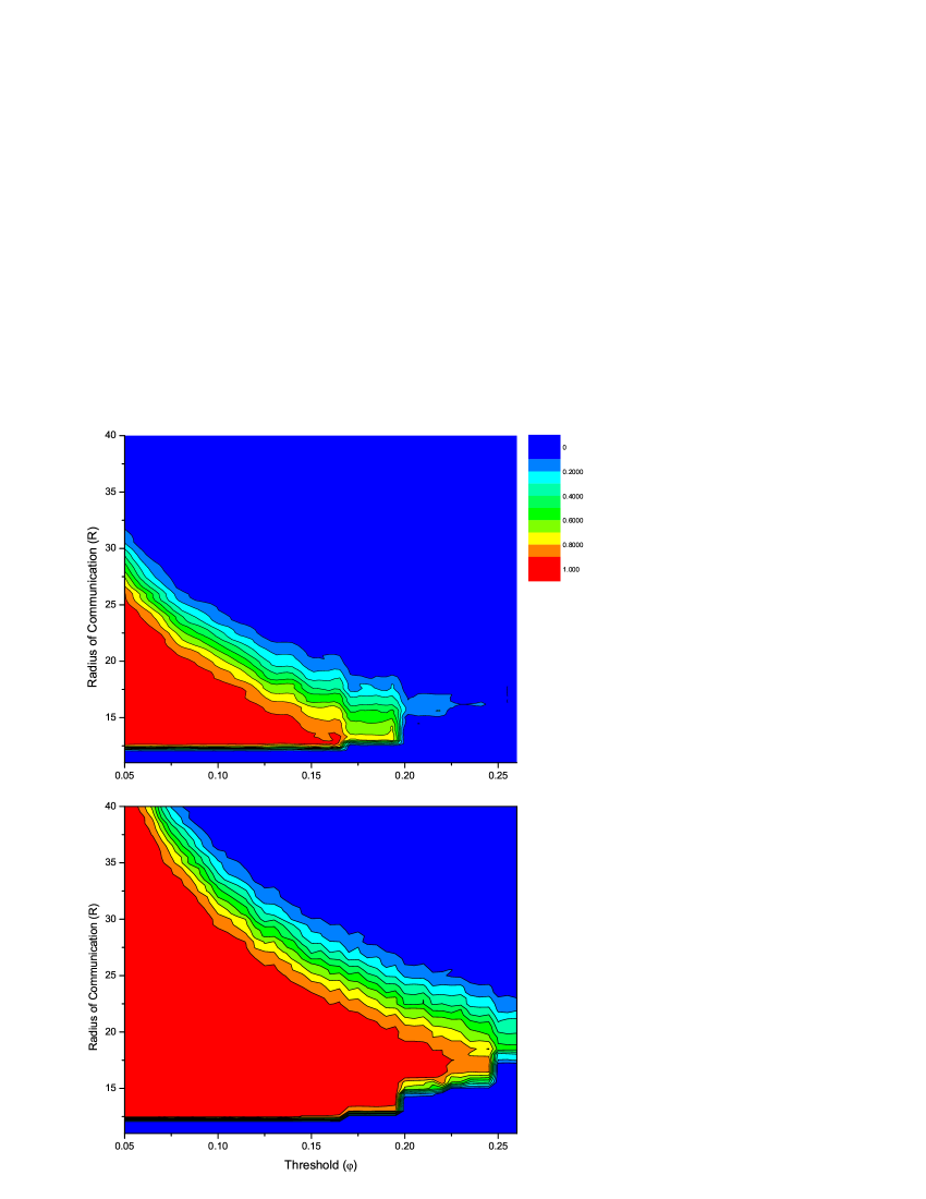
Figure 1: Phase diagram in the plane of threshold and radio range $(\varphi,R)$. The cascade window is enclosed by two different types of boundaries. (a) the cascade window when the size of the initial seed is one. (b) the cascade window when the size of the initial seed is three. Both graphs are obtained at the system size $N=10^{4}$ and averaged over 1,000 simulation runs.

Figure 1 displays the phase diagram for the cascade dynamics on the $(\varphi,R)$ plane in terms of the probability of global cascades for two differentinitial seed size. Each point in the graph is obtained by averaging over $1000$ simulations (including different network topologies and initial cascade seeds). For seed size one, only a single node is activated initially in the network. For seed size three, we randomly select three neighboring (connected) nodes as a seed and turn them active as the initial condition. In the phase diagram, by fixing the threshold $\varphi$ and going along the line parallel to the $R$-axis, hence increasing the radius of communication $R$, the system exhibits two different phase transition as shown in Fig. 2. The first transition occurs at about $R_{c1}\simeq 12.5$ (corresponding to $\alpha\simeq 4.9$) where the probability of global cascades sharply rises from 0 to around 1 for both initial seed sizes. We refer to this phase transition as phase transition I. Further increasing the communication range $R$, the probability of a global cascade slowly drops to 0. This phase transition is referred to as phase transition II. Phase transition I is inherently related to the emergence of the giant component in a random geometrical network [11, 12, 13]. Below the critical value $R_{c1}$, the network is poorly connected, hence no cascade can spread to global scales. Above $R_{c1}$ the giant component can support global cascades, depending on the threshold $\varphi$. This transition across $R_{c1}$ is sharp, related to the scaling properties of the giant component of the random geometric network. For sufficiently small threshold values $\varphi<1/\alpha$ the probability of global cascades is close to 1 in a well connected graph, yielding the upper boundary of the region where global cascades are possible, $R_{c}(\varphi)$. As the range $R$ is increased, while the threshold $\varphi$ is held fixed, nodes will have have so many neighbors that they cannot be activated by a single active agent. Since the relationship between the average degree and the range follows Eq. (1), the approximate location of the boundary associated with phase transition II scales as

$$R_{c}(\varphi)\sim 1/\sqrt{\varphi}\;.$$ (2)

Figure 3 is the snapshots from a successful global cascade with non-periodical boundary condition. At time $t=170$ the fraction of active nodes exceeds 0.85 and completes the global cascade.

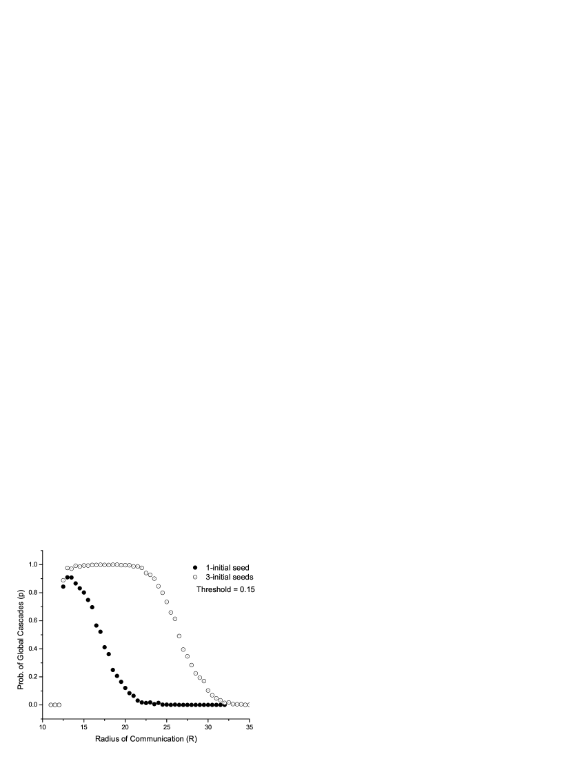
Figure 2: Cross section of cascade window from Fig. 1, at $\varphi=0.15$, with one initial seed node (solid circles) and with three initial seed nodes (open circles). Choosing any value at which these two curves separate sufficiently far away from which other enables the network to suppress the global cascade triggered by poorly supported events. The radius $R$ is connected to the average network degree $\alpha$ according to Eq. (1).

In reality, it is possible that one of the sensors fails or turns active and sends out an alarm message by accident. One of our objectives is to construct local dynamics where global “wake-ups” due to erroneous events or miss-alarms are suppressed or possibly excluded. This should be accomplished in an autonomous fashion, i.e., without any external filtering or intervention. To this end, first, it is reasonable to assume that the probability that a specific node will send out an erroneous alarm is very small. Thus, if, e.g., three neighboring nodes become active simultaneously, it should be considered to be a real event. Comparing Fig. 1(a) (one initial seed node) and Fig. 1(b) (three initial seed nodes), it is clear that to prevent miss-alarms by eliminating global cascades triggered by one initial seed, while allowing them when triggered by the real event defined as above, we should chose the region outside of the global cascades (blue/dark colored region) of Fig. 1(a) but inside the global cascade region (red/light colored region) of Fig. 1(b) by picking proper $R$ and $\varphi$. Fig. 2 is the cross section of phase diagram at $\varphi=0.15$. We can see that if the radius of communication range is within $20<R<25$, the probability of global cascades triggered by three initial seed nodes is still very close to 1 while the probability of global cascades triggered by a single initial seed essentially drops to 0. Hence, by choosing the proper values of $R$ and $\varphi$, according to the phase diagrams, we can prevent miss-alarms and, at the same time, ensure that real events will trigger global cascades with near certainty.

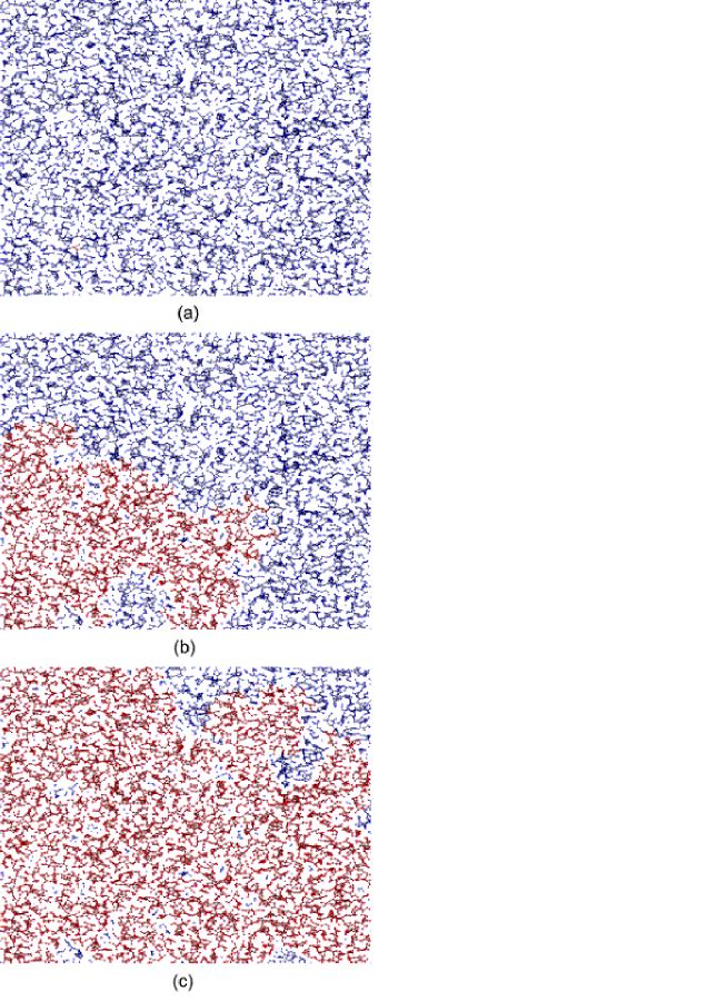
Figure 3: Snapshots of the regular random geometric network evolving with time after the initial shock. Blue dots are in state 0, red ones are in active state. Black lines are local links. Snapshots are taken at time-step (a) t=0; (b) t=80; (c) t=170. The network implemented the synchronous updating with $N=10^{4}$, $\varphi=0.12$, and $R=16.0$.

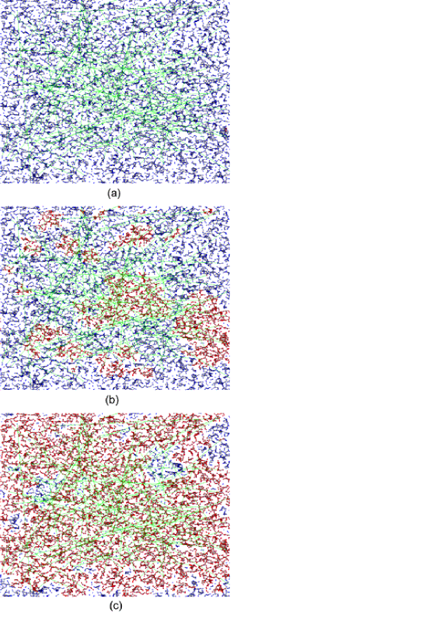
Figure 4: Snapshots of the small-world network evolving with time after the initial shock. Green lines are random long-ranged links. Snapshots are taken at time-step (a) t=0; (b) t=28; (c) t=45. Messages propagate much faster than in regular random geometric networks. The network implemented the synchronous updating with $N=10^{4}$, $\varphi=0.12$, and $R=16.0$.

III Threshold-Model with Small-World Links

ea The small world phenomenon originates from the observation that individuals are often linked by a short chain of acquaintances. Milgram [28] conducted a series of mail delivery experiments and found that an average of “six degrees of separation” exists between senders and receivers. The small-world property (very short average path length between any pair of nodes) were also observed in the context of the Internet and the world wide web. Motivated by social networks [22], and to understand network structures that exhibit low degrees of separation, Watts and Strogatz [21] considered the re-wiring of some fraction of the links on a regular graph, and observed that by re-wiring just a small percentage of the links, the average path length was reduced drastically (approaching that of random graphs), while the clustering remains almost constant (similar to that of regular graphs). This class of graphs was termed small-world graphs to emphasize the importance of random links acting as shortcuts that reduce the average path length in the graph. In the following, we will continue to study random geometric graphs in the context of wireless sensor networks but with the goal of investigating the applicability of the small world concept to these networks. The topological properties (such as the shortest path and the clustering coefficient) of small-world-like sensor networks have been studied in [29]. Here, we focus on the effect of adding some random communication links between possibly distant nodes, on the dynamics on the network.

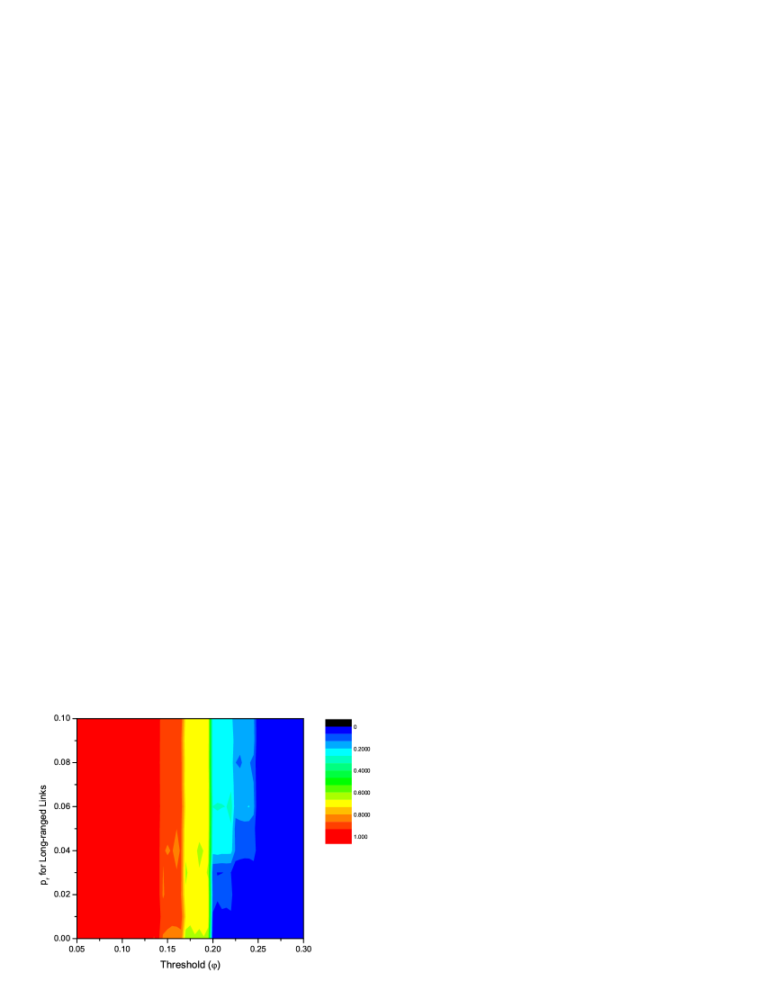
Figure 5: Phase diagram in the plane of threshold and the probability of long-ranged links $(\varphi,p_{r})$. The cascade window is enlarged as we increase the probability of long-ranged links ($p_{r}$). The graph is obtained at the system size $N=10^{4}$ with $R=14$ and averaged over $1,000$ simulations.

As previously, we randomly deploy $N=10^{4}$ sensor nodes in a $L\times L=10^{3}\times 10^{3}$ area, set a fixed radio range $R$ to connect them, and generate the corresponding random geometric network. In addition, we also add random “long-range” links to this backbone to construct a small-world-like network. Random (possibly long-range) connections are constructed by adding a fixed number of random links, so that the total number of random added edges is $p_{r}N$ with $p_{r}\ll 1$. Alternatively, one can construct statistically identical networks by adding a random link emanating from each node with probability $p_{r}$. The procedure has several different realizations, depending on how $p_{r}$ (in the above probabilistic interpretation) varies with the underlying spatial distance between the randomly connected two nodes.

1. $p_{r}=constant$, in which case there are no restrictions on the length of random long range links;

2. $p_{r}\propto 1/d^{\delta}$, where $d$ is the distance between the two chosen nodes and $\delta$ is a parameter;

3. $p_{r}=constant$ for $d\leq d_{c}$ and $p_{r}=0$ for $d>d_{c}$, where $d$ is the distance between the two picked nodes and $d_{c}$ is a parameter to which we refer as cutoff distance.

The dynamics on the network is defined by the same threshold model that was discussed earlier. Here we show results for the case when the size of the initial seed is set to one. Thus, the dynamics is controlled by threshold $\varphi$, the radio range $R$, and the probability of a long-range links $p_{r}$.

The addition of small-world links is expected to speed up propagation (reduce time for global cascades to complete) in the region where global cascades are possible [20]. Focusing on the three quantities outlined earlier, the probability of global cascades (yielding the phase diagram), the average global cascade times, and energy costs, compared to the original random geometrical network are discussed below. The measured observables are averaged over 1,000 simulations. The time needed for global cascades is averaged over all successful global cascades with the same model parameters.

Snapshots of a successful global cascade in the small-world network is shown in Fig. 4. Comparing the snapshots from regular random geometric networks, nodes in small-world networks can be ignited by his neighbors in distance via long-ranged links added to the network, thus expedite the speed of message propagation.

Figure 6: Effect of long-ranged links on the dynamics of random geometric graph under threshold rule. The introduction of long-ranged links decreased the time needed for cascades but increased the energy cost. Symbols mean: $p_{r}=0$ (solid circles); $p_{r}=0.05$ (open circles); $p_{r}=0.01$ (open triangles); $p_{r}=0.02$ (open diamonds). The graph is averaged over $1,000$ simulations with synchronous updating and the threshold fixed at $\varphi=0.12$.

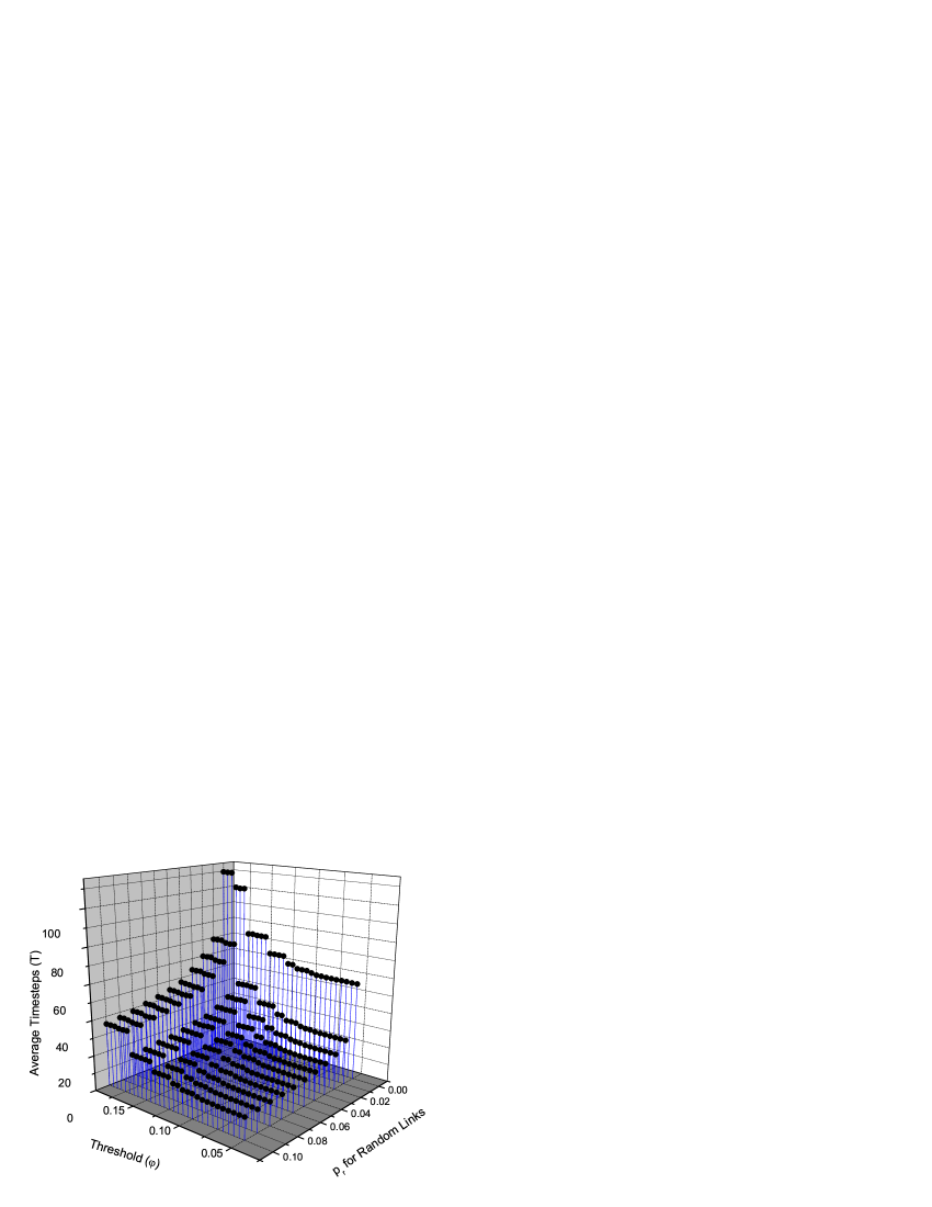
Figure 7: The reduction in global cascade time resulting from the increased number of long-ranged links. Similar behavior as in Fig. 6 is observed when radio range $R$ is fixed. The graph is averaged over 1,000 simulations with synchronous updating, $N=10^{4}$, and $R=14.0$.

Next, we define the energy consumption during a successful global cascade. The total energy consumption in a wireless sensor network is, in most part, due to communication between nodes, computing, and storage (neglecting some smaller miscellaneous costs). The communication is the main part of energy consumption, and is directly related the network structure and dynamics, while energy used for computing can be regarded as a constant, so it can be easily evaluated. Consequently, in the following, we only consider the energy consumption in communications between sensor nodes.

There are two kinds of communication in small-world graphs. First is the local communication. According to the nature of sensor nodes, the wireless broadcast is the most commonly used method for local communication. Thus, the energy cost for local broadcast is proportional to the square of radio range $R$, $E_{l}=cR^{2}$, where $c$ is a coefficient that we scaled to 1. It should also be noted that a message send by a specific node can be received by all his local neighbors, regardless of the number of them, by a single broadcast. The second type of communication is the long-ranged one. The energy cost for long-ranged communication depends on how this communication is implemented, including solutions such as a directional antenna, multi-hop transmission, global flooding, etc. In this paper, we consider multi-hop transmissions in which messages reach their destination following a multi-hop route. The energy cost of such a transmission (for well-connected networks) can be approximated as

$$E_{r}\simeq cR^{2}(\frac{d}{R})=cRd=E_{l}\frac{d}{R},$$ (3)

where $d$ is the distance between two nodes. Unlike in case of broadcast, each pair of nodes that has a long-ranged link between them will incur additional energy to communicate. Hence, the total energy consumption in communication for a successful global cascade with $m$ local communications and $n$ long-ranged communications is:

$$E=mE_{l}+nE_{r}$$ (4)

Since $n=p_{r}N$, then denoting the average length of long-range links as $\overline{d}$ and using an approximation $m\simeq N$ (the exact value of $m$ is equal to the number of nodes participating in the global cascade), the energy cost can be rewritten as:

$$E\simeq cN(R^{2}+p_{r}\overline{d}R)=NE_{l}\left(1+\frac{p_{r}\overline{d}}{R}\right)\;.$$ (5)

The first term corresponds to the local communication energy, while the second term represents the additional energy needed for the long-ranged links. The ratio of the long-ranged link communication energy to the local communication energy is proportional to the probability of long-ranged links $p_{r}$ and the average link length and inversely proportional to the radio radius $R$.

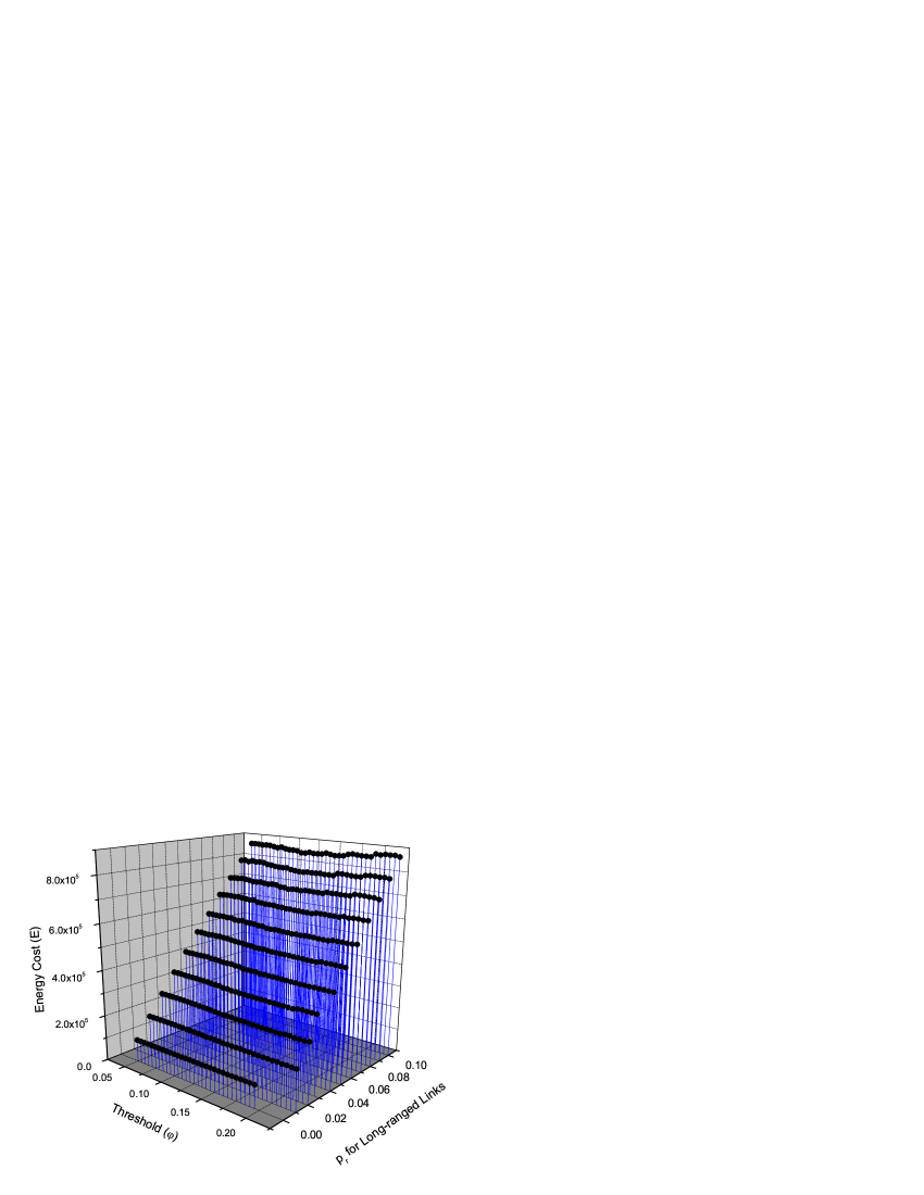
Figure 8: The energy cost of global cascades as a function of the threshold and the density of long-ranged links. The graph is averaged over 1,000 simulations with synchronous updating, $N=10^{4}$, and $R=14.0$.

Figure 9: A comparison of average time and energy costs with different cutoff distance of long-ranged links. Different symbols are, $p_{r}=0$ (solid circles); $p_{r}=0.01$, $d_{c}=\sqrt{2}L$ (open circles); $p_{r}=0.01$, $d_{c}=0.5L$ (open triangles); $p_{r}=0.01$, $d_{c}=0.3L$ (cross). The network implemented the synchronous updating with the threshold fixed at $\varphi=0.12$.

Graphs for the cascade window, after adding the long-ranged links, are similar to that of the model without long-range links [Fig. 1]. The most significant difference is that the lower boundary of the cascade window (which we referred to as phase transition I) shifts downwards by a small amount ($\sim 0.5-1.0$) toward smaller $R$. As we discussed above, a sufficiently large value of $R$ is necessary for the entire graph to be well connected and to be able to support global cascades. By adding long-ranged links, it will be more likely that several small clusters would be connected via these long-ranged links to form a larger cluster, hence lowering the boundary of cascade windows. Figure 5 displays the phase diagram in terms of the probability of global cascades on the plane of the threshold $\varphi$ and the probability of random long range links $p_{r}$, $(\varphi,p_{r})$, when the radio range $R$ is fixed at 14.0. Different from the results of Ref. [20] (as a result of adding as opposed to re-wiring random links), the cascade window somewhat enlarges at a specific region of $(\varphi,R)$ when $p_{r}$ increases.

The advantage of the small-world links is that they can significantly decrease the global cascade time. In other words, alarms and messages propagate faster in small-world graphs than in the original random geometric graphs, as shown in Figs. 6 and 7. For fixed threshold, the time needed for a global cascade decreases monotonously as $R$ increases in regular random geometric graphs. In contrast, in small-world graphs, the average time is much lower and reaches its optimal (minimum) value at $R\simeq 15.0$. The more long-ranged links are added to the network, the lower the average time is. Meanwhile, due to the long-range communications, the average energy cost for a successful global cascade is also increasing, linearly with $p_{r}$, in agreement with Eq. (5) as can be seen in Fig. 8.

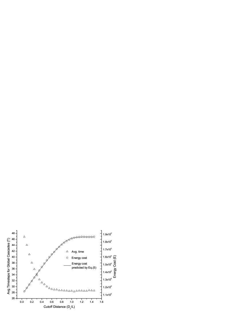
Figure 10: A dependence of the average time and energy costs on the cutoff distance when the threshold and radio range are both fixed. According to the shape of these two curves, we can optimize the system behavior by varying the cutoff distance $d_{c}$. Open triangles are the average time, open circles are the energy cost and solid line is the energy cost predicted by Eq. (5) with $R=16$, $\varphi=0.12$ and synchronous updating.

The above observations can be used to develop a scheme to compensate the increase in energy cost caused by the added long-range links. In the discussion above, the distribution of the distance of the long-range links was uniform. Next, we explore the effects of “suppressing” the occurrence of links with large spatial length. While one can implement, e.g., a power-law or an exponentially-tailed distribution for the spatial length of the added random links, here, for simplicity and to ease technical realizations, we use a sharp cutoff for $p_{r}(d)$,

$$p_{r}(d)=\left\{\begin{array}[]{rl}p_{r0}&\mbox{if $d\leq d_{c}$}\\ 0&\mbox{if $d>d_{c}$},\end{array}\right.$$ (6)

where $d_{c}$ is the cutoff distance for the long-ranged links. This distance may represent the range of a uni-directional antenna of special sensor nodes. Adding a small amount, $p_{r}N$, of such random links to the network will provide the long-range links in the network without the need to implement multi-hop routing.

Scaling $d_{c}$ with the spatial size $L$ of the system, when $d_{c}\geq\sqrt{2}L$, there is no restriction on the long-range link length. The average time and energy costs for global cascade under the restriction of long-range links is shown in Fig. 9.

It can be seen that even putting a strong restriction of the longest link distance ($d_{c}<0.5L$) only slightly increases the average time for successful global cascades. However, under the same restrictions, the energy cost drops significantly, proportionally to the decrease in the average long-ranged link length, as predicted by Eq. (5). In particular, we explored the behavior of the average time ($T$) and the energy cost ($E$) vs. different cutoff distances ($d_{c}$) when $R$ and $\varphi$ are both fixed [Fig. 10]. The average time is close to its minimum when $d_{c}>0.4L$ while the energy cost has still not saturated until $d_{c}>1.0L$. Clearly, one can make a trade-off between the speed of message propagating and the energy cost with different cutoff distances of the long-range links. Depending on various applications and scenarios, we can choose different $d_{c}$ to make the network respond faster to emergencies or be more efficient in terms of energy used.

IV Conclusion

In this paper, we explored cascade dynamics in threshold-controlled (multiplex) propagation on random geometric networks as a simple yet effective model of outliers cleansing and amplifying in wireless sensor networks. Hence, the local dynamics of cascading can serve as an efficient, robust, and reliable basic activation protocol for responding to various alarm scenarios and distinguishing between false (few outliers indicating alarm discovered) and real alarms (several outliers detected in close proximity of each other). We also found that the network modified by adding a few long-range communication links, resulting in a small-world network, changes the speed of the network’s response. Hence, such construction can further enhance and optimize the speed of the network’s response, while keeping energy consumption at a manageable level. More realistic “backbone” topologies (beyond the minimalist random geometric graphs) can be readily constructed and studied, based on the minimum requirements of the local signal-to-noise for signal detection. Future studies will address communication dynamics on such networks.

The presented research raised also several questions that we plan to pursue in future research. One of the most fundamental questions is the impact of synchrony or asynchrony of the alarm propagation. Another is about the technical means of creating the long-range links. Instead using multi-hop transmission, we can foresee mixing a small percentage of nodes with directional antennas among all sensors and using those nodes to support long-range links with just unit cost of communication. Such a realization will improve the benefits of the scheme proposed in this paper.

References

- [1] R. Albert and A.-L. Barabási, “Statistical mechanics of complex networks”, Rev. Mod. Phys. 74, 47–97 (2002).
- [2] S.N. Dorogovtsev and J.F.F. Mendes, “Evolution of Networks”, Adv. in Phys. 51, 1079–1187 (2002).
- [3] M.E.J. Newman, “The structure and function of complex networks”, SIAM Review 45, 167–256 (2003).
- [4] W. Heinzelman, N.B. Abu-Ghazaleh and S. Tilak, “A Taxonomy of Wireless Micro-Sensor Network Models”, Mobile Comp. Comm. Rev., 6, 28–36 (2002).
- [5] I.F. Akyildiz, W. Su, Y. Sankarasubramaniam, and E. Cayirci, “Wireless sensor networks: a survey”, IEEE Trans. Systems, Man and Cybernetics, B, 38, 393–422 (2002).
- [6] D. Estrin, R. Govindan, J. Heidemann and S. Kumar, “Next Century Challenges: Scalable Coordination in Sensor Networks”, Proc. ACM MobiCom, 263–270 (1999).
- [7] B.K. Szymanski and B. Yener (eds), Advances in Pervasive Computing and Networking. Springer, New York, NY (2004).
- [8] G. Chen, J. Branch and B.K. Szymanski, “Local Leader Election, Signal Strength Aware Flooding, and Routeless Routing”, Proc. 5th IEEE Int. Workshop Algorithms for Wireless, Mobile, Ad Hoc Networks and Sensor Networks, WMAN05 (2005).
- [9] J. Branch, G. Chen and B.K. Szymanski, “ESCORT: Energy-efficient Sensor Network Communal Routing Topology Using Signal Quality Metrics”, Proc. Int. Conf. Networking - ICN 2005, 438–448 (2005).
- [10] I.F. Akyildiz, W. Su, Y. Sankarasubramaniam, and E. Cayirci, “A Survey on Sensor Networks”, IEEE Comm. Magazine, 102–114 (2002).
- [11] R. Meester and R. Roy, Continuum Percolation (Cambridge University Press, 1996).
- [12] M. Penrose, Random Geometric Graphs (Oxford University Press, 2003).
- [13] J. Dall and M. Christemsen, “Random geometric graphs”, Phys. Rev. E 66, 016121 [9 pages] (2002).
- [14] P. Gupta and P.K.Kumar, “The Capacity of Wireless Networks”, IEEE Trans. Inf. Theor. IT-46, 388–404 (2000).
- [15] F. Xue and P.R. Kumar, “The number of Neighbors Neeeded Connectivity of Wireless Networks” Wireless Networks 10, 169–181 (2004).
- [16] B. Krishnamachar, S.B. Wicker, and R. Béjar, “Phase Transition Phenomena in wireless Ad Hoc Networks”, Symposium on Ad-Hoc Wireless Networks, IEEE Globecom, San Antonio, Texas, November (2001);
- [17] W. Krause, I. Glauche, R. Sollacher, and M. Greiner, “Impact of Network Structure on the Capacity of Wireless Multihop Ad Hoc Communication”, Physica A 338, 633–658 (2004).
- [18] M. Granovetter, “Threshold models of collective behavior”, Am. J. Soc. 83, 1420–1443 (1978).
- [19] D.J. Watts, “A simple model of global cascades on random networks”, Proc. Natl. Acad. Sci. USA 99, 5766–5771 (2002).
- [20] D. Centola, M.W. Macy, V.M. Eguiluz, “Cascade dynamics of multiplex propagation”, http://arxiv.org/abs/physics/0504165 (2005).
- [21] D.J. Watts and S.H. Strogatz, “Collective dynamics of small-world networks”, Nature 393, 440–442 (1998).
- [22] D.J. Watts, “Networks, dynamics, and the small-world phenomenon”, Am. J. Soc. 105, 493–527 (1999).
- [23] S.H. Strogatz, “Exploring Complex Networks”, Nature 410, 268–276 (2001).
- [24] M. Barahona and L.M. Pecora, “Synchronization in small-world systems”, Phys. Rev. Lett. 89, 054101 [4 pages] (2002).
- [25] G. Korniss, M.A. Novotny, H. Guclu, Z. Toroczkai, and P.A. Rikvold, “Suppressing Roughness of Virtual Times in Parallel Discrete-Event Simulations”, Science 299, 677–679 (2003).
- [26] B. Kozma, M.B. Hastings, and G. Korniss, “Roughness scaling for Edwards-Wilkinson relaxation in small-world networks”, Phys. Rev. Lett. 92, 108701 [4 pages] (2004).
- [27] B. Kozma, M.B. Hastings, and G. Korniss, “Diffusion processes on power-law small-world networks”, Phys. Rev. Lett. 95, 018701 [4 pages] (2005).
- [28] S. Milgram, “The small-world problem”, Psych. Today 2, 60–67 (1967).
- [29] A. Helmy, “Small worlds in wireless networks”, IEEE Comm. Lett. 7, 490–492 (2003).