Fast and Simple Methods For Computing Control Points

Abstract. The purpose of this paper is to present simple and fast methods for computing control points for polynomial curves and polynomial surfaces given explicitly in terms of polynomials (written as sums of monomials). We give recurrence formulae w.r.t. arbitrary affine frames. As a corollary, it is amusing that we can also give closed-form expressions in the case of the frame $(r,s)$ for curves, and the frame $((1,0,0),(0,1,0),(0,0,1)$ for surfaces. Our methods have the same low polynomial (time and space) complexity as the other best known algorithms, and are very easy to implement.

1 Introduction

Polynomial curves and surfaces are used extensively in geometric modeling and computer aided geometric design (CAGD) in particular (see Ramshaw [10], Farin [3, 2], Hoschek and Lasser [7], or Piegl and Tiller [9]). One of the main reasons why polynomial curves and surfaces are used so extensively in CAGD, is that there is a very powerful and versatile algorithm to recursively approximate a curve or a surface using repeated affine interpolation, the de Casteljau algorithm. However, the de Casteljau algorithm applies to curves and surfaces only if they are defined in terms of control points. There are situations where a curve or a surface is defined explicitly in terms of polynomials. For example, the following polynomials define a surface known as the Enneper surface:

$$\openup 3.0pt\halign to=0.0pt{\hfil$\displaystyle{#}$&$\displaystyle{{}#}$\hfil&\llap{$#$}\cr x(u, v) &= u - \frac{u^{3}}{3} + uv^{2}\cr y(u, v) &= v - \frac{v^{3}}{3} + u^{2}v\cr z(u, v) &= u^{2} - v^{2}.\cr}$$

Thus, the problem of computing control points from polynomials (defined as sums of monomials) arises. If control points can be computed quickly from polynomials, all the tools available in CAGD for drawing curves and surfaces can be applied. This could be very useful in problems where a curve of a surface is obtained analytically in terms of polynomials or rational functions, for example, problems involving generalizations of Voronoi diagrams, or motion planning problems. When dealing which such problems, it is often necessary to decide whether curves segments or surface patches intersect or not. As is well known (for example, see [3, 2]), there are effective methods based on subdivision (exploiting the fact that a Bézier curve or surface patch is contained within the convex hull of its control points) for deciding whether Bézier curve segments or surface patches intersect. Simple and fast methods for computing control points might also be also useful to teach say, Math students, to learn computational tools for drawing interesting curves and surfaces. Now, it turns out that the problem of computing control points can be viewed as a change of polynomial basis, more specifically as a change of basis from the monomial basis to bases of Bernstein polynomials. Algorithms for performing such changes of basis have been given by Piegl and Tiller [9]. More general algorithms for performing changes of bases between progressive bases and Pólya bases are presented in Goldman and Barry [5] and Lodha and Goldman [8]. These algorithms compute certain triangles or tetrahedras whose nodes are labeled with certain multisets, and are generalizations of the de Casteljau and the de Boor algorithm. In this paper, we present alternate and more direct methods for computing control points from polynomial definitions (in monomial form) that run in the same low time complexity as the above algorithms ($O(m^{2})$ for curves of degree $m$, $O(p^{2}q^{2})$ for rectangular surfaces of bidegree $\langle p,q\rangle$, and $O(m^{3})$ for triangular surfaces of total degree $m$). Our algorithms are not as general as those of Goldman and Barry [5] and Lodha and Goldman [8], but they are more direct and very easy to implement.

The paper is organized as follows. In section 2, we review briefly the relationship between polynomial definitions and control points. We begin with the polarization of polynomials in one or two variables, and then we show how polynomial curves and surfaces are completely determined by sets of control points. In the case of surfaces, depending on the mode of polarization, we get two kinds of surfaces, bipolynomial surfaces (or rectangular patches) and total degree surfaces (or triangular patches). Efficient methods for computing control points are given in the next three section: polynomial curves in section 3, bipolynomial surfaces in section 4, and polynomial total degree surfaces in section 5. Some examples are given in section 6.

2 Control Points

2.1 Polynomial Curves

The deep reason why polynomial curves and surfaces can be handled in terms of control points is that polynomials in one or several variables can be polarized. This means that every polynomial function arises from a unique symmetric multiaffine map. A detailed treatment of this approach can be found in Ramshaw [10], Farin [3, 2], Hoschek and Lasser [7], or Gallier [4]. We simply review what is needed to explain our algorithms.

Recall that a map $f\colon\mathbb{R}^{d}\rightarrow\mathbb{R}^{n}$ is affine if

$$f((1-\lambda)a+\lambda b)=(1-\lambda)f(a)+\lambda f(b),$$

for all $a,b\in\mathbb{R}^{d}$, and all $\lambda\in\mathbb{R}$. A map $f\colon\underbrace{\mathbb{R}^{d}\times\cdots\times\mathbb{R}^{d}}_{m}\rightarrow\mathbb{R}^{n}$ is multiaffine if it is affine in each of its arguments, and a map $f\colon\underbrace{\mathbb{R}^{d}\times\cdots\times\mathbb{R}^{d}}_{m}\rightarrow\mathbb{R}^{n}$ is symmetric if it does not depend on the order of its arguments, i.e., $f(a_{\pi(1)},\ldots,a_{\pi(m)})=f(a_{1},\ldots,a_{m})$ for all $a_{1},\ldots,a_{m}$, and all permutations $\pi$. We also say that a map $f\colon\mathbb{R}^{p}\times\mathbb{R}^{q}\rightarrow\mathbb{R}^{d}$ is $\langle p,q\rangle$-symmetric if it is symmetric separately in its first $p$ arguments and in its last $q$ arguments.

Let us first treat the case of polynomials in one variable, which corresponds to the case of curves. Given a (plane) polynomial curve $F\colon\mathbb{R}\rightarrow\mathbb{R}^{2}$ of degree $m$,

$$\openup 3.0pt\halign to=0.0pt{\hfil$\displaystyle{#}$&$\displaystyle{{}#}$\hfil&\llap{$#$}\cr x(t) &= F_{1}(t),\cr y(t) &= F_{2}(t),\cr}$$

where $F_{1}(t)$ and $F_{2}(t)$ are polynomials of degree $\leq m$, it turns out that $F\colon\mathbb{R}\rightarrow\mathbb{R}^{2}$ comes from a unique symmetric multiaffine map $f\colon\mathbb{R}^{m}\rightarrow\mathbb{R}^{2}$, the polar form of $F$, such that

$$F(t)=f(\underbrace{t,\ldots,t}_{m}),\quad\hbox{for all $t\in\mathbb{R}$.}$$

Furthermore, given any interval $(r,s)$ (affine frame), the map $f\colon\mathbb{R}^{m}\rightarrow\mathbb{R}^{2}$ is determined by the sequence $(b_{0},\ldots,b_{m})$ of $m+1$ control points

$$b_{i}=f(\underbrace{r,\ldots,r}_{m-i},\underbrace{s,\ldots,s}_{i}),$$

where $0\leq i\leq m$. Using linearity, in order to polarize a polynomial of one variable $t$, it is enough to polarize a monomial $t^{k}$. Since there are $\left(\begin{array}[]{c}m\\ k\end{array}\right)$ terms in the sum

$$\sum_{I\subseteq\{1,\ldots,m\}\atop\scriptstyle|I|=k}\biggl{(}\prod_{i\in I}t_{i}\biggr{)},$$

the polar form $f_{k}^{m}(t_{1},\ldots,t_{m})$ of the monomial $t^{k}$ with respect to the degree $m$ (where $k\leq m$) is given by

$$f_{k}^{m}(t_{1},\ldots,t_{m})=\frac{1}{\left(\begin{array}[]{c}m\\ k\end{array}\right)}\,\sum_{I\subseteq\{1,\ldots,m\}\atop\scriptstyle|I|=k}\biggl{(}\prod_{i\in I}t_{i}\biggr{)}.$$

2.2 Polynomial Surfaces Polarization

Given a polynomial surface $F\colon\mathbb{R}^{2}\rightarrow\mathbb{R}^{3}$, there are two natural ways to polarize the polynomials defining $F$.

The first way is to polarize separately in $u$ and $v$. If $p$ is the highest degree in $u$ and $q$ is the highest degree in $v$, we get a unique $\langle p,q\rangle$-symmetric degree $(p+q)$ multiaffine map

$$f\colon\mathbb{R}^{p}\times\mathbb{R}^{q}\rightarrow\mathbb{R}^{3},$$

such that

$$F(u,v)=f(\underbrace{u,\ldots,u}_{p};\underbrace{v,\ldots,v}_{q}).$$

We get what is traditionally called a tensor product surface, or as we prefer to call it, a bipolynomial surface of bidegree $\langle p,q\rangle$ (or a rectangular surface patch).

The second way to polarize is to treat the variables $u$ and $v$ as a whole. This way, if $F$ is a polynomial surface such that the maximum total degree of the monomials is $m$, we get a unique symmetric degree $m$ multiaffine map

$$f\colon(\mathbb{R}^{2})^{m}\rightarrow\mathbb{R}^{3},$$

such that

$$F(u,v)=f(\underbrace{(u,v),\ldots,(u,v)}_{m}).$$

We get what is called a total degree surface (or a triangular surface patch).

Using linearity, it is clear that all we have to do is to polarize a monomial $u^{h}v^{k}$.

It is easily verified that the unique $\langle p,q\rangle$-symmetric multiaffine polar form of degree $p+q$

$$f^{p,q}_{h,k}(u_{1},\ldots,u_{p};v_{1},\ldots,v_{q})$$

of the monomial $u^{h}v^{k}$ is given by

$$f^{p,q}_{h,k}(u_{1},\ldots,u_{p};v_{1},\ldots,v_{q})=\frac{1}{\left(\begin{array}[]{c}p\\ h\end{array}\right)\left(\begin{array}[]{c}q\\ k\end{array}\right)}\,\sum_{{I\subseteq\{1,\ldots,p\},|I|=h}\atop{J\subseteq\{1,\ldots,q\},|J|=k}}\left(\prod_{i\in I}u_{i}\right)\left(\prod_{j\in J}v_{j}\right).$$

The denominator $\left(\begin{array}[]{c}p\\ h\end{array}\right)\left(\begin{array}[]{c}q\\ k\end{array}\right)$ is the number of terms in the above sum.

It is also easily verified that the unique symmetric multiaffine polar form of degree $m$

$$f^{m}_{h,k}((u_{1},v_{1}),\ldots,(u_{m},v_{m}))$$

of the monomial $u^{h}v^{k}$ is given by

$$f^{m}_{h,k}((u_{1},v_{1}),\ldots,(u_{m},v_{m}))=\frac{1}{\left(\begin{array}[]{c}m\\ h\end{array}\right)\left(\begin{array}[]{c}m-h\\ k\end{array}\right)}\sum_{{I\cup J\subseteq\{1,\ldots,m\}}\atop{|I|=h,|J|=k,I\cap J=\emptyset}}\left(\prod_{i\in I}u_{i}\right)\left(\prod_{j\in J}v_{j}\right).$$

The denominator $\left(\begin{array}[]{c}m\\ h\end{array}\right)\left(\begin{array}[]{c}m-h\\ k\end{array}\right)=\left(\begin{array}[]{c}m\\ h\>k\>(m-h-k)\end{array}\right)$ is the number of terms in the above sum.

2.3 Control Points For Polynomial Surfaces

Let $\Delta_{m}=\{(i,\,j,\,k)\in\mathbb{N}^{3}\ |\ i+j+k=m\}$. Given an affine frame $\Delta rst$ in the plane (where $r,s,t\in\mathbb{R}^{2}$ are affinely independent points), a polynomial surface $F\colon\mathbb{R}^{2}\rightarrow\mathbb{R}^{3}$ of total degree $m$ specified by the symmetric multiaffine map

$$f\colon(\mathbb{R}^{2})^{m}\rightarrow\mathbb{R}^{3}$$

is completely determined by the family of $\frac{(m+1)(m+2)}{2}$ points in $\mathbb{R}^{3}$

$$b_{i,\,j,\,k}=f(\underbrace{r,\ldots,r}_{i},\underbrace{s,\ldots,s}_{j},\underbrace{t,\ldots,t}_{k}),$$

where $(i,j,k)\in\Delta_{m}$.

These points are called control points, and the family $\{b_{i,\,j,\,k}\ |\ (i,j,k)\in\Delta_{m}\}$ is called a triangular control net.

Let $({r}_{1},{s}_{1})$ and $({r}_{2},{s}_{2})$ be any two affine frames for the affine line $\mathbb{R}$. A bipolynomial surface $F\colon\mathbb{R}^{2}\rightarrow\mathbb{R}^{3}$ of bidegree $\langle p,q\rangle$ specified by the $\langle p,q\rangle$-symmetric multiaffine map

$$f\colon\mathbb{R}^{p}\times\mathbb{R}^{q}\rightarrow\mathbb{R}^{3},$$

is completely determined by the family of $(p+1)(q+1)$ points in $\mathbb{R}^{3}$

$$b_{i,\,j}=f(\underbrace{{r}_{1},\ldots,{r}_{1}}_{p-i},\underbrace{{s}_{1},\ldots,{s}_{1}}_{i};\underbrace{{r}_{2},\ldots,{r}_{2}}_{q-j},\underbrace{{s}_{2},\ldots,{s}_{2}}_{j}),$$

where $0\leq i\leq p$ and $0\leq j\leq q$.

These points are called control points, and the family $\{b_{i,\,j}\ |\ 0\leq i\leq p,\,0\leq j\leq q\}$ is called a rectangular control net.

Thus, to compute control points, in principle, we need to compute the polar forms of polynomials. However, this method requires polarization, which is very expensive. In the following sections, we give recurrence formulae for computing control points efficiently. As a corollary, in the case of any affine frame $(r,s)$ or of the affine frame $((1,0),\,(0,1),\,(0,0))$, it is possible to give closed-form formulae for calculating control points in terms of binomial coefficients.

3 Computing Control Points For Curves

We saw in section 2 that the polar form of a monomial $t^{k}$ with respect to the degree $m$ is

$$f_{k}^{m}(t_{1},\ldots,t_{m})=\frac{1}{\left(\begin{array}[]{c}m\\ k\end{array}\right)}\,\sum_{I\subseteq\{1,\ldots,m\}\atop\scriptstyle|I|=k}\biggl{(}\prod_{i\in I}t_{i}\biggr{)}.$$

Letting $\sigma^{m}_{k}=\left(\begin{array}[]{c}m\\ k\end{array}\right)\,f^{m}_{k}$, it is easily verified that we have the following recurrence equations:

$$\sigma^{m}_{k}=\left\{\,\vbox{\halign{$#\hfil$&\quad#\hfil\cr\sigma^{m-1}_{k}+t_{m}\sigma^{m-1}_{k-1}&if $1\leq k\leq m$;\cr 1&if $k=0$ and $m\geq 0$;\cr 0&otherwise.\cr}}\right.$$

The above formulae can be used to compute inductively the polar values

$$f^{m}_{k}(t_{1},\ldots,t_{m})=\frac{1}{\left(\begin{array}[]{c}m\\ k\end{array}\right)}\sigma^{m}_{k}(t_{1},\ldots,t_{m}).$$

The computation is reminiscent of the Pascal triangle. Alternatively, we can compute $f^{m}_{k}$ directly using the recurrence formula

$$f^{m}_{k}=\frac{(m-k)}{m}\,f^{m-1}_{k}+\frac{k}{m}t_{m}\,f^{m-1}_{k-1},$$

where $1\leq k\leq m$. When writing computer programs implementing these recurrence equations, we observed that computing $\sigma^{m}_{k}$ and dividing by $\left(\begin{array}[]{c}m\\ k\end{array}\right)$ is faster than computing $f^{m}_{k}$ directly using the above formula. This is because the second method requires more divisions.

Given $(t_{1},\ldots,t_{m})$, computing all the scaled polar values $\sigma^{i}_{k}(t_{1},\ldots,t_{i})$, where $1\leq k\leq i$ and $1\leq i\leq m$, requires time $O(m^{2})$. The naive method using polarization requires computing $\sum_{i=0}^{m}2^{i}=2^{m+1}-1$ terms. To compute the coordinates of control points, we simply combine the $\sigma^{m}_{k}$. Specifically, the coordinate value of the control point $b_{j}$ contributed by the polynomial $\sum_{k=0}^{m}a_{k}t^{k}$ (where $m\leq m$) is

$$\sum_{k=0}^{m}a_{k}\left(\begin{array}[]{c}m\\ k\end{array}\right)^{-1}\sigma^{m}_{k}(\underbrace{r,\ldots,r}_{m-j},\underbrace{s,\ldots,s}_{j}),$$

where $(r,s)$ is an affine frame. Given $(t_{1},\ldots,t_{m})$, our algorithm computes the table of values $\sigma^{i}_{k}(t_{1},\ldots,t_{i})$, where $1\leq k\leq i$ and $1\leq i\leq m$, and thus, it is very cheap to compute these sums.

Remark: Given a polynomial curve $F$ of degree $m$ specified by the sequence of control points $(b_{0},\ldots,b_{m})$ over $(0,1)$, it is well known (see Farin [3, 2], Hoschek and Lasser [7], or Piegl and Tiller [9]) that $F(t)$ can be expressed in terms of the Bernstein polynomials $B^{m}_{k}(t)=\left(\begin{array}[]{c}m\\ k\end{array}\right)(1-t)^{m-k}t^{k}$ as

$$F(t)=B^{m}_{0}(t)\,b_{0}+\cdots+B^{m}_{m}(t)\,b_{m}.$$

It is also well known that the Bernstein polynomials $B^{m}_{0}(t),\ldots$, $B^{m}_{m}(t)$ form a basis of the vector space of polynomials of degree $\leq m$. Thus, it is also possible to compute the control points of $F$ by expressing the polynomials involved in the explicit polynomial definition of $F$ in term of the basis Bernstein polynomials. Such algorithms were given by Goldman and Barry [5]. Our algorithm has the same complexity and is more direct.

It is also easy to derive closed-form formulae for any affine frame $(r,s)$.

Theorem 3.1

If the total degree is $m$ and there are $r$ occurrences where $t=p$ and $s$ occurrences where $t=q$, then

$$f^{m}_{k}=\frac{\left(\begin{array}[]{c}p\\ k\end{array}\right)r^{k}+\left(\begin{array}[]{c}p\\ k-1\end{array}\right)\left(\begin{array}[]{c}q\\ 1\end{array}\right)r^{k-1}s+\left(\begin{array}[]{c}p\\ k-2\end{array}\right)\left(\begin{array}[]{c}q\\ 2\end{array}\right)r^{k-2}s^{2}+,\ldots,+\left(\begin{array}[]{c}q\\ k\end{array}\right)s^{k}}{\left(\begin{array}[]{c}m\\ k\end{array}\right)}.$$

Proof. It can be shown by induction using the above recurrence equations.      

4 Computing Rectangular Control Nets

As we saw in section 2, the polar form of the monomial $u^{h}v^{k}$ with respect to $(p,q)$ is

$$f^{p,q}_{h,k}(u_{1},\ldots,u_{p};v_{1},\ldots,v_{q})=\frac{1}{\left(\begin{array}[]{c}p\\ h\end{array}\right)\left(\begin{array}[]{c}q\\ k\end{array}\right)}\,\sum_{{I\subseteq\{1,\ldots,p\},|I|=h}\atop{J\subseteq\{1,\ldots,q\},|J|=k}}\left(\prod_{i\in I}u_{i}\right)\left(\prod_{j\in J}v_{j}\right).$$

Letting $\sigma^{p,q}_{h,k}=\left(\begin{array}[]{c}p\\ h\end{array}\right)\left(\begin{array}[]{c}q\\ k\end{array}\right)\,f^{p,q}_{h,k}$, it is easily verified that we have the following recurrence equations:

$$\sigma^{p,q}_{h,k}=\left\{\,\vbox{\halign{$#\hfil$&\quad#\hfil\cr\sigma^{p-1,q-1}_{h,k}+u_{p}\sigma^{p-1,q-1}_{h-1,k}+v_{q}\sigma^{p-1,q-1}_{h,k-1}+u_{p}v_{q}\sigma^{p-1,q-1}_{h-1,k-1}&if $1\leq h\leq p$ and $1\leq k\leq q$,\cr\sigma^{p,q-1}_{0,k}+v_{q}\sigma^{p,q-1}_{0,k-1}&if $h=0\leq p$ and $1\leq k\leq q$,\cr\sigma^{p-1,q}_{h,0}+u_{p}\sigma^{p-1,q}_{h-1,0}&if $1\leq h\leq p$ and $k=0\leq q$,\cr 1&if $h=k=0$, $p\geq 0$, and $q\geq 0$;\cr 0&otherwise.\cr}}\right.$$

Observe that the recurrence formula is a sort of generalization of the Pascal triangle. Alternatively, prove that $f^{p,q}_{h,k}$ can be computed directly using the recurrence formula

$$f^{p,q}_{h,k}=\frac{(p-h)(q-k)}{pq}\,f^{p-1,q-1}_{h,k}+\frac{h(q-k)}{pq}u_{p}\,f^{p-1,q-1}_{h-1,k}+\frac{(p-h)k}{pq}v_{q}\,f^{p-1,q-1}_{h,k-1}+\frac{hk}{pq}u_{p}v_{q}\,f^{p-1,q-1}_{h-1,k-1},$$

where $1\leq h\leq p$ and $1\leq k\leq q$,

$$f^{p,q}_{0,k}=\frac{(q-k)}{q}\,f^{p,q-1}_{0,k}+\frac{k}{q}v_{q}\,f^{p,q-1}_{0,k-1},$$

where $h=0\leq p$ and $1\leq k\leq q$, and

$$f^{p,q}_{h,0}=\frac{(p-h)}{p}\,f^{p-1,q}_{h,0}+\frac{h}{p}u_{p}\,f^{p-1,q}_{h-1,0},$$

where $1\leq h\leq p$ and $k=0\leq q$. As in section 3, we found that computing $\sigma^{p,q}_{h,k}$ and dividing by $\left(\begin{array}[]{c}p\\ h\end{array}\right)\left(\begin{array}[]{c}q\\ k\end{array}\right)$ is faster than computing $f^{p,q}_{h,k}$ directly.

Given $(u_{1},\ldots,u_{p};v_{1},\ldots,v_{q})$, using the recurrence equations, computing all the scaled polar values

$$\sigma^{i,j}_{h,k}(u_{1},\ldots,u_{i};v_{1},\ldots,v_{j}),$$

where $1\leq h\leq i$, $1\leq k\leq j$, $1\leq i\leq p$, and $1\leq j\leq q$, can be done in time $O(p^{2}q^{2})$. The naive method using polarization requires computing $\sum_{i=0}^{p}\sum_{j=0}^{q}2^{i+j}=2^{p+q+1}-1$ terms.

To compute the coordinates of control points, we combine the $\sigma^{p,q}_{h,k}$. Specifically, the coordinate value of the control point $b_{i,j}$ contributed by the polynomial $\sum_{h=0}^{m}\sum_{k=0}^{m}a_{h,k}u^{h}v^{k}$ (where $m\leq p$ and $m\leq q$) is

$$\sum_{h=0}^{m}\sum_{k=0}^{m}a_{h,k}\left(\begin{array}[]{c}p\\ h\end{array}\right)^{-1}\left(\begin{array}[]{c}q\\ k\end{array}\right)^{-1}\sigma^{p,q}_{h,k}(\underbrace{r_{1},\ldots,r_{1}}_{p-i},\underbrace{s_{1},\ldots,s_{1}}_{i};\underbrace{r_{2},\ldots,r_{2}}_{q-j},\underbrace{s_{2},\ldots,s_{2}}_{j}),$$

where $(r_{1},s_{1})$ and $(r_{2},s_{2})$ are affine frames. Our algorithm computes the table of values $\sigma^{m,m}_{h,k}(u_{1},\ldots,u_{m};v_{1},\ldots,v_{m})$, and thus, it is very cheap to compute these sums.

When the affine frames $(0,1)$ are used, the following theorem gives closed-form formulae for the polar values with respect to the bidegree $(p,q)$.

Theorem 4.1

If there are $s$ occurrences where $u=0$, $r$ occurrences where $v=0$, and all the other occurrences of $u$ and $v$ have the value $1$, then

$$f^{p,q}_{h,k}(u_{1},u_{2},\ldots,u_{p};v_{1},v_{2},\ldots,v_{q})=\frac{\left(\begin{array}[]{c}p-s\\ h\end{array}\right)\left(\begin{array}[]{c}q-r\\ k\end{array}\right)}{\left(\begin{array}[]{c}p\\ h\end{array}\right)\left(\begin{array}[]{c}q\\ k\end{array}\right)}$$

.

Proof. It can be shown by induction using the above recurrence equations.      

It is well known that $F$ can be expressed in terms of control points and (products of) Bernstein polynomials (see Farin [3, 2], Hoschek and Lasser [7], or Piegl and Tiller [9]). As in the case of curves, the methods of Lodha and Goldman [8] have the same complexity as ours, but our method is more direct.

5 Computing Triangular Control Nets

As we saw in section 2, the polar form of the monomial $u^{h}v^{k}$ with respect to the total degree $m$ is

$$f^{m}_{h,k}((u_{1},v_{1}),\ldots,(u_{m},v_{m}))=\frac{1}{\left(\begin{array}[]{c}m\\ h\end{array}\right)\left(\begin{array}[]{c}m-h\\ k\end{array}\right)}\sum_{{I\cup J\subseteq\{1,\ldots,m\}}\atop{|I|=h,|J|=k,I\cap J=\emptyset}}\left(\prod_{i\in I}u_{i}\right)\left(\prod_{j\in J}v_{j}\right).$$

Letting $\sigma^{m}_{h,k}=\left(\begin{array}[]{c}m\\ h\end{array}\right)\left(\begin{array}[]{c}m-h\\ k\end{array}\right)\,f^{m}_{h,k}$, it is easily verified that we have the following recurrence equations:

$$\sigma^{m}_{h,k}=\left\{\,\vbox{\halign{$#\hfil$&\quad#\hfil\cr\sigma^{m-1}_{h,k}+u_{m}\sigma^{m-1}_{h-1,k}+v_{m}\sigma^{m-1}_{h,k-1}&if $h,k\geq 0$ and $1\leq h+k\leq m$,\cr 1&if $h=k=0$ and $m\geq 0$;\cr 0&otherwise.\cr}}\right.$$

The above formulae can be used to compute inductively the polar values

$$\frac{1}{\left(\begin{array}[]{c}m\\ h\end{array}\right)\left(\begin{array}[]{c}m-h\\ k\end{array}\right)}\sigma^{m}_{h,k}((u_{1},v_{1}),\ldots,(u_{m},v_{m})).$$

The computation consists in building a tetrahedron of values reminiscent of the Pascal triangle (but $3$-dimensional). Alternatively, we can compute $f^{m}_{h,k}$ directly using the recurrence formula

$$f^{m}_{h,k}=\frac{(m-h-k)}{m}\,f^{m-1}_{h,k}+\frac{h}{m}u_{m}\,f^{m-1}_{h-1,k}+\frac{k}{m}v_{m}\,f^{m-1}_{h,k-1},$$

where $h,k\geq 0$ and $1\leq h+k\leq m$. Again, we found that computing $\sigma^{m}_{h,k}$ and dividing by $\left(\begin{array}[]{c}m\\ h\end{array}\right)\left(\begin{array}[]{c}m-h\\ k\end{array}\right)$ is faster than computing $f^{m}_{h,k}$ directly.

Given $((u_{1},v_{1}),\ldots,(u_{m},v_{m}))$, using the recurrence equations, computing all the scaled polar values

$$\sigma^{i}_{h,k}((u_{1},v_{1}),\ldots,(u_{i},v_{i})),$$

where $h,k\geq 0$, $1\leq h+k\leq i$, and $1\leq i\leq m$, can be done in time $O(m^{3})$. The naive method using polarization requires computing $\sum_{i=0}^{m}3^{i}=(3^{m+1}-1)/2$ terms. To compute the coordinates of control points, we simply combine the $\sigma^{m}_{h,k}$. Specifically, the coordinate value of the control point $b_{i,j,k}$ (where $i+j+k=m$) contributed by the polynomial $\sum_{h+l\leq m}a_{h,l}u^{h}v^{l}$ (where $m\leq m$) is

$$\sum_{h+l\leq m}a_{h,l}\left(\begin{array}[]{c}m\\ h\>l\>d\end{array}\right)^{-1}\sigma^{m}_{h,l}(\underbrace{r,\ldots,r}_{i},\underbrace{s,\ldots,s}_{j};\underbrace{t,\ldots,t}_{k}),$$

where $d=m-k-l$ and $r=(r_{1},r_{2})$, $s=(s_{1},s_{2})$ and $t=(t_{1},t_{2})$ are the vertices of the affine frame. Our algorithm computes the table of values $\sigma^{i}_{h,l}((u_{1},v_{1}),\ldots,(u_{i},v_{i}))$, and thus, it is very cheap to compute these sums.

When the affine frame $((1,0),\,(0,1),\,(0,0))$ is used, the following theorem gives closed-form formulae for the polar values with respect to the total degree $m$.

Theorem 5.1

Assume that $m=r\ +\ s\ +\ t$, with $r$ occurrences of $(1,0)$, $s$ occurrences of $(0,1)$, and $t$ occurrences of $(0,0)$ (and no occurrences of $(1,1)$). Then

$$f^{m}_{h,k}((u_{1},v_{1}),\ldots,(u_{m},v_{m}))=\frac{\left(\begin{array}[]{c}r\\ h\end{array}\right)\left(\begin{array}[]{c}s\\ k\end{array}\right)}{\left(\begin{array}[]{c}m\\ h\end{array}\right)\left(\begin{array}[]{c}m-h\\ k\end{array}\right)}$$

.

Proof. It can be shown by induction using the above recurrence equations.      

As in the previous case, it is well known that $F$ can be expressed in terms of control points and (trivariate) Bernstein polynomials (see Farin [3, 2], Hoschek and Lasser [7], or Piegl and Tiller [9]). The methods of Lodha and Goldman [8] have the same complexity as ours, but our method is more direct and very easy to implement.

6 Examples

We wrote an implementation in Mathematica of a program computing polar values for curves, using the recurrence equations of section 3. It works for an arbitrary affine frame $(r,s)$.

As an example, consider the curve of degree $10$ given by

$$\openup 3.0pt\halign to=0.0pt{\hfil$\displaystyle{#}$&$\displaystyle{{}#}$\hfil&\llap{$#$}\cr x &= \frac{4 t (1 - t^{2})^{2} (1 - 14 t^{2} + t^{4})}{(1 + t^{2})^{5}},\cr y &= \frac{8 t^{2} (1 - t^{2}) (3 - 10 t^{2} + 3 t^{4})}{(1 + t^{2})^{5}}.\cr}$$

Using the above program, the following control polygon w.r.t. $[0,1]$ is obtained:

rcpoly =  {{0, 0, 1}, {2/5, 0, 1}, {18/25, 12/25, 10/9}, {1/2, 6/5, 4/3},
   {-14/45, 71/45, 12/7}, {-45/37, 45/37, 148/63}, {-71/45, 14/45, 24/7},
   {-6/5, -1/2, 16/3}, {-12/25, -18/25, 80/9}, {0, -2/5, 16}, {0, 0, 32}};

Note that the control points also contain weights, since there are denominators (see Ramshaw [10], Farin [3, 2], Hoschek and Lasser [7], or Gallier [4]). Here is the rational curve.

Figure 1: A rose

We also wrote an implementation in Mathematica of a program computing polar values for triangular surface patches, using the recurrence equations of section 5. This algorithm works for any affine frame $(r,s,t)$.

In Hilbert and Cohn-Vossen [6] (and also do Carmo [1]), an interesting map ${\cal H}$ from $\mathbb{R}^{3}$ to $\mathbb{R}^{4}$ is defined as

$$(x,y,z)\mapsto(xy,yz,xz,x^{2}-y^{2}).$$

This map has the remarkable property that when restricted to the sphere $S^{2}$, we have ${\cal H}(x,y,z)={\cal H}(x^{\prime},y^{\prime},z^{\prime})$ iff $(x^{\prime},y^{\prime},z^{\prime})=(x,y,z)$ or $(x^{\prime},y^{\prime},z^{\prime})=(-x,-y,-z)$. In other words, the inverse image of every point in ${\cal H}(S^{2})$ consists of two antipodal points. Thus, the map ${\cal H}$ induces an injective map from the projective plane onto ${\cal H}(S^{2})$, which is obviously continuous, and since the projective plane is compact, it is a homeomorphism. Thus, the map ${\cal H}$ allows us to realize concretely the projective plane in $\mathbb{R}^{4}$, by choosing any parameterization of the sphere $S^{2}$, and applying the map ${\cal H}$ to it. For example, the following parametric definition specifies the entire projective plane over $[-1,1]\times[-1,1]$:

$$\openup 3.0pt\halign to=0.0pt{\hfil$\displaystyle{#}$&$\displaystyle{{}#}$\hfil&\llap{$#$}\cr x &= \frac{16uv^{2}(1 - u^{2})}{(u^{2} + 1)^{2}(v^{2} + 1)^{2}},\cr y &= \frac{8uv(u^{2} + 1)(v^{2} - 1)}{(u^{2} + 1)^{2}(v^{2} + 1)^{2}},\cr z &= \frac{4v(1 - u^{4})(v^{2} - 1)}{(u^{2} + 1)^{2}(v^{2} + 1)^{2}},\cr t &= \frac{4v^{2}(u^{4} - 6u^{2} + 1)}{(u^{2} + 1)^{2}(v^{2} + 1)^{2}}.\cr}$$

Using our algorithm, the following net of degree $8$ over the affine frame $((1,0,0)$, $(0,1,0)$, $(0,0,1))$ is obtained:

proj8net =
   {{0, 0, 0, 0, 1}, {0, 0, -1/2, 0, 1}, {0, 0, -14/15, 2/15, 15/14},
   {0, 0, -20/17, 6/17, 17/14}, {0, 0, -120/101, 60/101, 101/70},
   {0, 0, -1, 4/5, 25/14}, {0, 0, -11/16, 15/16, 16/7}, {0, 0, -1/3, 1, 3},
   {0, 0, 0, 1, 4}, {0, 0, 0, 0, 1}, {0, -1/7, -1/2, 0, 1},
   {4/45, -4/15, -14/15, 2/15, 15/14}, {4/17, -28/85, -20/17, 6/17, 17/14},
   {40/101, -32/101, -120/101, 60/101, 101/70},
   {8/15, -6/25, -1, 4/5, 25/14}, {5/8, -1/8, -11/16, 15/16, 16/7},
   {2/3, 0, -1/3, 1, 3}, {0, 0, 0, 0, 15/14}, {0, -4/15, -7/15, 0, 15/14},
   {20/121, -60/121, -105/121, 9/121, 121/105},
   {10/23, -14/23, -25/23, 9/46, 46/35},
   {240/331, -192/331, -360/331, 108/331, 331/210},
   {80/83, -36/83, -75/83, 36/83, 83/42}, {10/9, -2/9, -11/18, 1/2, 18/7},
   {0, 0, 0, 0, 17/14}, {0, -32/85, -7/17, 0, 17/14},
   {9/46, -16/23, -35/46, -1/46, 46/35},
   {27/53, -89/106, -50/53, -3/53, 53/35},
   {36/43, -100/129, -40/43, -4/43, 129/70},
   {12/11, -6/11, -25/33, -4/33, 33/14}, {0, 0, 0, 0, 101/70},
   {0, -48/101, -34/101, 0, 101/70},
   {56/331, -288/331, -204/331, -40/331, 331/210},
   {56/129, -44/43, -98/129, -40/129, 129/70},
   {16/23, -144/161, -120/161, -80/161, 23/10}, {0, 0, 0, 0, 25/14},
   {0, -14/25, -6/25, 0, 25/14}, {8/83, -84/83, -36/83, -16/83, 83/42},
   {8/33, -38/33, -6/11, -16/33, 33/14}, {0, 0, 0, 0, 16/7},
   {0, -5/8, -1/8, 0, 16/7}, {0, -10/9, -2/9, -2/9, 18/7}, {0, 0, 0, 0, 3},
   {0, -2/3, 0, 0, 3}, {0, 0, 0, 0, 4}};

Note that the control points also contain weights, since there are denominators. If we project the real projective plane onto a hyperplane in $\mathbb{R}^{4}$, either from a center or parallel to a direction, we can see a “3D shadow” of the real projective plane in $\mathbb{R}^{3}$. For example, one of the projections is the cross-cap, whose control net is

projnet4 =
   {{0, 0, 0, 1}, {0, 0, 0, 1}, {0, 0, 2/15, 15/14}, {0, 0, 6/17, 17/14},
   {0, 0, 60/101, 101/70}, {0, 0, 4/5, 25/14}, {0, 0, 15/16, 16/7},
   {0, 0, 1, 3}, {0, 0, 1, 4}, {0, 0, 0, 1}, {0, -1/7, 0, 1},
   {4/45, -4/15, 2/15, 15/14}, {4/17, -28/85, 6/17, 17/14},
   {40/101, -32/101, 60/101, 101/70}, {8/15, -6/25, 4/5, 25/14},
   {5/8, -1/8, 15/16, 16/7}, {2/3, 0, 1, 3}, {0, 0, 0, 15/14},
   {0, -4/15, 0, 15/14}, {20/121, -60/121, 9/121, 121/105},
   {10/23, -14/23, 9/46, 46/35}, {240/331, -192/331, 108/331, 331/210},
   {80/83, -36/83, 36/83, 83/42}, {10/9, -2/9, 1/2, 18/7}, {0, 0, 0, 17/14},
   {0, -32/85, 0, 17/14}, {9/46, -16/23, -1/46, 46/35},
   {27/53, -89/106, -3/53, 53/35}, {36/43, -100/129, -4/43, 129/70},
   {12/11, -6/11, -4/33, 33/14}, {0, 0, 0, 101/70}, {0, -48/101, 0, 101/70},
   {56/331, -288/331, -40/331, 331/210}, {56/129, -44/43, -40/129, 129/70},
   {16/23, -144/161, -80/161, 23/10}, {0, 0, 0, 25/14},
   {0, -14/25, 0, 25/14}, {8/83, -84/83, -16/83, 83/42},
   {8/33, -38/33, -16/33, 33/14}, {0, 0, 0, 16/7}, {0, -5/8, 0, 16/7},
   {0, -10/9, -2/9, 18/7}, {0, 0, 0, 3}, {0, -2/3, 0, 3}, {0, 0, 0, 4}}

The cross-cap is shown below.

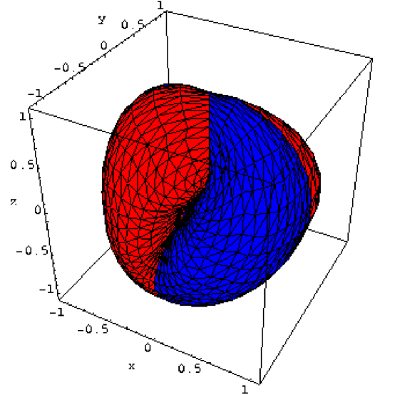
Figure 2: The cross-cap surface

Acknowledgement. I wish to thank Deepak Tolani for very helpful comments, in particular on the use of Bernstein polynomials.

References

• [1] Manfredo P. do Carmo. Differential Geometry of Curves and Surfaces. Prentice Hall, 1976.
• [2] Gerald Farin. NURB Curves and Surfaces, from Projective Geometry to practical use. AK Peters, first edition, 1995.
• [3] Gerald Farin. Curves and Surfaces for CAGD. Academic Press, fourth edition, 1998.
• [4] Jean H. Gallier. Curves and Surfaces In Geometric Modeling: Theory And Algorithms. Morgan Kaufmann, first edition, 1999.
• [5] Ronald Goldman and P.J. Barry. Wonderful triangle: a simple, unified, algorithmic approach to change of basis procedures in computer aided geometric design. In T. Lyche and L.L Schumaker, editors, Mathematical Methods in CAGD II, pages 297–320. Academic Press, 1992.
• [6] D. Hilbert and S. Cohn-Vossen. Geometry and the Imagination. Chelsea Publishing Co., 1952.
• [7] J. Hoschek and D. Lasser. Computer Aided Geometric Design. AK Peters, first edition, 1993.
• [8] S.K. Lodha and Ronald Goldman. Change of basis algorithms for surfaces in CAGD. Computer Aided Geometric Design, 12:801–824, 1995.
• [9] Les Piegl and Wayne Tiller. The NURBS Book. Monograph in Visual Communications. Springer Verlag, first edition, 1995.
• [10] Lyle Ramshaw. Blossoming: A connect-the-dots approach to splines. Technical report, Digital SRC, Palo Alto, CA 94301, 1987. Report No. 19.