Restricted Strip Covering and the Sensor Cover Problem

Abstract

Suppose we are given a set of objects that cover a region and a duration associated with each object. Viewing the objects as jobs, can we schedule their beginning times to maximize the length of time that the original region remains covered? We call this problem the Sensor Cover Problem. It arises in the context of covering a region with sensors. For example, suppose you wish to monitor activity along a fence (interval) by sensors placed at various fixed locations. Each sensor has a range (also an interval) and limited battery life. The problem is then to schedule when to turn on the sensors so that the fence is fully monitored for as long as possible.

This one dimensional problem involves intervals on the real line. Associating a duration to each yields a set of rectangles in space and time, each specified by a pair of fixed horizontal endpoints and a height. The objective is to assign a bottom position to each rectangle (by moving them up or down) so as to maximize the height at which the spanning interval is fully covered. We call this one dimensional problem Restricted Strip Covering. If we replace the covering constraint by a packing constraint (rectangles may not overlap, and the goal is to minimize the highest point covered), then the problem is identical to Dynamic Storage Allocation, a well-studied scheduling problem, which is in turn a restricted case of the well known problem Strip Packing.

We present a collection of algorithms for Restricted Strip Covering. We show that the problem is NP-hard and present an $O(\log\log n)$-approximation algorithm. We also present better approximation or exact algorithms for some special cases. For the general Sensor Cover Problem, we distinguish between cases in which elements have uniform or variable durations. The results depend on the structure of the region to be covered: We give a polynomial-time, exact algorithm for the uniform-duration case of Restricted Strip Covering but prove that the uniform-duration case for higher-dimensional regions is NP-hard. Finally, we consider regions that are arbitrary sets, and we present an $O(\log n)$-approximation algorithm for the most general case.

1 Introduction

Sensors are small, low-cost devices that can be placed in a region to monitor local conditions. Distributed sensor networks have become increasingly more popular as advances in MEMS and fabrication allow for such systems that can perform sensing and communication. How sensors communicate is a well-studied problem. Our main interest is: Once a sensor network has been established, how can we maximize the lifetime of the network? It is clear that the limited battery capacities of sensors is a key constraint in maximizing the lifetime of a network. Additionally, research shows that partitioning the sensors into covers and iterating through them in a round-robin fashion increases the lifetime of the network [1, 3, 8, 9].

Definitions. Let ${\cal S}=\{s_{1},\dots,s_{n}\}$ be a set of sensors. Each sensor $s$ can be viewed as a point in some space with an associated region $R(s)$ of coverage. For every point $x\in R(s)$, $s$ is said to be live at $x$. Let $U$ be the region to be covered by the sensors. $U$ is covered by a collection ${{\cal R}}\subseteq{\cal S}$ of sensors if $U\subseteq\bigcup_{s\in{{\cal R}}}R(s)$. We often refer to ${{\cal R}}$ as a feasible cover. Every sensor $s\in{\cal S}$ can be active for a finite duration $d(s)$. Let $d_{\min}=\min_{s\in{\cal S}}d(s)$, and $d_{\max}=\max_{s\in{\cal S}}d(s)$.

Problem (Sensor Cover).

Compute a schedule $S$ of maximum duration $T$, in which each sensor $s\in{\cal S}$ is assigned a start time $t(s)\geq 0$, such that any $x\in U$ is covered by some active sensor at all times $0\leq t<T$. That is, for all $x\in U$ and $0\leq t<T$, there is some $s\in{\cal S}$ with $x\in R(s)$ and $t(s)\leq t<t(s)+d(s)$.

A sensor is redundant in a schedule $S$ if it can be removed without decreasing the duration of $S$. A schedule with no redundant sensors is a minimal schedule. By removing the redundant sensors, any optimal schedule can be converted to a minimal schedule of the same total duration. Therefore it suffices to consider only minimal schedules, which may not utilize all sensors. As a convention, we set $t(s)=\infty$ if $s$ is unused.

Prior work on the Sensor Cover problem has focused solely on the case where the regions $R(s)$ are arbitrary subsets of $U$ and the durations are all identical. This assumption yields a packing constraint, and the problem reduces to partitioning the set of sensors into a maximum number of valid covers. This problem is known as Set Cover Packing and is $\ln n$-hard to approximate, with a matching upper bound [5].

In practice though, these assumptions appear overly constraining. Sensors will have arbitrary durations and typically define geometric regions of coverage: intervals, rectangles, disks, etc. In this paper, we will consider these classes of problems. In the Restricted Strip Cover problem, all the $R(s)$’s are intervals in one dimension. In this case the problem is equivalent to sliding axis-parallel rectangles vertically to cover a rectangular region of maximum height. Thus, Restricted Strip Cover resembles the Dynamic Storage Allocation (DSA) problem [6], albeit in a dual-like fashion. In the Cube Cover problem, the $R(s)$’s are axis-parallel rectangles, and the problem is akin to sliding cubes vertically in the $z$-dimension. We also consider Sensor Cover, when the $R(s)$’s are arbitrary subsets of a finite set $U$ of size $|U|=O(n)$, with varying durations (in contrast to Set Cover Packing).

In general, a schedule may activate and deactivate a sensor more than once. We call this a preemptive schedule. A non-preemptive schedule is a schedule in which each sensor is activated at most once. In this paper we only consider the non-preemptive problem. We have some preliminary results for the preemptive case, but more research is needed to gain a better understanding of the differences.

Our results. We show that most variants of Sensor Cover are NP-hard, and we study approximation algorithms. For any point $x\in U$, let $L(x)=\sum_{s\in{\cal S},s\text{ live at }x}d(s)$ be the load at $x$ . Define the overall load $L=\min_{x}L(x)$. We write $L_{X}$ (rsp., $L_{X}(x)$) for the load of any subset $X$ of sensors (rsp., at $x$). Letting OPT denote the duration of an optimal schedule, a trivial upper bound is $\text{\it OPT}\leq L$. All our approximation ratios are with respect to $L$. That $\text{\it OPT}\leq L$ allows the assumption that $d_{\max}\leq L$, because durations exceeding $L$ contribute to neither load nor OPT.

Table 1 summarizes our results. The most interesting case is the Restricted Strip Cover problem, for which we give an $O(\log\log n)$-approximation algorithm.

Table 1: Summary of results.

Shape of sensor	Uniform duration	Variable duration
Intervals	exact in P	NP-hard, $O(\log\log n)$-approx.
Rectangles, Disks, …	NP-hard, $O(\ln(n/L))$-approx.	NP-hard, $O(\log n)$-approx.
Arbitrary sets	$\log n$-hard to approx.,	$\log n$-hard to approx.,
	$O(\log n)$-approx. [5]	$O(\log n)$-approx.

After reviewing some related work, we discuss Restricted Strip Cover in Section 2, Cube Cover in Section 3, and the general Sensor Cover problem in Section 4.

Related Work. Set Cover Packing was studied by Feige et al. [5]. They considered the Domatic Number problem, where the goal is to maximize the number of disjoint dominating sets on the set of vertices of a graph. A dominating set in a graph $G=(V,E)$ is a set $V^{\prime}\subset V$ of vertices such that every $v\in V$ is either contained in $V^{\prime}$ or has a neighbor in $V^{\prime}$. Feige et al. show for every $\varepsilon>0$, the Domatic Number problem is hard to approximate within a factor of $(1-\varepsilon)\ln|V|$. In the proof of their hardness result, Feige et al. use the Set Cover Packing problem, whose goal is to maximize the number of disjoint set covers, given a set of subsets $S$ of a base set $U$. Note that the Set Cover Packing problem is a combinatorial version of our problem, with each subset being a region, and each (sensor) region having unit duration. Feige et al. also give a randomized $\ln n$-approximation algorithm, which they derandomize. Another key feature of this work is that it showed the first maximization problem proved to be approximable within polylogarithmic factors but no better.

The practical motivations for studying this problem have led to the development of numerous heuristics. Slijepcevic and Potkonjak [9] introduce the Set K-Cover problem, where they are given a set of subsets of a base set and an integer $k$ and ask if it is possible to construct at least $k$ disjoint set covers. They re-prove an NP-hardness result for this problem, probably unaware of the Feige et al. result. They also present a heuristic that selects mutually exclusive sets of nodes, where each set completely covers the desired region.

Perillo and Heinzelman [8] study a variation of this problem, where they want to maximize the lifetime of a multi-mode sensor network. They compute all possible feasible covers and then translate their problem instance into a graph. Each sensor and feasible cover becomes a node. Sensors are connected to a feasible cover if they are contained in that feasible cover. They use linear programming to model additional energy constraints and solve the maximum flow problem on this graph. Although they solve the problem optimally, their solution can be exponential in the problem instance. Dasika et al. [3] also compute all possible feasible covers and develop heuristics for switching between these covers in order to maximize the lifetime of their sensor network.

Abrams et al. [1] study a variation of the problem where they are given a collection of subsets of a base set and a positive integer $k\geq 2$. Their goal is to partition the subsets into $k$ covers, where the area of coverage, defined as the cardinality of a set, is maximized across all $k$ covers. They give three approximation algorithms for this problem: a randomized algorithm, a distributed greedy algorithm, and a centralized greedy algorithm. Their randomized algorithm partitions sensors within $1-\frac{1}{e}$ of the optimal solution. Their distributed greedy algorithm gives a $\frac{1}{2}$-approximation ratio. Their centralized greedy algorithm achieves an approximation factor of $1-\frac{1}{e}$. They also prove a $\frac{15}{16}$-hardness result for their problem.

To our knowledge, the Restricted Strip Cover problem has not previously been considered. Some of the closely related problems are well studied, however. If we replace the covering constraint by a packing constraint (rectangles may not overlap, and the goal is to minimize the height of the highest point covered), then the problem is the same as Dynamic Storage Allocation [6, Problem SR2], for which there is a $(2+\epsilon)$-approximation [2]. If we further allow rectangles to move both vertically and horizontally, then the problem becomes Strip Packing, which has a $(1+\epsilon)$-approximation (up to an additive term) [7].

2 Restricted Strip Cover

Consider an instance ${\cal S}$ of Restricted Strip Cover (RSC). For ease of presentation, we define $R(s)$ as a semi-closed interval $[\ell(s),r(s))$ for each $s\in{\cal S}$. We assume without loss of generality that all interval coordinates are non-negative integers in the range $[0,2n-1]$ and $U=\bigcup_{s\in{\cal S}}R(s)=[0,2n-1)$, because there are at most $2n$ distinct interval endpoints of sensors. It is convenient to view scheduled sensors as semi-closed rectangles in the plane, with their intervals along the $x$-axis and durations along the $y$-axis. Thus a valid schedule $S$ of duration $T$ is one in which any point $(x,y)$ in the sub-plane $U\times[0,T)$ is covered by some sensor $s$; i.e., $\ell(s)\leq x<r(s)$ and $t(s)\leq y<t(s)+d(s)$. The problem is equivalent to sliding axis-parallel rectangles vertically to cover a rectangular region of maximum height. Therefore, in this section we use the terms “sensor” and “rectangle” interchangeably. We say two or more rectangles overlap if they cover some common point. When discussing multiple schedules, we write $t_{S}(s)$ to denote the start time of $s$ in some schedule $S$; otherwise we omit the subscript.

We also assume that all durations are positive integers. We define level $j$ of any schedule to be the horizontal slice of sensors that cover points at $y$-coordinates in $[j-1,j)$. Let $S$ be some schedule of ${\cal S}$. A gap is a point $p$ such that no sensor covers $p$. For any $i\in U$, define $M(S,i)$ to be the greatest $y$-coordinate $j$ such that no gap exists below $j$ at $i$; i.e., $M(S,i)=\max\{j:\forall j^{\prime}<j,\exists s\in S,\ s\text{ covers }(i,j^{\prime})\}$. Then the duration of $S$ is $M(S)=\min_{i}M(S,i)$.

Our main result for RSC is an $O(\log\log n)$-approximation. En-route we obtain better results for some special cases: (i) a simple, exact algorithm if all sensors have the same duration (Section 2.1); (ii) an exact, dynamic programming algorithm, which runs in $\mathop{\operator@font poly}(n)$ time if $L=O(\log n/\log\log n)$ (Section 2.3); and (iii) $1/(1+\epsilon)$-approximations if $L=O(d_{\min}\log n/\log\log n)$ or $L=\Omega(d_{\max}\log n\cdot(1/\epsilon)^{4}\min\{1/\epsilon,\log(d_{\max}/d_{\min})\})$ (Section 2.4).

Our main technique builds on the method outlined by Buchsbaum et al. [2] in their algorithm for Dynamic Storage Allocation. Their approach does not apply directly, because the covering constraint poses different challenges to solving RSC than does the packing constraint to Dynamic Storage Allocation. We will adapt parts of their method to obtain our bounds.

2.1 Uniform-Duration Sensors

If all sensors have the same duration, a simple greedy algorithm gives an exact solution of duration $L$. Define ${\cal S}_{i}=\{s\in{\cal S}:s\text{ is live at }i\}$. Assume by scaling that all sensors have unit duration. We proceed left-to-right, starting at $i=0$ and constructing a schedule $S$ while maintaining the following invariants after scheduling sensors in ${\cal S}_{i}$: (i) no sensors overlap at any $x$-coordinate $\geq i$, and (ii) $M(S,i)=L$.

When $i=0$, select any $L$ sensors that are live at $0$, and schedule them without overlap, establishing the initial invariants. Assuming the invariants are true at $i$, schedule ${\cal S}_{i+1}$ as follows. If there are no gaps at $i+1$, we are done, as the invariants extend to $i+1$. Otherwise, assume there are $k>0$ unit-duration gaps at $i+1$. The invariants imply that at least $k$ sensors in ${\cal S}_{i+1}$ remain unscheduled, which can be used to fill the gaps while preserving the invariants.

2.2 Hardness Results

When sensors have variable durations, the problem becomes NP-hard. To prove this, we exploit an identity to Dynamic Storage Allocation in a special case. An instance of DSA is like one of RSC, except that the instance load is defined as the maximum load at any $x$-coordinate, and the goal is to schedule the sensors (jobs, in Dynamic Storage Allocation parlance) without overlap so as to minimize the makespan. If the load is equal for all $x$-coordinates, then $\text{\it OPT}=L$ for either problem implies a schedule that is a solid rectangle of height $\text{\it OPT}=L$. For RSC, it further implies that the schedule is non-overlapping; for DSA, this implication is redundant.

Stockmeyer proves that determining if there exists a solution to DSA of a given makespan is NP-complete [6, Problem SR2]. His proof reduces an instance of 3-Partition to an instance of DSA with uniform load and, in fact, all durations in $\{1,2\}$, such that $\text{\it OPT}=L$ if and only if there is a solution to the 3-Partition instance. (See Appendix A for details.) Thus he proves that given a DSA instance with uniform load, determining if $\text{\it OPT}=L$ is NP-complete, even if durations are restricted to the set $\{1,2\}$, and by the above identity, the same is true for RSC.

To establish a gap between OPT and $L$, consider the example in Figure 1, in which $L=4$ but $\text{\it OPT}=3$.

Figure 1: (From Buchsbaum et al. [2].) A set of sensors (in the form $(\ell(\cdot),r(\cdot),d(\cdot))$) $A=(0,1,3)$, $B=(0,3,1)$, $C=(1,2,2)$, $D=(1,4,1)$, $E=(2,3,1)$, $F=(2,5,1)$, $G=(3,4,2)$, and $H=(4,5,3)$. The shaded region is a gap. In this example, $L=4$ but $\text{\it OPT}=3$, which can be realized by sliding $G$ down so that $t(G)=1$.

Scaling the durations shows that no approximation algorithm can guarantee a ratio of better than $4/3$ with respect to $L$.

2.3 A Dynamic Programming Solution for Small $L$

We give a dynamic program to answer the question: Is there a schedule $S$ such that $M(S)=T$ for a fixed $T$? In the following, we ignore portions of sensors that extend above level $T$ in any schedule.

Define ${\cal S}_{\leq i}=\bigcup_{0\leq k\leq i}{\cal S}_{k}$. Consider some schedules $S_{i-1}$ of ${\cal S}_{i-1}$ and $S_{i}$ of ${\cal S}_{i}$ such that $M(S_{i-1},i-1)=M(S_{i},i)=T$. We say that $S_{i-1}$ and $S_{i}$ are compatible if (i) for all $s\in S_{i-1}\cap S_{i},\ t_{S_{i-1}}(s)=t_{S_{i}}(s)$; and (ii) for all $j\in[0,T)$, $(i,j)$ is covered by $S_{i-1}$ or $S_{i}$. The first condition stipulates that any sensor in both schedules must have the same start time in each; the second requires a sensor in $S_{i}$ to be scheduled to cover each level at which coverage stops at $i-1$ in $S_{i-1}$. For each $i$, we populate an array $C_{i}$ indexed by possible schedules of ${\cal S}_{i}$. For any $S_{i}$, define $C_{i}[S_{i}]=1$ if there is a schedule $S$ of ${\cal S}_{\leq i}$ that respects $S_{i}$ and has $M(S,x)=T$ for $0\leq x\leq i$; and $C_{i}[S_{i}]=0$ otherwise. Then $C_{i}[S_{i}]=1$ if and only if $M(S_{i},i)=T$ and there exists some schedule $S_{i-1}$ of ${\cal S}_{i-1}$ such that $C_{i-1}[S_{i-1}]=1$ and $S_{i-1}$ is compatible with $S_{i}$. For $i=0$, $C_{0}[S_{0}]=1$ for precisely those schedules $S_{0}$ of ${\cal S}_{0}$ that have $M(S_{0},0)=T$. The dynamic program then populates the arrays $C_{i}$ in increasing order of $i$, by checking all schedules of ${\cal S}_{i}$ for each $i$. Ultimately we check if there is some schedule $S_{2n-1}$ of ${\cal S}_{2n-1}$ such that $C_{2n-1}[S_{2n-1}]=1$.

First Analysis. For a schedule $S_{i}$ of ${\cal S}_{i}$, consider the union of the rectangles of $S_{i}$, and denote by $\partial(S_{i})$ the vertical boundaries of this union. If $S_{i}$ is part of a minimal schedule $S$ of duration $T$, then any rectangle of $S_{i}$ must cover some point on $\partial(S_{i})$ that is covered by no other rectangles in $S_{i}$. Thus $|S_{i}|\leq 2T$, because $\partial(S_{i})$ has total length $2T$.

Now we can analyze the dynamic program, which we restrict to consider only minimal schedules. The number of sensors in any schedule of ${\cal S}_{i}$ is at most $2T$, so there are at most $\binom{n}{2T}T^{2T}$ possible schedules of ${\cal S}_{i}$, as each potential set of $\eta$ sensors can be scheduled in $T^{\eta}$ ways. Each schedule of ${\cal S}_{i}$ must be checked for compatibility against each schedule of ${\cal S}_{i-1}$, and checking compatibility of a pair of schedules takes $O(T)$ time. Hence the time to run the whole dynamic program is $2n\left(\binom{n}{2T}T^{2T}\right)^{2}O(T)=(nT)^{O(T)}=(nL)^{O(L)}$. To determine OPT, we run the dynamic program for each of the $L$ possible values of $T$, which does not affect the overall asymptotics.

Partitioning the Dynamic Program. Now we restrict the $x$-coordinates on which we have to run the dynamic program to those with relatively few live sensors. Let $X=\{i:|{\cal S}_{i}|<5T\}$. We claim that ${\cal S}$ has a schedule of duration $T$ if and only if ${\cal S}$ has a schedule $S$ such that $M(S,i)\geq T$ for any $i\in X$. We prove the “if” part; the “only if” part is clear.

Assume that there is a minimal schedule $S$ of duration $T$ that only covers $X$. We show how to schedule the sensors not used in $S$ to cover all $x$-coordinates. Consider any maximal interval $\bar{X}$ of $x$-coordinates not in $X$. At most $4T$ sensors from $S$ are live at any $i\in\bar{X}$, because any such sensor is also live at either $\min(\bar{X})-1$ or $\max(\bar{X})+1$, and at most $2T$ are live at either one. By construction, there are at least $5T$ sensors live at any $i\in\bar{X}$, so there are at least $5T-4T=T$ sensors live at $i$ that are not used by $S$ and hence are available, which suffice to cover all the levels at $i$. If such a sensor $s$ should also be live at another $i^{\prime}\in\bar{X}$ (or another $i^{\prime}$ in another $\bar{X^{\prime}}$), it reduces by one both the number of potential uncovered levels and the number of available sensors live at $i^{\prime}$, so enough sensors will remain at $i^{\prime}$.

Therefore we need only run the dynamic program on the $x$-coordinates in $X$. This takes only $2n\cdot T^{O(T)}$ time, because there are fewer than $5T$ sensors live at any $i\in X$. Thus we have:

Theorem 2.1.

RSC can be solved exactly in time $2n\cdot L^{O(L)}$.

Corollary 2.2.

RSC can be solved exactly in $\mathop{\operator@font poly}(n)$ time if $L<c\cdot\log n/\log\log n$ for some constant $c$ small enough.

Using a standard trick, a PTAS follows directly by truncating durations appropriately.

Corollary 2.3.

There is a PTAS for RSC if $L<c\cdot d_{\min}\log n/\log\log n$ for some sufficiently small constant $c$.

2.4 Approximation Algorithms via Grouping

In this section, we give approximation algorithms via the grouping technique, which is similar to the boxing technique of Buchsbaum et al. [2]. We know that the load $L$ is a natural upper bound on OPT, and $L=\text{\it OPT}$ when all sensors have the same duration. The basic idea of grouping is to group shorter sensors into longer, virtual sensors until all the sensors have equal duration, at which point the greedy algorithm is invoked. Essentially we must ensure that the load does not decrease too much during the process, which is the central component of our algorithms.

Grouping Sensors. A grouping of a set $Y$ of sensors into a set of groups $G$ is a partition of $Y$ into $|G|$ subsets, each of which is then replaced by a rectangle that can be covered by the sensors in the group. The duration of a group is defined to be the duration of the rectangle that replaces it. That is, these rectangles can be viewed as sensors in a modified instance. Then $L_{G}$ (rsp., $L_{G}(i)$) is defined to be the load of the groups (rsp., at $i$). Note that $L_{G}(i)\leq L_{Y}(i)$, since portions of the sensors in a group that are overlapped or outside the rectangle are not counted in $L_{G}(i)$. In the following, we give procedures to group a set $Y$ of sensors of unit duration into $G$ such that $L_{G}(i)$ is not much smaller than $L_{Y}(i)$ for any $i$. All of the grouping procedures in this section run in polynomial time.

First, we give a grouping of a set of sensors that are all live at a fixed $x$-coordinate.

Lemma 2.4.

Given a set $Y$ of unit-duration sensors, all live at some fixed $x$-coordinate $x_{0}$, an integer group-duration parameter $D$, and a sufficiently small positive $\epsilon$, there is a set $G$ of groups, each of duration $D$, such that for any $i$,

$$L_{G}(i)>L_{Y}(i)/(1+\epsilon)-4D\lceil 1/\epsilon\rceil.$$

Proof.

It is convenient to view a sensor $s$ as a point $(\ell(s),r(s))$ in the plane. Note that all sensors live at $x_{0}$ are inside the rectangle $R_{x_{0}}=\{(x,y):x\leq x_{0}\leq y\}$ (Figures 2(a)–(b)). First we partition the sensors of $Y$ into strips by repeating the following as long as sensors remain.

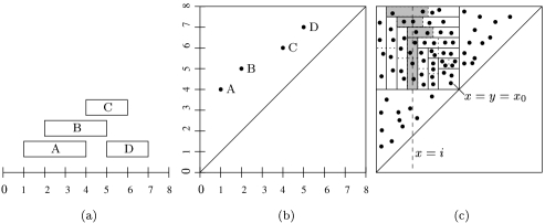
Figure 2: (From Buchsbaum et al. [2].) (a) Four sensors. (b) The sensors of (a) viewed as $(x,y)$ points. (c) Grouping a set of sensors with $D=2$ and $\epsilon=1/2$. The rectangle $R_{i}$ contains the set $Y$ of sensors. The sensors are first partitioned into alternating vertical and horizontal strips of $D\lceil 1/\epsilon\rceil=4$ each. Within each strip, the sensors are grouped (dotted lines) into groups of $D=2$. The groups that intersect the line $x=i$ are shaded.

(1) Create a vertical strip containing the at most $D\lceil 1/\epsilon\rceil$ sensors that remain with the smallest $\ell(\cdot)$ values.

(2) Create a horizontal strip containing the at most $D\lceil 1/\epsilon\rceil$ sensors that remain with the largest $r(\cdot)$ values.

Now for every vertical strip of $Y$, take the sensors in order of decreasing $r(\cdot)$ value in groups of size $D$ (we may discard the last $<D$ sensors in the last strip). Similarly, for every horizontal strip, take the sensors in order of increasing $\ell(\cdot)$ value in groups of size $D$ (we may discard the last $<D$ sensors in the last strip). Replace each group $X$ with a larger rectangle $s_{X}$ with $\ell(s_{X})=\max_{s\in X}\ell(s)$, $r(s_{X})=\min_{s\in X}r(s)$, and $d(s_{X})=\sum_{s\in X}d(s)=D$.

Consider any $i\leq x_{0}$ (the case $i>x_{0}$ is symmetric), and examine Figure 2(c). All sensors live at $i$ are inside the rectangle $R_{i}=\{(x,y):x\leq i\leq y\}$. Assume that the line $x=i$ intersects $k$ horizontal strips; then $R_{i}$ entirely contains at least $k-1$ vertical strips, so $L_{Y}(i)\geq(k-1)D\lceil 1/\epsilon\rceil$. For any group completely inside $R_{i}$, it contributes $D$ to both $L_{Y}(i)$ and $L_{G}(i)$; for any group completely outside $R_{i}$, it does not contribute anything to either $L_{Y}(i)$ or $L_{G}(i)$. So only the groups in the $k$ horizontal strips and the single vertical strip intersected by the line $x=i$ contribute to the difference, that is, $L_{Y}(i)-L_{G}(i)<kD+D\lceil 1/\epsilon\rceil+D$, where the last term accounts for the fewer than $D$ sensors that we did not group in the last strip. Therefore,

$$L_{G}(i)>L_{Y}(i)-(k-1)D-(2+\lceil 1/\epsilon\rceil)D\geq(1-\epsilon)L_{Y}(i)-2D\lceil 1/\epsilon\rceil\geq\frac{1}{1+2\epsilon}L_{Y}(i)-2D\lceil 1/\epsilon\rceil,$$

for any $\epsilon\leq 1/2$. Replacing $\epsilon$ with $\epsilon/2$ gives the desired result. ∎

Next we use Lemma 2.4 to group all sensors of unit duration.

Lemma 2.5.

Given a set $Z$ of unit-duration sensors, an integer group-duration parameter $D$, and a sufficiently small positive $\epsilon$, there is a set $G$ of groups, each of duration $D$, such that at any $x$-coordinate $i$,

$$L_{G}(i)>L_{Z}(i)/(1+\epsilon)-O(\log n\cdot D/\epsilon).$$

Proof.

Build an interval tree ${\cal T}$ on the $x$-projections of the rectangles of $Z$. For each node $v$ of ${\cal T}$, let $Z_{v}$ be the set of sensors associated with $v$. All the sensors of $Z_{v}$ are live at a fixed $x$-coordinate, namely the dividing line at $v$, and thus we can apply Lemma 2.4 to $Z_{v}$ for each $v$.

Consider any $x$-coordinate $i$. For any two different nodes $u,v$ of ${\cal T}$ at the same level, the sensors in $Z_{u}$ and the sensors in $Z_{v}$ do not overlap. Thus the sensors live at $i$ are distributed to at most $O(\log n)$ nodes in ${\cal T}$, because the interval tree has height $O(\log n)$. By Lemma 2.4, we have $L_{G}(i)>\sum_{v\in{\cal T}}(L_{Z_{v}}(i)/(1+\epsilon)-4D\lceil 1/\epsilon\rceil)=L_{Z}(i)/(1+\epsilon)-O(\log n\cdot D/\epsilon)$. ∎

Remark. The $O(\log n)$ factor in the error term of Lemma 2.5 cannot be removed. Consider grouping the example in Figure 3 with $D=2$. First, at least half of sensor A has to be wasted, because it is either grouped with some sensor in the left half or some sensor in the right half. Assume it is grouped with some sensor in the left half. Then by a similar argument, sensor B is cut in half, and one of the halves has to be wasted. Ultimately, we can find an $x$-coordinate $i$ without a single group covering it; i.e., $L_{G}(i)=0$, but $L_{Z}(i)=\Omega(\log n)$.

Figure 3: A bad example

The Algorithm. Let $\epsilon$ be a sufficiently small error parameter, and let $D=d_{\max}\lceil 1/\epsilon\rceil$.

  (1) Truncate each sensor of duration $d$ to $\lceil(1+\epsilon)^{k}\rceil$, where $(1+\epsilon)^{k}\leq d<(1+\epsilon)^{k+1}$ for some integer $k$. Let $X$ be the set of truncated sensors.

  (2) For each $d=\lceil(1+\epsilon)^{k}\rceil,k=\lfloor\log_{1+\epsilon}d_{\min}\rfloor,\dots,\lceil\log_{1+\epsilon}d_{\max}-1\rceil$, do the following. Let $X_{d}$ denote the set of truncated sensors of duration $d$. Scale each sensor in $X_{d}$ down by a factor of $d$, apply Lemma 2.5 with group-duration parameter $\lceil D/d\rceil$ and the given $\epsilon$, and then scale the obtained groups back up by $d$.

  (3) Let $G$ be the set of rectangles obtained from Step (2). Truncate them so that they all have duration exactly $D$. Call the resulting set of rectangles $G^{\prime}$.

  (4) Apply the greedy algorithm to $G^{\prime}$.

Algorithm 1 Approximation algorithm via grouping

Theorem 2.6.

For any sufficiently small positive $\epsilon$, Algorithm 1 runs in $\mathop{\operator@font poly}(n,1/\epsilon)$ time and gives a schedule of the RSC problem with duration at least $L/(1+\epsilon)-O\left(d_{\max}\log n\cdot 1/\epsilon^{3}\log(d_{\max}/d_{\min})\right)$.

Proof.

We will show that the truncating and grouping do not decrease the load at any $i$ excessively.

By Lemma 2.5, Step 2 produces a grouping $G_{d}$ of $X_{d}$ of duration $\lceil D/d\rceil d$ such that at any $i$, $L_{G_{d}}(i)>L_{X_{d}}(i)/(1+\epsilon)-O(\log n\cdot D/\epsilon)$. Summing over all $d$, we have

$$L_{G}(i)>\frac{1}{1+\epsilon}L_{X}(i)-O\left(\frac{D\log n\log(d_{\max}/d_{\min})}{\epsilon\log(1+\epsilon)}\right)=\frac{1}{1+\epsilon}L_{X}(i)-O\left(\frac{d_{\max}\log(d_{\max}/d_{\min})\log n}{\epsilon^{3}}\right).$$

Truncating the sensors in Step (1) decreases their durations by at most $1+\epsilon$, so $L_{X}(i)\geq\frac{1}{1+\epsilon}L(i)$. Truncating the groups in Step (3) decreases their durations by a factor of at most $\frac{\lceil D/d\rceil d}{D}\leq\frac{D+d}{D}\leq 1+\epsilon$, too. Since $\frac{1}{(1+\epsilon)^{3}}\geq\frac{1}{1+7\epsilon}$, we have $L_{G^{\prime}}(i)>L(i)/(1+7\epsilon)-O\left(d_{\max}\log n\cdot 1/\epsilon^{3}\log(d_{\max}/d_{\min})\right)$. Finally, applying the greedy algorithm in Step (4) yields a schedule of duration $\min_{i}L_{G^{\prime}}(i)>L/(1+7\epsilon)-O(d_{\max}\log n\cdot 1/\epsilon^{3}\log(d_{\max}/d_{\min}))$. Replacing $\epsilon$ with $\epsilon/7$ gives the desired result. ∎

Corollary 2.7.

There is a constant $c$ such that for any small enough positive $\epsilon$, the algorithm gives a schedule of duration at least $L/(1+\epsilon)$ for any $L\geq c\cdot d_{\max}\log n\cdot 1/\epsilon^{4}\log(d_{\max}/d_{\min})$.

An Alternative Algorithm. By bootstrapping Steps (1)–(3) of Algorithm 1, we can replace the $O(\log(d_{\max}/d_{\min}))$ factor with $O(1/\epsilon)$, leading to the following result.

Theorem 2.8.

For any sufficiently small positive $\epsilon$, there is an algorithm that runs in $\mathop{\operator@font poly}(n,1/\epsilon)$ time and gives a schedule to the RSC problem with duration at least $L/(1+\epsilon)-O\left(d_{\max}\log n\cdot 1/\epsilon^{4}\right)$.

Proof.

We are going to apply Steps (1)–(3) of Algorithm 1 repeatedly, grouping the smaller sensors so as to increase $d_{\min}$ until $\log(d_{\max}/d_{\min})$ becomes small enough that we can apply Theorem 2.6 to the resulted rectangles.

For ease of presentation, we assume that $1/\epsilon$ is an integer. Let $r$ denote the ratio $d_{\max}/d_{\min}$. Assume first that $\log r\geq 1/\epsilon$, and set $\mu=\epsilon/\log r$ and $D=\lceil\mu^{4}d_{\max}\rceil$. Apply Steps (1)–(3) of Algorithm 1 to ${\cal S}_{s}$, the set of sensors of duration at most $d^{\prime}_{\max}=\lceil\mu D\rceil$, with group duration $D$ and error parameter $\mu$. This yields a set of rectangles $G_{s}$ of duration $D$ such that for any $i$,

$$L_{G_{s}}(i) > \frac{1}{1+\mu}L_{{\cal S}_{s}}(i)-O\left(\frac{d^{\prime}_{\max}\log n\log(d^{\prime}_{\max}/d_{\min})}{\mu^{3}}\right)$$

$$> \frac{1}{1+\mu}L_{{\cal S}_{s}}(i)-O(\mu^{2}d_{\max}\log n\log(\mu^{5}r))>\frac{1}{1+\mu}L_{{\cal S}_{s}}(i)-\frac{c_{1}\epsilon^{2}d_{\max}\log n}{\log r}.~{}~{}~{}\text{($c_{1}$ is some constant.)}$$

Now consider $G_{s}$ as a set of sensors and the new problem instance ${\cal S}^{\prime}=G_{s}\cup({\cal S}\setminus{\cal S}_{s})$. Its load at $i$ is

$$L_{{\cal S}^{\prime}}(i)>\frac{L(i)}{1+\mu}-\frac{c_{1}\epsilon^{2}d_{\max}\log n}{\log r}.$$

Moreover, the new minimum duration of this problem instance is at least $d_{\max}^{\prime}$, and the maximum duration remains $d_{\max}$, so the new ratio is $r^{\prime}\leq\frac{d_{\max}}{d^{\prime}_{\max}}\leq\frac{1}{\mu^{5}}=\frac{\log^{5}r}{\epsilon^{5}}\leq\log^{10}r$, since $\log r\geq 1/\epsilon$. For $\epsilon$ sufficiently small, we have $r^{\prime}\leq\sqrt{r}$; hence $\log r^{\prime}\leq\frac{1}{2}\log r$.

Next repeat the procedure above, each time using new error parameter $\mu^{\prime}=\epsilon/\log r^{\prime}$, until it yields a problem instance ${\cal S}^{*}$ with minimum duration $d^{*}_{\min}$ for which $r^{*}=d_{\max}/d_{\min}^{*}$ is such that $\log r^{*}<1/\epsilon$. Let $r_{0},\dots,r_{k}=r^{*}$ be the sequence of ratios and $L_{0}(i)=L(i),L_{1}(i),\dots,L_{k}(i)=L^{*}(i)$ be the sequence of loads. We have

$$L^{*}(i) > \frac{1}{1+\epsilon/\log r_{k-1}}L_{k-1}(i)-\frac{c_{1}\epsilon^{2}d_{\max}\log n}{\log r_{k-1}}$$

$$> \frac{1}{1+\epsilon/\log r_{k-1}}\left(\frac{1}{1+\epsilon/\log r_{k-2}}L_{k-2}(i)-\frac{c_{1}\epsilon^{2}d_{\max}\log n}{\log r_{k-2}}\right)-\frac{c_{1}\epsilon^{2}d_{\max}\log n}{\log r_{k-1}}$$

$$\cdots$$

$$> \left(\prod_{i=0}^{k-1}\left(1+\frac{\epsilon}{\log r_{i}}\right)\right)^{-1}L(i)-\sum_{i=0}^{k-1}\left(\frac{1}{\log r_{i}}\right)c_{1}\epsilon^{2}d_{\max}\log n$$

$$\geq \frac{1}{1+c_{2}\epsilon/\log r^{*}}L(i)-\frac{2}{\log r^{*}}c_{1}\epsilon^{2}d_{\max}\log n\qquad\text{($c_{2}$ is some constant.)}$$

$$> L(i)/(1+2c_{2}\epsilon^{2})-4c_{1}\epsilon^{3}d_{\max}\log n.$$

Let $L^{*}=\min_{p}L_{{\cal S}^{*}}(i)$. Finally, apply Theorem 2.6 to ${\cal S}^{*}$, which yields a schedule of duration at least

$$\frac{1}{1+\epsilon}L^{*}-O\left(\frac{d_{\max}\log r^{*}\log n}{\epsilon^{3}}\right)\geq\frac{1}{1+c_{4}\epsilon}L-O\left(\frac{d_{\max}\log n}{\epsilon^{4}}\right),$$

for some constant $c_{4}$. Replacing $\epsilon$ with $\epsilon/c_{4}$ gives the desired result. ∎

Corollary 2.9.

There is a constant $c$, such that for any small enough positive real $\epsilon$, the algorithm gives a schedule of duration at least $L/(1+\epsilon)$ for any $L\geq c\cdot d_{\max}\log n\cdot 1/\epsilon^{5}$.

2.5 An $O(\log\log n)$-Approximation for Arbitrary $L$

Theorem 2.8 yields a good approximation only when $d_{\max}$ is small. To extend this, we separate tall rectangles from the short ones and handle the former individually. Henceforth, we will analyze the approximation ratio asymptotically, and we assume that all durations are powers of 2, which at worst halves the duration of the schedule.

Let $d_{\max}=2^{\rho}$, and $\ell=\lceil 2\log\log n\rceil$. We partition ${\cal S}$ into $\ell+1$ subsets ${\cal R}_{0},\dots,{\cal R}_{\ell}$. The first subset ${\cal R}_{0}$ consists of all sensors of duration at most $2^{\rho-\ell}$; then for each $\rho-\ell+1\leq k\leq\rho$, we put all sensors of duration $2^{k}$ into one subset. We call ${\cal R}_{0}$ the small subset and the rest large subsets. For any $x$-coordinate $i$, we compute $L_{{\cal S}_{i}\cap{\cal R}_{k}}(i)$, the load of ${\cal S}_{i}\cap{\cal R}_{k}$ at $i$, for $k=0,\dots,\ell$. Let $m(i)=\mathop{\operator@font argmax}_{k}L_{{\cal S}_{i}\cap{\cal R}_{k}}(i)$; i.e., the sensors in ${\cal S}_{i}\cap{\cal R}_{k}$ have maximum load when $k=m(i)$. Break ties arbitrarily. It is easy to see that the load of ${\cal S}_{i}\cap R_{m(i)}$ is at least $L/(\ell+1)$.

Next, for each $k$, we use ${\cal R}_{k}$ to cover all the $x$-coordinates $i$ where $m(i)=k$, for a duration of $\Omega(L/\log\log n)$. For a large subset ${\cal R}_{k},k\geq 1$, because all its sensors have the same duration, we can use the greedy algorithm to find a schedule of duration at least $L/(\ell+1)=\Omega(L/\log\log n)$. For the small subset ${\cal R}_{0}$, we use Theorem 2.8 with $\epsilon=1$. Since the sensors in ${\cal R}_{0}$ have maximum duration $2^{\rho-\ell}<L/2^{\ell}$, Theorem 2.8 yields a schedule of duration at least

$$\frac{L}{2(\ell+1)}-O\left(\frac{L}{2^{\ell}}\log n\right)\geq\Omega\left(\frac{L}{\log\log n}\right)-O\left(\frac{L}{\log^{2}n}\log n\right)=\Omega\left(\frac{L}{\log\log n}\right).$$

Theorem 2.10.

There exists a polynomial-time $O(\log\log n)$-approximation algorithm for the RSC problem.

3 Cube Cover

3.1 Hardness Results

When the $R(\cdot)$’s are axis-aligned rectangles and $U$ is a two-dimensional region, the problem is NP-hard even when the sensors have uniform duration, in contrast to the uniform-duration case for Restricted Strip Cover. We use a reduction from an instance of NAE-3SAT with $n$ variables and $m$ clauses to an instance of Cube Cover.

An instance $I$ of NAE-3SAT is a set $U=\{u_{1},u_{2},...,u_{n}\}$ of variables and a collection $C=\{C_{1},C_{2},...,C_{m}\}$ of clauses over $U$, such that each clause $C_{i}\in C$ has $|C_{i}|=3$. The problem is to determine if there a truth assignment for $U$ such that each clause in $C$ has at least one true literal and at least one false literal [6]. A key property of NAE-3SAT is that if $X$ is a satisfying assignment for an instance $I$ of NAE-3SAT, $\bar{X}$ is also a satisfying assignment of $I$.

Given $I$, we construct an associated graph $G(I)$, with vertices for each variable and each clause. We draw and edge between a clause vertex and a variable vertex if the variable appears in the clause. The graph is drawn on a planar grid within a bounding box $U$. From $G(I)$, we construct an instance ${\cal S}(I)$ of Cube Cover that has a schedule of duration 2 if and only if $I$ is satisfiable. If $I$ is unsatisfiable, ${\cal S}(I)$ has a schedule of duration 1. We describe the construction in more detail below:

Variables.

Each variable will be represented by a collection of rectangles that cover a square grid. Each rectangle covering the variable gadget has unit duration. The rectangles that cover the variable gadget are shown in Figure 6, arranged in the “true” and “false” encodings. Using a mixture of the rectangles in the “true” and “false” encodings leads to a suboptimal schedule; such a mixture is called an improper cover.

Pipes.

We connect each variable to each clause that contains it via pipes. The pipes are drawn using polygonal lines in the plane. A pipe corresponding to a positive (rsp., negative) occurrence of a variable in a clause leaves via the left (rsp., right) side of the variable gadget. All rectangles that cover a pipe have unit duration. A pipe, as it is drawn within the bounding box, is the leftmost image in Figure 6. To the right of the pipe are the two proper configurations for covering the pipe. The first of the configurations shows how the pipe will be covered when the clause to which it connects is satisfied by the variable assignment. We refer to this as an “on” signal. The second configuration shows how the pipe is covered otherwise. We refer to this as an “off” signal. Using a mixture of rectangles in the two configurations (or an improper cover) will lead to a suboptimal schedule. Figure 6 shows how the variables and pipes connect.

Clauses.

A clause is represented by a square grid at the end of a pipe. A clause is covered if a variable contained in it is satisfied. All other parts of the bounding box are covered with two of the same rectangles, each with unit duration so we can guarantee that every point in $U$, not part of the variable, pipe, or clause gadgets, can be covered for a total of 2 time units.

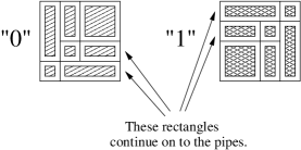
Figure 4: Variables

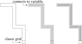
Figure 5: Pipes

Figure 6: Variables and Pipes

In the worst case, each of the variables require a square grid of size $O(m)$, hence the entire grid must contain $O(nm)$ rows and $O(nm)$ columns. Our construction requires $O(n^{2}m^{2})$ unit squares and thus can be performed in polynomial time and space in the size of the input.

Proposition 3.1.

A variable gadget can be covered for two time units using proper covers. If an improper cover is used for $d$ time units, then the gadget can only be covered for $2-d$ time units.

Proof.

Each point in the variable gadget is covered by exactly two rectangles. If proper covers are used, the bounding rectangle can be covered for two units (one for each cover). Note that this is the only way to partition the rectangles into disjoint feasible covers.

Suppose an improper cover is used for $d$ units and the two proper covers are used for $x,y$ time units. Thus the total time for which this rectangle is covered is $x+y+d$. Since at least one rectangle from each proper cover must be in an improper cover, $x+d\leq 1$ and $y+d\leq 1$, and therefore $x+y+d\leq 2-d$. ∎

Proposition 3.2.

The clause square is covered if a variable contained in it is satisfied.

Proof.

If clause $C$ contains variable $u$ and variable $u$ is satisfied in that clause, this means the configuration shown in the middle image of Figure 6 is chosen so the clause grid is covered. ∎

Proposition 3.3.

If $X$ is a satisfying assignment for NAE-3SAT, then $\bar{X}$ is a satisfying assignment as well.

Proof.

If $X$ is a satisfying assignment for NAE-3SAT, then every clause contains at least one variable, $u$, that is true and one variable, $v$, that is false. The complement, $\bar{X}$, makes $u$ false and $v$ true. $\bar{X}$ ensures that every clause contains at least one true variable and one false variable and thus is a satisfying assignment. ∎

Lemma 3.4.

If $I$ is satisfiable, then the instance of Cube Cover has a schedule of duration 2.

Proof.

Let $X$ be a satisfying assignment of $I$. For each variable that is set to 1, choose the “1” orientation for the corresponding variable gadget and the corresponding “on” signal in the pipes connecting this variable to the clauses that contain a positive occurrence of the variable. Choose the “off” signal in pipes connecting this variable to the clauses that contain a negative occurrence of the variable. We repeat this process for variables set to “0”.

Since $X$ is a satisfying assignment, each clause grid will be covered. Moreover, since $\bar{X}$ is also a satisfying assignment, we can repeat this process for another time unit. Note that each pipe is used exactly once to send a “on” signal and once to send a “off” signal, so it can be covered for two time units. Likewise, each variable is used exactly once as “1” and once as “0”, so it can also be covered for two time units. ∎

Lemma 3.5.

If $I$ is unsatisfiable, then the instance of Cube Cover has a schedule of duration at most 1.

Proof.

If all variables are covered using proper covers, we obtain a valid assignment, so some clause rectangle must remain uncovered (since $I$ is unsatisfiable). In order to cover this clause rectangle, we must use an improper cover. Our construction requires that an improper cover creates an overlap either in the variable gadget or the pipes. Since the load at every point in the variable gadget and the pipes is 2 and a rectangle must be used in its entirety or not at all, the maximum schedule has duration 1. ∎

Theorem 3.6.

Cube Cover is NP-hard and does not admit a PTAS, even with uniform duration.

Proof.

NP-hardness follows from Lemma 3.4 and Lemma 3.5.

Assume we have a PTAS ${\cal P}$ for Cube Cover. On input $({\cal S}(I),\epsilon)$, where $\epsilon>0$ and ${\cal S}(I)$ is an instance of Cube Cover induced by the above construction, ${\cal P}$ would output a solution with duration $T$, where $T\geq(1-\epsilon)\cdot OPT$. Setting $\epsilon=0.25$, $T\geq 1.5$ when $OPT=2$, and $0.75\leq T\leq 1$ when $OPT=1$. Thus we can use ${\cal P}$ to distinguish between satisfiable and unsatisfiable instances of NAE-3SAT. ∎

3.2 Rectangles With Unit Duration

We consider approximation algorithms for Cube Cover if all sensors have unit duration. First we prove a technical lemma, which actually holds for arbitrary sets.

Lemma 3.7.

Let $U$ be finite set with $m$ elements. For each $s\in{\cal S}$, $R(s)$ is an arbitrary subset of $U$ with unit duration. There exists some constant $c$ large enough, such that if $L>c\ln m$, then in polynomial time we can find a subset ${\cal R}\subseteq{\cal S}$ and a schedule of ${\cal R}$ with duration at least $L/\ln m$, such that the remaining load $L_{{\cal S}\setminus{\cal R}}\geq L/2$.

Proof.

We take covers from ${\cal S}$ one by one. Let $L_{i}$ be the load of the remaining sensors after the $i^{\text{th}}$ cover has been taken. For the $(i+1)^{\text{th}}$ cover ${\cal X}$, we take each remaining sensor into ${\cal X}$ with probability $p=c\ln m/L_{i}$. Then we check if (1) ${\cal X}$ is a valid cover, and (2) the remaining load $L_{i+1}>L_{i}-\frac{1}{2}\ln m$. For any $x\in U$, the probability that $x$ is not covered is at most $(1-p)^{L_{i}}<m^{-c}$, so (1) occurs with probability at least $1-m^{1-c}$ (probability of union of events). For any $x\in U$, the probability that $L_{i}(x)\leq L_{i}-\frac{1}{2}\ln m$ is at most $m^{-(2c-1)^{2}/8c}$ (Chernoff bound), so (2) occurs with probability at least $1-m^{1-(2c-1)^{2}/8c}$. Thus we can choose $c$ large enough so that both (1) and (2) occur with high probability (e.g., $>1/2$). We repeatedly take ${\cal X}$ until this happens and then proceed to the next cover. We repeat this procedure until $L_{i+1}$ drops below $L/2$, and the lemma follows. ∎

The basic idea of our algorithms is the following. Take a partition of $U$ with a small number of cells, and then crop $R(\cdot)$ so that each sensor fully covers a number of cells but is completely disjoint from the rest. We ensure that the load does not decrease by more than a constant factor and then apply Lemma 3.7.

Theorem 3.8.

If each sensor $s\in{\cal S}$ has unit duration, then there is a polynomial-time $O(\log(n/L))$-approximation algorithm for Cube Cover.

Proof.

We assume $L>c\ln n$ for some large constant $c$; otherwise we just take one cover, and the theorem follows. It is well known that sets of rectangles in the plane admit $(1/r)$-cuttings; there exists a subset ${\cal R}\subset{\cal S}$ of $r\log r$ rectangles such that in the partition ${\cal A}_{{\cal R}}$ determined by the rectangles of ${\cal R}$, each face is intersected by the boundaries of at most $cn/r$ rectangles of ${\cal S}$ [4]. We choose $r=\lceil 2cn/L\rceil$, so $cn/r\leq L/2$.

Let $f$ be a face of ${\cal A}_{{\cal R}}$, and let ${\cal S}_{f}\subseteq{\cal S}$ denote the subset of rectangles that fully contain $f$. Since the load at every point in $f$ is at least $L$ and only $L/2$ rectangles partially cover $f$, we derive $|{\cal S}_{f}|\geq L/2$. Now replace each rectangle $R(s)$ by a cropped region that consists of all faces of ${\cal A}_{{\cal R}}$ that $s$ fully covers. This yields an instance of Sensor Cover, with a universe of size $r^{2}\log^{2}r$ and load $L^{\prime}\geq L/2$. Applying Lemma 3.7 yields the desired result. ∎

An improved bound can be obtained when all the $R(\cdot)$’s have the same size by a more careful cropping scheme.

Theorem 3.9.

If each sensor $s\in{\cal S}$ has unit duration and each $R(s)$ is a unit square, then there is a polynomial-time $O(\log(L_{\max}/L))$-approximation algorithm for Cube Cover, where $L_{\max}=\max_{x}L(x)$. Note that $L_{\max}\leq n$.

Proof.

We assume $L>c\ln L_{\max}$ for some large constant $c$; otherwise we just take one cover, and the theorem follows. We draw a unit-coordinate grid $\Gamma$ inside $U$. There are only $O(n/L)$ cells in $\Gamma$. For a cell $\gamma\in\Gamma$, let ${\cal S}(\gamma)\subseteq{\cal S}$ denote the set of squares of ${\cal S}$ that intersect $\gamma$. Let ${n_{max}}=\max_{\gamma}|{\cal S}(\gamma)|$. Packing arguments imply ${n_{max}}\leq 4L_{\max}$.

Two cells in $\Gamma$ are independent if they are at least two grid cells apart from each other in both dimensions. It is easy to see that we can partition $\Gamma$ into 9 independents sets $\Gamma_{1},\dots,\Gamma_{9}$, where all cells in any one set are mutually independent. In the following, we will show how to make $\Omega(L/\ln({n_{max}}/L))$ covers for $\Gamma_{1}$, such that the remaining load is at least $L/8$. Then we repeat the process for $\Gamma_{2},\dots,\Gamma_{9}$, and ultimately we derive a schedule that covers all cells with duration $\Omega(L/\ln({n_{max}}/L))=\Omega(L/\ln(L_{\max}/L))$.

By the definition of independence, we can isolate the cells in $\Gamma_{1}$ and only need to show that for any $\gamma\in\Gamma_{1}$, we can make $\Omega(L/\ln({n_{max}}/L))$ covers from ${\cal S}(\gamma)$ without decreasing the load of any of its neighboring 8 cells by more than a factor of 8. Since the load of ${\cal S}(\gamma)$ inside $\gamma$ is at least $L$, following the same approach as in the proof of Theorem 3.8, we can build a partition ${\cal A}$ in $\gamma$ and its neighboring cells such that each face of ${\cal A}$ is intersected by the boundaries of at most $L/2$ squares from ${\cal S}(\gamma)$. ${\cal A}$ has size $r^{2}\log^{2}r$, where $r=\lceil 2c{n_{max}}/L\rceil$. We further partition the faces of ${\cal A}$ that are intersected by the boundary of $\gamma$, such that each face of ${\cal A}$ is either inside $\gamma$ or outside. This increases the size of ${\cal A}$ by a factor at most 2. Let ${\cal F}$ be the set of faces of ${\cal A}$ that are fully covered by at least $L/4$ sensors from ${\cal S}(\gamma)$. ${\cal F}$ includes all faces inside $\gamma$ and some faces outside. For any face not in ${\cal F}$, the load of ${\cal S}\setminus{\cal S}(\gamma)$ must be at least $L-L/2-L/4=L/4$, so we can ignore it. Consider the faces in ${\cal F}$. We crop the squares of ${\cal S}(\gamma)$ according to ${\cal F}$ in the same way as in the proof of Theorem 3.8. After cropping, by construction the load at each face of ${\cal F}$ is still at least $L/4$. Then we apply Lemma 3.7 with $U={\cal F}$ and ${\cal S}(\gamma)$, which gives us $\Omega(L/\ln({n_{max}}/L))$ covers while the remaining sensors have load at least $L/8$ for any face of ${\cal A}$. ∎

Remark. These results can be extended to any collection of shapes that admit small cuttings: disks, ellipses, etc.

4 Sensor Cover

Now consider the general Sensor Cover problem, in which each $R(\cdot)$ is an arbitrary subset of a finite set $U$ of size $|U|=O(n)$. We show that a random schedule of the sensors yields an $O(\log n)$-approximation with high probability. This result extends that of Feige et al. [5], which deals with the unit duration case.

Let $T=cL/\ln n$, where $c$ is some constant to be determined later. We show that if we choose the start time of each sensor randomly between 0 and $T$, then we will have a valid schedule with high probability. In order to avoid fringe effects, we must choose positions near 0 or $T$ judiciously. More precisely, for a sensor $s$ of duration $d(s)<T$, we choose its start time $t(s)$ uniformly at random between $-d(s)$ and $T$; if $t(s)<0$, we reset it to 0. If $d(s)\geq T$, we simply set $t(s)=0$. Divide $T$ evenly into $2n$ time intervals $[t_{0}=0,t_{1}],[t_{1},t_{2}],\dots,[t_{2n-1},t_{2n}=T]$, each of length $T/2n$. If $d(s)\geq T/n$, it is easy to see that for any $x\in R(s)$ and in any time interval, $x$ is covered by $s$ with probability at least $(d(s)-T/2n)/(T+d(s))\geq\frac{1}{4}\cdot d(s)/T$.

Consider any $x\in U$, and let $\{s_{1},\dots,s_{k}\}$ be the set of sensors live at $x$ with durations at least $T/n$. We know that $\sum_{i=1}^{k}d(s_{i})\geq L-T/n\cdot n\geq L/2$. In any time interval $[t_{i},t_{i+1}]$, the probability that $x$ is not covered is at most

$$\prod_{i=1}^{k}\left(1-\frac{d(s_{i})}{4T}\right)\leq\prod_{i=1}^{k}\exp\left(-\frac{d(s_{i})}{4T}\right)\leq\exp\left(-\frac{L}{8T}\right)=\exp\left(-\frac{\ln n}{8c}\right)=n^{-\frac{1}{8c}}.$$

There are only $O(n^{2})$ different $(x,[t_{i},t_{i+1}])$ pairs, so the probability that some $x\in U$ is not covered at some time is at most $O(n^{2})\cdot n^{-\frac{1}{8c}}=O\left(n^{2-\frac{1}{8c}}\right)$. Choosing $c<1/16$ yields a high probability of obtaining a valid schedule.

The algorithm can be de-randomized using the method of conditional probability. We omit the details.

It is not hard to see that Set Cover Packing can be reduced to Sensor Cover. Given an optimal schedule produced by an algorithm for Sensor Cover, we can “snap” each starting time $t(s)$ to the integer $\lceil t(s)\rceil$ without introducing any gaps or decreasing the total duration. Hence, the lower bound of Feige et al. [5] applies.

Theorem 4.1.

There exists a polynomial-time $O(\log n)$-approximation algorithm for the Sensor Cover problem. This bound is tight up to constant factors.

5 Conclusions and Open Problems

Many questions remain open. Ideally we would like to prove stronger hardness results or find better approximation algorithms in order to narrow the gap between our lower and upper bounds. In fact, we have not ruled out the possibility of a PTAS for the Restricted Strip Cover problem, although it cannot be in terms of $L$. It would be interesting to see if other techniques for geometric optimization problems could be applied to our problem as well.

We are also interested in understanding preemptive schedules better. For Restricted Strip Cover, a simple algorithm based on maximum flow yields an optimal preemptive schedule in polynomial time. In higher dimensions, however, it is not fully understood in which situations non-preemptive schedules are sub-optimal when compared with the best preemptive schedules. In general, we would like to uncover the relationship between the load of the problem instance, the duration of the optimal preemptive schedule, and the duration of the optimal non-preemptive schedule.

Acknowledgement.

We thank Nikhil Bansal for pointing us to the paper by Kenyon and Remila [7].

Appendix A NP-Completeness of Dynamic Storage Allocation

The following proof was given by Larry Stockmeyer to David Johnson and cited as the “private communication” behind the NP-completeness result in Garey and Johnson [6, Problem SR2]. To our knowledge, this proof has not previously appeared; we include it here essentially verbatim for the more specific results needed in Section 2.2. All credit goes to Larry Stockmeyer. We thank David Johnson for supplying the proof to us.

Dynamic Storage Allocation

Instance: Set $A$ of items to be stored, each $a\in A$ having a size $s(a)$, an arrival time $r(a)$, and a departure time $d(a)$ (with $d(a)>r(a)$), and a positive integer storage size $D$.

Question: Is there an allocation of storage for $A$; i.e., a function $\sigma:A\rightarrow\{1,2,\ldots,D\}$ such that for every $a\in A$ the allocated storage internal $I(a)=[\sigma(a),\sigma(a)+s(a)-1]$ is contained in $[1,D]$ and such that, for all $a,a^{\prime}\in A$ with $a\not=a^{\prime}$, if $I(a)\cap I(a^{\prime})$ is nonempty then $[r(a),d(a))\cap[r(a^{\prime}),d(a^{\prime}))$ is empty?

Theorem: Dynamic Storage Allocation is NP-complete, even when restricted to instances where $s(a)\in\{1,2\}$ for all $a$.

The reduction is from the 3-Partition problem.

3-Partition

Instance: Set $W$ of $3m$ elements, a bound $B$, and a positive integer size $z(w)$ for each $w\in W$, such that $\sum_{w\in W}z(w)=mB$, and $B/4<z(w)<B/2$ for all $w$.

Question: Can $W$ be partitioned into disjoint sets $W_{1},\ldots,W_{m}$ such that, for $1\leq i\leq m$, $\sum_{w\in W}z(w)=B$?

3-Partition is strongly NP-complete [6]; i.e., there is a polynomial $p$ such that it is NP-complete when restricted to instances $I$ where $z(w)\leq p$ (the length of $I$) for all $w$. The condition $B/4<z(w)<B/2$ is not used in the following reduction.

Given an instance of 3-Partition as above, the corresponding instance of Dynamic Storage Allocation has storage size $D=m(B+1)+2$. The instance is described by giving a time-ordered sequence of arrivals and departures of items of various sizes. It is also convenient for the description to allow an item $t$ of size 2 to arrive several times, provided that it first departs before arriving again. Thus, if this item $t$ arrives $k$ times in the entire description, there are really $k$ different items, $t_{i}$ for $1\leq i\leq k$, all of size 2, and no two of them exist at the same time.

In the following, the items $f_{i}$, $g_{i}$, and $h_{i}$ all have size 1. Begin by having $D$ items $f_{1},\ldots,f_{D}$ arrive. Next $f_{1}$ and $f_{2}$ depart, then $t$ arrives and departs, then $g_{1}$ and $g_{2}$ arrive. Now do in sequence for $i=2,3,\ldots,D-1$:

1. items $g_{i}$ and $f_{i+1}$ depart;

2. then item $t$ arrives and departs;

3. then items $h_{i}$ and $g_{i+1}$ arrive.

Finally, $g_{1}$ departs and $h_{1}$ arrives, and then $g_{D}$ departs and $h_{D}$ arrives. At this point, it can be seen that the order of the items in storage must be $h_{1},h_{2},\ldots,h_{D-2},h_{D-1},h_{D}$ or $h_{1},h_{2},\ldots,h_{D-2},h_{D},h_{D-1}$ or the reversal of one of those orderings.

Now $h_{i}$ departs for every $i\leq D-2$ that is not a multiple of $B+1$. At this point, storage consists of $m$ blocks of free space, each block has length $B$, and there are barriers (namely, $h_{B+1}$, $h_{2B+2}$, $\ldots$) between each pair of adjacent blocks.

Consider first the case that sizes of items are not restricted to 1 and 2. For each $w\in W$, an item $q_{w}$ of size $z(w)$ arrives. If the 3-Partition instance has a solution $W_{1},\ldots,W_{m}$, then the items $q_{w}$ with $w\in W_{1}$ can go into the first block of free space, the items $q_{w}$ with $w\in W_{2}$ can go into the second block of free space, and so on for $W_{3},\ldots,W_{m}$.

Conversely, if all the $q_{w}$ fit into the $m$ free blocks of length $B$, then there must be a solution to the 3-Partition instance.

Consider now the case that sizes of items are restricted to 1 and 2. For each $w\in W$, the item $q_{w}$ of size $z(w)$ is replace by $z(w)$ items $q_{w,i}$ for $1\leq i\leq z(w)$, all of size 1. For each $w$, additional arrivals and departures are now added to ensure that the $z(w)$ items $q_{w,i}$ were placed in the same block of free space. The method is similar to the one used above with $f$’s, $g$’s, and $h$’s. First $q_{w,1}$ and $q_{w,2}$ depart, then $t$ arrives and departs, then $q^{\prime}_{w,1}$ and $q^{\prime}_{w,2}$ arrive. The for $i=2,3,\ldots,z(w)-1$: $q^{\prime}_{w,i}$ and $q_{w,i+1}$ depart, then $t$ arrives and departs, then $q^{\prime\prime}_{w,i}$ and $q^{\prime}_{w,i+1}$ arrive. If the $q_{w,i}$ were not placed in the same free block, then at some point the two units of free space formed by the departure of two items must be separated by a barrier, so the item $t$ of size 2 cannot be allocated.

This is a polynomial-time transformation, because the numbers $z(w)$ are bounded above by a polynomial in the length of the 3-Partition instance. Note further that the reduction constructs a Dynamic Storage Allocation instance of uniform load with the ultimate determination being whether $\text{\it OPT}=L$.

References

- [1] Z. Abrams, A. Goel, and S. Plotkin. Set K-cover algorithms for energy efficient monitoring in wireless sensor networks. In Proc. 3rd Int’l. Symp. Information Processing in Sensor Networks (IPSN), pages 424–432, 2004.
- [2] A. L. Buchsbaum, H. Karloff, C. Kenyon, N. Reingold, and M. Thorup. OPT versus LOAD in dynamic storage allocation. SIAM J. Computing, 33(3):632–46, 2004.
- [3] S. Dasika, S. Vrudhula, K. Chopra, and R. Srinivasan. A framework for battery-aware sensor management. In Proc. Design, Automation and Test in Europe Conf. and Expos. (DATE), pages 1–6, 2004.
- [4] M. de Berg and O. Schwarzkopf. Cuttings and applications. Int’l. J. Comp. Geom. & Appl., 5(4):343–355, 1995.
- [5] U. Feige, M. M. Halldórsson, G. Kortsarz, and A. Srinivasan. Approximating the domatic number. SIAM J. Computing, 32(1):172–195, 2002.
- [6] M. R. Garey and D. S. Johnson. Computers and Intractability: A Guide to the Theory of NP-Completeness. W.H. Freeman and Company, 1979.
- [7] C. Kenyon and E. Remila. A near-optimal solution to a two-dimensional cutting stock problem. Math. of Op. Res., 25(4):645–656, 2000.
- [8] M. Perillo and W. Heinzelman. Optimal sensor management under energy and reliability constraints. In Proc. IEEE Wireless Communications and Networking Conf. (WCNC), pages 1621–1626, 2003.
- [9] S. Slijepcevic and M. Potkonjak. Power efficient organization of wireless sensor networks. In Proc. IEEE Int’l. Conf. on Communications (ICC), pages 472–476, June 2001.