Network Inference from Co-Occurrences

Abstract

The discovery of network structures is a fundamental problem in arising in numerous fields of science and technology, communication systems, biology, sociology and neuroscience. Unfortunately, it is often difficult to obtain data that directly reveals network structure, and so one must infer a network from incomplete data. This paper considers inferring network structure from “co-occurrence” data; observations that identify which network components (e.g., switches, routers, genes) carry each transmission but does not indicate the order in which they handle the transmissions. Without order information, there is an exponential number of feasible networks that are compatible with the observed data. Yet, the basic physical principles underlying most networks strongly suggest that all feasible networks are not equally likely. In particular, network elements that co-occur in many observations are probably closely connected. We model the co-occurrence observations as independent realizations of a random walk on the underlying graph, subjected to a random permutation which accounts for the lack of order information. Treating the permutations as missing data, we derive an exact expectation-maximization (EM) algorithm for estimating the random walk parameters. The model and EM algorithm significantly simplify the problem, but the computational complexity of the reconstruction process does grow exponentially in the length of the longest transmission path. For large networks the exact E-step may be computationally intractable, and so we also propose an efficient Monte Carlo EM (MCEM) algorithm, based on importance sampling, and derive conditions which ensure convergence of the algorithm with high probability. Remarkably, the MCEM maintains the desirable properties of the exact EM algorithm and reduces the complexity of each iteration to polynomial-time. Simulations and experiments with Internet measurements demonstrate the promise of this approach.

1 Network Inference and Co-Occurrence Observations

The study of complex networked systems is an emerging field, impacting nearly every area of engineering and science, including the important domains of communication systems, biology, sociology, and cognitive science. The analysis of communication networks enables a better understanding of routing, transmission patterns, and information flow [21, 6]. The analysis of biological networks provides insight into the functional roles played by different genes, proteins, and metabolites in biological systems [13, 19]. The analysis of social networks contributes to a deeper understanding of interactions, dynamics, and the structure of organizations [25, 18]. The analysis of functional connectivity networks in the brain is necessary for the understanding of couplings and interactions between different neuronal colonies [24, 23, 1]. Obtaining or inferring the structure of networks from experimental data precedes any such analysis and is thus a basic and fundamental task, critical to many applications.

Unfortunately, measurements which directly reveal network structure are often beyond experimental capabilities or are excessively expensive. This paper considers inferring network structure from observations that identify which network components (e.g., switches, routers, genes) carry each transmission but does not indicate the order in which they handle the transmissions. Mathematically, the underlying network structure can be represented as a directed graph, and the vertices involved in each transmission form a connected subgraph. The observations only reflect which subset of vertices are involved or “occur” in each transmission; not their inter-connectivity. We refer to such observations as co-occurrences. Co-occurrence observations arise naturally in each of the application areas mentioned above.

Transmissions over telecommunication networks are carried by links and routers/switches which form a path between the source and terminal nodes. In some cases, it is impossible to directly observe the order in which the routers/switches handle each transmission, since sensors are geographically distributed, making precise time-synchronization impractical. The so-called internally-sensed network tomography problem specifically aims at recovering network structure from unordered lists of network elements along transmission paths [21].

Biological signal transduction networks describe fundamental cell functions such as growth, metabolism, differentiation, and apoptosis (disintegration) [19]. Although it is possible to test for individual, localized interactions between genes pairs, such experiments are expensive and time-consuming. High-throughput measurement techniques such as microarrays have successfully been used to identify the components of different signal transduction pathways [28]. However, microarray data only reflects order information at a very coarse, unreliable level. Developing computational techniques for inferring pathway orders is an active research area [16].

Co-occurrence or transactional data also appears in the context of social networks, e.g., by considering which academic papers are co-cited by another paper, which web pages are linked to or from another web page, or which people were diagnosed with a common disease on the same day. Such measurements are readily available, but do not necessarily reflect the temporal or other natural order of occurrence. Researchers in this area have considered the problems of reconstructing networks from co-occurrence data and of using the inferred network to predict potential future co-occurrences [14].

Functional magnetic resonance imaging (fMRI) provides a mechanism for measuring activity in the brain with high spatial resolution. By observing which regions of the brain co-activate while a patient is performing different tasks we can obtain multiple co-occurrence observations. Although fMRI offers high spatial resolution it has limited temporal resolution, making it impractical to obtain complete order information. Magnetoencephalography and electroencephalography measure activity in the brain with higher temporal resolution but only provide coarse spatial resolution, and thus may not allow one to determine precisely which functional regions are active during a given task. Existing techniques for obtaining functional co-activation networks either involve brute-force measurement or use crude correlation methods (see [24] and references therein).

In this article we focus on observations arising from transmissions in a network. Specifically, each co-occurrence observation corresponds to a path through the network. We observe the vertices comprising each path but not the order in which they appear along the path. In certain applications the endpoints (source and destination) of the path may also be observed.

Our goal is to identify which pairs of vertices are directly connected via an edge, thereby learning the structure of the network. A feasible graph is one which agrees with the observations; i.e., a graph which contains a directed path through the vertices in each co-occurrence observation. Given a collection of co-occurrence observations a feasible graph is easily constructed by assigning an order – any order, in fact – to the vertices in each observation, and then inserting directed edges between vertices which are adjacent in the assigned order. In light of the many possible orders for each co-occurrence observation, the number of feasible topologies grows exponentially in the number and size of observations. Without additional assumptions, side information, or prior knowledge, there is no reason to prefer one feasible topology over the others.

Previous work on related problems has involved heuristics using frequencies of co-occurrence either to assign an order to each path [21] or to approximate the probability of transitioning from one vertex to another [14]. These approaches make stringent assumptions and sacrifice flexibility in order to achieve computational tractability and systematically identify a unique solution. The frequency method introduced in [21] is based on a model where paths from a particular source or to a particular destination form a tree. This model coincides with the shortest-path routing policy. When the network provides multiple paths between the same pair of endpoints (e.g., for load-balancing) the algorithm may fail. The cGraph algorithm of Kubica et al. [14] inserts weighted edges between every pair of vertices which co-occur in some observation. This approach produces solutions which are typically much denser than desired. Because both of these methods are based on heuristics, the results they produce are not easily interpreted. Also, these heuristics do not readily lend themselves to incorporating side information. A different approach, introduced by Justice and Hero in [12], involves averaging over an ensemble of feasible topologies sampled uniformly from the feasible set. In general there is an enormous number of feasible topologies (exponential in the problem dimensions) exhibiting a wide variety of characteristics, and it is not clear that an average of feasible topologies will be optimal in any sense. These observations have collectively motivated our development of a more general approach to network reconstruction which we simply term network inference from co-occurrences, or NICO for short.

Our approach is based on a generative model where paths are realizations of a random walk on the underlying graph. A co-occurrence observation is obtained by randomly shuffling each path to account for our lack of observed order information. Based on this model, network inference reduces to estimating the parameters governing the random walk. Then, these parameter estimates determine the most likely order for each co-occurrence.

The following interpretation motivates our shuffled random walk model. Imagine sitting at a particular vertex in the network and observing a series of transmissions pass by. This vertex is only connected to a handful of other vertices in the network, so regardless of its final destination, a transmission arriving at this vertex must pass through one of the neighboring vertices next. Over a period of time, we could record how many arriving transmissions are passed to each neighbor, and then calculate the empirical probabilities of transmissions to each of the neighbors. Obtaining such probabilities at each vertex would provide a tremendous amount of information about the network, but unfortunately co-occurrence observations do not directly reveal them and we therefore face a challenging inverse problem. This paper develops a formal framework for estimating local transition probabilities from a collection of co-occurrence observations, without making any additional assumptions about routing behavior or properties of the underlying network structure. Experimental results on simulated topologies indicate that good performance is obtained for a variety of operating conditions.

It is also worth mentioning that the approach discussed in this paper differs considerably from that of learning the structure of a directed graphical model or Bayesian network, a graph where nodes correspond to random variables and edges indicate conditional independence relationships [9, 8]. A typical aim of graphical modelling is to find a graph corresponding to a factorization of a high-dimensional distribution which predicts the observations well. In turn, these probabilistic models do not directly reflect physical structures, and applying such an approach in the context of this problem would ignore physical constraints inherent to the observations: that co-occurring vertices must lie along a path in the network.

The rest of the paper is organized as follows. In Section 2 we introduce notation and formulate the problem setup. Section 3 reviews the standard approach to estimating the parameters of a random walk when fully observed (ordered) samples are available and presents an EM algorithm for estimating random walk parameters from shuffled observations. A Monte Carlo variant of the EM algorithm is described in Section 4 for situations where long transmission paths make the exact E-step computation prohibitive. Section 5 analyzes convergence of the Monte Carlo EM algorithm. Simulation results are presented in Section 6 and the paper is concluded in Section 7, where ongoing work is also briefly described.

2 Problem Formulation

We model the network as a simple directed graph $G=(S,E)$, where $S=\{1,2,\dots,|S|\}$ is the set of vertices/nodes and $E\subseteq S\times S$ is the set of edges. The number of nodes, $|S|$, is considered known, so network inference amounts to determining the adjacency structure of the graph; that is, identifying whether or not $(i,j)\in E$, for every pair of vertices $(i,j)\in S\times S$.

A co-occurrence observation, ${\bf y}\subset S$, is a subset of vertices in the graph which simultaneously “occur” when a particular stimulus is presented to the network. For example, when a transmission is made over a communication network, a subset of routers and switches carry the transmission from the source to the destination. This activated subset corresponds to a co-occurrence observation, with the stimulus being a transmission between that particular source-destination pair. By repeating this procedure $T$ times with different stimuli we obtain observations, $\mathcal{Y}=\{{\bf y}^{(1)},{\bf y}^{(2)},\dots,{\bf y}^{(T)}\}$, where ${\bf y}^{(m)}=(y_{1}^{(m)},y_{2}^{(m)},\dots,y_{N_{m}}^{(m)})$ is a length-$N_{m}$ co-occurrence, indexed in an arbitrary order.

A directed graph $G=(S,E)$ is said to be feasible with respect to observations $\mathcal{Y}$ if for each co-occurrence ${\bf y}^{(m)}\in\mathcal{Y}$ there exists an ordered path ${\bf z}^{(m)}=(z_{1}^{(m)},z_{2}^{(m)},\dots,z_{N_{m}}^{(m)})$ and a permutation $\mbox{\boldmath$\tau$}^{(m)}=(\tau_{1}^{(m)},\dots,\tau_{N_{m}}^{(m)})$ such that $z_{t}^{(m)}=y_{\tau_{t}^{(m)}}^{(m)}$ for each $t$, and there is an edge from $z_{t-1}$ to $z_{t}$ in the graph for $t=2,\dots,N_{m}$, that is, $(z_{t-1},z_{t})\in E$.

Notice that if we observed ordered paths then network inference would be trivial. We would begin with an empty graph $G_{0}=(S,E)$ with $E=\{\}$. Then, for each ordered observation ${\bf z}^{(m)}$ we would update the set of edges via $E\leftarrow E\cup(z_{t-1}^{(m)},z_{t}^{(m)})$ for $t=2,\dots,N_{m}$. Similarly, if we observed the correct permutation $\mbox{\boldmath$\tau$}^{(m)}$ along with each co-occurrence ${\bf y}^{(m)}$, we could invert the permutation to recover ordered observations and apply the same procedure.

In practice we do not make ordered observations nor do we have access to the correct permutations. However, we can obtain a feasible reconstruction by associating any permutation (of the appropriate length) with each co-occurrence, and then following the procedure described above. There are $N_{m}!$ ways to permute the elements of ${\bf y}^{(m)}$, so there may be as many as $\prod_{m=1}^{T}N_{m}!$ feasible reconstructions. Clearly, for large $N_{m}$ and $T$ this is a huge set to search over. Moreover, without making additional assumptions, or adopting some additional criteria, there is no reason to prefer one feasible reconstruction over another.

Physical principles governing the development of many natural and man-made networks suggest that not all feasible networks are equally plausible. Intuitively, if two or more vertices appear collectively in multiple co-occurrences, we expect that their order is probably the same in the corresponding paths. Likewise, we expect that most vertices will only be directly connected to a small fraction of the other vertices. Based on this intuition we propose the following probabilistic model. First, we model the unobserved, ordered paths, ${\bf z}^{(m)}$, as independent samples of a first-order Markov chain. The Markov chain is parameterized by an initial state distribution $\mbox{\boldmath$\pi$}\in[0,1]^{|S|}$ where $\pi_{i}=P[z_{1}=i]$, and a probability transition matrix, ${\bf A}\in[0,1]^{|S|\times|S|}$, where $A_{i,j}=P[z_{t}=j|z_{t-1}=i]$. Of course, these parameters must satisfy the normalization constraints

$$\sum_{i=1}^{|S|}\pi_{i}=1 \sum_{j=1}^{|S|}A_{i,j}=1,\hskip 14.45377pt\mbox{ for each }i=1,\dots,|S|.$$ and (1)

In addition, we assume that the support of the transition matrix is determined by the adjacency structure of the underlying network; i.e., $A_{i,j}>0$ if and only if $(i,j)\in E$.

A co-occurrence observation, ${\bf y}$, is generated by shuffling the elements of an ordered Markov chain sample, ${\bf z}=(z_{1},\dots,z_{N})$, via a permutation $\tau$ drawn uniformly from $\Psi_{N}$, the collection of all permutations of $N$ elements. Thus, for each $t=1,\dots,N$, $z_{t}=y_{\tau_{t}}$. We assume that $\tau$ is independent of the Markov chain sample, ${\bf z}$. Based on this model, we can write the likelihood of a co-occurrence observation ${\bf y}$ conditioned on the permutation $\tau$ as

$$P[{\bf y}|\mbox{\boldmath$\tau$},{\bf A},\mbox{\boldmath$\pi$}] = \pi_{y_{\tau_{1}}}\prod_{t=2}^{N}A_{y_{\tau_{t-1}},y_{\tau_{t}}}.$$ (2)

Since $P[\mbox{\boldmath$\tau$}]=1/(N!)$, for any $\mbox{\boldmath$\tau$}\in\Psi_{N}$, marginalization over all permutations leads to

$$P[{\bf y}|{\bf A},\mbox{\boldmath$\pi$}]=\frac{1}{N!}\sum_{\mbox{\boldmath$\tau$}\in\Psi_{N}}P[{\bf y}|\mbox{\boldmath$\tau$},{\bf A},\mbox{\boldmath$\pi$}].$$ (3)

Finally, assuming that co-occurrence observations are independent, and taking the logarithm, gives

$$\log P[\mathcal{Y}|{\bf A},\mbox{\boldmath$\pi$}] = \sum_{m=1}^{T}\left[\log\left(\sum_{\mbox{\boldmath$\tau$}\in\Psi_{N_{m}}}P[{\bf y}^{(m)}|\mbox{\boldmath$\tau$}^{(m)},{\bf A},\mbox{\boldmath$\pi$}]\right)-\log(N_{m}!)\right].$$ (4)

Under this model, network inference consists in computing the maximum likelihood (ML) estimates,

$$(\widehat{{\bf A}}_{\mbox{\scriptsize ML}},\widehat{\mbox{\boldmath$\pi$}}_{\mbox{\scriptsize ML}})=\arg\max_{{\bf A},\mbox{\boldmath$\pi$}}\;\log P[\mathcal{Y}|{\bf A},\mbox{\boldmath$\pi$}].$$ (5)

With the ML estimates in hand, we may determine the most likely permutation for each co-occurrence observation according to $({\bf A}_{\mbox{\scriptsize ML}},\mbox{\boldmath$\pi$}_{\mbox{\scriptsize ML}})$, and obtain a feasible reconstruction using our procedure for ordered observations described above.

For non-trivial observations, $\log P[\mathcal{Y}|{\bf A},\mbox{\boldmath$\pi$}]$ is a complicated, non-concave function of $({\bf A},\mbox{\boldmath$\pi$})$, so solving (5) is not a simple task. In the next section, we derive a EM algorithm for solving this optimization problem, by treating the set of permutations, ${\cal T}=\{\mbox{\boldmath$\tau$}^{(1)},...,\mbox{\boldmath$\tau$}^{(T)}\}$, shuffling the paths, as missing data.

3 An EM Algorithm for Estimating Markov Chain Parameters from Shuffled Observations

3.1 Fully Observed Markov Chains: Notation and Estimation

Let $\mathcal{Z}=\{{\bf z}^{(1)},...,{\bf z}^{(T)}\}$ be a set of sample paths, ${\bf z}^{(m)}=(z_{1}^{(m)},...,z_{N_{m}}^{(m)})$, independently generated by a Markov chain with transition matrix ${\bf A}$ and initial state distribution $\pi$ (see (1)). For later use, it is convenient to introduce the equivalent binary representation ${\bf w}^{(m)}=({\bf w}_{1}^{(m)},...,{\bf w}_{N_{m}}^{(m)})$, for each sample ${\bf z}^{(m)}$, defined as follows: ${\bf w}_{t}^{(m)}=(w_{t,1}^{(m)},...,w_{t,|S|}^{(m)})\in\{0,1\}^{|S|}$, with $(w_{t,i}^{(m)}=1)\Leftrightarrow(z_{t}^{(m)}=i)$; of course, one and only one entry of each vector ${\bf w}_{t}^{(m)}$ equals $1$. Finally, let $\mathcal{W}=\{{\bf w}^{(1)},...,{\bf w}^{(T)}\}$, which contains the exact same information as $\mathcal{Z}$. With this notation, we can write

$$\log P[{\cal W}|{\bf A},\mbox{\boldmath$\pi$}] = \sum_{m=1}^{T}\sum_{i=1}^{|S|}w_{1,i}^{(m)}\log\pi_{i}+\sum_{m=1}^{T}\sum_{t=2}^{N_{m}}\sum_{i=1}^{|S|}\sum_{j=1}^{|S|}w_{t-1,i}^{(m)}\,w_{t,j}^{(m)}\log A_{i,j}.$$

$$= \sum_{i=1}^{|S|}\log\pi_{i}\sum_{m=1}^{T}w_{1,i}^{(m)}+\sum_{i=1}^{|S|}\sum_{j=1}^{|S|}\log A_{i,j}\sum_{m=1}^{T}\sum_{t=2}^{N_{m}}\,w_{t-1,i}^{(m)}\;w_{t,j}^{(m)}.$$

Maximum likelihood estimates of $\pi$ and ${\bf A}$ can be obtained from $\mathcal{W}$ my maximizing $\log P[\mathcal{W}|{\bf A},\mbox{\boldmath$\pi$}]$ under the constraints in (1); the solution is well known,

$$\widehat{A}_{i,j}=\frac{\displaystyle\sum_{m=1}^{T}\sum_{t=2}^{N_{m}}\;w_{t-1,i}^{(m)}\;w_{t,j}^{(m)}}{\displaystyle\sum_{j=1}^{|S|}\sum_{m=1}^{T}\sum_{t=2}^{N_{m}}\;w_{t-1,i}^{(m)}\;w_{t,j}^{(m)}},\hskip 28.45274pt\mbox{and}\hskip 28.45274pt\widehat{\pi}_{i}=\frac{1}{T}\sum_{m=1}^{T}w_{1,i}^{(m)}.$$ (6)

3.2 Shufflings, Permutations, and the EM Algorithm

To address the case where we have a set of co-occurrences $\mathcal{Y}=\{{\bf y}^{(1)},\dots,{\bf y}^{(T)}\}$, not ordered samples, we defined the equivalent binary representation $\mathcal{X}=\{{\bf x}^{(1)},\dots,{\bf x}^{(T)}\}$ for $\mathcal{Y}$ in a similar way as above: ${\bf x}^{(m)}=({\bf x}_{1}^{(m)},...,{\bf x}_{N_{m}}^{(m)})$, where ${\bf x}_{t}^{(m)}=(x_{t,1}^{(m)},...,x_{t,|S|}^{(m)})\in\{0,1\}^{|S|}$, with $(x_{t,i}^{(m)}=1)\Leftrightarrow(y_{t}^{(m)}=i)$.

Rather than using $\mbox{\boldmath$\tau$}^{(m)}=(\tau_{1}^{(m)},\dots,\tau_{N}^{(m)})$ to denote the $m$th permutation/shuffling, we introduce a more convenient (binary) representation; each shuffling is represented by a permutation matrix, which we will term shuffling matrix. Let the shuffling matrix for sequence $m$ be denoted as ${\bf r}^{(m)}$ so that $(r_{t,t^{\prime}}^{(m)}=1)\Leftrightarrow(\tau_{t}=t^{\prime})\Leftrightarrow({\bf x}^{(m)}_{t^{\prime}}={\bf w}^{(m)}_{t})\Leftrightarrow(y^{(m)}_{t^{\prime}}=z^{(m)}_{t})$. Given both ${\bf r}^{(m)}$ and ${\bf x}^{(m)}$, we recover the unshuffled sequence ${\bf w}^{(m)}$ by applying (using $0^{0}=1$)

$$w_{t,i}^{(m)}=\prod_{t^{\prime}=1}^{N_{m}}\left(x_{t^{\prime},i}^{(m)}\right)^{r^{(m)}_{t,t^{\prime}}}.$$ (7)

Let ${\cal R}=\{{\bf r}^{(1)},...,{\bf r}^{(T)}\}$ be the collection of shuffling matrices that allow recovering the underlying ordered paths $\mathcal{W}=\{{\bf w}^{(1)},...,{\bf w}^{(T)}\}$ from the corresponding shuffled co-occurrences ${\cal X}=\{{\bf x}^{(1)},...,{\bf x}^{(T)}\}$. We can write the complete log-likelihood $\log P[{\cal X},{\cal R}|{\bf A},{\mbox{\boldmath$\pi$}}]$ as follows:

$$\log P[{\cal X},{\cal R}|{\bf A},{\mbox{\boldmath$\pi$}}] = \log P[{\cal X}|{\cal R},{\bf A},{\mbox{\boldmath$\pi$}}]+\log p[{\cal R}]$$ (9)

$$= \sum_{m=1}^{T}\log P[{\bf x}^{(m)}|{\bf r}^{(m)},{\bf A},{\mbox{\boldmath$\pi$}}]+\log p[{\cal R}]$$

$$= \sum_{m=1}^{T}\;\sum_{t=2}^{N_{m}}\;\sum_{t^{\prime}=1}^{N_{m}}\;\sum_{t^{\prime\prime}=1}^{N_{m}}\;\sum_{i,j=1}^{|S|}\;r^{(m)}_{t,t^{\prime}}\;r^{(m)}_{t-1,t^{\prime\prime}}\;x_{t^{\prime\prime},i}^{(m)}\;x_{t^{\prime},j}^{(m)}\;\log A_{i,j}$$

$$+\sum_{m=1}^{T}\;\sum_{t^{\prime}=1}^{N_{m}}\;\sum_{i=1}^{|S|}\;r^{(m)}_{1,t^{\prime}}\;x_{t^{\prime},i}^{(m)}\;\log\pi_{i}+\log p[{\cal R}],$$

where $p[{\cal R}]$ is the probability of the set of shufflings ${\cal R}$, which we assume constant.

To estimate ${\bf A}$ and $\pi$ from $\mathcal{X}$, we treat $\mathcal{R}$ as missing data, opening the door to the use of the EM algorithm. Notice that if we had the complete data $(\mathcal{X},\mathcal{R})$, we could recover $\mathcal{W}$ via (7) and obtain the closed-form estimates (6). The EM algorithm proceeds by computing the expected value of $\log P[{\cal X},{\cal R}|{\bf A},{\mbox{\boldmath$\pi$}}]$ (w.r.t. $\mathcal{R}$), conditioned on the observations and on the current model estimate $({\bf A}^{k},\mbox{\boldmath$\pi$}^{k})$ (the E-step),

$$Q\left({\bf A},\mbox{\boldmath$\pi$};{\bf A}^{k},\mbox{\boldmath$\pi$}^{k}\right)=E\left[\log P[{\cal X},{\cal R}|{\bf A},{\mbox{\boldmath$\pi$}}]\left|{\cal X},{\bf A}^{k},\mbox{\boldmath$\pi$}^{k}\right.\right].$$ (10)

The model parameter estimates are then updated as follows (the M-step):

$$\left({\bf A}^{k+1},\mbox{\boldmath$\pi$}^{k+1}\right)=\arg\max_{{\bf A},\mbox{\boldmath$\pi$}}\;Q\left({\bf A},\mbox{\boldmath$\pi$};{\bf A}^{k},\mbox{\boldmath$\pi$}^{k}\right).$$ (11)

These two steps are repeated cyclically until a convergence criterion is met.

3.3 The E-step

3.3.1 Sufficient statistics

Rearranging (9), and dropping $\log P[\mathcal{R}]$ (assumed constant), we can write

$$\log P[\mathcal{X},\mathcal{R}|{\bf A},\mbox{\boldmath$\pi$}] \propto \sum_{m=1}^{T}\sum_{i,j=1}^{|S|}\;\;\sum_{t^{\prime},t^{\prime\prime}=1}^{N_{m}}\;\;\sum_{t=2}^{N_{m}}r_{t,t^{\prime}}^{(m)}r_{t-1,t^{\prime\prime}}^{(m)}x_{t^{\prime\prime},i}^{(m)}x_{t^{\prime},j}^{(m)}\log A_{i,j}$$ (12)

$$+\;\sum_{m=1}^{T}\sum_{i=1}^{|S|}\sum_{t^{\prime}=1}^{N_{m}}r_{1,t^{\prime}}^{(m)}x_{t^{\prime},i}^{(m)}\log\pi_{i}.$$

revealing that $\log P[\mathcal{X},\mathcal{R}|{\bf A},\mbox{\boldmath$\pi$}]$ is linear with respect to simple functions of $\mathcal{R}$:

• the first row of each ${\bf r}^{(m)}$: $r^{(m)}_{1,t^{\prime}}$, for $m=1,\dots,T$ and $t^{\prime}=1,\dots,N_{m}$;

• sums of transition indicators: $\alpha^{(m)}_{t^{\prime},t^{\prime\prime}}\equiv\sum_{t=2}^{N_{m}}r^{(m)}_{t,t^{\prime}}\;r^{(m)}_{t-1,t^{\prime\prime}}$, for $m=1,\dots,T$, and $t^{\prime},t^{\prime\prime}=1,\dots,N_{m}$.

Since expectations commute with linear functions, the E-step reduces to computing the conditional expectations of $r^{(m)}_{t,t^{\prime}}$ and $\alpha^{(m)}_{t^{\prime},t^{\prime\prime}}$ (denoted $\bar{r}^{(m)}_{1,t^{\prime}}$ and $\bar{\alpha}^{(m)}_{t^{\prime},t^{\prime\prime}}$, respectively) and plugging them into the complete log-likelihood. Noticing that the $r^{(m)}_{t,t^{\prime}}$ and $\alpha^{(m)}_{t^{\prime},t^{\prime\prime}}$ are binary (in $\{0,\,1\}$), yields

$$\bar{r}^{(m)}_{1,t^{\prime}} = E\left[r^{(m)}_{1,t^{\prime}}\left|{\cal X},{\bf A}^{k},\mbox{\boldmath$\pi$}^{k}\right.\right]\;=\;P\left[r^{(m)}_{1,t^{\prime}}=1\left|{\cal X},{\bf A}^{k},\mbox{\boldmath$\pi$}^{k}\right.\right]$$ (13)

$$\bar{\alpha}^{(m)}_{t^{\prime},t^{\prime\prime}} = E\left[\alpha^{(m)}_{t^{\prime},t^{\prime\prime}}\left|{\cal X},{\bf A}^{k},\mbox{\boldmath$\pi$}^{k}\right.\right]\;=P\left[\alpha^{(m)}_{t^{\prime},t^{\prime\prime}}=1\left|{\cal X},{\bf A}^{k},\mbox{\boldmath$\pi$}^{k}\right.\right].$$ (14)

Finally, $Q\left({\bf A},\mbox{\boldmath$\pi$};{\bf A}^{k},\mbox{\boldmath$\pi$}^{k}\right)$ is obtained simply by plugging $\bar{r}^{(m)}_{1,t^{\prime}}$ and $\bar{\alpha}^{(m)}_{t^{\prime},t^{\prime\prime}}$ in the places of $r^{(m)}_{1,t^{\prime}}$ and $\sum_{t=2}^{N_{m}}r^{(m)}_{t,t^{\prime}}\;r^{(m)}_{t-1,t^{\prime\prime}}$, respectively, in (12).

3.3.2 Computing $\bar{r}^{(m)}_{1,t^{\prime}}$

Since the permutations are (a priori) equiprobable, we have $P[{\bf r}]=1/(N_{m}!)$ (for ${\bf r}\in\Psi_{N_{m}}$), $P\big{[}r_{1,t^{\prime}}^{(m)}=1]=((N_{m}-1)!/N_{m}!)=1/N_{m}$, and $P[{\bf r}|r_{1,t^{\prime}}^{(m)}=1]=1/((N_{m}-1)!)$. Using these facts, together with the mutual independence among the several sequences, and Bayes law, yields

$$\bar{r}^{(m)}_{1,t^{\prime}} = P\left[r^{(m)}_{1,t^{\prime}}=1\left|{\bf x}^{(m)},{\bf A}^{k},\mbox{\boldmath$\pi$}^{k}\right.\right]$$ (15)

$$= \frac{P\big{[}{\bf x}^{(m)}\big{|}r_{1,t^{\prime}}^{(m)}=1,{\bf A}^{k},\mbox{\boldmath$\pi$}^{k}\big{]}\;P\big{[}r_{1,t^{\prime}}^{(m)}=1]}{P[{\bf x}^{(m)}\big{|}{\bf A}^{k},\mbox{\boldmath$\pi$}^{k}\big{]}}$$

$$= \frac{\displaystyle\sum_{{\bf r}\in\Psi_{N_{m}}\!:\;r_{1,t^{\prime}}=1}P\big{[}{\bf x}^{(m)}\big{|}{\bf r},{\bf A}^{k},\mbox{\boldmath$\pi$}^{k}\big{]}}{\displaystyle\sum_{{\bf r}\in\Psi_{N_{m}}}P\big{[}{\bf x}^{(m)}\big{|}{\bf r},{\bf A}^{k},\mbox{\boldmath$\pi$}^{k}\big{]}},$$

where each term $P\big{[}{\bf x}^{(m)}\big{|}{\bf r},{\bf A}^{k},\mbox{\boldmath$\pi$}^{k}\big{]}$ is easily computed after using ${\bf r}$ to unshuffle ${\bf x}^{(m)}$:

$$P\big{[}{\bf x}^{(m)}\big{|}{\bf r},{\bf A}^{k},\mbox{\boldmath$\pi$}^{k}\big{]}=P\big{[}{\bf y}^{(m)}\big{|}\mbox{\boldmath$\tau$},{\bf A}^{k},\mbox{\boldmath$\pi$}^{k}\big{]}=\pi^{k}_{y^{(m)}_{\tau_{1}}}\prod_{t=2}^{N_{m}}A^{k}_{y^{(m)}_{\tau_{t-1}},y^{(m)}_{\tau_{t}}}.$$

Denoting the numerator of (15) as $\gamma_{t^{\prime}}^{(m)}$ we have a more compact expression

$$\bar{r}_{1,t^{\prime}}^{(m)}=\frac{\displaystyle\gamma_{t^{\prime}}^{(m)}}{\displaystyle\sum_{t^{\prime}=1}^{N_{m}}\gamma_{t^{\prime}}^{(m)}}.$$

3.3.3 Computing $\bar{\alpha}_{t^{\prime},t^{\prime\prime}}^{(m)}$

The computation of $\bar{\alpha}_{t^{\prime},t^{\prime\prime}}^{(m)}$ follows a similar path as that of $\bar{r}_{1,t^{\prime}}^{(m)}$; since all permutations are equiprobable, $P[r_{t,t^{\prime}}^{(m)}r_{t-1,t^{\prime\prime}}^{(m)}=1]=(N_{m}-2)!/(N_{m}!)$ and $P[{\bf r}|r_{t,t^{\prime}}^{(m)}r_{t-1,t^{\prime\prime}}^{(m)}=1]=1/((N_{m}-2)!)$, thus

$$\bar{\alpha}_{t^{\prime},t^{\prime\prime}}^{(m)} = \sum_{t=2}^{N_{m}}P\big{[}r_{t,t^{\prime}}^{(m)}r_{t-1,t^{\prime\prime}}^{(m)}=1\big{|}{\bf x}^{(m)},{\bf A}^{k},\mbox{\boldmath$\pi$}^{k}\big{]}$$ (16)

$$= \sum_{t=2}^{N_{m}}\frac{P\big{[}{\bf x}^{(m)}\big{|}r_{t,t^{\prime}}^{(m)}r_{t-1,t^{\prime\prime}}^{(m)}=1,{\bf A}^{k},\mbox{\boldmath$\pi$}^{k}\big{]}\;P\big{[}r_{t,t^{\prime}}^{(m)}r_{t-1,t^{\prime\prime}}^{(m)}=1\big{]}}{P\big{[}{\bf x}^{(m)}\big{|}{\bf A}^{k},\mbox{\boldmath$\pi$}^{k}\big{]}}$$

$$= \sum_{t=2}^{N_{m}}\frac{\displaystyle\left(\frac{1}{(N_{m}-2)!}\sum_{{\bf r}\in\Psi_{N_{m}}:r_{t,t^{\prime}}r_{t-1,t^{\prime\prime}}=1}P\big{[}{\bf x}^{(m)}\big{|}{\bf r},{\bf A}^{k},\mbox{\boldmath$\pi$}^{k}\big{]}\right)\left(\frac{(N_{m}-2)!}{N_{m}!}\right)}{\displaystyle\frac{1}{N_{m}!}\sum_{{\bf r}\in\Psi_{N_{m}}}P\big{[}{\bf x}^{(m)}\big{|}{\bf r},{\bf A}^{k},\mbox{\boldmath$\pi$}^{k}\big{]}}$$

$$= \frac{\displaystyle\sum_{{\bf r}\in\Psi_{N_{m}}}P[{\bf x}^{(m)}|{\bf r},{\bf A}^{k},\mbox{\boldmath$\pi$}^{k}]\sum_{t=2}^{N_{m}}r_{t,t^{\prime}}r_{t-1,t^{\prime\prime}}}{\displaystyle\sum_{{\bf r}\in\Psi_{N_{m}}}P[{\bf x}^{(m)}|{\bf r},{\bf A}^{k},\mbox{\boldmath$\pi$}^{k}]}.$$

Denoting the numerator of (16) as $\gamma_{t^{\prime},t^{\prime\prime}}^{(m)}$, we finally have

$$\bar{\alpha}_{t^{\prime},t^{\prime\prime}}^{(m)}=\frac{\displaystyle\gamma_{t^{\prime},t^{\prime\prime}}^{(m)}}{\displaystyle\sum_{t^{\prime}=1}^{N_{m}}\gamma_{t^{\prime},t^{\prime\prime}}^{(m)}}.$$ (17)

For the $m$th observation, the statistics $\{\bar{r}_{1,t^{\prime}}^{(m)}\}$ and $\{\bar{\alpha}_{t,t^{\prime},t^{\prime\prime}}^{(m)}\}$ have an $O(N_{m}^{2})$ memory cost ($N_{m}^{2}-N_{m}$ transition statistics and $N_{m}$ initial state statistics). These quantities can be computed via the summary statistics $\{\gamma_{t^{\prime}}^{(m)}\}$ and $\{\gamma_{t^{\prime},t^{\prime\prime}}^{(m)}\}$, using the same memory needed to store $\{\bar{r}_{1,t^{\prime}}^{(m)}\}$ and $\{\bar{\alpha}_{t,t^{\prime},t^{\prime\prime}}\}$, in $O\big{(}N_{m}!\big{)}$ operations (the number of all permutations for a length $N_{m}$ observation). For large $N_{m}$, this is a heavy load; Section 4 describes a sampling approach for computing approximations to $\bar{r}_{1,t^{\prime}}$ and $\bar{\alpha}_{t^{\prime},t^{\prime\prime}}$.

3.4 The M-step

Recall that the function $Q\left({\bf A},\mbox{\boldmath$\pi$};{\bf A}^{k},\mbox{\boldmath$\pi$}^{k}\right)$ is obtained by plugging $\bar{r}_{1,t^{\prime}}$ and $\bar{\alpha}_{t^{\prime},t^{\prime\prime}}$ in the places of $r^{(m)}_{1,t^{\prime}}$ and $\sum_{t=2}^{N_{m}}r^{(m)}_{t,t^{\prime}}\;r^{(m)}_{t-1,t^{\prime\prime}}$, respectively, in (12). Maximization w.r.t. ${\bf A}$ and $\pi$, under the constraints in (1), leads to following simple update equations:

$$A^{k+1}_{i,j}=\frac{\displaystyle\sum_{m=1}^{T}\sum_{t^{\prime},t^{\prime\prime}=1}^{N_{m}}\bar{\alpha}_{t^{\prime},t^{\prime\prime}}^{(m)}x_{t^{\prime\prime},i}^{(m)}x_{t^{\prime},j}^{(m)}}{\displaystyle\sum_{j=1}^{|S|}\sum_{m=1}^{T}\sum_{t^{\prime},t^{\prime\prime}=1}^{N_{m}}\bar{\alpha}_{t^{\prime},t^{\prime\prime}}^{(m)}x_{t^{\prime\prime},i}^{(m)}x_{t^{\prime},j}^{(m)}}\;\;\;\mbox{and}\;\;\;\pi_{i}^{k+1}=\frac{\displaystyle\sum_{m=1}^{T}\;\sum_{t^{\prime}=1}^{N_{m}}\;\bar{r}^{(m)}_{1,t^{\prime}}\;x_{t^{\prime},i}^{(m)}}{\displaystyle\sum_{i=1}^{|S|}\sum_{m=1}^{T}\;\sum_{t^{\prime}=1}^{N_{m}}\;\bar{r}^{(m)}_{1,t^{\prime}}\;x_{t^{\prime},i}^{(m)}}.$$ (18)

3.5 Handling Known Endpoints

In some applications, (one or both of) the endpoints of each path are known and only the internal nodes are shuffled. This is the case in communication networks (i.e., internally-sensed network tomography), since the sources and destinations are known, but not the connectivity within the network. In estimation of biological networks (signal transduction pathways), a physical stimulus (e.g., hypotonic shock) causes a sequence of protein interactions, resulting in another observable physical response (e.g., a change in cell wall structure); in this case, the stimulus and response act as fixed endpoints, our goal is to infer the order of the sequence of protein interactions.

Observe that knowledge of the endpoints of each path imposes the constraints

$$r_{1,1}^{(m)}=1\hskip 14.45377pt\mbox{and}\hskip 14.45377ptr_{N_{m},N_{m}}^{(m)}=1.$$

Under the first constraint, estimates of the initial state probabilities are simply given by

$$\widehat{\pi}_{i}=\frac{1}{T}\sum_{m=1}^{T}x_{1,i}^{(m)}.$$

Thus, EM only needs to be used to estimate the transition matrix entries. Let

$$\widetilde{\Psi}_{N}=\{r\in\Psi_{N}\ :\ r_{1,1}=1,\,r_{N,N}=1\},$$

denote the set of permutations of $N$ elements with fixed endpoints. As in the general case, the E-step can be computed using summary statistics (for $t^{\prime},t^{\prime\prime}=1,\dots,N_{m}$)

$$\widetilde{\gamma}^{(m)} = \sum_{r\in\widetilde{\Psi}_{N_{m}}}P[{\bf x}^{(m)}|{\bf r},\widehat{{\bf A}},\widehat{\mbox{\boldmath$\pi$}}]$$

$$\widetilde{\gamma}_{t^{\prime},t^{\prime\prime}}^{(m)} = \sum_{r\in\widetilde{\Psi}_{N_{m}}}\!P[{\bf x}^{(m)}|{\bf r},\widehat{{\bf A}},\widehat{\mbox{\boldmath$\pi$}}]\;\;\sum_{t=2}^{N_{m}}r_{t,t^{\prime}}r_{t-1,t^{\prime\prime}},$$

and setting $\bar{\alpha}_{t^{\prime},t^{\prime\prime}}^{(m)}=\widetilde{\gamma}_{t^{\prime},t^{\prime\prime}}^{(m)}/\widetilde{\gamma}$. The M-step (update for ${\bf A}^{k+1}$) remains unchanged.

3.6 Incorporating Prior Information

The EM algorithm can be easily modified to incorporate conjugate priors; these are Dirichlet priors for $\pi$ and for each row of ${\bf A}$,

$$P[\mbox{\boldmath$\pi$}|{\bf u}]\propto\prod_{i=1}^{|S|}\pi_{i}^{u_{i}-1}\hskip 28.45274pt\mbox{and}\hskip 28.45274ptP[{\bf A}|{\bf v}]\propto\prod_{i=1}^{|S|}\prod_{j=1}^{|S|}A_{i,j}^{v_{i,j}-1},$$ (19)

where the parameters $u_{i}$ and $v_{i,j}$ should be non-negative in order to have proper priors [2]. The larger $u_{i}$ is relative to the other $u_{i^{\prime}}$, $i^{\prime}\neq i$, the greater our prior belief that state $i$ is an initial state rather than the others. Similarly, the larger $v_{i,j}$ relative to other $v_{i,j^{\prime}}$ for $j^{\prime}\neq j$, the more likely we expect, a priori, transitions from state $i$ to state $j$ relative to transitions from $i$ to the other states.

Adding the logarithms of the priors in (19) to the complete log-likelihood (9), we find that incorporating priors into the EM algorithm only results in a change to the M-step. Consider the prior distribution on the initial state distribution; taking $u_{i}=c>1$, for all $i$, has a smoothing effect, encouraging all of the states to have some mass in the initial state distribution. On the other hand, with $0<c<1$ will have a shrinkage effect, encouraging all of the mass to go to one (or a few) of the states. We can push even more aggressively for a sparse solution by choosing negative parameters for the Dirichlet distributions (which will become improper), as done in [7] for Gaussian mixtures. When negative Dirichlet parameters are allowed, the M-step updates become

$$\pi_{i}^{t+1} = \frac{\displaystyle\left(u_{i}+\sum_{m=1}^{T}\sum_{t^{\prime}=1}^{N_{m}}\bar{r}^{(m)}_{1,t^{\prime}}\right)_{+}}{\displaystyle\sum_{i=1}^{|S|}\left(u_{i}+\sum_{m=1}^{T}\sum_{t^{\prime}=1}^{N_{m}}\bar{r}^{(m)}_{1,t^{\prime}}\right)_{+}}$$ (20)

$$A_{i,j}^{k+1} = \frac{\displaystyle\left(v_{i,j}+\sum_{m=1}^{T}\sum_{t^{\prime}=1}^{N_{m}}\sum_{t^{\prime\prime}=1}^{N_{m}}\bar{\alpha}_{t^{\prime},t^{\prime\prime}}^{(m)}x_{t-1,i}^{(m)}x_{t,j}^{(m)}\right)_{+}}{\displaystyle\sum_{j=1}^{|S|}\left(v_{i,j}+\sum_{m=1}^{T}\sum_{t^{\prime}=1}^{N_{m}}\sum_{t^{\prime\prime}=1}^{N_{m}}\bar{\alpha}_{t^{\prime},t^{\prime\prime}}^{(m)}x_{t-1,i}^{(m)}x_{t,j}^{(m)}\right)_{+}}.$$ (21)

where $(a)_{+}=\max\{0,a\}$ is the so-called positive part operator.

4 Monte Carlo E-Step by Importance Sampling

For long sequences, the combinatorial nature of (15) and (16) (involving sums over all permutations of each sequence) may render exact computation impractical. In this section, we consider Monte Carlo approximate versions of the E-step, which avoid the combinatorial nature of its exact version. The Monte Carlo EM (MCEM) algorithm, based on an MC version of the E-step, was originally proposed in [26], and used ever since by many authors (recent work can be found in [11, 3] and references therein).

To lighten the notation in this section, we drop the superscripts from $({\bf A}^{k},\,\mbox{\boldmath$\pi$}^{k})$, using simply $({\bf A},\mbox{\boldmath$\pi$})$ as the current parameter estimates. Moreover, we focus on a particular length-$N$ path ${\bf y}=\{{\bf y}_{1},\dots,{\bf y}_{N}\}\subseteq S^{N}$ and drop the superscript $(m)$; due to the independence of the paths, there’s no loss of generality. Recall that ${\bf y}$ is a (shuffled) path, thus has no repeated elements.

The E-step (see (13) and (14)) consists of computing the conditional expectations $\bar{r}_{1,t^{\prime}}=E\big{[}r_{1,t^{\prime}}\big{|}{\bf x},{\bf A},\mbox{\boldmath$\pi$}\big{]}$ and $\bar{\alpha}_{t^{\prime},t^{\prime\prime}}=E\big{[}\alpha_{t^{\prime},t^{\prime\prime}}\big{|}{\bf x},{\bf A},\mbox{\boldmath$\pi$}\big{]}$. A naïve Monte Carlo approximation would be based on random permutations, sampled from the uniform distribution over $\Psi_{N}$. However, the reason to resort to approximation techniques in the first place is that $\Psi_{N}$ is large, with only a small fraction of these random permutations having non-negligible posterior probability, $P[{\bf r}|{\bf x},{\bf A},\mbox{\boldmath$\pi$}]$; a very large number of uniform samples is thus needed to obtain a good approximation to $\bar{r}_{1,t^{\prime}}$ and $\bar{\alpha}_{t^{\prime},t^{\prime\prime}}$.

Ideally, we would sample permutations directly from the posterior $P[{\bf r}|{\bf x},{\bf A},\mbox{\boldmath$\pi$}]$; however, this would require determining its value for all $N!$ permutations. Instead, we employ importance sampling (IS) (see, e.g., [22, 15], for an introduction to IS): we sample $L$ permutations, ${\bf r}^{1},\dots,{\bf r}^{L}$, from a distribution $R[{\bf r}|{\bf x},{\bf A},\mbox{\boldmath$\pi$}]$, from which it is easier to sample than $P[{\bf r}|{\bf x},{\bf A},\mbox{\boldmath$\pi$}]$, then apply a corrective re-weighting to obtain approximations to $\bar{r}_{1,t^{\prime}}$ and $\bar{\alpha}_{t^{\prime},t^{\prime\prime}}$ (note that we are now using superscripts on ${\bf r}$ to index sample numbers, not to identify paths). The IS estimates are given by

$$\bar{r}_{1,t^{\prime}} \simeq \frac{\displaystyle\sum_{i=1}^{L}z_{i}\;r_{1,t^{\prime}}^{i}}{\displaystyle\sum_{i=1}^{L}z_{i}},$$ (22)

$$\bar{\alpha}_{t,t^{\prime},t^{\prime\prime}} \simeq \frac{\displaystyle\sum_{i=1}^{L}z_{i}\;\sum_{t=2}^{N_{m}}r_{t,t^{\prime}}^{i}\;r_{t-1,t^{\prime\prime}}^{i}}{\displaystyle\sum_{i=1}^{L}z_{i}},$$ (23)

where $z_{i}$, the correction factor (or weight) for sample ${\bf r}^{i}$, is given by

$$z_{i}=\frac{P[{\bf r}^{i}|{\bf x},{\bf A},\mbox{\boldmath$\pi$}]}{R[{\bf r}^{i}|{\bf x},{\bf A},\mbox{\boldmath$\pi$}]},$$ (24)

the ratio between the desired distribution and the sampling distribution employed.

A relevant observation is that the target and sampling distributions only need to be known up to normalizing factors. Given $R^{\prime}[{\bf r}]=Z_{R}\,R[{\bf r}|{\bf x},{\bf A},\mbox{\boldmath$\pi$}]$ and $P^{\prime}[{\bf r}|{\bf x},{\bf A},\mbox{\boldmath$\pi$}]=Z_{P}\,P[{\bf r}|{\bf x},{\bf A},\mbox{\boldmath$\pi$}]$, for constants $Z_{R}$ and $Z_{P}$, we can use

$$z^{\prime}_{i}=\frac{P^{\prime}[{\bf r}^{i}|{\bf x},{\bf A},\mbox{\boldmath$\pi$}]}{R^{\prime}[{\bf r}^{i}|{\bf x},{\bf A},\mbox{\boldmath$\pi$}]}=\frac{Z_{P}}{Z_{R}}\;z_{i},$$ (25)

instead of $z_{i}$ in (22) and (23); these sums will remain unchanged since the factor $Z_{P}/Z_{R}$ will appear both in the numerator and denominator, thus cancelling out.

The remainder of this section contains the description of an IS scheme, including the derivation of closed form expressions for both the sampling distribution, $R$, and the sample weights, $z_{i}$. We conclude the section by mentioning other sampling variants and presenting experimental results.

4.1 Sampling Scheme

Let ${\bf f}=\{f_{1},\dots,f_{|S|}\}\in\{0,1\}^{|S|}$ be a sequence of binary flags. Given some probability distribution $\mathbf{p}=\{p_{1},p_{2},\dots,p_{|S|}\}$ on the set of states, $S$, denote by $\mathbf{p}\cdot{\bf f}$ the restriction of $\mathbf{p}$ to those elements of $S$ that have corresponding flag $f_{i}$ set to 1, that is,

$$(\mathbf{p}\cdot{\bf f})_{i}=\frac{\displaystyle p_{i}\;f_{i}}{\displaystyle\sum_{j=1}^{|S|}p_{j}\;f_{j}},\hskip 14.45377pt\mbox{for}\ i=1,2,\dots,|S|.$$ (26)

The proposed sampling scheme is defined as follows:

Step 1:

Let ${\bf f}=\{f_{1},\dots,f_{|S|}\}$ be initialized according to $f_{i}=\mathbb{I}_{\{i\in{\bf y}\}},$ where $\mathbb{I}_{\{\}}$ denotes the indicator function.

Obtain one sample from $S$ according to the distribution $\mbox{\boldmath$\pi$}\cdot{\bf f}$. Let the obtained sample be denoted $s$; of course, one and only one element of ${\bf y}$ is equal to $s$.

Locate the position $t$ of $s$ in ${\bf y}$; that is, find $t$ such that $y_{t}=s$. Set $\tau_{1}=t$.

Set $f_{s}=0$ (preventing $y_{t}$ from being sampled again). Set $i=2$.

Step 2:

Let $\mathbf{p}=\{A_{s,1},\dots,A_{s,|S|}\}$ be the $s$th row of the transition matrix.

Obtain a sample $s^{\prime}$ from $S$, according to the distribution $\mathbf{p}\cdot{\bf f}$.

Find $t$ such that $y_{t}=s^{\prime}$. Set $\tau_{i}=t$. Set $f_{s^{\prime}}=0$.

Step 3:

If $i<N$, then set $s\leftarrow s^{\prime}$, set $i\leftarrow i+1$, go back to Step 2; otherwise, stop.

4.1.1 Sampling Distribution

Before deriving the form of the distribution $R$, let us begin by writing the target distribution $P[\mbox{\boldmath$\tau$}|{\bf y},{\bf A},\mbox{\boldmath$\pi$}]$ explicitly. Using Bayes law,

$$P[\mbox{\boldmath$\tau$}|{\bf y},{\bf A},\mbox{\boldmath$\pi$}]=\frac{P[{\bf y}|\mbox{\boldmath$\tau$},{\bf A},\mbox{\boldmath$\pi$}]P[\mbox{\boldmath$\tau$}]}{P[{\bf y}|{\bf A},\mbox{\boldmath$\pi$}]},$$ (27)

since $\tau$ does not depend a priori on ${\bf A}$ or $\pi$. Based on our assumption that all permutations are equiprobable we have $P[\mbox{\boldmath$\tau$}]=\mathbb{I}_{\{\mbox{\boldmath$\tau$}\in\Psi_{N}\}}/N!$. Noticing that the denominator in (27) is just a normalizing constant independent of $\tau$, we have

$$P[\mbox{\boldmath$\tau$}|{\bf y},{\bf A},\mbox{\boldmath$\pi$}]\propto\mathbb{I}_{\{\mbox{\boldmath$\tau$}\in\Psi_{N}\}}\ P[{\bf y}|\mbox{\boldmath$\tau$},{\bf A},\mbox{\boldmath$\pi$}]=\mathbb{I}_{\{\mbox{\boldmath$\tau$}\in\Psi_{N}\}}\left(\pi_{y_{\tau_{1}}}\prod_{t=2}^{N}A_{y_{\tau_{t-1}},y_{\tau_{t}}}\right).$$ (28)

For the sake of notational economy, we will write simply $R[\mbox{\boldmath$\tau$}]$ to represent $R[\mbox{\boldmath$\tau$}|{\bf y},{\bf A},\mbox{\boldmath$\pi$}]$. The sequential nature of the sampling scheme suggests a factorization of the form

$$R[\mbox{\boldmath$\tau$}]=R[\tau_{1}]\;R[\tau_{2}|\tau_{1}]\;R[\tau_{3}|\tau_{2},\tau_{1}]\;\cdots\;R[\tau_{N}|\tau_{N-1},\dots,\tau_{1}].$$ (29)

For Step 1 of the sampling scheme, it’s clear that, for $\tau_{1}=1,\dots,N$,

$$R[\tau_{1}]\propto\pi_{y_{\tau_{1}}}.$$ (30)

For the $i$-th iteration, we have,

$$R[\tau_{i}|\tau_{i-1},\dots,\tau_{1}]=A_{y_{\tau_{i-1}},y_{\tau_{i}}}\;\phi_{i}(\tau_{i-1},\dots,\tau_{1})\;\mathbb{I}_{\{\tau_{i}\notin\{\tau_{i-1},\dots,\tau_{1}\}\}},$$ (31)

with

$$\phi_{i}(\tau_{i-1},\dots,\tau_{1})=\left(\sum_{t\notin\{\tau_{i-1},\dots,\tau_{1}\}}A_{y_{\tau_{i-1}},y_{t}}\right)^{-1}.$$

Inserting (30) and (31) into (29), we finally have

$$R[\mbox{\boldmath$\tau$}]\propto\left[\pi_{y_{\tau_{1}}}\prod_{i=2}^{N}A_{y_{\tau_{i-1}},y_{\tau_{i}}}\right]\left[\prod_{i=2}^{N}\phi_{i}(\tau_{i-1},\dots,\tau_{1})\right]\left[\prod_{i=2}^{N}\mathbb{I}_{\{\tau_{i}\notin\{\tau_{i-1},\dots,\tau_{1}\}\}}\right];$$ (32)

observe that the third factor in the r.h.s. of (32) is simply the indicator that $\tau$ is a permutation, i.e., is equal to $\mathbb{I}_{\{\mbox{\boldmath$\tau$}\in\Psi_{N}\}}$, for any $\mbox{\boldmath$\tau$}\in\{1,...,N\}^{N}$.

Dividing (28) by (32) we obtain the correction factor $z$ for a permutation sample $\tau$ generated using this sequential scheme as

$$z=\left(\prod_{i=2}^{N}\phi_{i}(\tau_{i-1},\dots,\tau_{1})\right)^{-1}=\prod_{i=2}^{N}\;\;\sum_{t\notin\{\tau_{i-1},\dots,\tau_{1}\}}A_{y_{\tau_{i-1}},y_{t}}.$$ (33)

With this quantity in hand, we have all the ingredients needed to produce IS estimates of $\bar{r}_{1,t^{\prime}}$ and $\bar{\alpha}_{t,t^{\prime},t^{\prime\prime}}$. Notice that computing the terms $\phi_{i}$, thus computing $z$, is easy since these factors are the normalization terms for the distributions $\mathbf{p}\cdot{\bf f}$, which are already computed while performing each iteration of Step 2. Thus, we just need to store the product of these normalizing constants to finally obtain the weight $z$.

4.1.2 Known Endpoints

In the case where the endpoints are known, we fix $\tau_{1}=1$, $\tau_{N}=N$, and set $f_{1}=0$ and $f_{N}=0$ in Step 1; the remainder of the procedure is unchanged. Based on these constraints, the importance sampling weight takes a slightly different form:

$$z=\pi_{y_{1}}\;A_{y_{\tau_{N-1}},y_{N}}\;\prod_{i=2}^{N-1}\sum_{t\notin\{\tau_{i-1},\dots,\tau_{1}\}}A_{y_{\tau_{i-1}},y_{t}}.$$ (34)

4.2 Hierarchical Sampling Schemes

In addition to the sampling scheme that we have just described, we have also developed other sampling schemes that work in a hierarchical, rather than sequential, fashion. For the sake of space, we refrain from describing these other sampling schemes; detailed descriptions can be found in [20]. In particular, we have developed a two-stage hierarchical scheme and a fully hierarchical scheme. In the two-stage method, the first stage samples from the collection of all possible transitions occurring in a path; then the second stage samples from the distribution on all arrangements of these transitions, to form a permutation. In the fully hierarchical method, the first stage samples a suitable set of transitions, say ${\cal G}_{1}$; then, the following stage samples a suitable collection of pairs of elements of ${\cal G}_{1}$, yielding a collection of quadruples, ${\cal G}_{2}$, and the procedure is repeated until a permutation is obtained.

4.3 Performance Assessment

A standard error metric for comparing two distributions $P$ and $\widehat{P}$ taking values on the finite set $\Psi_{N}$ is the $\ell_{1}$ distance, defined as

$$\|P-\widehat{P}\|_{1}=\sum_{{\bf r}\in\Psi_{N}}\left|P[{\bf r}]-\widehat{P}[{\bf r}]\right|.$$ (35)

Given a set of permutations, $\{{\bf r}^{1},\dots,{\bf r}^{L}\}$, drawn from the sampling distribution $R$ along with the corresponding weights, $z_{1},\dots,z_{L}$, we can compute the empirical distribution $\widehat{P}_{R}$ induced on $\Psi_{N}$ according to

$$\widehat{P}_{R}[{\bf r}]=\left(\sum_{i=1}^{L}z_{i}\right)^{-1}\sum_{i=1}^{L}\;z_{i}\;\mathbb{I}_{\{{\bf r}^{i}={\bf r}\}}.$$ (36)

Notice that the Monte Carlo sufficient statistics $\widehat{\alpha}_{t^{\prime},t^{\prime\prime}}^{(m)}$ and $\widehat{r}_{1,t^{\prime}}^{(m)}$ are just sums of terms $\widehat{P}_{R}[{\bf r}]$, e.g., $\widehat{\alpha}_{t^{\prime},t^{\prime\prime}}=\sum_{{\bf r}\in\Psi_{N}}\widehat{P}_{R}[{\bf r}]\sum_{t=2}^{N_{m}}r_{t-1,t^{\prime\prime}}r_{t,t^{\prime}}$. Thus,

$$\left|\bar{\alpha}_{t^{\prime},t^{\prime\prime}}^{(m)}-\widehat{\alpha}_{t^{\prime},t^{\prime\prime}}^{(m)}\right|\leq\left\|P-\widehat{P}_{R}\right\|_{1}\hskip 28.45274pt\mbox{and}\hskip 28.45274pt\left|\bar{r}_{1,t^{\prime}}^{(m)}-\widehat{r}_{1,t^{\prime}}^{(m)}\right|\leq\left\|P-\widehat{P}_{R}\right\|_{1},$$

showing that if the $\ell_{1}$ error between the true distribution on permutations and the empirical importance sampling distribution is small, then all of the estimated sufficient statistics will be close to the corresponding exact value.

We have evaluated the performance of various sampling schemes via simulation, considering three scenarios concerning the distribution over all permutations: 1) roughly uniform, 2) moderately peaked, and 3) highly concentrated around just a few permutations. The scenario 1) is typical of the first EM iterations; scenario 2) is typical during intermediate EM iterations; the third scenario is typical when EM is near convergence. We consider a length-8 path with known endpoints, thus with $6!=720$ possible orderings. This length is long enough to suggest how each sampling scheme will perform for longer paths, while still allowing enumeration of all orderings.

Figure 1 depicts the $\ell_{1}$ error between the true and IS-based distributions on permutations, as a function of the number of samples. The curve labelled “True Dist” corresponds to sampling from the true distribution, shown as a reference, is only possible when we can enumerate all permutations. The “Causal IS” curve corresponds to the scheme described in Section 4.1. The “Two Stage” and “Hierarchical” curves depict the performance for the hierarchical schemes mentioned in Section 4.2. Finally, “Random” refers to an approach where we sample from a uniform distribution on permutations, shown as a baseline comparison. Each curve was generated by averaging over 50 Monte Carlo simulations. These curves depict performance using up to 500 samples for a path with 720 possible orderings, which is actually quite a generous helping of samples. In experiments with Internet data we have encountered paths of up to length 27, and observed good reconstruction performance using as few as $2000$ samples (notice that $27!\simeq 10^{28}$). Thus, performance for very few samples is of great interest. As expected, all of the sampling schemes give the same performance when distribution is roughly uniform. However, as the distribution becomes more concentrated, there is a clear difference between the various sampling schemes. The uniform sampling scheme naturally performs the worst on more concentrated distributions. Of the schemes that are practical for long paths, these results indicate that the causal sampling scheme performs the best.

In terms of computational complexity, the causal sampler is the simplest and fastest, requiring only $O(N)$ operations per sample ($N$ is the path length). The two-stage sampler requires $O\big{(}(N/2)!\big{)}$ operations per sample, while the fully hierarchical has computational complexity $O(N^{2}\log N)$ operations per sample. The conclusion is that the causal sampling method described above is simple to implement, fast, and it empirically outperforms more computationally complex schemes.

Figure 1: $\ell_{1}$ error as a function of the number of importance samples drawn for various sampling schemes in the following scenarios: (a) a roughly uniform distribution on the permutations, (b) moderately peaked distribution, (c) highly concentrated distribution. The curves in each figure were calculated by averaging over 50 Monte Carlo simulations.

To compare the efficacy of each sampling scheme within the EM algorithm, we generated a random network with 250 nodes and simulated 60 random sample paths through this network, ranging in length from 4 to 10 hops. Then, we estimated a probability transition matrix for the network using the EM algorithm with different IS-based E-steps (with known endpoints for each path). Figure 2 depicts the marginal log-likelihood of the data, computed according to (4) using the probability transition matrices returned by the EM algorithm, for a number of samples-per-path between 20 and 100. The horizontal dashed line at the top marks the marginal log likelihood computed using a transition matrix estimated from correctly ordered paths.

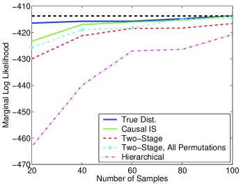
Figure 2: Using various approximate E-steps in the EM algorithm for estimating the Markov transition matrix of a simulated network. The horizontal dashed line at the top of the figure marks the marginal log likelihood of the data using the transition matrix derived using the correctly ordered paths. The curves in this figure correspond to the average over 10 Monte Carlo simulations.

5 Monotonicity and Convergence

Well-known convergence results due to Wu and Boyles [27, 4] guarantee convergence of our EM algorithm when the exact E-step is used. Let $\mbox{\boldmath$\theta$}^{k}=\big{(}{\bf A}^{k},\mbox{\boldmath$\pi$}^{k}\big{)}$ denote parameter estimates calculated at the $k$th EM iteration using the exact EM expressions. By choosing $\mbox{\boldmath$\theta$}^{k+1}=\big{(}{\bf A}^{k+1},\mbox{\boldmath$\pi$}^{k+1}\big{)}$ according to (11) in the M-step, our iterates satisfy the monotonicity property:

$$Q\left(\mbox{\boldmath$\theta$}^{k+1};\mbox{\boldmath$\theta$}^{k}\right) \geq Q\left(\mbox{\boldmath$\theta$}^{k};\mbox{\boldmath$\theta$}^{k}\right).$$ (37)

The marginal log-likelihood (4) is continuous in its parameters ${\bf A}$ and $\pi$ and it is bounded above. In this setting the monotonicity property (37) guarantees that each exact EM update monotonically increases the marginal log-likelihood, so the EM iterates converge to a local maximum.

When Monte Carlo methods are used in the E-step monotonicity is no longer guaranteed since the M-step solves

$$\widehat{}\mbox{\boldmath$\theta$}^{k+1}\equiv\big{(}\widehat{{\bf A}}^{k+1},\widehat{}\mbox{\boldmath$\pi$}^{k+1}\big{)} = \arg\max_{{\bf A},\mbox{\boldmath$\pi$}}\widehat{Q}\big{(}{\bf A},\mbox{\boldmath$\pi$};{\bf A}^{k},\mbox{\boldmath$\pi$}^{k}\big{)},$$

where $\widehat{Q}$ is defined analogously to $Q$ but with terms $\bar{\alpha}_{t^{\prime},t^{\prime\prime}}^{(m)}$ and $\bar{r}_{1,t^{\prime}}^{(m)}$ replaced by $\widehat{\alpha}_{t^{\prime},t^{\prime\prime}}^{(m)}$ and $\widehat{r}_{1,t^{\prime}}^{(m)}$, their corresponding importance sampling approximations. Consequently, care must be taken to ensure that $\widehat{Q}$ approximates $Q$ well enough so that the EM algorithm is not swamped with error from the Monte Carlo estimates.

To illustrate this issue, consider the following synthetic example. We generate 40 co-occurrence observations by taking a random walk on a graph with 140 vertices. Each co-occurrence has between 4 and 8 vertices. Figure 3(a) plots $Q(\mbox{\boldmath$\theta$}^{k};\mbox{\boldmath$\theta$}^{k-1})$ for the exact E-step, along with $\widehat{Q}(\widehat{}\mbox{\boldmath$\theta$}^{k+1};\widehat{}\mbox{\boldmath$\theta$}^{k})$ and $Q(\widehat{}\mbox{\boldmath$\theta$}^{k+1};\widehat{}\mbox{\boldmath$\theta$}^{k})$ for the Monte Carlo EM algorithm using only 10 importance samples per co-occurrence. Although $\widehat{Q}(\widehat{}\mbox{\boldmath$\theta$}^{k+1};\widehat{}\mbox{\boldmath$\theta$}^{k})$ increases at each iteration, $Q(\widehat{}\mbox{\boldmath$\theta$}^{k+1};\widehat{}\mbox{\boldmath$\theta$}^{k})$ clearly does not and the monotonicity property does not hold. This is apparent in Figure 3(b), where the dash-dot line shows the progress of the marginal log-likelihood (our optimization criterion) for the 10 sample Monte Carlo EM algorithm. When enough importance samples are used the Monte Carlo EM algorithm performs comparably to the exact EM algorithm; see the dashed line in Figure 3(b) corresponding to a Monte Carlo EM algorithm using 1000 importance samples per co-occurrence. All three instances of the EM algorithm used in this example start from the same initialization.

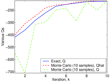
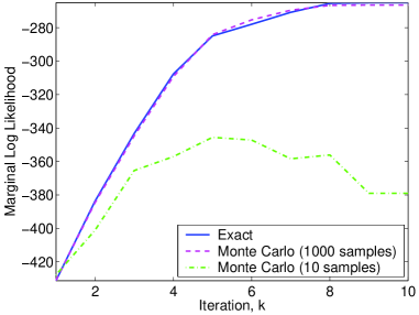
Figure 3: An example with simulated observations illustrating that the Monte Carlo EM algorithm may not result in monotonic increase of the marginal log-likelihood if too few Monte Carlo samples are used. The solid line in (a) is $Q(\mbox{\boldmath$\theta$}^{k+1};\mbox{\boldmath$\theta$}^{k})$ for exact EM iterations, the dashed line is $\widehat{Q}(\widehat{}\mbox{\boldmath$\theta$}^{k+1};\widehat{}\mbox{\boldmath$\theta$}^{k})$ and the dash-dot line is $Q(\widehat{}\mbox{\boldmath$\theta$}^{k+1};\widehat{}\mbox{\boldmath$\theta$}^{k})$ for Monte Carlo EM iterations using only 10 samples. Even though $\widehat{Q}$ increases monotonically, $Q$ may not be monotonic for the Monte Carlo EM algorithm. Figure (b) depicts the marginal log-likelihood for exact EM iterates and for two versions of the Monte Carlo EM. Monte Carlo EM performance closely resembles that of the exact EM algorithm when sufficiently many importance samples are used.

Recently, researchers have considered the question of how many importance samples should be used in a Monte Carlo E-step [3, 5, 11]. The goal is to balance monotonicity and computational efficiency by using enough samples to have a good chance at monotonicity while not using excessively many samples. Booth et al. [3] argue that if the same number of importance samples is used at each EM iteration, then the algorithm will eventually be swamped by Monte Carlo error and will not converge. They also suggest requiring that a convergence criterion be satisfied on multiple successive iterations since the criterion may be met prematurely due to poor Monte Carlo approximations.

Caffo et al. [5] propose a method for automatically adapting the number of Monte Carlo samples used at each EM iteration. To lighten notation, we drop the superscripts $k$ and $k+1$. Let $\Delta(\mbox{\boldmath$\theta$})=Q(\mbox{\boldmath$\theta$};\mbox{\boldmath$\theta$}^{\prime})-Q(\mbox{\boldmath$\theta$}^{\prime};\mbox{\boldmath$\theta$}^{\prime})$ and $\widehat{\Delta}(\mbox{\boldmath$\theta$})=\widehat{Q}(\mbox{\boldmath$\theta$};\mbox{\boldmath$\theta$}^{\prime})-\widehat{Q}(\mbox{\boldmath$\theta$}^{\prime};\mbox{\boldmath$\theta$}^{\prime})$. Furthermore, let $\widehat{}\mbox{\boldmath$\theta$}=\arg\max_{\mbox{\boldmath$\theta$}}\widehat{Q}(\mbox{\boldmath$\theta$};\mbox{\boldmath$\theta$}^{\prime})$, where $\mbox{\boldmath$\theta$}^{\prime}=\mbox{\boldmath$\theta$}^{k}$ was determined at the previous EM iteration. Recall that $L$ importance samples are used to calculate $\widehat{Q}$. The algorithm of Caffo et al. is based on a Central Limit Theorem-like approximation in which they show that $\sqrt{L}\big{(}\widehat{\Delta}(\widehat{}\mbox{\boldmath$\theta$})-\Delta(\widehat{}\mbox{\boldmath$\theta$})\big{)}$ converges in distribution to the standard normal. Observe that the monotonicity property (37) is equivalent to the condition $\Delta(\widehat{}\mbox{\boldmath$\theta$})\geq 0$. Although $\Delta(\widehat{}\mbox{\boldmath$\theta$})$ cannot be computed without computing the exact sufficient statistics $\{\bar{\alpha}_{t^{\prime},t^{\prime\prime}}^{(m)}\}$ and $\{\bar{r}_{1,t^{\prime}}^{(m)}\}$, we can compute $\widehat{\Delta}(\widehat{}\mbox{\boldmath$\theta$})$. Their scheme then amounts to increasing the number of Monte Carlo samples until $\widehat{\Delta}(\widehat{}\mbox{\boldmath$\theta$})>\epsilon$ for a user-specified $\epsilon>0$. Then, applying an asymptotic standard normal tail approximation, they obtain a statement of the form $\Pr\left(\widehat{\Delta}(\widehat{}\mbox{\boldmath$\theta$})-\Delta(\widehat{}\mbox{\boldmath$\theta$})\geq\epsilon\right)\leq\delta(\epsilon)$. Based on this statement they claim that monotonicity holds with probability at least $1-\delta(\epsilon)$. They further remark that if a different $\epsilon_{k}$ is chosen at each iteration, so that $\sum_{k=1}^{\infty}\delta(\epsilon_{k})<\infty$, then, by the Borel-Cantelli Lemma, $\Pr\left(\widehat{\Delta}(\widehat{}\mbox{\boldmath$\theta$})-\Delta(\widehat{}\mbox{\boldmath$\theta$})\geq\epsilon_{k}\ \mbox{i.o.}\right)=0$, so there exists a $K>0$ such that $\widehat{\Delta}(\widehat{}\mbox{\boldmath$\theta$})-\Delta(\widehat{}\mbox{\boldmath$\theta$})<\epsilon_{k}$ for all $k\geq K$ with probability 1; i.e., eventually every EM update is monotonic. Of course, in practice, the algorithm is terminated after a finite number of iterations, so we may never reach the stage where all iterates are monotonic.

Notice that for the monotonicity condition $\Delta(\widehat{}\mbox{\boldmath$\theta$})\geq 0$ to truly hold in the above framework, the events

$$\left\{\widehat{\Delta}(\widehat{}\mbox{\boldmath$\theta$})-\Delta(\widehat{}\mbox{\boldmath$\theta$})\leq\epsilon\right\} \left\{\widehat{\Delta}(\widehat{}\mbox{\boldmath$\theta$})\geq\epsilon\right\}$$ and

must occur simultaneously. Because the probabilistic bound above only addresses one of these events we refer to this type of result as guaranteeing an $(\epsilon,\delta)$-probably approximately monotonic update, or PAM for short. More generally, an $(\epsilon,\delta)$-PAM result states that with probability at least $1-\delta$, the update will be $\epsilon$-approximately monotonic; i.e., $\widehat{\Delta}(\widehat{}\mbox{\boldmath$\theta$})-\Delta(\widehat{}\mbox{\boldmath$\theta$})\leq\epsilon$ implies $\Delta(\widehat{}\mbox{\boldmath$\theta$})\geq-\epsilon$, because, by definition, $\widehat{\Delta}(\widehat{}\mbox{\boldmath$\theta$})\geq 0$.

Rather than resorting to asymptotic approximations to obtain such a result, we can take advantage of the specific form of $Q$ in our problem to obtain the finite-sample PAM result next presented. Recall that independent importance samples are drawn for each co-occurrence observation in the Monte Carlo E-step. Denote by $L_{m}$ the number of importance samples used to compute sufficient statistics for observation ${\bf x}^{(m)}$. Exact E-step computation for this observation requires $N_{m}!$ operations. Similarly, we should expect that larger observations will require more importance samples for two reasons: 1) there are more sufficient statistics associated with this observation ($N_{m}^{2}$ in total), and 2) there are more ways to shuffle these observations.

In the previous section we derived closed form expressions for the importance sample weights, $z_{i}=P[{\bf r}|{\bf x},{\bf A},\mbox{\boldmath$\pi$}]/R[{\bf r}|{\bf x},{\bf A},\mbox{\boldmath$\pi$}]$, where $P$ is the target distribution and $R$ is the importance sampling distribution. A key assumption was made that $P$ is absolutely continuous with respect to $R$; that is, $P[{\bf r}|{\bf x},{\bf A},\mbox{\boldmath$\pi$}]=0$ for every permutation ${\bf r}$ with $R[{\bf r}|{\bf x},{\bf A},\mbox{\boldmath$\pi$}]=0$. We adopt the convention $0/0=0$ so that $z_{i}=0$ for such samples. This guarantees that $z_{i}<\infty$. The bounds below depend on the quality of our importance sample estimators as gauged by

$$b_{m} = \max_{{\bf r}\in\Psi_{N_{m}}}\frac{P[{\bf r}|{\bf x}^{(m)},{\bf A},\mbox{\boldmath$\pi$}]}{R[{\bf r}|{\bf x}^{(m)},{\bf A},\mbox{\boldmath$\pi$}]}.$$ (38)

Because the set $\Psi_{N_{m}}$ is finite, $P$ and $R$ have finite support, and the maximum is well-defined. If $R$ matches the target distribution $P$ well then $b_{m}$ should not be very large.

There is one other subtlety we will account for in our bounds. Because $\widehat{Q}(\mbox{\boldmath$\theta$};\mbox{\boldmath$\theta$}^{\prime})$ has terms $\log A_{i,j}$ and $\log\pi_{i}$, in practice we typically bound $A_{i,j}$ and $\pi_{i}$ away from zero to ensure that $\widehat{Q}$ does not go to $-\infty$. To this end, we will assume that $\widehat{A}_{i,j}\geq\theta_{\min}$ and $\widehat{\pi}_{i}\geq\theta_{\min}$ for some $0<\theta_{\min}<|S|^{-1}$. The upper bound on $\theta_{\min}$ ensures it is still possible to satisfy the constraints (1). Generally we choose $\theta_{\min}$ very close to zero; at machine precision, for example.

We have the following finite-sample PAM result for our Monte Carlo EM algorithm.

Theorem 1.

Let $\epsilon>0$ and $\delta>0$ be given and assume there exists $\theta_{\min}\in(0,|S|^{-1})$ such that $A^{\prime}_{i,j}\geq\theta_{\min}$ and $\pi^{\prime}_{i}\geq\theta_{\min}$ for all $i$ and $j$. If

$$L_{m} = \frac{2T^{2}N_{m}^{4}b_{m}^{2}\ |\log\theta_{\min}|^{2}}{\epsilon^{2}}\log\left(\frac{2N_{m}^{2}}{1-(1-\delta)^{1/T}}\right)$$ (39)

importance samples are used for the $m$th observation then $\widehat{\Delta}(\widehat{}\mbox{\boldmath$\theta$})-\Delta(\widehat{}\mbox{\boldmath$\theta$})<\epsilon$ with probability greater than $1-\delta$.

The proof of Theorem 1 appears in Appendix A. Because $\widehat{\Delta}(\widehat{}\mbox{\boldmath$\theta$})\geq 0$ by definition, the theorem guarantees that $\Delta(\widehat{}\mbox{\boldmath$\theta$})>-\epsilon$ with probability greater than $1-\delta$.

Recall that exact E-step computation requires $N_{m}!$ operations for the $m$th observation. The bound above stipulates that the number of importance samples required is proportional to $N_{m}^{4}\log N_{m}^{2}$, and generating one importance sample requires $N_{m}$ operations. Thus, the computational complexity of a PAM Monte Carlo update only depends on $N_{m}^{5}\log N_{m}^{2}$, which clearly demonstrates that the computational complexity of the Monte Carlo E-step depends polynomially on the $N_{m}$ in comparison to exponential dependence for the exact E-step.

To put this result in perspective, observe that the value of $L_{m}$ given by (39) is roughly a factor of $T$ away from the value we would expect based on an asymptotic variance calculation. Ignoring constants and log terms, for fixed $\theta$ we have

$$\mbox{Var}\left(\widehat{\Delta}(\mbox{\boldmath$\theta$})\right) \approx \mbox{Var}\left(\sum_{m=1}^{T}\sum_{t^{\prime},t^{\prime\prime}=1}^{N_{m}}\widehat{\alpha}_{t^{\prime},t^{\prime\prime}}^{(m)}+\sum_{m=1}^{T}\sum_{t^{\prime}=1}^{N_{m}}\widehat{r}_{1,t^{\prime}}^{(m)}\right)$$

$$= \sum_{m=1}^{T}\mbox{Var}\left(\sum_{t^{\prime},t^{\prime\prime}=1}^{N_{m}}\widehat{\alpha}_{t^{\prime},t^{\prime\prime}}^{(m)}+\sum_{t^{\prime}=1}^{N_{m}}\widehat{r}_{1,t^{\prime}}^{(m)}\right),$$

since independent sets of importance samples are used to calculate sufficient statistics for different observations. It is easily shown that the variance of an individual approximate statistic $\widehat{\alpha}_{t^{\prime},t^{\prime\prime}}^{(m)}$ or $\widehat{r}_{1,t^{\prime}}^{(m)}$ decays according to the parametric rate; i.e., $\mbox{Var}(\widehat{\alpha}_{t^{\prime},t^{\prime\prime}}^{(m)})\simeq 1/L_{m}$. In total, there are $N_{m}^{2}$ sufficient statistics for the $m$th observation, and they are all potentially correlated since they are functions of the same set of importance samples. Then we have

$$\mbox{Var}\left(\widehat{\Delta}(\mbox{\boldmath$\theta$})\right) \approx \sum_{m=1}^{T}\frac{\left(N_{m}^{2}\right)^{2}}{L_{m}}.$$

To drive $\mbox{Var}\left(\widehat{\Delta}(\mbox{\boldmath$\theta$})\right)$ down to a constant level, independent of $T$ and $N_{m}$, we need $L_{m}\propto TN_{m}^{4}$. The additional factor of $T$ in our bound is essentially an artifact from the union bound.

Although the PAM result is pleasing, we would prefer to guarantee monotonicity with high probability, not just approximate monotonicity. Let $\mbox{\boldmath$\theta$}^{*}=\arg\max_{\mbox{\boldmath$\theta$}}Q(\mbox{\boldmath$\theta$};\mbox{\boldmath$\theta$}^{\prime})$. By bounding $\Delta(\widehat{}\mbox{\boldmath$\theta$})-\Delta(\mbox{\boldmath$\theta$}^{*})$ instead of $\widehat{\Delta}(\widehat{}\mbox{\boldmath$\theta$})-\Delta(\widehat{}\mbox{\boldmath$\theta$})$ we obtain the following stronger result guaranteeing monotonicity with high probability. Instead of restricting $A_{i,j}\geq\theta_{\min}$ and $\pi_{i}\geq\theta_{\min}$, we need to assume the variables $\bar{\alpha}_{t^{\prime},t^{\prime\prime}}^{(m)}$ and $\bar{r}_{1,t^{\prime}}^{(m)}$ are bounded away from zero. This is stronger than the previous assumption in the sense that it implies $A_{i,j}$ and $\pi_{i}$ are bounded away from zero.

Theorem 2.

Let $\delta>0$ be given and assume there exists $\lambda>0$ such that $\bar{\alpha}_{t^{\prime},t^{\prime\prime}}^{(m)}>\lambda$ and $\bar{r}_{1,t^{\prime}}^{(m)}>\lambda$, for all $t^{\prime}$ and $t^{\prime\prime}$. If

$$L_{m} = \frac{27b_{m}}{\lambda}\left(\frac{2\sum_{m=1}^{T}N_{m}+\Delta(\mbox{\boldmath$\theta$}^{*})}{\Delta(\mbox{\boldmath$\theta$}^{*})}\right)^{2}\log\left(\frac{4\sum_{m=1}^{T}N_{m}^{2}}{\delta}\right)$$ (40)

importance samples are used for the $m$th observation, then $\Delta(\widehat{}\mbox{\boldmath$\theta$})\geq 0$ with probability at least $1-\delta$.

The proof of Theorem 2 appears in Appendix B. Similar to the PAM bound given in Theorem 2, the computational complexity required for a probably monotonic update also depends polynomially on $N_{m}$.

Note that $L_{m}$ depends on $\Delta(\mbox{\boldmath$\theta$}^{*})$. By definition, $\Delta(\mbox{\boldmath$\theta$}^{*})\geq 0$ at every iteration, and typically $\Delta(\mbox{\boldmath$\theta$}^{*})$ is large at earlier EM iterations and approaches zero as the algorithm converges. This dependence supports the observation of Booth et al. mentioned earlier, that the number of importance samples ought to increase at each iteration.

The main assumption of Theorem 2 is that the sufficient statistics are bounded away from zero at each iteration. We motivate this assumption by observing that if the algorithm is initialized with $\pi_{i}^{0}>0$ and $A_{i,j}^{0}>0$ for all $i,j$ then, recalling the closed form E-step expressions, the sufficient statistics do not vanish in a finite number of EM iterations.

Note that if we use different $\delta_{k}$ at each EM iteration, chosen such that $\sum_{k=1}^{\infty}\delta_{k}<\infty$, then by the Borel-Cantelli Lemma one can argue that $\Pr\big{(}\Delta(\widehat{}\mbox{\boldmath$\theta$})<0\ \mbox{ i.o.}\big{)}=0$. In other words, eventually all EM iterates result in a monotonic increase of the marginal log-likelihood.

In addition to demonstrating that the Monte Carlo EM algorithm has polynomial computational complexity, these bounds give a useful guideline for determining how many importance samples should be used. However, because they involve worst-case analysis, the numbers of samples dictated by these bounds tend to be on the conservative side. For example, in the Internet experiments described in Section 6, $T=249$ and $\bar{N}=17$. Theorem 2 suggests that roughly 72 million importance samples should be used per observation. However, in our experiments we find that the algorithm exhibits reasonable performance on this data set using as few as $2,000$ samples per observation. Of course, in practice, we do not have direct access to the parameters $b_{m}$, $\lambda$, or $\Delta(\mbox{\boldmath$\theta$}^{*})$, so these bounds cannot be used as explicit guidelines.

6 Experimental Results

In this section, we evaluate the performance of our network inference from co-occurrences (NICO) algorithm on simulated data and on data gathered from the public Internet. In the results reported below, network reconstructions are obtained by first estimating an initial state distribution and probability transition matrix via the EM algorithm. Then, we compute the most likely order of each observation according to the inferred model and use this ordering to reconstruct a feasible network. The EM algorithm cannot be guaranteed to converge to a global maximum (the marginal log-likelihood is not concave) and there may even be multiple global maxima. To address this issue, we rerun the EM algorithm from multiple random initializations and report the collective results.

We compare the performance of our algorithm with that of the frequency method (FM), defined in [21] and mentioned in Section 1. The FM also reconstructs a network topology by estimating an order of the vertices in each observation. This method individually determines each path ordering independently by sorting the elements in the path according to a score computed from pair-wise co-occurrence frequencies involving the source and destination of the path. It is possible that multiple vertices may receive identical FM scores, in which case their sorting would be arbitrary (one could exchange elements with identical scores without violating the FM criteria). In fact, we observe this phenomenon in many of our experiments. Ties are resolved by choosing a random order for elements with identical scores. Multiple restarts are also performed using the FM, yielding a collection of feasible solutions.

The quality of a network reconstruction is determined by a quantity we term the edge symmetric difference error. Because the nodes in the network have unique labels, the goal of any reconstruction scheme is to determine which vertices are connected by an edge. The edge symmetric difference error is defined as the sum of the number of false positives (edges appearing in the reconstructed network which do not exist in the true network) and the number of false negatives (edges in the true network not appearing in the reconstructed network).

6.1 Simulated Networks

Our synthetic data is obtained as described next. A network is generated according to a random geometric graph model: 50 vertices are thrown at random in the unit square, and two vertices are connected with an edge if the Euclidean distance between them is less than or equal to $\sqrt{\log(50)/50}$. This threshold guarantees that the graph is connected with high probability. Groups of nodes are randomly chosen as sources and destinations, transmission paths are generated between each source-destination pair according to either a shortest path or random routing model, and then co-occurrence observations are formed from each path. We keep the number of sources fixed at 5 and vary the number of destinations between 5 and 40, to see how the number of observations effects performance. Each experiment is repeated on 100 different topologies, using 10 restarts of both NICO and the FM per configuration. Exact E-step calculation is used for observations with $N_{m}\leq 12$, and causal importance sampling (2000 samples) is used for longer paths. The longest observation in our data was obtained by random routing and has $N_{m}=19$ (notice that $19!\simeq 10^{17}$).

Figure 4 plots edge symmetric difference performance for synthetic data generated using (a) shortest path routing and (b) random routing. The edge symmetric difference error is computed between the inferred network and the graph obtained from correctly ordered observations. Of the 10 solutions corresponding to different NICO initializations, we use the one based on parameter estimates yielding the highest likelihood score. For this simulation, the most likely NICO solution also always resulted in the best edge symmetric difference error.

The FM does not provide a similar mechanism for ranking different solutions. A possible heuristic would be to choose the sparsest solution (with fewest edges). The figures show performance for both this heuristic, and clairvoyantly choosing the best (lowest error) solution of the 10. In fact, using the sparsest solution does better than just choosing a FM solution at random but not as well as using the clairvoyant best. In these simulations, NICO consistently outperform the FM.

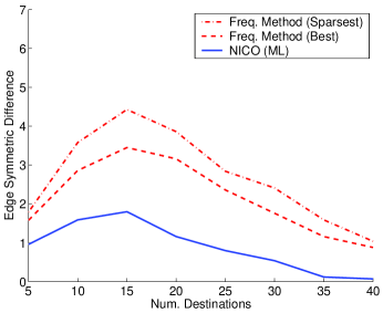
(a) Shortest path routes

(b) Random routes

Figure 4: Edge symmetric differences between inferred networks and the network one would obtain using co-occurrence measurements arranged in the correct order. Performance is averaged over 100 different network configurations. For each configuration 10 NICO and FM solutions are obtained via different initializations. We then choose the NICO solution yielding the largest likelihood, and compare with both the sparsest and clairvoyant best FM solution.

Notice that both algorithms exhibit their worst performance at an intermediate number of destinations. When very few destinations are used the measured topology closely resembles a tree, regardless of the underlying routing mechanism. Relative frequencies of co-occurrence accurately reflect the network distance of each internal vertex from the path endpoints. At the other extreme, when many destinations are used, there is significant overlap among the co-occurrence observations which aids in localizing vertices. In general, the FM seems to be much more sensitive to the amount of data available.

As expected, the FM generally performs better on shortest path data than it does on random routes. When routes are generated randomly the corresponding topology is less tree-like and pair-wise co-occurrence frequencies do not reflect network distances. Because NICO is not based on a particular routing paradigm it performs similarly in both scenarios, possibly even a little better when routing is random.

6.2 Internet Data

We have also studied the performance of our algorithm on co-occurrence observations gathered from the Internet. Using traceroute we have collected data describing roughly 250 router-level paths from sources at the University of Wisconsin-Madison, the Instituto Superior Técnico in Lisbon, and Rice University to 83 servers affiliated with corporations, universities, and governments around the world. Our motivation for using this type of data is two-fold. First, traceroute allows us to measure the true order of elements in each path so that we have a ground truth to validate our results against. Second, and more importantly, the data comes from a real network where, presumably, paths are not generated according to a first-order Markov model. This allows us to gauge the robustness of the proposed model and to evaluate how well it generalizes to realistic scenarios. The ground truth network contains a total of 1105 nodes and 1317 edges, and the longest observed path has length 27.

For this data set we rerun FM and NICO each from 50 random initializations and look at performance across all solutions rather than focusing on the maximum likelihood or clairvoyant best. The exact E-step is used to compute $\bar{\alpha}$ for paths of up to 9 hops. For paths longer than 9 hops, we use the causal importance sampling described in Section 4.1, with 2000 samples per observation.

Minimum, median, and maximum edge symmetric difference errors are shown in Figure 5. Both algorithms have seemingly high error rates, as there are roughly 1300 links in the true network. However keep in mind that both algorithms are attempting to fill in the entries of a roughly $1100\times 1100$ matrix. For 50 networks constructed by choosing a random order for the elements of each observation the average edge symmetric difference error was 4300, so both algorithms are indeed doing considerably better than random guessing. NICO performance is again noticeably better than that of the FM; the NICO average error is better than that of the best FM reconstruction, and the worst case NICO reconstruction is on par with the average FM performance. We also note that the number of false positives and false negatives in a reconstruction using either scheme tend to be roughly equal (each constituting half of the edge symmetric difference error).

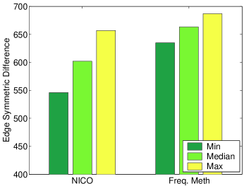
Figure 5: Edge symmetric difference error comparison of NICO and FM on Internet data. The reported values come from 50 random initializations of each algorithm.

Figure 6 shows statistics for the number of edges in the reconstructed networks. There is an interesting correlation between the number of edges and reconstruction accuracy in this example. As seen above, the typical NICO reconstruction is more accurate, in terms of edge errors, than a FM reconstruction. NICO also consistently returns a sparser estimate. The median number of links in a NICO reconstruction is 1329, whereas the median number of links in a FM reconstruction is 1426. There are 1317 edges in the true network, so in this sense the NICO reconstructions more accurately reflect the inherent level of complexity in the true network.

Figure 6: Number of edges in networks reconstructed using each method. The median number of edges per reconstruction is 1329 for NICO and 1426 for FM. The true network has 1317 edges, and so it appears that NICO does a better job of capturing the complexity of the true network.

Marginal log-likelihood values for each of the 50 NICO estimates are depicted in Figure 7. The marginal log-likelihood, given by (4), is the cost function being optimized by the EM algorithm. In contrast to the experiments with simulated data reported above, there is no exact correlation between higher marginal likelihood values and lower edge symmetric difference error for this example. The topology with the highest likelihood value results in an edge symmetric difference error of 627. This is better than the clairvoyant best FM error, but only average for NICO. The three repetitions which returned a topology with the lowest symmetric difference error had the next highest likelihood value, as indicated by the three hollow circles in the figure. The dashed line shows the likelihood value based on a transition matrix estimated using the true path orders as measured by traceroute. Notice that the majority of the NICO solutions have a higher marginal likelihood than the true topology. This suggests that our generative model may not be the best match for Internet topology data. Still the overall performance of our algorithm is encouraging.

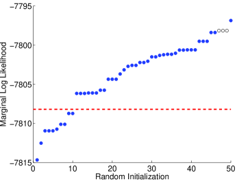
Figure 7: Marginal log likelihood values for different random initializations of NICO, sorted in ascending order. The three hollow circles correspond to the solutions which achieve the lowest edge symmetric difference error of all NICO trials. The red line shows the marginal log likelihood value computed using the true path orders to estimate a Markov transition matrix. Most NICO solutions have higher marginal log-likelihood than the true topology, suggesting that our generative model does not accurately describe Internet topology data.

7 Discussion and Ongoing Research

This paper presents a novel approach to network inference from co-occurrence observations. A co-occurrence observation reflects which vertices are activated by a particular transmission through the network, but not the order in which they are activated. We model transmission paths as a random walks on the underlying graph structure. Co-occurrence observations are modelled as i.i.d. samples of the random walk subjected to a random permutation which accounts for the lack of observed path order. Treating the random permutations as latent variables we derive an expectation-maximization (EM) algorithm for efficiently computing maximum likelihood or maximum a posteriori estimates of the random walk parameters (initial state distribution and transition matrix).

The complexity of the EM algorithm is dominated by the E-step calculation which is exponential in the length of the longest transmission path. In order to handle large networks, we describe fast approximation methods based on importance sampling and Monte Carlo techniques. We derive concentration-style bounds on the accuracy of the Monte Carlo approximation. These bounds prescribe how many importance samples must be used to ensure a monotonic increase in the log-likelihood, thereby guaranteeing convergence of the algorithm with high probability. The resulting Monte Carlo EM computational complexity only depends polynomially on the length of the longest path.

To obtain a network reconstruction, we determine the most likely order for each co-occurrence observation according to the Markov chain parameter estimates, and then insert edges in the graph based on these ordered transmission paths. This procedure always produces a feasible reconstruction. The parameter estimates produced by the EM algorithm may be useful for other tasks such as guiding an expert to alternative reconstructions by assigning likelihoods to different permutations, or predicting unobserved paths through the network as in [12]. One could also analyze properties of an ensemble of solutions obtained by running the EM algorithm from different initializations, and then posit a new set of experiments to be conducted based on this analysis.

The transition matrix parameter $A_{i,j}$ can be interpreted as estimates of the probability that a transmission will be passed from vertex $i$ to $j$, conditioned on the path reaching $i$; that is, $A_{i,j}=P[Z_{k+1}=j|Z_{k}=i]$. In particular, they are not estimates of the probability of a link existing from $i$ to $j$. Since ${\bf A}$ is a stochastic matrix, each row must sum to 1, and so if vertex $i$ is connected to many other nodes then the unit mass is being spread over more entries. We can obtain joint probabilities, $P[Z_{k}=i,Z_{k+1}=j]$, via Bayes theorem,

$$P[Z_{k+1}=j|Z_{k}=i]=\frac{P[Z_{k}=i,Z_{k+1}=j]}{P[Z_{k}=i]},$$

where $P[Z_{k}=i]$ is the stationary distribution of the chain (not necessarily equal to the initial state distribution). These joint probabilities (appropriately scaled versions of the transition matrix entries) more accurately reflect the likelihood of there being an edge from $i$ to $j$, based on our estimates.

Our future work involves extending and generalizing both algorithmic and theoretical aspects of this work. In our experiments we found that our current model leads to reasonable Internet reconstructions, but we feel there is room for improvement. For example, the structure of Internet paths may depend strongly on the destination of the traffic. We are currently investigating models based on “mixtures of random walks” to account for this added level of dependency.

Co-occurrence observations naturally arise from transmission paths in communication network applications and, to a degree, in biological, social, and brain networks as well. However the physical mechanisms driving interactions in the latter three applications may also correspond to more general connected subgraph structures such as trees or directed acyclic graphs. Extending our methods in this fashion is easily accomplished in theory, however the computational complexity may be significantly increased when more general structures are considered.

In this paper we have also restricted our attention to noise-free observations. We are also interested in extending our algorithm to handle the case where observations reflect a soft probability that a given vertex occurred in the path rather than hard, “active” or “not active”, binary observations. This extension is relevant in many applications including the inference of signal transduction networks (in systems biology) where co-occurrence observations are themselves the result of inference procedures run on experimental data.

Appendix A Proof of Theorem 1

There are two main steps in the proof of Theorem 1. First, we derive a concentration inequality for the importance sample approximations, $\widehat{\alpha}_{t^{\prime},t^{\prime\prime}}^{(m)}$ and $\widehat{r}_{1,t^{\prime}}^{(m)}$. Then we use the inequality to construct a bound for $\widehat{\Delta}(\widehat{}\mbox{\boldmath$\theta$})-\Delta(\mbox{\boldmath$\theta$})$.

Recall the expressions (22) and (23) for importance sample approximations calculated in the Monte Carlo E-step. Both are of the general form $\widehat{\mu}_{L}=\frac{\sum_{i=1}^{L}Z({\bf r}^{i})X({\bf r}^{i})}{\sum_{i=1}^{L}Z({\bf r}^{i})}$, where $Z:\Psi_{N}\rightarrow[0,b]$ and $X:\Psi_{N}\rightarrow\{0,1\}$, and they are approximating $\mu=\sum_{{\bf r}\in\Psi_{N}}X({\bf r})P[{\bf r}|{\bf x},{\bf A},\mbox{\boldmath$\pi$}]$. Note that $\mathbb{E}[\widehat{\mu}_{L}]\neq\mu$, so standard concentration results such as Hoeffding’s inequality or McDiarmid’s bounded-differences inequality do not directly apply; e.g., consider the case $L=1$:

$$\mathbb{E}\left[\frac{Z({\bf r}^{1})X({\bf r}^{1})}{Z({\bf r}^{1})}\right] = \sum_{{\bf r}\in\Psi_{N}}X({\bf r})R[{\bf r}|{\bf x},{\bf A},\mbox{\boldmath$\pi$}]$$ (41)

$$\neq \sum_{{\bf r}\in\Psi_{N}}X({\bf r})P[{\bf r}|{\bf x},{\bf A},\mbox{\boldmath$\pi$}].$$ (42)

We can, however, show that $\widehat{\mu}_{L}$ yields an asymptotically consistent estimate of $\mu$. Observe that

$$\mathbb{E}[Z({\bf r}^{i})] = \sum_{{\bf r}\in\Psi_{N}}\frac{P[{\bf r}|{\bf x},{\bf A},\mbox{\boldmath$\pi$}]}{R[{\bf r}|{\bf x},{\bf A},\mbox{\boldmath$\pi$}]}R[{\bf r}|{\bf x},{\bf A},\mbox{\boldmath$\pi$}]$$ (43)

$$= 1,$$ (44)

since $P$ is a probability distribution on $\Psi_{N}$, and

$$\mathbb{E}[Z({\bf r}^{i})X({\bf r}^{i})] = \sum_{{\bf r}\in\Psi_{N}}\frac{P[{\bf r}|{\bf x},{\bf A},\mbox{\boldmath$\pi$}]}{R[{\bf r}|{\bf x},{\bf A},\mbox{\boldmath$\pi$}]}X({\bf r})R[{\bf r}|{\bf x},{\bf A},\mbox{\boldmath$\pi$}]$$ (45)

$$= \sum_{{\bf r}\in\Psi_{N}}X({\bf r})P[{\bf r}|{\bf x},{\bf A},\mbox{\boldmath$\pi$}]$$ (46)

$$= \mu.$$ (47)

It follows from the strong law of large numbers that $\widehat{\mu}_{L}\rightarrow\mu$ as $L\rightarrow\infty$.

The following finite-sample concentration inequality demonstrates that the approximation error, $\widehat{\mu}_{N}-\mu$, decays exponentially in the number of importance samples, $L$.

Proposition 1.

Let $\{(X_{i},Z_{i})\}$ be a sequence of independent and identically distributed random variables with $X_{i}\in\{0,1\}$ and $Z_{i}\in[0,b]$. Assume that $\mathbb{E}[Z_{i}]=1$ and $\mathbb{E}[Z_{i}X_{i}]=\mu$, and set $\widehat{\mu}_{L}=\frac{\sum_{i=1}^{L}Z_{i}X_{i}}{\sum_{i=1}^{L}Z_{i}}$. Then with probability greater than $1-\delta$,

$$\widehat{\mu}_{L}-\mu < \sqrt{\frac{2b^{2}\log\frac{2}{\delta}}{L}}.$$ (48)

Proof.

From the definitions of $Z_{i}$ and $X_{i}$, $Z_{i}X_{i}\in[0,b]$. Applying Hoeffding’s inequality [10] yields that for any $t>0$,

$$\Pr\left(\sum_{i=1}^{L}Z_{i}X_{i}-L\mu\geq Lt\right) \leq e^{-2Lt^{2}/b^{2}},$$ (49)

and for any $t>0$,

$$\Pr\left(\sum_{i=1}^{L}Z_{i}-L\leq-Lt\right) \leq e^{-2Lt^{2}/b^{2}}.$$ (50)

Define the event, $E_{t}=\left\{\sum_{i=1}^{L}Z_{i}X_{i}-L\mu\geq Lt\right\}\bigcup\left\{\sum_{i=1}^{L}Z_{i}-L\leq-Lt\right\}$. By the union bound, $\Pr(E_{t})\leq 2e^{-2Lt^{2}/b^{2}}$ for any $t>0$. The complement of $E_{t}$ implies that for $t\in(0,1)$,

$$\widehat{\mu}_{L}-\mu = \frac{\sum_{i=1}^{L}Z_{i}X_{i}-L\mu}{\sum_{i=1}^{L}Z_{i}}+\frac{L\mu}{\sum_{i=1}^{L}Z_{i}}-\mu$$ (51)

$$< \frac{Lt}{L(1-t)}+\frac{L\mu}{L(1-t)}-\mu$$ (52)

$$= \frac{t(1+\mu)}{1-t}.$$ (53)

It follows that $\left\{\widehat{\mu}_{L}-\mu\geq\frac{t(1+\mu)}{1-t}\right\}\subseteq E_{t}$, and so $\Pr\left(\widehat{\mu}_{L}-\mu\geq\frac{t(1+\mu)}{1-t}\right)\leq\Pr(E_{t})\leq 2e^{-2Lt^{2}/b^{2}}$. Since $\widehat{\mu}_{L}\leq 1$, if $\frac{t(1+\mu)}{1-t}+\mu>1$ then $\Pr\left(\widehat{\mu}_{L}-\mu\geq\frac{t(1+\mu)}{1-t}\right)=0$, and the proposition holds trivially. Thus, without loss of generality we consider the case $\frac{t(1+\mu)}{1-t}+\mu\leq 1$, or equivalently, $t\leq(1-\mu)/2$. This restriction on $t$ implies $\frac{t(1+\mu)}{1-t}\leq 2t$, and so we have $\Pr\left(\widehat{\mu}_{L}-\mu<2t\right)>1-2e^{-2Lt^{2}/b^{2}}$. Set $\delta=2e^{-2Lt^{2}/b^{2}}$ to obtain the desired result. ∎

We apply Proposition 1 to the Monte Carlo approximations $\{\widehat{\alpha}_{t^{\prime},t^{\prime\prime}}^{(m)}\}$ and $\{\widehat{r}_{1,t^{\prime}}^{(m)}\}$ as follows. Recall that the Monte Carlo weights are bounded according to $z_{i}\in[0,b_{m}]$, with $b_{m}$ as defined in (38). Define

$$B_{\delta^{\prime},L_{m}}^{m} = \left(\bigcup_{\genfrac{}{}{0.0pt}{3}{t^{\prime},t^{\prime\prime}=1}{t^{\prime}\neq t^{\prime\prime}}}^{N_{m}}\left\{\widehat{\alpha}_{t^{\prime},t^{\prime\prime}}^{(m)}-\bar{\alpha}_{t^{\prime},t^{\prime\prime}}^{(m)}\geq\sqrt{\frac{2b_{m}^{2}\log\frac{2}{\delta^{\prime}}}{L_{m}}}\right\}\right)\bigcup\left(\bigcup_{t^{\prime}=1}^{N_{m}}\left\{\widehat{r}_{1,t^{\prime}}^{(m)}-\bar{r}_{1,t^{\prime}}^{(m)}\geq\sqrt{\frac{2b_{m}^{2}\log\frac{2}{\delta^{\prime}}}{L_{m}}}\right\}\right).$$

This is a union over $2\binom{N_{m}}{2}+N_{m}=N_{m}^{2}$ events, each of which holds with probability at most $\delta^{\prime}$ according to Proposition 1. By the union bound it follows that $\Pr(B_{\delta^{\prime},L_{m}}^{m})\leq N_{m}^{2}\delta^{\prime}$. Next, define

$$C_{\delta^{\prime},L_{m}}^{m}=\left\{\sum_{t^{\prime},t^{\prime\prime}=1}^{N_{m}}\left(\widehat{\alpha}_{t^{\prime},t^{\prime\prime}}^{(m)}-\bar{\alpha}_{t^{\prime},t^{\prime\prime}}^{(m)}\right)+\sum_{t^{\prime}=1}^{N_{m}}\left(\widehat{r}_{1,t^{\prime}}^{(m)}-\bar{r}_{1,t^{\prime}}^{(m)}\right)\geq N_{m}^{2}\sqrt{\frac{2b_{m}^{2}\log\frac{2}{\delta^{\prime}}}{L_{m}}}\right\},$$ (54)

and observe that $C_{\delta^{\prime},L_{m}}^{m}\subseteq B_{\delta^{\prime},L_{m}}^{m}$, therefore $\Pr(C_{\delta^{\prime},L_{m}}^{m})\leq\Pr(B_{\delta^{\prime},L_{m}}^{m})\leq N_{m}^{2}\delta^{\prime}$. Let $\delta^{\prime\prime}=N_{m}^{2}\delta^{\prime}$ and let $L>0$ be a value to be determined later. For each $m=1,\dots,T$, set

$$L_{m} = \frac{2LN_{m}^{4}b_{m}^{2}\log\frac{2N_{m}^{2}}{\delta^{\prime\prime}}}{\log\frac{1}{\delta^{\prime\prime}}},$$ (55)

so that

$$N_{m}^{2}\sqrt{\frac{2b_{m}^{2}\log\frac{2}{\delta^{\prime}}}{L_{m}}}\ =\ N_{m}^{2}\sqrt{\frac{2b_{m}^{2}\log\frac{2N_{m}^{2}}{\delta^{\prime\prime}}}{L_{m}}}\ =\ \sqrt{\frac{\log\frac{1}{\delta^{\prime\prime}}}{L}}.$$ (56)

Then with probability greater than $1-\delta^{\prime\prime}$,

$$\sum_{t^{\prime},t^{\prime\prime}=1}^{N_{m}}\left(\widehat{\alpha}_{t^{\prime},t^{\prime\prime}}^{(m)}-\bar{\alpha}_{t^{\prime},t^{\prime\prime}}^{(m)}\right)+\sum_{t^{\prime}=1}^{N_{m}}\left(\widehat{r}_{1,t^{\prime}}^{(m)}-\bar{r}_{1,t^{\prime}}^{(m)}\right) < \sqrt{\frac{\log\frac{1}{\delta^{\prime\prime}}}{L}}.$$ (57)

Recall that $x_{t^{\prime},i}^{(m)}$ are indicator variables satisfying $\sum_{i,j=1}^{|S|}x_{t^{\prime\prime},i}^{(m)}x_{t^{\prime},j}^{(m)}=1$ and $\sum_{i=1}^{|S|}x_{t^{\prime},i}^{(m)}=1$. Multiplying each term in (57) by the appropriate sum of indicators, rearranging terms, and recalling that importance sample estimates for different observations are statistically independent, we have that with probability greater than $(1-\delta^{\prime\prime})^{T}$,

$$\bigcap_{m=1}^{T}\left\{\sum_{t^{\prime},t^{\prime\prime}=1}^{N_{m}}\sum_{i,j=1}^{|S|}\left(\widehat{\alpha}_{t^{\prime},t^{\prime\prime}}^{(m)}-\bar{\alpha}_{t^{\prime},t^{\prime\prime}}^{(m)}\right)x_{t^{\prime\prime},i}^{(m)}x_{t^{\prime},j}^{(m)}+\sum_{t^{\prime}=1}^{N_{m}}\sum_{i=1}^{|S|}\left(\widehat{r}_{1,t^{\prime}}^{(m)}-\bar{r}_{1,t^{\prime}}^{(m)}\right)x_{t^{\prime},i}^{(m)}<\sqrt{\frac{\log\frac{1}{\delta^{\prime\prime}}}{L}}\right\},$$ (58)

which implies that with probability greater than $(1-\delta^{\prime\prime})^{T}$,

$$\sum_{m=1}^{T}\sum_{t^{\prime},t^{\prime\prime}=1}^{N_{m}}\sum_{i,j=1}^{|S|}\left(\widehat{\alpha}_{t^{\prime},t^{\prime\prime}}^{(m)}-\bar{\alpha}_{t^{\prime},t^{\prime\prime}}^{(m)}\right)x_{t^{\prime\prime},i}^{(m)}x_{t^{\prime},j}^{(m)}+\sum_{m=1}^{T}\sum_{t^{\prime}=1}^{N_{m}}\sum_{i=1}^{|S|}\left(\widehat{r}_{1,t^{\prime}}^{(m)}-\bar{r}_{1,t^{\prime}}^{(m)}\right)x_{t^{\prime},i}^{(m)} < T\sqrt{\frac{\log\frac{1}{\delta^{\prime\prime}}}{L}}.$$ (59)

Finally, set $1-\delta=(1-\delta^{\prime\prime})^{T}$ and multiply through by $|\log\theta_{\min}|>0$. Then with probability greater than $1-\delta$,

$$\sum_{m=1}^{T}\sum_{t^{\prime},t^{\prime\prime}=1}^{N_{m}}\sum_{i,j=1}^{|S|}\left(\widehat{\alpha}_{t^{\prime},t^{\prime\prime}}^{(m)}-\bar{\alpha}_{t^{\prime},t^{\prime\prime}}^{(m)}\right)x_{t^{\prime\prime},i}^{(m)}x_{t^{\prime},j}^{(m)}\ |\log\theta_{\min}|+\sum_{m=1}^{T}\sum_{t^{\prime}=1}^{N_{m}}\sum_{i=1}^{|S|}\left(\widehat{r}_{1,t^{\prime}}^{(m)}-\bar{r}_{1,t^{\prime}}^{(m)}\right)x_{t^{\prime},i}^{(m)}\ |\log\theta_{\min}|$$ (60)

$$< T\ |\log\theta_{\min}|\sqrt{\frac{-\log\big{(}1-(1-\delta)^{1/T}\big{)}}{L}}.\hskip 234.87749pt$$

To complete the proof, observe that

$$\widehat{\Delta}(\widehat{}\mbox{\boldmath$\theta$})-\Delta(\widehat{}\mbox{\boldmath$\theta$}) = \sum_{m=1}^{T}\sum_{i,j=1}^{|S|}\sum_{t^{\prime},t^{\prime\prime}}^{N_{m}}\left(\widehat{\alpha}_{t^{\prime},t^{\prime\prime}}^{(m)}-\bar{\alpha}_{t^{\prime},t^{\prime\prime}}^{(m)}\right)x_{t^{\prime\prime},i}^{(m)}x_{t^{\prime},j}^{(m)}\left(\log\widehat{A}_{i,j}-\log A^{\prime}_{i,j}\right)$$ (61)

$$+\sum_{m=1}^{T}\sum_{i=1}^{|S|}\sum_{t^{\prime}=1}^{N_{m}}\left(\widehat{r}_{1,t^{\prime}}^{(m)}-\bar{r}_{1,t^{\prime}}^{(m)}\right)x_{t^{\prime},i}^{(m)}\left(\log\widehat{\pi}_{i}-\log\pi^{\prime}_{i}\right).$$

By assumption, $\theta_{\min}\leq\widehat{A}_{i,j},A^{\prime}_{i,j}\leq 1$ for each $(i,j)\in S^{2}$. It follows that

$$\log\widehat{A}_{i,j}-\log A^{\prime}_{i,j} \leq -\log\theta_{\min}\ =\ |\log\theta_{\min}|.$$ (62)

Similarly, $\log\widehat{\pi}_{i}-\log\pi^{\prime}_{i}\leq|\log\theta_{\min}|$ for each $i\in S$. Apply these bounds in (61) to find that the right hand side of (61) is no greater than the left hand side of (60). Set

$$\epsilon = T\ |\log\theta_{\min}|\sqrt{\frac{\log\frac{1}{1-(1-\delta)^{1/T}}}{L}}.$$ (63)

Then $\widehat{\Delta}(\widehat{}\mbox{\boldmath$\theta$})-\Delta(\widehat{}\mbox{\boldmath$\theta$})<\epsilon$ with probability greater than $1-\delta$. Solve for $L$ in (63) and plug the resulting value back into (55) with $\delta^{\prime\prime}=1-(1-\delta)^{1/T}$ to obtain the desired result.

Appendix B Proof of Theorem 2

To prove Theorem 2 we will show that $\Delta(\widehat{}\mbox{\boldmath$\theta$})>(1-\epsilon)\;\Delta(\mbox{\boldmath$\theta$}^{*})$ with high probability, but first we need two preliminary results. We begin by deriving concentration inequalities for the Monte Carlo sufficient statistics. Then we use these bounds to show that the corresponding M-step parameter estimates, $\widehat{A}_{i,j}$ and $\widehat{\pi}_{i}$ concentrate about their asymptotic means, $A^{*}_{i,j}$ and $\pi^{*}_{i}$. From there we construct the desired bound for $\Delta(\widehat{}\mbox{\boldmath$\theta$})$, which implies the theorem since $\Delta(\mbox{\boldmath$\theta$}^{*})\geq 0$ by definition.

The proof of Theorem 1 makes use of additive concentration inequalities, bounding the probability of deviations of the form $\widehat{\mu}_{L}-\mu\geq t$. In this proof we make use of relative concentration inequalities to ensure that $\widehat{\mu}_{L}>(1+\epsilon)\mu$ with high probability.

Proposition 2.

Let $\{(X_{i},Z_{i})\}$ be a sequence of independent and identically distributed random variables with $X_{i}\in\{0,1\}$ and $Z_{i}\in[0,b]$. Assume that $\mathbb{E}[Z_{i}]=1$ and $\mathbb{E}[Z_{i}X_{i}]=\mu$, and set $\widehat{\mu}_{L}=\frac{\sum_{i=1}^{L}Z_{i}X_{i}}{\sum_{i=1}^{L}Z_{i}}$, as before. Then with probability greater than $1-\delta$,

$$\widehat{\mu}_{L} < \left(1+\sqrt{\frac{27b\log\frac{2}{\delta}}{L\mu}}\right)\mu,$$

and with probability greater than $1-\delta$,

$$\widehat{\mu}_{L} > \left(1-\sqrt{\frac{27b\log\frac{2}{\delta}}{L\mu}}\right)\mu.$$

Proof.

Since $X_{i}\in\{0,1\}$ and $Z_{i}\in[0,b]$, $Z_{i}X_{i}\in[0,b]$ also. Applying the relative form of Hoeffding’s inequality (see, e.g., Theorem 2.3 in [17]), we have that for any $\beta>0$,

$$\Pr\left(\sum_{i=1}^{L}Z_{i}X_{i}\geq(1+\beta)L\mu\right) \leq \exp\left\{\frac{-L\mu\beta^{2}}{2b(1+\beta/3)}\right\}.$$ (64)

If $\beta\leq 1$ then $2(1+\beta/3)<3$, and so for $\beta\in(0,1]$,

$$\Pr\left(\sum_{i=1}^{L}Z_{i}X_{i}\geq(1+\beta)L\mu\right) \leq \exp\left\{\frac{-L\mu\beta^{2}}{3b}\right\},$$ (65)

which suffices for our application. Also, for any $\gamma>0$,

$$\Pr\left(\sum_{i=1}^{L}Z_{i}\leq(1-\gamma)L\right) \leq \exp\left\{\frac{-L\gamma^{2}}{2b}\right\}.$$ (66)

Suppose the events

$$\left\{\sum_{i=1}^{L}Z_{i}X_{i}<(1+\beta)L\mu\right\} \left\{\sum_{i=1}^{L}Z_{i}>(1-\gamma)L\right\}$$ and (67)

occur simultaneously. Then for $0<\gamma<1$,

$$\widehat{\mu}_{L} > \left(\frac{1+\beta}{1-\gamma}\right)\mu.$$ (68)

Since we will apply the union bound, we balance the exponential rates in (65) and (66) by setting $\gamma=\beta\sqrt{\frac{2}{3}\mu}<1$. Solving

$$\frac{1+\beta}{1-\gamma}=\frac{1+\beta}{1-\beta\sqrt{\frac{2}{3}\mu}}=1+\epsilon$$ (69)

for $\beta$ in terms of $\epsilon$ leads to

$$\beta = \frac{\epsilon}{1+\sqrt{\frac{2}{3}\mu}+\epsilon\sqrt{\frac{2}{3}\mu}}.$$ (70)

In order to ensure that $\beta\leq 1$ we restrict

$$\epsilon \leq \frac{1+1}{1-\sqrt{\frac{2}{3}\mu}}-1$$ (71)

$$= \frac{1+\sqrt{\frac{2}{3}\mu}}{1-\sqrt{\frac{2}{3}\mu}}.$$ (72)

Note that the right hand side of the expression above is at least 1 for all $\mu\in[0,1]$. Apply the union bound with the complements of the events in (67) using (70) in the exponent, and observe that $1+\sqrt{\frac{2}{3}\mu}+\epsilon\sqrt{\frac{2}{3}\mu}\leq 3$ for all $\mu\in[0,1]$ and $\epsilon\in(0,1)$ to find that $\Pr\left(\widehat{\mu}_{L}\leq(1+\epsilon)\mu\right)\leq 2e^{-L\mu\epsilon^{2}/27b^{2}}$. Set $\delta=2e^{-L\mu\epsilon^{2}/27b^{2}}$ to obtain the first claim. The proof of the second claim follows a similar sequence of steps. See [20] for the full details. ∎

Application of the union bound yields the following.

Corollary 1.

With probability greater than $1-\delta$,

$$\left(1-\sqrt{\frac{27b\log\frac{4}{\delta}}{L\mu}}\right)\mu\ <\ \widehat{\mu}_{L}\ <\ \left(1+\sqrt{\frac{27b\log\frac{4}{\delta}}{L\mu}}\right)\mu.$$ (73)

Next we apply Corollary 1 to the Monte Carlo approximations, $\{\widehat{r}_{1,t^{\prime}}^{(m)}\}$ and $\{\widehat{\alpha}_{t^{\prime},t^{\prime\prime}}^{(m)}\}$ towards showing that $\widehat{A}_{i,j}$ and $\widehat{\pi}_{i}$ do not deviate too greatly from $A_{i,j}^{*}$ and $\pi_{i}^{*}$. Recall the exact M-step expressions for $\pi^{*}_{i}$ and $A^{*}_{i,j}$ given by (18). The corresponding expressions for $\widehat{\pi}_{i}$ and $\widehat{A}_{i,j}$ are found by replacing each $\bar{r}_{1,t^{\prime}}^{(m)}$ and $\bar{\alpha}_{t^{\prime},t^{\prime\prime}}^{(m)}$ with $\widehat{r}_{1,t^{\prime}}^{(m)}$ and $\widehat{\alpha}_{t^{\prime},t^{\prime\prime}}^{(m)}$. By appropriately bounding the numerators and denominators of $\widehat{A}_{i,j}$ and $\widehat{\pi}_{i}$ we obtain the following result.

Proposition 3.

Let $L>0$ and $\delta>0$ be given. Assume that there exists $\lambda>0$ such that $\bar{r}_{1,t^{\prime}}^{(m)}\geq\lambda$ and $\bar{\alpha}_{t^{\prime},t^{\prime\prime}}^{(m)}\geq\lambda$ for all $m=1,\dots,T$ and $t^{\prime},t^{\prime\prime}=1,\dots,N_{m}$. If at least $L_{m}\geq\frac{27b_{m}L}{\lambda}$ importance samples are used, then with probability at least $1-(\sum_{m=1}^{T}N_{m}^{2})\delta$,

$$\left(\bigcap_{i,j=1}^{|S|}\left\{\widehat{A}_{i,j}>\left(\frac{1-\sqrt{\frac{\log\frac{4}{\delta}}{L}}}{1+\sqrt{\frac{\log\frac{4}{\delta}}{L}}}\right)A^{*}_{i,j}\right\}\right)\bigcap\left(\bigcap_{i=1}^{|S|}\left\{\widehat{\pi}_{i}>\left(\frac{1-\sqrt{\frac{\log\frac{4}{\delta}}{L}}}{1+\sqrt{\frac{\log\frac{4}{\delta}}{L}}}\right)\pi^{*}_{i}\right\}\right).$$ (74)

Proof.

First recall that there are $2\binom{N_{m}}{2}+N_{m}=N_{m}^{2}$ sufficient statistics associated with the $m$th observation: one $\alpha_{t^{\prime},t^{\prime\prime}}^{(m)}$ for each of the $2\binom{N_{m}}{2}$ possible transitions and one $r_{1,t^{\prime}}^{(m)}$ for each possible initial state. Then, in total there are $\sum_{m=1}^{T}N_{m}^{2}$ sufficient statistics to calculate in the E-step. Applying the union bound in conjunction with (73) we have that with probability greater than $1-(\sum_{m=1}^{T}N_{m}^{2})\delta$,

$$\bar{\alpha}_{t^{\prime},t^{\prime\prime}}^{(m)}-\sqrt{\frac{27b_{m}\bar{\alpha}_{t^{\prime},t^{\prime\prime}}^{(m)}\log\frac{4}{\delta}}{L_{m}}}\ <\ \widehat{\alpha}_{t^{\prime},t^{\prime\prime}}^{(m)}\ <\ \bar{\alpha}_{t^{\prime},t^{\prime\prime}}^{(m)}+\sqrt{\frac{27b_{m}\bar{\alpha}_{t^{\prime},t^{\prime\prime}}^{(m)}\log\frac{4}{\delta}}{L_{m}}},$$ (75)

for all $m=1,\dots,T$ and $t^{\prime},t^{\prime\prime}=1,\dots,N_{m}$, and

$$\bar{r}_{1,t^{\prime}}^{(m)}-\sqrt{\frac{27b_{m}\bar{r}_{1,t^{\prime}}^{(m)}\log\frac{4}{\delta}}{L_{m}}}\ <\ \widehat{r}_{1,t^{\prime}}^{(m)}\ <\ \bar{r}_{1,t^{\prime}}^{(m)}+\sqrt{\frac{27b_{m}\bar{r}_{1,t^{\prime}}^{(m)}\log\frac{4}{\delta}}{L_{m}}},$$ (76)

for all $m=1,\dots,T$ and $t^{\prime}=1,\dots,N_{m}$. Based on the assumption that $\bar{\alpha}_{t^{\prime},t^{\prime\prime}}^{(m)}\geq\lambda$ and $\bar{r}_{1,t^{\prime}}^{(m)}\geq\lambda$, taking $L_{m}\geq 27b_{m}L/\lambda$ guarantees that

$$L_{m} \geq \max\left(\max_{t^{\prime},t^{\prime\prime}=1,\dots,N_{m}}\frac{27b_{m}L}{\bar{\alpha}_{t^{\prime},t^{\prime\prime}}^{(m)}};\ \max_{t^{\prime}=1,\dots,N_{m}}\frac{27b_{m}L}{\bar{r}_{1,t^{\prime}}^{(m)}}\right).$$ (77)

Then with probability greater than $1-(\sum_{m=1}^{T}N_{m}^{2})\delta$,

$$\left(1-\sqrt{\frac{\log\frac{4}{\delta}}{L}}\right)\bar{\alpha}_{t^{\prime},t^{\prime\prime}}^{(m)}\ <\ \widehat{\alpha}_{t^{\prime},t^{\prime\prime}}^{(m)}\ <\ \left(1+\sqrt{\frac{\log\frac{4}{\delta}}{L}}\right)\bar{\alpha}_{t^{\prime},t^{\prime\prime}}^{(m)},$$ (78)

for all $m=1,\dots,T$ and $t^{\prime},t^{\prime\prime}=1,\dots,N_{m}$, and

$$\left(1-\sqrt{\frac{\log\frac{4}{\delta}}{L}}\right)\bar{r}_{1,t^{\prime}}^{(m)}\ <\ \widehat{r}_{1,t^{\prime}}^{(m)}\ <\ \left(1+\sqrt{\frac{\log\frac{4}{\delta}}{L}}\right)\bar{r}_{1,t^{\prime}}^{(m)},$$ (79)

for all $m=1,\dots,T$ and $t^{\prime}=1,\dots,N_{m}$.

Equation (78) implies that for each $(i,j)\in S^{2}$,

$$\sum_{m=1}^{T}\sum_{t^{\prime},t^{\prime\prime}=1}^{N_{m}}\widehat{\alpha}_{t^{\prime},t^{\prime\prime}}^{(m)}x_{t^{\prime\prime},i}^{(m)}x_{t^{\prime},j}^{(m)} > \left(1-\sqrt{\frac{\log\frac{4}{\delta}}{L}}\right)\sum_{m=1}^{T}\sum_{t^{\prime},t^{\prime\prime}=1}^{N_{m}}\bar{\alpha}_{t^{\prime},t^{\prime\prime}}^{(m)}x_{t^{\prime\prime},i}^{(m)}x_{t^{\prime},j}^{(m)},$$

and for each $i\in S$,

$$\sum_{k=1}^{|S|}\sum_{m=1}^{T}\sum_{t^{\prime},t^{\prime\prime}}^{(m)}\widehat{\alpha}_{t^{\prime},t^{\prime\prime}}^{(m)}x_{t^{\prime\prime},i}^{(m)}x_{t^{\prime},k}^{(m)} < \left(1+\sqrt{\frac{\log\frac{4}{\delta}}{L}}\right)\sum_{k=1}^{|S|}\sum_{m=1}^{T}\sum_{t^{\prime},t^{\prime\prime}=1}^{N_{m}}\bar{\alpha}_{t^{\prime},t^{\prime\prime}}^{(m)}x_{t^{\prime\prime},i}^{(m)}x_{t^{\prime},k}^{(m)}.$$

Taking the ratio of these two expressions yields the desired result for $\widehat{A}_{i,j}$ and $A^{*}_{i,j}$.

Similarly, (79) implies that for each $i$,

$$\sum_{m=1}^{T}\sum_{t^{\prime}=1}^{N_{m}}\widehat{r}_{1,t^{\prime}}^{(m)}x_{t^{\prime},i}^{(m)} > \left(1-\sqrt{\frac{\log\frac{4}{\delta}}{L}}\right)\sum_{m=1}^{T}\sum_{t^{\prime}}^{N_{m}}\bar{r}_{1,t^{\prime}}^{(m)}x_{t^{\prime},i}^{(m)},$$ (80)

and for each $i$,

$$\sum_{m=1}^{T}\sum_{t^{\prime}=1}^{N_{m}}\widehat{r}_{1,t^{\prime}}^{(m)}x_{t^{\prime},i}^{(m)} < \left(1+\sqrt{\frac{\log\frac{4}{\delta}}{L}}\right)\sum_{m=1}^{T}\sum_{t^{\prime}}^{N_{m}}\bar{r}_{1,t^{\prime}}^{(m)}x_{t^{\prime},i}^{(m)}.$$ (81)

Taking the ratio of these two expressions yields the desired result for $\widehat{\pi}_{i}$ and $\pi^{*}_{i}$. ∎

The remainder of the proof of Theorem 2 is now fairly straightforward. Let $\delta>0$ be the value given in the statement of Theorem 2. Monotonicity of the logarithm in conjunction with Proposition 3 implies that with probability greater than $1-\delta$, for all $i,j\in S$,

$$\log\widehat{A}_{i,j} > \log A^{*}_{i,j}+\log\left(\frac{1-\sqrt{\frac{\log 4\sum_{m=1}^{T}N_{m}^{2}-\log\delta}{L}}}{1+\sqrt{\frac{\log 4\sum_{m=1}^{T}N_{m}^{2}-\log\delta}{L}}}\right),$$ (82)

$$\log\widehat{\pi}_{i} > \log\pi^{*}_{i}+\log\left(\frac{1-\sqrt{\frac{\log 4\sum_{m=1}^{T}N_{m}^{2}-\log\delta}{L}}}{1+\sqrt{\frac{\log 4\sum_{m=1}^{T}N_{m}^{2}-\log\delta}{L}}}\right).$$ (83)

Multiply through by either $\sum_{m=1}^{T}\sum_{t^{\prime},t^{\prime\prime}=1}^{N_{m}}\bar{\alpha}_{t^{\prime},t^{\prime\prime}}^{(m)}x_{t^{\prime\prime},i}^{(m)}x_{t^{\prime},j}^{(m)}>0$ or $\sum_{m=1}^{T}\sum_{t^{\prime}=1}^{N_{m}}\bar{\alpha}_{t^{\prime},t^{\prime\prime}}^{(m)}x_{t^{\prime},i}^{(m)}>0$ as appropriate, and sum over $i$ and $j$ to obtain

$$\begin{array}[]{l}Q(\widehat{}\mbox{\boldmath$\theta$};\mbox{\boldmath$\theta$}^{\prime})\ >\ Q(\mbox{\boldmath$\theta$}^{*};\mbox{\boldmath$\theta$}^{\prime})\\ \hskip 28.90755pt+\left(\displaystyle\sum_{i,j=1}^{|S|}\sum_{m=1}^{T}\sum_{t^{\prime},t^{\prime\prime}=1}^{N_{m}}\bar{\alpha}_{t^{\prime},t^{\prime\prime}}^{(m)}x_{t^{\prime\prime},i}^{(m)}x_{t^{\prime},j}^{(m)}+\sum_{i=1}^{|S|}\sum_{m=1}^{T}\sum_{t^{\prime}=1}^{N_{m}}\bar{r}_{1,t^{\prime}}^{(m)}x_{t^{\prime},i}^{(m)}\right)\log\left(\frac{1-\sqrt{\frac{\log 4\sum_{m=1}^{T}N_{m}^{2}-\log\delta}{L}}}{1+\sqrt{\frac{\log 4\sum_{m=1}^{T}N_{m}^{2}-\log\delta}{L}}}\right).\end{array}$$ (84)

By the definitions of $x_{t^{\prime},i}^{(m)}$, $\bar{r}_{1,t^{\prime}}^{(m)}$, and $\bar{\alpha}_{t^{\prime},t^{\prime\prime}}^{(m)}$ given in Section 3 we have $\sum_{t^{\prime}=1}^{N_{m}}\bar{r}_{1,t^{\prime}}^{(m)}=1$, $\sum_{t^{\prime},t^{\prime\prime}=1}^{N_{m}}\bar{\alpha}_{t^{\prime},t^{\prime\prime}}^{(m)}=N_{m}-1$, $\sum_{i,j=1}^{|S|}x_{t^{\prime\prime},i}^{(m)}x_{t^{\prime},j}^{(m)}=1$, and $\sum_{i=1}^{|S|}x_{t^{\prime},i}^{(m)}=1$. It follows that

$$\sum_{i,j=1}^{|S|}\sum_{m=1}^{T}\sum_{t^{\prime},t^{\prime\prime}=1}^{N_{m}}\bar{\alpha}_{t^{\prime},t^{\prime\prime}}^{(m)}x_{t^{\prime\prime},i}^{(m)}x_{t^{\prime},j}^{(m)}+\sum_{i=1}^{|S|}\sum_{m=1}^{T}\sum_{t^{\prime}=1}^{N_{m}}\bar{r}_{1,t^{\prime}}^{(m)}x_{t^{\prime},i}^{(m)} = \sum_{m=1}^{T}N_{m}.$$ (85)

Subtract $Q(\mbox{\boldmath$\theta$}^{\prime};\mbox{\boldmath$\theta$}^{\prime})$ from both sides of (84) to obtain that with probability greater than $1-\delta$,

$$\Delta(\widehat{}\mbox{\boldmath$\theta$}) > \Delta(\mbox{\boldmath$\theta$}^{*})+\left(\sum_{m=1}^{T}N_{m}\right)\log\left(\frac{1-\sqrt{\frac{\log 4\sum_{m=1}^{T}N_{m}^{2}-\log\delta}{L}}}{1+\sqrt{\frac{\log 4\sum_{m=1}^{T}N_{m}^{2}-\log\delta}{L}}}\right).$$ (86)

Let $\epsilon>0$ be the value given in the statement of Theorem 2 and set

$$\left(\sum_{m=1}^{T}N_{m}\right)\log\left(\frac{1-\sqrt{\frac{\log 4\sum_{m=1}^{T}N_{m}^{2}-\log\delta}{L}}}{1+\sqrt{\frac{\log 4\sum_{m=1}^{T}N_{m}^{2}-\log\delta}{L}}}\right) = -\epsilon\Delta(\mbox{\boldmath$\theta$}^{*}).$$ (87)

Solving for $L$ yields

$$L = \left(\frac{1+\exp\left\{\frac{-\epsilon\Delta(\mbox{\boldmath$\theta$}^{*})}{\sum_{m=1}^{T}N_{m}}\right\}}{1-\exp\left\{\frac{-\epsilon\Delta(\mbox{\boldmath$\theta$}^{*})}{\sum_{m=1}^{T}N_{m}}\right\}}\right)^{2}\log\left(\frac{4\sum_{m=1}^{T}N_{m}^{2}}{\delta}\right).$$ (88)

Recall the well known inequality: $u\geq\log(1+u)$ for $u\geq 0$. Putting $u=\frac{\epsilon\Delta(\mbox{\boldmath$\theta$}^{*})}{\sum_{m=1}^{T}N_{m}}\geq 0$ leads to

$$\frac{\epsilon\Delta(\mbox{\boldmath$\theta$}^{*})}{\sum_{m=1}^{T}N_{m}} \geq 1+\frac{\epsilon\Delta(\mbox{\boldmath$\theta$}^{*})}{\sum_{m=1}^{T}N_{m}}.$$ (89)

Take the exponential, which is a monotonic transformation, and then invert the resulting expression to obtain

$$\exp\left\{\frac{-\epsilon\Delta(\mbox{\boldmath$\theta$}^{*})}{\sum_{m=1}^{T}N_{m}}\right\} \leq \left(1+\frac{\epsilon\Delta(\mbox{\boldmath$\theta$}^{*})}{\sum_{m=1}^{T}N_{m}}\right)^{-1}.$$ (90)

It follows that

$$\frac{1+\exp\left\{\frac{-\epsilon\Delta(\mbox{\boldmath$\theta$}^{*})}{\sum_{m=1}^{T}N_{m}}\right\}}{1-\exp\left\{\frac{-\epsilon\Delta(\mbox{\boldmath$\theta$}^{*})}{\sum_{m=1}^{T}N_{m}}\right\}} \leq \frac{2\sum_{m=1}^{T}N_{m}+\epsilon\Delta(\mbox{\boldmath$\theta$}^{*})}{\epsilon\Delta(\mbox{\boldmath$\theta$}^{*})}.$$ (91)

Using this last result in (88), together with the choice of $L_{m}$ from Proposition 3, we find that if we use

$$L_{m} = \frac{27b_{m}}{\lambda}\left(\frac{2\sum_{m=1}^{T}N_{m}+\epsilon\Delta(\mbox{\boldmath$\theta$}^{*})}{\epsilon\Delta(\mbox{\boldmath$\theta$}^{*})}\right)^{2}\log\left(\frac{4\sum_{m=1}^{T}N_{m}^{2}}{\delta}\right)$$ (92)

importance samples for the $m$th observation in the Monte Carlo E-step, then $\Delta(\widehat{}\mbox{\boldmath$\theta$})\geq(1-\epsilon)\Delta(\mbox{\boldmath$\theta$}^{*})$ with probability greater than $1-\delta$. Since $\Delta(\mbox{\boldmath$\theta$}^{*})\geq 0$ by definition we may take $\epsilon=1$. Then $\Delta(\widehat{}\mbox{\boldmath$\theta$}^{*})\geq 0$ with probability greater than $1-\delta$.

References

- [1] International Workshop on Brain Connectivity, 2005. http://www.ccs.fau.edu/~bc2005/welcome.html.
- [2] J. Bernardo and A. Smith. Bayesian Theory. John Wiley & Sons, 1994.
- [3] J. G. Booth, J. P. Hobert, and W. S. Jank. A survey of Monte Carlo algorithms for maximizing the likelihood of a two-stage hierarchical model. Statistical Modelling, 1:333–349, 2001.
- [4] R. A. Boyles. On the convergence of the EM algorithm. Journal of the Royal Statistical Society B, 45(1):47–50, 1983.
- [5] B. S. Caffo, W. Jank, and G. L. Jones. Ascent-based Monte Carlo EM. Journal of the Royal Statistical Society B, 67(2):235–252, 2005.
- [6] M. Coates, A. O. Hero, R. Nowak, and B. Yu. Internet tomography. IEEE Signal Processing Magazine, 19(3):47–65, 2002.
- [7] M. A. T. Figueiredo and A. K. Jain. Unsupervised learning of finite mixture models. IEEE Transactions on Pattern Analysis and Machine Intelligence, 24(3):381–396, March 2002.
- [8] N. Friedman and D. Koller. Being Bayesian about Bayesian network structure: A Bayesian approach to structure discovery in Bayesian networks. Machine Learning, 50(1–2):95–125, 2003.
- [9] D. Heckerman, D. Geiger, and D. Chickering. Learning Bayesian networks: The combination of knowledge and statistical data. Machine Learning, 20:197–243, 1995.
- [10] W. J. Hoeffding. Probability inequalities for sums of bounded random variables. Journal of the American Statistical Association, 58:713–721, 1963.
- [11] W. Jank. Stochastic variants of the EM algorithm: Monte Carlo, quasi-Monte Carlo and more. In Proc. of the American Statistical Association, Minneapolis, Minnesota, August 2005.
- [12] D. Justice and A. O. Hero. Estimation of message source and destination from link intercepts. Submitted to IEEE Trans. on Information Forensics and Security, April 2005.
- [13] E. Klipp, R. Herwig, A. Kowald, C. Wierling, and H. Lehrach. Systems Biology in Practice: Concepts, Implementation and Application. John Wiley and Sons, 2005.
- [14] J. Kubica, A. Moore, D. Cohn, and J. Schneider. cGraph: A fast graph-based method for link analysis and queries. In Proc. IJCAI Text-Mining and Link-Analysis Workshop, Acapulco, Mexico, August 2003.
- [15] J. S. Liu. Monte Carlo Strategies in Scientific Computing. Springer, 2001.
- [16] Y. Liu and H. Zhao. A computational approach for ordering signal transduction pathway components from genomics and proteomics data. BMC Bioinformatics, 5(158), October 2004.
- [17] C. McDiarmid. Concentration. In M. Habib, C. McDiarmid, J. Ramirez-Alfonsin, and B. Reed, editors, Probabilistic Methods for Algorithmic Discrete Mathematics, pages 195–248. Springer-Verlag, New York, 1998.
- [18] M. Newman, A. L. Barabasi, and D. J. Watts. The Structure and Dynamics of Networks. Princeton University Pres, 2006.
- [19] B. O. Palsson. Systems Biology: Properties of Reconstructed Networks. Cambridge University Press, 2006.
- [20] M. G. Rabbat, M. A. T. Figueiredo, and Robert D. Nowak. Network inference from co-occurrences. Technical report ECE-06-02, Department of Electrical and Computer Engineering, University of Wisconsin-Madison, April 2006.
- [21] M. G. Rabbat, J. R. Treichler, S. L. Wood, and M. G. Larimore. Understanding the topology of a telephone network via internally-sensed network tomography. In Proc. IEEE International Confernece on Acoustics, Speech, and Signal Processing, volume 3, pages 977–980, Philadelphia, PA, March 2005.
- [22] C. Robert and G. Casella. Monte Carlo Statistical Methods. Springer Verlag, New York, 1999.
- [23] O. Sporns, D. R. Chialvo, M. Kaiser, and C. C. Hilgetag. Organization, development and function of complex brain networks. Trends in Cognitive Science, 8(9), 2004.
- [24] O. Sporns and G. Tononi. Classes of network connectivity and dynamics. Complexity, 7(1):28–38, 2002.
- [25] S. Wasserman, K. Faust, D. Iacobucci, and M. Granovetter. Social Network Analysis: Methods and Applications. Cambridge University Press, 1994.
- [26] G. C. G. Wei and M. A. Tanner. A Monte Carlo implementation of the EM algorithm and the poor man s data augmentation algorithms. Journal of the American Statistical Association, 85:699–704, 1990.
- [27] C. F. J. Wu. On the convergence properties of the EM algorithm. Annals of Statistics, 11(1):95–103, 1983.
- [28] D. Zhu, A. O. Hero, H. Cheng, R. Khanna, and A. Swaroop. Network constrained clustering for gene microarray data. Bioinformatics, 21(21):4014–4020, 2005.