A Better Alternative to Piecewise Linear Time Series Segmentation

Abstract

Time series are difficult to monitor, summarize and predict. Segmentation organizes time series into few intervals having uniform characteristics (flatness, linearity, modality, monotonicity and so on). For scalability, we require fast linear time algorithms. The popular piecewise linear model can determine where the data goes up or down and at what rate. Unfortunately, when the data does not follow a linear model, the computation of the local slope creates overfitting. We propose an adaptive time series model where the polynomial degree of each interval vary (constant, linear and so on). Given a number of regressors, the cost of each interval is its polynomial degree: constant intervals cost 1 regressor, linear intervals cost 2 regressors, and so on. Our goal is to minimize the Euclidean ($l_{2}$) error for a given model complexity. Experimentally, we investigate the model where intervals can be either constant or linear. Over synthetic random walks, historical stock market prices, and electrocardiograms, the adaptive model provides a more accurate segmentation than the piecewise linear model without increasing the cross-validation error or the running time, while providing a richer vocabulary to applications. Implementation issues, such as numerical stability and real-world performance, are discussed.

1 Introduction

Time series are ubiquitous in finance, engineering, and science. They are an application area of growing importance in database research [2]. Inexpensive sensors can record data points at 5 kHz or more, generating one million samples every three minutes. The primary purpose of time series segmentation is dimensionality reduction. It is used to find frequent patterns [24] or classify time series [29]. Segmentation points divide the time axis into intervals behaving approximately according to a simple model. Recent work on segmentation used quasi-constant or quasi-linear intervals [27], quasi-unimodal intervals [23], step, ramp or impulse [21], or quasi-monotonic intervals [10, 16]. A good time series segmentation algorithm must

• be fast (ideally run in linear time with low overhead);

• provide the necessary vocabulary such as flat, increasing at rate $x$, decreasing at rate $x$, …;

• be accurate (good model fit and cross-validation).

Figure 1: Segmented electrocardiograms (ECG) with adaptive constant and linear intervals (top) and non-adaptive piecewise linear (bottom). Only 150 data points out of 600 are shown. Both segmentations have the same model complexity, but we simultaneously reduced the fit and the leave-one-out cross-validation error with the adaptive model (top).

Typically, in a time series segmentation, a single model is applied to all intervals. For example, all intervals are assumed to behave in a quasi-constant or quasi-linear manner. However, mixing different models and, in particular, constant and linear intervals can have two immediate benefits. Firstly, some applications need a qualitative description of each interval [48] indicated by change of model: is the temperature rising, dropping or is it stable? In an ECG, we need to identify the flat interval between each cardiac pulses. Secondly, as we will show, it can reduce the fit error without increasing the cross-validation error. Intuitively, a piecewise model tells when the data is increasing, and at what rate, and vice versa. While most time series have clearly identifiable linear trends some of the time, this is not true over all time intervals. Therefore, the piecewise linear model locally overfits the data by computing meaningless slopes (see Fig. 1).

Global overfitting has been addressed by limiting the number of regressors [46], but this carries the implicit assumption that time series are somewhat stationary [38]. Some frameworks [48] qualify the intervals where the slope is not significant as being “constant” while others look for constant intervals within upward or downward intervals [10].

Piecewise linear segmentation is ubiquitous and was one of the first applications of dynamic programming [7]. We argue that many applications can benefit from replacing it with a mixed model (piecewise linear and constant). When identifying constant intervals a posteriori from a piecewise linear model, we risk misidentifying some patterns including “stair cases” or “steps” (see Fig. 1). A contribution of this paper is experimental evidence that we reduce fit without sacrificing the cross-validation error or running time for a given model complexity by using adaptive algorithms where some intervals have a constant model whereas others have a linear model. The new heuristic we propose is neither more difficult to implement nor more expensive computationally. Our experiments include white noise and random walks as well as ECGs and stock market prices. We also compare against the dynamic programming (optimal) solution which we show can be computed in time $O(n^{2}k)$.

Performance-wise, common heuristics (piecewise linear or constant) have been reported to require quadratic time [27]. We want fast linear time algorithms. When the number of desired segments is small, top-down heuristics might be the only sensible option. We show that if we allow the one-time linear time computation of a buffer, adaptive (and non-adaptive) top-down heuristics run in linear time ($O(n)$).

Data mining requires high scalability over very large data sets. Implementation issues, including numerical stability, must be considered. In this paper, we present algorithms that can process millions of data points in minutes, not hours.

2 Related Work

Table 1 summarizes the various common heuristics and algorithms used to solve the segmentation problem with polynomial models while minimizing the Euclidean ($l_{2}$) error. The top-down heuristics are described in section 7. When the number of data points $n$ is much larger than the number of segments $k$ ($n\gg k$), the top-down heuristics is particularly competitive. Terzi and Tsaparas [42] achieved a complexity of $O(n^{4/3}k^{5/3})$ for the piecewise constant model by running $(n/k)^{2/3}$ dynamic programming routines and using weighted segmentations. The original dynamic programming solution proposed by Bellman [7] ran in time $O(n^{3}k)$, and while it is known that a $O(n^{2}k)$-time implementation is possible for piecewise constant segmentation [42], we will show in this paper that the same reduced complexity applies for piecewise linear and mixed models segmentations as well.

Table 1: Complexity of various segmentation algorithms using polynomial models with $k$ segments and $n$ data points, including the exact solution by dynamic programming.

Algorithm	Complexity
Dynamic Programming	$O(n^{2}k)$
Top-Down	$O(nk)$
Bottom-Up	$O(n\log n)$ [39] or $O(n^{2}/k)$ [27]
Sliding Windows	$O(n)$ [39]

Except for Pednault who mixed linear and quadratic segments [40], we know of no other attempt to segment time series using polynomials of variable degrees in the data mining and knowledge discovery literature though there is related work in the spline and statistical literature [19, 35, 37] and machine learning literature [3, 5, 8]. The introduction of “flat” intervals in a segmentation model has been addressed previously in the context of quasi-monotonic segmentation [10] by identifying flat subintervals within increasing or decreasing intervals, but without concern for the cross-validation error.

While we focus on segmentation, there are many methods available for fitting models to continuous variables, such as a regression, regression/decision trees, Neural Networks [25], Wavelets [14], Adaptive Multivariate Splines [19], Free-Knot Splines [35], Hybrid Adaptive Splines [37], etc.

3 Complexity Model

Our complexity model is purposely simple. The model complexity of a segmentation is the sum of the number of regressors over each interval: a constant interval has a cost of 1, a linear interval a cost of 2 and so on. In other words, a linear interval is as complex as two constant intervals. Conceptually, regressors are real numbers whereas all other parameters describing the model only require a small number of bits.

In our implementation, each regressor counted uses 64 bits (“double” data type in modern C or Java). There are two types of hidden parameters which we discard (see Fig. 2): the width or location of the intervals and the number of regressors per interval. The number of regressors per interval is only a few bits and is not significant in all cases. The width of the intervals in number of data points can be represented using $\kappa\lceil\log m\rceil$ bits where $m$ is the maximum length of a interval and $\kappa$ is the number of intervals: in the experimental cases we considered, $\lceil\log m\rceil\leq 8$ which is small compared to 64, the number of bits used to store each regressor counted. We should also consider that slopes typically need to be stored using more accuracy (bits) than constant values. This last consideration is not merely theoretical since a 32 bits implementation of our algorithms is possible for the piecewise constant model whereas, in practice, we require 64 bits for the piecewise linear model (see proposition 5.1 and discussion that follows). Experimentally, the piecewise linear model can significantly outperform (by $\approx 50\%$) the piecewise constant model in accuracy (see Fig. 11) and vice versa. For the rest of this paper, we take the fairness of our complexity model as an axiom.

Figure 2: To describe an adaptive segmentation, you need the length and regressors of each interval.

The desired total number of regressors depends on domain knowledge and the application: when processing ECG data, whether we want to have two intervals per cardiac pulse or 20 intervals depends on whether we are satisfied with the mere identification of the general location of the pulses or whether we desire a finer analysis. In some instances, the user has no guiding principles or domain knowledge from which to choose the number of intervals and a model selection algorithm is needed. Common model selection approaches such as Bayesian Information Criterion (BIC), Minimum Description Length (MDL) and Akaike Information Criterion (AIC) suffer because the possible model complexity $p$ is large in a segmentation problem ($p=n$) [11]. More conservative model selection approaches such as Risk Inflation Criterion [17] or Shrinkage [14] do not directly apply because they assume wavelet-like regressors. Cross-validation [18], generalized cross-validation [12], and leave-one-out cross-validation [45] methods are too expensive. However, stepwise regression analysis [9] techniques such as permutation tests (“pete”) are far more practical [46]. In this paper, we assume that the model complexity is known either as an input from the user or through model selection.

4 Time Series, Segmentation Error and Leave-One-Out

Time series are sequences of data points $(x_{0},y_{0}),\ldots,(x_{n-1},y_{n-1})$ where the $x$ values, the “time” values, are sorted: $x_{i}>x_{i-1}$. In this paper, both the $x$ and $y$ values are real numbers. We define a segmentation as a sorted set of segmentation indexes $z_{0},\ldots,z_{\kappa}$ such that $z_{0}=0$ and $z_{\kappa}=n$. The segmentation points divide the time series into intervals $S_{1},\ldots,S_{\kappa}$ defined by the segmentation indexes as $S_{j}=\{(x_{i},y_{i})|z_{j-1}\leq i<z_{j}\}$ . Additionally, each interval $S_{1},\ldots,S_{\kappa}$ has a model (constant, linear, upward monotonic, and so on).

In this paper, the segmentation error is computed from $\sum_{j=1}^{\kappa}Q(S_{j})$ where the function $Q$ is the square of the $l_{2}$ regression error. Formally, $Q(S_{j})=\min_{p}\sum_{r=z_{j-1}}^{z_{j}-1}(p(x_{r})-y_{r})^{2}$ where the minimum is over the polynomials $p$ of a given degree. For example, if the interval $S_{j}$ is said to be constant, then $Q(S_{j})=\sum_{z_{j}\leq l\leq z_{j+1}}(y_{l}-\bar{y})^{2}$ where $\bar{y}$ is the average, $\bar{y}=\sum_{z_{j-1}\leq l<z_{j}}\frac{y_{l}}{z_{j+1}-z_{j}}.$ Similarly, if the interval has a linear model, then $p(x)$ is chosen to be the linear polynomial $p(x)=ax+b$ where $a$ and $b$ are found by regression. The segmentation error can be generalized to other norms, such as the maximum-error ($l_{\infty}$) norm [10, 32] by replacing the $\sum$ operators by $\max$ operators.

When reporting experimental error, we use the $l_{2}$ error $\sqrt{\sum_{j=1}^{\kappa}Q(S_{j})}$. We only compare time series having a fixed number of data points, but otherwise, the mean square error should be used: $\sqrt{\frac{\sum_{j=1}^{\kappa}Q(S_{j})}{n}}$.

If the data follows the model over each interval, then the error is zero. For example, given the time series $(0,0),(1,0),(2,0),(3,1),(4,2),$ we get no error when choosing the segmentation indexes $z_{0}=0,z_{1}=2,z_{2}=5$ with a constant model over the index interval $[0,2)$ and a linear model over the index interval $[2,5)$. However, the choice of the best segmentation is not unique: we also get no error by choosing the alternative segmentation indexes $z_{0}=0,z_{1}=3,z_{2}=5.$

There are two types of segmentation problem:

• given a bound on the model complexity, find the segmentation minimizing the segmentation error;

• given a bound on the segmentation error, find a segmentation minimizing the model complexity.

If we can solve efficiently and incrementally one problem type, then the second problem type is indirectly solved. Because it is intuitively easier to suggest a reasonable bound on the model complexity, we focus on the first problem type.

For applications such as queries by humming [49], it is useful to bound the distance between two time series using only the segmentation data (segmentation points and polynomials over each interval). Let $\|\cdot\|$ be any norm in a Banach space, including the Euclidean distance. Given time series $y,y^{\prime}$, let $s(y),s(y^{\prime})$ be the piecewise polynomial approximations corresponding to the segmentation, then by the triangle inequality $\|s(y)-s(y^{\prime})\|-\|s(y)-y\|-\|s(y^{\prime})-y^{\prime}\|\leq\|y-y^{\prime}\|\leq\|s(y)-s(y^{\prime})\|+\|s(y)-y\|+\|s(y^{\prime})-y^{\prime}\|.$ Hence, as long as the approximation errors are small, $\|s(y)-y\|<\epsilon$ and $\|s(y^{\prime})-y^{\prime}\|<\epsilon$, then we have that nearby segmentations imply nearby time series ($\|s(y)-s(y^{\prime})\|<\epsilon\Rightarrow\|y-y^{\prime}\|<3\epsilon$) and nearby time series imply nearby segmentations ($\|y-y^{\prime}\|<\epsilon\Rightarrow\|s(y)-s(y^{\prime})\|<3\epsilon$). This result is entirely general.

Minimizing the fit error is important. On the one hand, if we do not assume that the approximation errors are small, it is possible for the segmentation data to be identical $\|s(y)-s(y^{\prime})\|=0$ while the distance between the time series, $\|y-y^{\prime}\|$, is large, causing false positives when identifying patterns from the segmentation data. For example, the sequences $100,-100$ and $-100,100$ can be both approximated by the same flat model ($0,0$), yet they are far apart. On the other hand, if the fit error is large, similar time series can have different segmentations, thus causing false negatives. For example, the sequences $-100,100,-100.1$ and $-100.1,100,-100$ have the piecewise flat model approximations $0,0,-100.1$ and $-100.1,0,0$ respectively.

Beside the data fit error, another interesting form of error is obtained by cross-validation: divide your data points into two sets (training and test), and measure how well your model, as fitted over the training set, predicts the test set. We predict a missing data point $(x_{i},y_{i})$ by first determining the interval $[z_{j-1},z_{j})$ corresponding to the data point ($x_{z_{j_{1}}}<x_{i}<x_{z_{j}}$) and then we compute $p(x_{i})$ where $p$ is the regression polynomial over $S_{j}$. The error is $|p(x_{i})-y_{i}|$. We opt for the leave-one-out cross-validation where the test set is a single data point and the training set is the remainder. We repeat the cross-validation over all possible missing data points, except for the first and last data point in the time series, and compute the mean square error. If computing the segmentation takes linear time, then computing the leave-one-out error in this manner takes quadratic time, which is prohibitive for long time series.

Naturally, beyond the cross-validation and fit errors, a segmentation should provide the models required by the application. A rule-based system might require to know where the data does not significantly increase or decrease and if flat intervals have not been labelled, such queries are hard to support elegantly.

5 Polynomial Fitting in Constant Time

The naive fit error computation over a given interval takes linear time $O(n)$: solve for the polynomial $p$ and then compute $\sum_{i}(y_{i}-p(x_{i}))^{2}$. This has lead other authors to conclude that top-down segmentation algorithm such as Douglas-Peucker’s require quadratic time [27] while we will show they can run in linear time. To segment a time series into quasi-polynomial intervals in optimal time, we must compute fit errors in constant time ($O(1)$).

Proposition 5.1

Given a time series $\{(x_{i},y_{i})\}_{i=1,\ldots,n}$, if we allow the one-time $O(n)$ computation of a prefix buffer, finding the best polynomial fitting the data over the interval $[x_{p},x_{q}]$ is $O(1)$. This is true whether we use the Euclidean distance ($l_{2}$) or higher order norms ($l_{r}$ for $\infty>r>2$).

• We prove the result using the Euclidean ($l_{2}$) norm, the proof is similar for higher order norms.

  We begin by showing that polynomial regression can be reduced to a matrix inversion problem. Given a polynomial $\sum_{j=0}^{N-1}a_{j}x^{j}$, the square of the Euclidean error is $\sum_{i=p}^{q}(y_{i}-\sum_{j=0}^{N-1}a_{j}x_{i}^{j})^{2}$. Setting the derivative with respect to $a_{l}$ to zero for $l=0,\ldots,N-1$, generates a system of $N$ equations and $N$ unknowns, $\sum_{j=0}^{N-1}a_{j}\sum_{i=p}^{q}x_{i}^{j+l}=\sum_{i=p}^{q}y_{i}x_{i}^{l}$ where $l=0,\ldots,N-1$. On the right-hand-side, we have a $N$ dimensional vector ($V_{l}=\sum_{i=p}^{q}y_{i}x_{i}^{l}$) whereas on the left-hand-side, we have the $N\times N$ Tœplitz matrix $A_{l,i}=\sum_{i=p}^{q}x_{i}^{i+l}$ multiplied by the coefficients of the polynomial ($a_{0},\ldots,a_{N-1}$). That is, we have the matrix-vector equation $\sum_{i=0}^{N-1}A_{l,i}a_{i}=V_{l}$.

  As long as $N\geq q-p$, the matrix $A$ is invertible. When $N<q-p$, the solution is given by setting $N=q-p$ and letting $a_{i}=0$ for $i>q-p$. Overall, when $N$ is bounded a priori by a small integer, no expensive numerical analysis is needed. Only computing the matrix $A$ and the vector $V$ is potentially expensive because they involve summations over a large number of terms.

  Once the coefficients $a_{0},\ldots,a_{N-1}$ are known, we compute the fit error using the formula:

  $$\sum_{i=p}^{q}\left(\sum_{j=0}^{N-1}a_{j}x_{i}^{j}-y_{i}\right)^{2} = \sum_{j=0}^{N-1}\sum_{l=0}^{N-1}a_{j}a_{l}\sum_{i=p}^{q}x_{i}^{j+l}$$

  $$- 2\sum_{j=0}^{N-1}a_{j}\sum_{i=p}^{q}x_{i}^{j}y_{i}+\sum_{i=p}^{q}y_{i}^{2}.$$

  Again, only the summations are potentially expensive.

  Hence, computing the best polynomial fitting some data points over a specific range and computing the corresponding fit error in constant time is equivalent to computing range sums of the form $\sum_{i=p}^{q}x_{i}^{i}y_{i}^{l}$ in constant time for $0\leq i,l\leq 2N$. To do so, simply compute once all prefix sums $P^{j,l}_{q}=\sum_{i=0}^{q}x_{i}^{j}y_{i}^{l}$ and then use their subtractions to compute range queries $\sum_{i=p}^{q}x_{i}^{j}y_{i}^{l}=P^{j,l}_{q}-P^{j,l}_{p-1}.$

Prefix sums speed up the computation of the range sums (making them constant time) at the expense of update time and storage: if one of the data point changes, we may have to recompute the entire prefix sum. More scalable algorithms are possible if the time series are dynamic [31]. Computing the needed prefix sums is only done once in linear time and requires $(N^{2}+N+1)n$ units of storage ($6n$ units when $N=2$). For most practical purposes, we argue that we will soon have infinite storage so that trading storage for speed is a good choice. It is also possible to use less storage [33].

When using floating point values, the prefix sum approach causes a loss in numerical accuracy which becomes significant if $x$ or $y$ values grow large and $N>2$ (see Table 2). When $N=1$ (constant polynomials), 32 bits floating point numbers are sufficient, but for $N\geq 2$, 64 bits is required. In this paper, we are not interested in higher order polynomials and choosing $N=2$ is sufficient.

Table 2: Accuracy of the polynomial fitting in constant time using 32 bits and 64 bits floating point numbers respectively. We give the worse percentage of error over 1000 runs using uniformly distributed white noise ($n=200$). The domain ranges from $x=0$ to $x=199$ and we compute the fit error over the interval $[180,185)$.

	32 bits	64 bits
$N=1$ ($y=b$)	$7\times 10^{-3}$%	$1\times 10^{-11}$%
$N=2$ ($y=ax+b$)	$5$%	$6\times 10^{-9}$%
$N=3$ ($y=ax^{2}+bx+c$)	$240$%	$3\times 10^{-3}$%

6 Optimal Adaptive Segmentation

An algorithm is optimal, if it can find a segmentation with minimal error given a model complexity $k$. Since we can compute best fit error in constant time for arbitrary polynomials, a dynamic programming algorithm computes the optimal adaptive segmentation in time $O(n^{2}Nk)$ where $N$ is the upper bound on the polynomial degrees. Unfortunately, if $N\geq 2$, this result does not hold in practice with 32 bits floating point numbers (see Table 2).

We improve over the classical approach [7] because we allow the polynomial degree of each interval to vary. In the tradition of dynamic programming [30, pages 261–265], in a first stage, we compute the optimal cost matrix ($R$): $R_{r,p}$ is the minimal segmentation cost of the time interval $[x_{0},x_{p})$ using a model complexity of $r$. If $E(p,q,d)$ is the fit error of a polynomial of degree $d$ over the time interval $[x_{p},x_{q})$, computable in time $O(1)$ by proposition 5.1, then

$$R_{r,q}=\min_{0\leq p\leq q,0\leq d<N}R_{r-1-d,p}+E(p,q,d)$$

with the convention that $R_{r-1-d,p}$ is infinite when $r-1-d<0$ except for $R_{-1,0}=0$. Because computing $R_{r,q}$ only requires knowledge of the prior rows, $R_{r^{\prime},\cdot}$ for $r^{\prime}<r$, we can compute $R$ row-by-row starting with the first row (see Algorithm 1). Once we have computed the $r\times n+1$ matrix, we reconstruct the optimal solution with a simple $O(k)$ algorithm (see Algorithm 2) using matrices $D$ and $P$ storing respectively the best segmentation points and the best degrees.

1:  INPUT: Time Series $(x_{i},y_{i})$ of length $n$

2:  INPUT: Model Complexity $k$ and maximum degree $N$ ($N=2\Rightarrow$ constant and linear)

3:  INPUT: Function $E(p,q,d)$ computing fit error with poly. of degree $d$ in range $[x_{p},x_{q})$ (constant time)

4:  $R,D,P\leftarrow$ $k\times n+1$ matrices (initialized at 0)

5:  for $r\in\{0,\ldots,k-1\}$ do

6:     {$r$ scans the rows of the matrices}

7:     for $q\in\{0,\ldots,n\}$ do

8:        {$q$ scans the columns of the matrices}

9:        Find a minimum of $R_{r-1-d,p}+E(p,q,d)$ and store its value in $R_{r,q}$, and the corresponding $d,p$ tuple in $D_{r,q},P_{r,q}$ for $0\leq d\leq\min(r+1,N)$ and $0\leq p\leq q+1$ with the convention that $R$ is $\infty$ on negative rows except for $R_{-1,0}=0$.

10:  RETURN cost matrix $R$, degree matrix $D$, segmentation points matrix $P$

Algorithm 1 First part of dynamic programming algorithm for optimal adaptive segmentation of time series into intervals having degree $0,\ldots,N-1$.

1:  INPUT: $k\times n+1$ matrices $R$, $D$, $P$ from dynamic programming algo.

2:  $x\leftarrow n$

3:  $s\leftarrow$ empty list

4:  while $r\geq 0$ do

5:     $p\leftarrow P_{r,x}$

6:     $d\leftarrow D_{r,x}$

7:     $r\leftarrow r-d+1$

8:     append interval from $p$ to $x$ having degree $d$ to $s$

9:     $x\leftarrow p$

10:  RETURN optimal segmentation $s$

Algorithm 2 Second part of dynamic programming algorithm for optimal adaptive segmentation.

7 Piecewise Linear or Constant Top-Down Heuristics

Computing optimal segmentations with dynamic programming is $\Omega(n^{2})$ which is not practical when the size of the time series is large. Many efficient online approximate algorithms are based on greedy strategies. Unfortunately, for small model complexities, popular heuristics run in quadratic time ($O(n^{2})$) [27]. Nevertheless, when the desired model complexity is small, a particularly effective heuristic is the top-down segmentation which proceeds as follows: starting with a simple segmentation, we further segment the worst interval, and so on, until we exhaust the budget. Keogh et al. [27] state that this algorithm has been independently discovered in the seventies and is known by several name: Douglas-Peucker algorithm, Ramers algorithm, or Iterative End-Points Fits. In theory, Algorithm 3 computes the top-down segmentation, using polynomial regression of any degree, in time $O(kn)$ where $k$ is the model complexity, by using fit error computation in constant time. In practice, our implementation only works reliably for $d=0$ or $d=1$ using 64 bits floating point numbers. The piecewise constant ($d=0$) and piecewise linear ($d=1$) cases are referred to as the “top-down constant” and “top-down linear” heuristics respectively.

  INPUT: Time Series $(x_{i},y_{i})$ of length $n$

  INPUT: Polynomial degree $d$ ($d=0$, $d=1$, etc.) and model complexity $k$

  INPUT: Function $E(p,q)$ computing fit error with poly. in range $[x_{p},x_{q})$

  $S$ empty list

  $S\leftarrow(0,n,E(0,n))$

  $b\leftarrow k-d$

  while  $b-d\geq 0$  do

     find tuple $(i,j,\epsilon)$ in $S$ with maximum last entry

     find minimum of $E(i,l)+E(l,j)$ for $l=i+1,\ldots,j$

     remove tuple $(i,j,\epsilon)$ from $S$

     insert tuples $(i,l,E(i,l))$ and $(l,j,E(l,j))$ in $S$

     $b\leftarrow b-d$

  $S$ contains the segmentation

Algorithm 3 Top-Down Heuristic.

8 Adaptive Top-Down Segmentation

Our linear time adaptive segmentation heuristic is based on the observation that a linear interval can be replaced by two constant intervals without model complexity increase. After applying the top-down linear heuristic from the previous section (see Algorithm 3), we optimally subdivide each interval once with intervals having fewer regressors (such as constant) but the same total model complexity. The computational complexity is the same, $O((k+1)n)$. The result is Algorithm 4 as illustrated by Fig. 3. In practice, we first apply the top-down linear heuristic and then we seek to split the linear intervals into two constant intervals.

Because the algorithm only splits an interval if the fit error can be reduced, it is guaranteed not to degrade the fit error. However, improving the fit error is not, in itself, desirable unless we can also ensure we do not increase the cross-validation error.

An alternative strategy is to proceed from the top-down constant heuristic and try to merge constant intervals into linear intervals. We chose not to report our experiments with this alternative since, over our data sets, it gives worse results and is slower than all other heuristics.

Figure 3: Adaptive Top-Down Segmentation: initially, we compute a piecewise linear segmentation, then we further subdivide some intervals into constant intervals.

  INPUT: Time Series $(x_{i},y_{i})$ of length $n$

  INPUT: Bound on Polynomial degree $N$ and model complexity $k$

  INPUT: Function $E(p,q,d)$ computing fit error with poly. in range $[x_{p},x_{q})$

  $S$ empty list

  $d\leftarrow N-1$

  $S\leftarrow(0,n,d,E(0,n,d))$

  $b\leftarrow k-d$

  while  $b-d\geq 0$  do

     find tuple $(i,j,d,\epsilon)$ in $S$ with maximum last entry

     find minimum of $E(i,l,d)+E(l,j,d)$ for $l=i+1,\ldots,j$

     remove tuple $(i,j,\epsilon)$ from $S$

     insert tuples $(i,l,d,E(i,l,d))$ and $(l,j,d,E(l,j,d))$ in $S$

     $b\leftarrow b-d$

  for tuple $(i,j,q,\epsilon)$ in $S$ do

     find minimum $m$ of $E(i,l,d^{\prime})+E(l,j,q-d^{\prime}-1)$ for $l=i+1,\ldots,j$ and $0\leq d^{\prime}\leq q-1$

     if  $m<\epsilon$  then

        remove tuple $(i,j,q,\epsilon)$ from $S$

        insert tuples $(i,l,d^{\prime},E(i,l,d^{\prime}))$ and $(l,j,q-d^{\prime}-1,E(l,j,q-d^{\prime}-1))$ in $S$

  $S$ contains the segmentation

Algorithm 4 Adaptive Top-Down Heuristic.

9 Implementation and Testing

Using a Linux platform, we implemented our algorithms in C++ using GNU GCC 3.4 and flag “-O2”. Intervals are stored in an STL list object. Source code is available from the author. Experiments run on a PC with an AMD Athlon 64 (2 GHZ) CPU and enough internal memory so that no disk paging is observed.

Using ECG data and various number of data points, we benchmark the optimal algorithm, using dynamic programming, against the adaptive top-down heuristic: Fig. 4 demonstrates that the quadratic time nature of the dynamic programming solution is quite prevalent ($t\approx n^{2}/50000$ seconds) making it unusable in all but toy cases, despite a C++ implementation: nearly a full year would be required to optimally segment a time series with 1 million data points! Even if we record only one data point every second for an hour, we still generate 3,600 data points which would require about 4 minutes to segment! Computing the leave-one-out error of a quadratic time segmentation algorithm requires cubic time: to process the numerous time series we chose for this paper, days of processing are required.

We observed empirically that the timings are not sensitive to the data source. The difference in execution time of the various heuristics is negligible (under 15%): our implementation of the adaptive heuristic is not significantly more expensive than the top-down linear heuristic because its additional step, where constant intervals are created out of linear ones, can be efficiently written as a simple sequential scan over the time series. To verify the scalability, we generated random walk time series of various length with fixed model complexity ($k=20$), see Fig. 5.

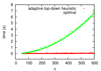
Figure 4: Adaptive Segmentation Timings: Time in seconds versus the number of data points using ECG data. We compare the optimal dynamic programming solution with the top-down heuristic ($k=20$).

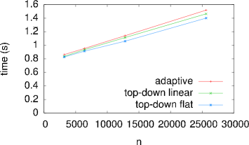
Figure 5: Heuristics timings using random walk data: Time in seconds versus the number of data points ($k=20$).

10 Random Time Series and Segmentation

Intuitively, adaptive algorithms over purely random data are wasteful. To verify this intuition, we generated 10 sequences of Gaussian random noise ($n=200$): each data point takes on a value according to a normal distribution ($\mu=0,\sigma=1$). The average leave-one-out error is presented in Table 3 (top) with model complexity $k=10,20,30$. As expected, the adaptive heuristic shows a slightly worse cross-validation error. However, this is compensated by a slightly better fit error (5%) when compared with the top-down linear heuristic (Fig. 6). On this same figure, we also compare the dynamic programming solution which shows a 10% reduction in fit error for all three models (adaptive, linear, constant/flat), for twice the running time (Fig. 4). The relative errors are not sensitive to the model complexity.

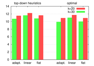
Figure 6: Average Euclidean ($l_{2}$ norm) fit error over synthetic white noise data.

Many chaotic processes such as stock prices are sometimes described as random walk. Unlike white noise, the value of a given data point depends on its neighbors. We generated 10 sequences of Gaussian random walks ($n=200$): starting at the value 0, each data point takes on the value $y_{i}=y_{i-1}+N(0,1)$ where $N(0,1)$ is a value from a normal distribution ($\mu=0,\sigma=1$). The results are presented in Table 3 (bottom) and Fig. 7. The adaptive algorithm improves the leave-one-out error (3%–6%) and the fit error ($\approx 13\%$) over the top-down linear heuristic. Again, the optimal algorithms improve over the heuristics by approximately 10% and the model complexity does not change the relative errors.

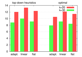
Figure 7: Average Euclidean ($l_{2}$ norm) fit error over synthetic random walk data.

Table 3: Leave-one-out cross-validation error for top-down heuristics on 10 sequences of Gaussian white noise (top) and random walks (bottom) ($n=200$) for various model complexities ($k$)

white noise	adaptive	linear	constant	linear/adaptive
$k=10$	1.07	1.05	1.06	98%
$k=20$	1.21	1.17	1.14	97%
$k=30$	1.20	1.17	1.16	98%

random walks	adaptive	linear	constant	linear/adaptive
$k=10$	1.43	1.51	1.43	106%
$k=20$	1.16	1.21	1.19	104%
$k=30$	1.03	1.06	1.06	103%

11 Stock Market Prices and Segmentation

Creating, searching and identifying stock market patterns is sometimes done using segmentation algorithms [48]. Keogh and Kasetty suggest [28] that stock market data is indistinguishable from random walks. If so, the good results from the previous section should carry over. However, the random walk model has been strongly rejected using variance estimators [36]. Moreover, Sornette [41] claims stock markets are akin to physical systems and can be predicted.

Many financial market experts look for patterns and trends in the historical stock market prices, and this approach is called “technical analysis” or “charting” [4, 6, 15]. If you take into account “structural breaks,” some stock market prices have detectable locally stationary trends [13]. Despite some controversy, technical analysis is a Data Mining topic [44, 20, 26].

We segmented daily stock prices from dozens of companies [1]. Ignoring stock splits, we pick the first 200 trading days of each stock or index. The model complexity varies $k=10,20,30$ so that the number of intervals can range from 5 to 30. We compute the segmentation error using 3 top-down heuristics: adaptive, linear and constant (see Table 4 for some of the result). As expected, the adaptive heuristic is more accurate than the top-down linear heuristic (the gains are between 4% and 11%). The leave-one-out cross-validation error is improved with the adaptive heuristic when the model complexity is small. The relative fit error is not sensitive to the model complexity. We observed similar results using other stocks. These results are consistent with our synthetic random walks results. Using all of the historical data available, we plot the 3 segmentations for Microsoft stock prices (see Fig. 9). The line is the regression polynomial over each interval and only 150 data points out of 5,029 are shown to avoid clutter. Fig. 8 shows the average fit error for all 3 segmentation models: in order to average the results, we first normalized the errors of each stock so that the optimal adaptive is 1.0. These results are consistent with the random walk results (see Fig. 7) and they indicate that the adaptive model is a better choice than the piecewise linear model.

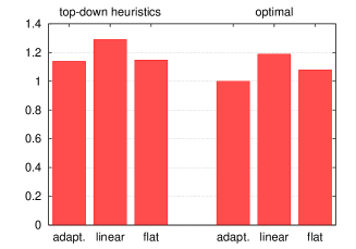
Figure 8: Average Euclidean ($l_{2}$ norm) fit error over 14 different stock prices, for each stock, the error was normalized ($1=$ optimal adaptive segmentation). The complexity is set at 20 ($k=20$) but relative results are not sensitive to the complexity.

Table 4: Euclidean segmentation error ($l_{2}$ norm) and cross-validation error for $k=10,20,30$: lower is better.

		fit error				leave one out error
	adaptative	linear	constant	linear/adaptive	adaptative	linear	constant	linear/adaptive
Google	79.3	87.6	88.1	110%	2.6	2.7	2.8	104%
Sun Microsystems	23.1	26.5	21.7	115%	1.5	1.5	1.4	100%
Microsoft	14.4	15.5	15.5	108%	1.1	1.1	1.1	100%
Adobe	15.3	16.4	14.7	107%	1.1	1.1	1.2	100%
ATI	8.6	9.5	8.1	110%	0.8	0.9	0.8	113%
Autodesk	9.8	10.9	10.4	111%	0.9	0.9	0.9	100%
Conexant	32.6	34.4	32.6	106%	1.7	1.7	1.7	100%
Hyperion	39.0	41.4	38.9	106%	1.9	2.0	1.7	105%
Logitech	6.7	8.0	6.3	119%	0.7	0.8	0.7	114%
NVidia	13.4	15.2	12.4	113%	1.0	1.1	1.0	110%
Palm	51.7	54.2	48.2	105%	1.9	2.0	2.0	105%
RedHat	125.2	147.3	145.3	118%	3.7	3.9	3.7	105%
RSA	17.1	19.3	15.1	113%	1.3	1.3	1.3	100%
Sandisk	13.6	15.6	12.1	115%	1.1	1.1	1.0	100%
Google	52.1	59.1	52.2	113%	2.3	2.4	2.4	104%
Sun Microsystems	13.9	16.5	13.8	119%	1.4	1.4	1.4	100%
Microsoft	10.5	12.3	11.1	117%	1.0	1.1	1.0	110%
Adobe	8.5	9.4	8.3	111%	1.1	1.0	1.1	91%
ATI	5.2	6.1	5.1	117%	0.7	0.7	0.7	100%
Autodesk	6.5	7.2	6.2	111%	0.8	0.8	0.8	100%
Conexant	21.0	22.3	21.8	106%	1.4	1.4	1.5	100%
Hyperion	26.0	29.6	27.7	114%	1.8	1.8	1.7	100%
Logitech	4.2	4.9	4.2	117%	0.7	0.7	0.7	100%
NVidia	9.1	10.7	9.1	118%	0.9	1.0	1.0	111%
Palm	33.8	35.2	31.8	104%	1.9	1.9	1.8	100%
RedHat	77.7	88.2	82.8	114%	3.6	3.6	3.5	100%
RSA	9.8	10.6	10.9	108%	1.2	1.1	1.2	92%
Sandisk	9.0	10.6	8.5	118%	1.0	1.0	0.9	100%
Google	37.3	42.7	39.5	114%	2.2	2.2	2.3	100%
Sun Microsystems	11.7	13.2	11.6	113%	1.4	1.4	1.4	100%
Microsoft	7.5	9.2	8.4	123%	1.0	1.0	1.0	100%
Adobe	6.2	6.8	6.2	110%	1.0	0.9	1.0	90%
ATI	3.6	4.5	3.7	125%	0.7	0.7	0.7	100%
Autodesk	4.7	5.5	4.9	117%	0.8	0.7	0.8	87%
Conexant	16.6	17.6	15.9	106%	1.4	1.4	1.4	100%
Hyperion	18.9	21.5	18.4	114%	1.7	1.7	1.6	100%
Logitech	3.2	3.7	3.1	116%	0.7	0.6	0.7	86%
NVidia	6.9	8.6	6.9	125%	0.9	0.9	0.9	100%
Palm	24.5	25.9	22.5	106%	1.8	1.8	1.8	100%
RedHat	58.1	65.2	58.3	112%	3.8	3.8	3.6	100%
RSA	7.1	8.7	7.3	123%	1.2	1.2	1.2	100%
Sandisk	6.5	7.6	6.4	117%	1.0	1.0	0.9	100%

Figure 9: Microsoft historical daily stock prices (close) segmented by the adaptive top-down (top), linear top-down (middle), and constant top-down (bottom) heuristics. For clarity, only 150 data points out of 5,029 are shown.

12 ECGs and Segmentation

Electrocardiograms (ECGs) are records of the electrical voltage in the heart. They are one of the primary tool in screening and diagnosis of cardiovascular diseases. The resulting time series are nearly periodic with several commonly identifiable extrema per pulse including reference points P, Q, R, S, and T (see Fig. 10). Each one of the extrema has some importance:

• a missing P extrema may indicate arrhythmia (abnormal heart rhythms);

• a large Q value may be a sign of scarring;

• the somewhat flat region between the S and T points is called the ST segment and its level is an indicator of ischemia [34].

ECG segmentation models, including the piecewise linear model [43, 47], are used for compression, monitoring or diagnosis.

Figure 10: A typical ECG pulse with PQRST reference points.

We use ECG samples from the MIT-BIH Arrhythmia Database [22]. The signals are recorded at a sampling rate of 360 samples per second with 11 bits resolution. Prior to segmentation, we choose time intervals spanning 300 samples (nearly 1 second) centered around the QRS complex. We select 5 such intervals by a moving window in the files of 6 different patients (“100.dat”, “101.dat”, “102.dat”, “103.dat”, “104.dat”, “105.dat”). The model complexity varies $k=10,20,30$.

Table 5: Comparison of top-down heuristics on ECG data ($n=200$) for various model complexities: segmentation error and leave-one-out cross-validation error.

Fit error for $k=10,20,30$. patient adaptive linear constant linear/adaptive 100 99.0 110.0 116.2 111% 101 142.2 185.4 148.7 130% 102 87.6 114.7 99.9 131% 103 215.5 300.3 252.0 139% 104 124.8 153.1 170.2 123% 105 178.5 252.1 195.3 141% average 141.3 185.9 163.7 132% 100 46.8 53.1 53.3 113% 101 55.0 65.3 69.6 119% 102 42.2 48.0 50.2 114% 103 88.1 94.4 131.3 107% 104 53.4 53.4 84.1 100% 105 52.4 61.7 97.4 118% average 56.3 62.6 81.0 111% 100 33.5 34.6 34.8 103% 101 32.5 33.6 40.8 103% 102 30.0 32.4 35.3 108% 103 59.8 63.7 66.5 107% 104 29.9 30.3 48.0 101% 105 35.6 37.7 60.2 106% average 36.9 38.7 47.6 105% Leave-one-out error for $k=10,20,30$.

patient	adaptive	linear	constant	linear/adaptive
100	3.2	3.3	3.7	103%
101	3.8	4.5	4.3	118%
102	4.0	4.1	3.5	102%
103	4.6	5.7	5.5	124%
104	4.3	4.1	4.3	95%
105	3.6	4.2	4.5	117%
average	3.9	4.3	4.3	110%
100	2.8	2.8	3.5	100%
101	3.3	3.3	3.6	100%
102	3.3	3.0	3.4	91%
103	2.9	3.1	4.7	107%
104	3.8	3.8	3.6	100%
105	2.4	2.5	3.6	104%
average	3.1	3.1	3.7	100%
100	2.8	2.2	3.3	79%
101	2.9	2.9	3.6	100%
102	3.3	2.9	3.3	88%
103	3.7	3.1	4.4	84%
104	3.2	3.2	3.5	100%
105	2.1	2.1	3.4	100%
average	3.0	2.7	3.6	90%

The segmentation error as well as the leave-one-out error are given in Table 5 for each patient and they are plotted in Fig. 11 in aggregated form, including the optimal errors. With the same model complexity, the adaptive top-down heuristic is better than the linear top-down heuristic (>5%), but more importantly, we reduce the leave-one-out cross-validation error as well for small model complexities. As the model complexity increases, the adaptive model eventually has a slightly worse cross-validation error. Unlike for the random walk and stock market data, the piecewise constant model is no longer competitive in this case. The optimal solution, in this case, is far more competitive with an improvement of approximately $30\%$ of the heuristics, but the relative results are the same.

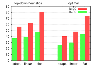
Figure 11: Average Euclidean ($l_{2}$ norm) fit error over ECGs for 6 different patients.

13 Conclusion and Future Work

We argue that if one requires a multimodel segmentation including flat and linear intervals, it is better to segment accordingly instead of post-processing a piecewise linear segmentation. Mixing drastically different interval models (monotonic and linear) and offering richer, more flexible segmentation models remains an important open problem.

To ease comparisons accross different models, we propose a simple complexity model based on counting the number of regressors. As supporting evidence that mixed models are competitive, we consistently improved the accuracy by 5% and 13% respectively without increasing the cross-validation error over white noise and random walk data. Moreover, whether we consider stock market prices of ECG data, for small model complexity, the adaptive top-down heuristic is noticeably better than the commonly used top-down linear heuristic. The adaptive segmentation heuristic is not significantly harder to implement nor slower than the top-down linear heuristic.

We proved that optimal adaptive time series segmentations can be computed in quadratic time, when the model complexity and the polynomial degree are small. However, despite this low complexity, optimal segmentation by dynamic programming is not an option for real-world time series (see Fig. 4). With reason, some researchers go as far as not even discussing dynamic programming as an alternative [27]. In turn, we have shown that adaptive top-down heuristics can be implemented in linear time after the linear time computation of a buffer. In our experiments, for a small model complexity, the top-down heuristics are competitive with the dynamic programming alternative which sometimes offer small gains ($10\%$).

Future work will investigate real-time processing for online applications such as high frequency trading [48] and live patient monitoring. An “amnesic” approach should be tested [39].

14 Acknowledgments

The author wishes to thank Owen Kaser of UNB, Martin Brooks of NRC, and Will Fitzgerald of NASA Ames for their insightful comments.

References

- [1] Yahoo! Finance. last accessed June, 2006.
- [2] S. Abiteboul, R. Agrawal, et al. The Lowell Database Research Self Assessment. Technical report, Microsoft, 2003.
- [3] D. M. Allen. The Relationship between Variable Selection and Data Agumentation and a Method for Prediction. Technometrics, 16(1):125–127, 1974.
- [4] S. Anand, W.-N. Chin, and S.-C. Khoo. Charting patterns on price history. In ICFP’01, pages 134–145, New York, NY, USA, 2001. ACM Press.
- [5] C. G. F. Atkeson, A. W. F. Moore, and S. F. Schaal. Locally Weighted Learning. Artificial Intelligence Review, 11(1):11–73, 1997.
- [6] R. Balvers, Y. Wu, and E. Gilliland. Mean reversion across national stock markets and parametric contrarian investment strategies. Journal of Finance, 55:745–772, 2000.
- [7] R. Bellman and R. Roth. Curve fitting by segmented straight lines. J. Am. Stat. Assoc., 64:1079–1084, 1969.
- [8] M. Birattari, G. Bontempi, and H. Bersini. Lazy learning for modeling and control design. Int. J. of Control, 72:643–658, 1999.
- [9] H. J. Breaux. A modification of Efroymson’s technique for stepwise regression analysis. Commun. ACM, 11(8):556–558, 1968.
- [10] M. Brooks, Y. Yan, and D. Lemire. Scale-based monotonicity analysis in qualitative modelling with flat segments. In IJCAI’05, 2005.
- [11] K. P. Burnham and D. R. Anderson. Multimodel inference: understanding aic and bic in model selection. In Amsterdam Workshop on Model Selection, 2004.
- [12] S. Chardon, B. Vozel, and K. Chehdi. Parametric blur estimation using the generalized cross-validation. Multidimensional Syst. Signal Process., 10(4):395–414, 1999.
- [13] K. Chaudhuri and Y. Wu. Random walk versus breaking trend in stock prices: Evidence from emerging markets. Journal of Banking & Finance, 27:575–592, 2003.
- [14] D. L. Donoho and I. M. Johnstone. Ideal spatial adaptation by wavelet shrinkage. Biometrika, 81:425–455, 1994.
- [15] E. F. Fama and K. R. French. Permanent and temporary components of stock prices. Journal of Political Economy, 96:246–273, 1988.
- [16] W. Fitzgerald, D. Lemire, and M. Brooks. Quasi-monotonic segmentation of state variable behavior for reactive control. In AAAI’05, 2005.
- [17] D. P. Foster and E. I. George. The risk inflation criterion for multiple regression. Annals of Statistics, 22:1947–1975, 1994.
- [18] H. Friedl and E. Stampfer. Encyclopedia of Environmetrics, chapter Cross-Validation. Wiley, 2002.
- [19] J. Friedman. Multivariate adaptive regression splines. Annals of Statistics, 19:1–141, 1991.
- [20] T. Fu, F. Chung, R. Luk, and C. Ng. Financial Time Series Indexing Based on Low Resolution Clustering. ICDM-2004 Workshop on Temporal Data Mining, 2004.
- [21] D. G. Galati and M. A. Simaan. Automatic decomposition of time series into step, ramp, and impulse primitives. Pattern Recognition, 39(11):2166–2174, November 2006.
- [22] A. L. Goldberger, L. A. N. Amaral, et al. PhysioBank, PhysioToolkit, and PhysioNet. Circulation, 101(23):215–220, 2000.
- [23] N. Haiminen and A. Gionis. Unimodal segmentation of sequences. In ICDM’04, 2004.
- [24] J. Han, W. Gong, and Y. Yin. Mining segment-wise periodic patterns in time-related databases. In KDD’98, 1998.
- [25] T. Hastie, R. Tibshirani, and J. Friedman. Elements of Statistical Learning: Data Mining, Inference and Prediction. Springer-Verlag, 2001.
- [26] J. Kamruzzaman, RA Sarker, and I. Ahmad. SVM based models for predicting foreign currency exchange rates. ICDM 2003, pages 557–560, 2003.
- [27] E. J. Keogh, S. Chu, D. Hart, and M. J. Pazzani. An online algorithm for segmenting time series. In ICDM’01, pages 289–296, Washington, DC, USA, 2001. IEEE Computer Society.
- [28] E. J. Keogh and S. F. Kasetty. On the Need for Time Series Data Mining Benchmarks: A Survey and Empirical Demonstration. Data Mining and Knowledge Discovery, 7(4):349–371, 2003.
- [29] E. J. Keogh and M. J. Pazzani. An enhanced representation of time series which allows fast and accurate classification, clustering and relevance feedback. In KDD’98, pages 239–243, 1998.
- [30] J. Kleinberg and É. Tardos. Algorithm design. Pearson/Addison-Wesley, 2006.
- [31] D. Lemire. Wavelet-based relative prefix sum methods for range sum queries in data cubes. In CASCON 2002. IBM, October 2002.
- [32] D. Lemire, M. Brooks, and Y. Yan. An optimal linear time algorithm for quasi-monotonic segmentation. In ICDM’05, 2005.
- [33] D. Lemire and O. Kaser. Hierarchical bin buffering: Online local moments for dynamic external memory arrays. submitted in February 2004.
- [34] D. Lemire, C. Pharand, et al. Wavelet time entropy, t wave morphology and myocardial ischemia. IEEE Transactions in Biomedical Engineering, 47(7), July 2000.
- [35] M. Lindstrom. Penalized estimation of free-knot splines. Journal of Computational and Graphical Statistics, 1999.
- [36] A. W. Lo and A. C. MacKinlay. Stock Market Prices Do Not Follow Random Walks: Evidence from a Simple Specification Test. The Review of Financial Studies, 1(1):41–66, 1988.
- [37] Z. Luo and G. Wahba. Hybrid adaptive splines. Journal of the American Statistical Association, 1997.
- [38] G. Monari and G. Dreyfus. Local Overfitting Control via Leverages. Neural Comp., 14(6):1481–1506, 2002.
- [39] T. Palpanas, T. Vlachos, E. Keogh, D. Gunopulos, and W. Truppel. Online amnesic approximation of streaming time series. In ICDE 2004, 2004.
- [40] E. Pednault. Minimum length encoding and inductive inference. In G. Piatetsky-Shapiro and W. Frawley, editors, Knowledge Discovery in Databases. AAAI Press, 1991.
- [41] D. Sornette. Why Stock Markets Crash: Critical Events in Complex Financial Systems. Princeton University Press, 2002.
- [42] E. Terzi and P. Tsaparas. Efficient algorithms for sequence segmentation. In SDM’06, 2006.
- [43] I. Tomek. Two algorithms for piecewise linear continuous approximations of functions of one variable. IEEE Trans. on Computers, C-23:445–448, April 1974.
- [44] P. Tse and J. Liu. Mining Associated Implication Networks: Computational Intermarket Analysis. ICDM 2002, pages 689–692, 2002.
- [45] K.i Tsuda, G. Rätsch, S. Mika, and K.-R. Müller. Learning to predict the leave-one-out error. In NIPS*2000 Workshop: Cross-Validation, Bootstrap and Model Selection, 2000.
- [46] K. T. Vasko and H. T. T. Toivonen. Estimating the number of segments in time series data using permutation tests. In ICDM’02, 2002.
- [47] H. J. L. M. Vullings, M. H. G. Verhaegen, and H. B. Verbruggen. ECG segmentation using time-warping. In IDA’97, pages 275–285, London, UK, 1997. Springer-Verlag.
- [48] H. Wu, B. Salzberg, and D. Zhang. Online event-driven subsequence matching over financial data streams. In SIGMOD’04, pages 23–34, New York, NY, USA, 2004. ACM Press.
- [49] Y. Zhu and D. Shasha. Query by humming: a time series database approach. Proc. of SIGMOD, 2003.