Optimal and Suboptimal Finger Selection Algorithms for MMSE Rake Receivers in Impulse Radio Ultra-Wideband Systems${}^{\textrm{\small{0}}}$

Abstract

The problem of choosing the optimal multipath components to be employed at a minimum mean square error (MMSE) selective Rake receiver is considered for an impulse radio ultra-wideband system. First, the optimal finger selection problem is formulated as an integer programming problem with a non-convex objective function. Then, the objective function is approximated by a convex function and the integer programming problem is solved by means of constraint relaxation techniques. The proposed algorithms are suboptimal due to the approximate objective function and the constraint relaxation steps. However, they perform better than the conventional finger selection algorithm, which is suboptimal since it ignores the correlation between multipath components, and they can get quite close to the optimal scheme that cannot be implemented in practice due to its complexity. In addition to the convex relaxation techniques, a genetic algorithm (GA) based approach is proposed, which does not need any approximations or integer relaxations. This iterative algorithm is based on the direct evaluation of the objective function, and can achieve near-optimal performance with a reasonable number of iterations. Simulation results are presented to compare the performance of the proposed finger selection algorithms with that of the conventional and the optimal schemes.

Index Terms— Ultra-wideband (UWB), impulse radio (IR), MMSE Rake receiver, convex optimization, integer programming, genetic algorithm (GA).

I Introduction

Since the US Federal Communications Commission (FCC) approved the limited use of ultra-wideband (UWB) technology [1], communications systems that employ UWB signals have drawn considerable attention. A UWB signal is defined to be one that possesses an absolute bandwidth larger than $500$MHz or a relative bandwidth larger than 20% and can coexist with incumbent systems in the same frequency range due to its large spreading factor and low power spectral density. UWB technology holds great promise for a variety of applications such as short-range high-speed data transmission and precise location estimation.

Commonly, impulse radio (IR) systems, which transmit very short pulses with a low duty cycle, are employed to implement UWB systems ([2]-[6]). In an IR system, a train of pulses is sent and information is usually conveyed by the positions or the amplitudes of the pulses, which correspond to pulse position modulation (PPM) and pulse amplitude modulation (PAM), respectively. In order to prevent catastrophic collisions among different users and thus provide robustness against multiple-access interference, each information symbol is represented by a sequence of pulses, and the positions of the pulses within that sequence are determined by a pseudo-random time-hopping (TH) sequence specific to each user [2]. The number $N_{f}$ of pulses representing one information symbol can also be interpreted as pulse combining gain.

Typically, users in an IR-UWB system employ Rake receivers to collect energy from different multipath components. A Rake receiver combining all the paths of the incoming signal is called an all-Rake (ARake) receiver. Since a UWB signal has a very wide bandwidth, the number of resolvable multipath components is usually very large. Hence, an ARake receiver is not implemented in practice due to its complexity. However, it serves as a benchmark for the performance of more practical Rake receivers. A feasible implementation of multipath diversity combining can be obtained by a selective-Rake (SRake) receiver, which combines the $M$ best, out of $L$, multipath components [7]. Those $M$ best components are determined by a finger selection algorithm. For a maximal ratio combining (MRC) Rake receiver, the paths with highest signal-to-noise ratios (SNRs) are selected, which is an optimal scheme in the absence of interfering users and inter-symbol interference (ISI) [8]-[10]. For a minimum mean square error (MMSE) Rake receiver, the “conventional” finger selection algorithm can be defined as choosing the paths with highest signal-to-interference-plus-noise ratios (SINRs). This conventional scheme is not necessarily optimal since it ignores the correlation of the noise terms at different multipath components. The finger selection problem is also studied in the context of CDMA downlink equalization, and recursive sequential search (RSS) and heuristic arguments of interference cancellation are proposed to determine finger locations [11]. The RSS algorithm selects the fingers one by one in a sequential manner, which reduces the computationally complexity significantly; however, it may be quite suboptimal depending on the correlation structure of the noise components. The heuristic arguments are employed to determine finger locations when the number of fingers is larger than the number of multipath components, which is not applicable in our case due to a large number of multipath components in a typical UWB channel. In [12], asymptotic optimality of “regular” finger assignments is investigated. However, the behavior of the algorithms for a small number of fingers, and performance of other schemes without “regular” assignments are not specified. Finally, the finger selection problem is considered in [13] for UWB systems, and a matching pursuit-based technique with a quadratic constraint is proposed. However, the performance of the algorithm depends heavily on a parameter of the quadratic constraint, which needs to be determined empirically.

In this paper, unlike the previous approaches, we provide a complete optimization theoretical framework for the finger selection problem for MMSE SRake receivers. First, we formulate the optimal MMSE SRake as a nonconvex, integer-constrained optimization, in which the aim is to choose the finger locations of the receiver so as to maximize the overall SINR. While computing the optimal finger selection is NP-hard, we present several relaxation methods to turn the (approximate) problem into convex optimization problems that can be very efficiently solved by interior-point methods, which are polynomial-time in the worst case, and are very fast in practice. These optimal finger selection relaxations produce significantly higher average SINR than the conventional one that ignores the correlations, and represent a numerically efficient way to strike a balance between SINR optimality and computational tractability. Moreover, we propose a genetic algorithm (GA) based scheme, which performs finger selection by iteratively evaluating the overall SINR expression. Using this technique, near-optimal solutions can be obtained in many cases with a degree of complexity that is much lower than that of optimal search.

The remainder of this paper is organized as follows. Section II describes the transmitted and received signal models in a multiuser frequency-selective environment. The finger selection problem is formulated and the optimal algorithm is described in Section III, followed by a brief description of the conventional algorithm in Section IV. In Section V, two convex relaxations of the optimal finger selection algorithm, based on an approximate SINR expression and integer constraint relaxation techniques, are proposed. The GA-based approach is presented in Section VI as an alternative to the suboptimal schemes based on convex relaxations. Simulation results are presented in Section VII, and concluding remarks are made in the last section.

II Signal Model

We consider a synchronous, binary phase shift keyed TH-IR system with $K$ users, in which the transmitted signal from user $k$ is represented by:

$$s^{(k)}_{{\rm{tx}}}(t)=\sqrt{\frac{E_{k}}{N_{f}}}\sum_{j=-\infty}^{\infty}d^{(k)}_{j}\,b^{(k)}_{\lfloor j/N_{f}\rfloor}p_{{\rm{tx}}}(t-jT_{f}-c^{(k)}_{j}T_{c}),$$ (1)

where $p_{{\rm{tx}}}(t)$ is the transmitted UWB pulse, $E_{k}$ is the bit energy of user $k$, $T_{f}$ is the “frame” time, $N_{f}$ is the number of pulses representing one information symbol, and $b^{(k)}_{\lfloor j/N_{f}\rfloor}\in\{+1,-1\}$ is the binary information symbol transmitted by user $k$. In order to allow the channel to be shared by many users and avoid catastrophic collisions, a TH sequence $\{c^{(k)}_{j}\}$, where $c^{(k)}_{j}\in\{0,1,...,N_{c}-1\}$, is assigned to each user. This TH sequence provides an additional time shift of $c^{(k)}_{j}T_{c}$ seconds to the $j$th pulse of the $k$th user where $T_{c}$ is the chip interval and is chosen to satisfy $T_{c}\leq T_{f}/N_{c}$ in order to prevent the pulses from overlapping. We assume $T_{f}=N_{c}T_{c}$ without loss of generality. The random polarity codes $d^{(k)}_{j}$ are binary random variables taking values $\pm 1$ with equal probability [14]-[16].

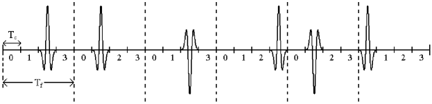
Figure 1: An example time-hopping impulse radio signal with pulse-based polarity randomization, where $N_{f}=6$, $N_{c}=4$, the time hopping sequence is {2,1,2,3,1,0} and the polarity codes are {+1,+1,-1,+1,-1,+1}.

An example TH-IR signal is shown in Figure 1, where six pulses are transmitted for each information symbol ($N_{f}=6$) with the TH sequence $\{2,1,2,3,1,0\}$.

Consider the discrete presentation of the channel, $\boldsymbol{\alpha}^{(k)}=[\alpha_{1}^{(k)}\cdots\alpha_{L}^{(k)}]$ for user $k$, where $L$ is assumed to be the number of multipath components for each user, and $T_{c}$ is the multipath resolution. Note that this channel model is quite general in that it can model any channel of the form $\sum_{l=1}^{\hat{L}}\hat{\alpha}_{l}^{(k)}\delta(t-\hat{\tau}_{l}^{(k)})$ if the channel is bandlimited to $1/T_{c}$ [17]. Then, the received signal can be expressed as

$$r(t)=\sum_{k=1}^{K}\sqrt{\frac{E_{k}}{N_{f}}}\sum_{j=-\infty}^{\infty}\sum_{l=1}^{L}\alpha_{l}^{(k)}d^{(k)}_{j}\,b^{(k)}_{\lfloor j/N_{f}\rfloor}p_{{\rm{rx}}}(t-jT_{f}-c^{(k)}_{j}T_{c}-(l-1)T_{c})+\sigma_{n}n(t),$$ (2)

where $p_{{\rm{rx}}}(t)$ is the received unit-energy UWB pulse, which is usually modelled as the derivative of $p_{{\rm{tx}}}(t)$ due to the effects of the receive antenna, and $n(t)$ is zero mean white Gaussian noise with unit spectral density.

We assume that the TH sequence is constrained to the set $\{0,1,\ldots,N_{T}-1\}$, where $N_{T}\leq N_{c}-L$, so that there is no inter-frame interference (IFI). However, the proposed algorithms are valid for scenarios with IFI as well, and this assumption is made merely to simplify the expressions throughout the paper. From the analysis in [18], the results of this paper can easily be extended to the IFI case as well.

Due to the high resolution of UWB signals, chip-rate and frame-rate sampling are not very practical for such systems. In order to have a lower sampling rate, the received signal can be correlated with symbol-length template signals that enable symbol-rate sampling of the correlator output [19]. The template signal for the $l$th path of the incoming signal can be expressed as

$$s_{{\rm{temp}},l}^{(1)}(t)=\sum_{j=iN_{f}}^{(i+1)N_{f}-1}d^{(1)}_{j}\,p_{{\rm{rx}}}(t-jT_{f}-c^{(1)}_{j}T_{c}-(l-1)T_{c}),$$ (3)

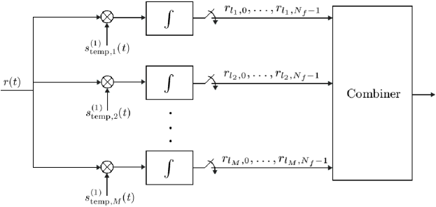
Figure 2: The receiver structure. There are $M$ multipath components, which are combined by the MMSE combiner.

for the $i$th information symbol, where we consider user $1$ as the desired user, without loss of generality. In other words, by using a correlator for each multipath component that we want to combine, we can have symbol-rate sampling at each branch, as shown in Figure 2.

Note that the use of such template signals results in equal gain combining (EGC) of different frame components. This may not be optimal under some conditions (see [18] for (sub)optimal schemes). However, it is very practical since it facilitates symbol-rate sampling. Since we consider a system that employs template signals of the form (3), i.e. EGC of frame components, it is sufficient to consider the problem of selection of the optimal paths for just one frame. Hence, we assume $N_{f}=1$ without loss of generality.

Let ${\mathcal{L}}=\{l_{1},\ldots,l_{M}\}$ denote the set of multipath components that the receiver collects (Figure 2). At each branch, the signal is effectively passed through a matched filter (MF) matched to the related template signal in (3) and sampled once for each symbol. Then, the discrete signal for the $l$th path can be expressed, for the $i$th information symbol, as²

$$r_{l}={\bf s}^{T}_{l}{\bf A}{\bf b}_{i}+n_{l},$$ (4)

for $l=l_{1},\ldots,l_{M}$, where ${\bf A}=\textrm{diag}\{\sqrt{E_{1}},\ldots,\sqrt{E_{K}}\}$, ${\bf b}_{i}=[b_{i}^{(1)}\cdots b_{i}^{(K)}]^{T}$ and $n_{l}\sim\mathcal{N}(0\,,\,\sigma_{n}^{2})$. ${\bf s}_{l}$ is a $K\times 1$ vector, which can be expressed as a sum of the desired signal part (SP) and multiple-access interference (MAI) terms:

$${\bf s}_{l}={\bf s}_{l}^{({\rm{SP}})}+{\bf s}_{l}^{({\rm{MAI}})},$$ (5)

where the $k$th elements can be expressed as

$$\left[{\bf s}_{l}^{({\rm{SP}})}\right]_{k} =\begin{cases}\alpha_{l}^{(1)},\quad\quad k=1\\ 0,\quad\quad\quad\,k=2,\ldots,K\end{cases}\textrm{and}$$ (6)

$$\left[{\bf s}_{l}^{({\rm{MAI}})}\right]_{k} =\begin{cases}0,\quad\quad\quad\quad\quad\quad\quad\quad\quad\quad\,\,\,k=1\\ d_{1}^{(1)}d_{1}^{(k)}\sum_{m=1}^{L}\alpha_{m}^{(k)}I_{l,m}^{(k)},\quad\quad k=2,\ldots,K\end{cases},$$ (7)

with $I_{l,m}^{(k)}$ being the indicator function that is equal to $1$ if the $m$th path of user $k$ collides with the $l$th path of user $1$, and $0$ otherwise.

III Problem Formulation and Optimal Solution

The problem is to choose the optimal set of multipath components, $\mathcal{L}=\{l_{1},\ldots,l_{M}\}$, that maximizes the overall SINR of the system. In other words, we need to choose the best samples from the $L$ received samples $r_{l}$, $l=1,\ldots,L$, as shown in (4).

To reformulate this combinatorial problem, we first define an $M\times L$ selection matrix ${\bf X}$ as follows: $M$ of the columns of ${\bf X}$ are the unit vectors ${\bf e}_{1},\ldots,{\bf e}_{M}$ (${\bf e}_{i}$ having a $1$ at its $i$th position and zero elements for all other entries), and the other columns are all zero vectors. The column indices of the unit vectors determine the subset of the multipath components that are selected. For example, for $L=4$ and $M=2$, ${\bf X}=\begin{bmatrix}0\,\,1\,\,0\,\,0\\ 0\,\,0\,\,1\,\,0\end{bmatrix}$ chooses the second and third multipath components.

Using the selection matrix ${\bf X}$, we can express the vector of received samples from $M$ multipath components as

$${\bf r}={\bf X}{\bf S}{\bf A}{\bf b}_{i}+{\bf X}{\bf n},$$ (8)

where ${\bf n}$ is the vector of thermal noise components ${\bf n}=[n_{1}\cdots n_{L}]^{T}$, and ${\bf S}$ is the signature matrix given by ${\bf S}=[{\bf s}_{1}\cdots{\bf s}_{L}]^{T}$, with ${\bf s}_{l}$ as in (5).

From (5)-(7), (8) can be expressed as

$${\bf r}=b_{i}^{(1)}\sqrt{E_{1}}{\bf X}\boldsymbol{\alpha}^{(1)}+{\bf X}{\bf S}^{({\rm{MAI}})}{\bf A}{\bf b}_{i}+{\bf X}{\bf n},$$ (9)

where ${\bf S}^{({\rm{MAI}})}$ is the MAI part of the signature matrix ${\bf S}$.

Then, the linear MMSE receiver can be expressed as

$$\hat{b}_{i}=\textrm{sign}\{\boldsymbol{\theta}^{T}{\bf r}\},$$ (10)

where the MMSE weight vector is given by [20]

$$\boldsymbol{\theta}={\bf R}^{-1}{\bf X}\boldsymbol{\alpha}^{(1)},$$ (11)

with ${\bf R}$ being the correlation matrix of the noise term:

$${\bf R}={\bf X}{\bf S}^{({\rm{MAI}})}{\bf A}^{2}({\bf S}^{({\rm{MAI}})})^{T}{\bf X}^{T}+\sigma_{n}^{2}{\bf I}.$$ (12)

The overall SINR of the system can be expressed as

$${\rm{SINR}}({\bf X})=\frac{E_{1}}{\sigma_{n}^{2}}(\boldsymbol{\alpha}^{(1)})^{T}{\bf X}^{T}\left({\bf I}+\frac{1}{\sigma_{n}^{2}}{\bf X}{\bf S}^{({\rm{MAI}})}{\bf A}^{2}({\bf S}^{({\rm{MAI}})})^{T}{\bf X}^{T}\right)^{-1}{\bf X}\boldsymbol{\alpha}^{(1)}.$$ (13)

Hence, the optimal finger selection problem can be formulated as finding ${\bf X}$ that solves the following problem:

$$\textrm{maximize}\,\,{\rm{SINR}}({\bf X}),$$ (14)

subject to the constraint that ${\bf X}$ has the previously defined structure. Note that the objective function to be maximized is not concave and the optimization variable ${\bf X}$ takes binary values, with the previously defined structure. In other words, two major difficulties arise in solving (14) globally: nonconvex optimization and integer constraints. Either makes the problem NP-hard. Therefore, it is an intractable optimization problem in this general form.

IV Conventional Algorithm

Instead of the solving the problem in (14), the “conventional” finger selection algorithm chooses the $M$ paths with largest individual SINRs, where the SINR for the $l$th path can be expressed as

$${\rm{SINR}}_{l}=\frac{E_{1}(\alpha_{l}^{(1)})^{2}}{({\bf s}_{l}^{({\rm{MAI}})})^{T}{\bf A}^{2}{\bf s}_{l}^{({\rm{MAI}})}+\sigma_{n}^{2}},$$ (15)

for $l=1,\ldots,L$.

This algorithm is not optimal because it ignores the correlation of the noise components of different paths. Therefore, it does not always maximize the overall SINR of the system given in (13). For example, the contribution of two highly correlated strong paths to the overall SINR might be worse than the contribution of one strong and one relatively weaker, but uncorrelated, paths. The correlation between the multipath components is the result of the MAI from the interfering users in the system.

V Relaxations of Optimal Finger Selection

Since the optimal solution in (14) is quite difficult, we first consider an approximation of the objective function in (13). When the eigenvalues of $\frac{1}{\sigma_{n}^{2}}{\bf X}{\bf S}^{({\rm{MAI}})}{\bf A}^{2}({\bf S}^{({\rm{MAI}})})^{T}{\bf X}^{T}$ are considerably smaller than $1$, which occurs when the MAI is not very strong compared to the thermal noise, we can approximate the SINR expression in (13) as follows³:

$${\rm{SINR}}({\bf X})\approx\frac{E_{1}}{\sigma_{n}^{2}}(\boldsymbol{\alpha}^{(1)})^{T}{\bf X}^{T}\left({\bf I}-\frac{1}{\sigma_{n}^{2}}{\bf X}{\bf S}^{({\rm{MAI}})}{\bf A}^{2}({\bf S}^{({\rm{MAI}})})^{T}{\bf X}^{T}\right){\bf X}\boldsymbol{\alpha}^{(1)},$$ (16)

which can be expressed as

$${\rm{SINR}}({\bf X})\approx\frac{E_{1}}{\sigma_{n}^{2}}\{\,(\boldsymbol{\alpha}^{(1)})^{T}{\bf X}^{T}{\bf X}\boldsymbol{\alpha}^{(1)}-\frac{1}{\sigma_{n}^{2}}\boldsymbol{\alpha}^{(1)}{\bf X}^{T}{\bf X}{\bf S}^{({\rm{MAI}})}{\bf A}^{2}({\bf S}^{({\rm{MAI}})})^{T}{\bf X}^{T}{\bf X}\boldsymbol{\alpha}^{(1)}\,\}.$$ (17)

Note that the approximate SINR expression depends on ${\bf X}$ only through ${\bf X}^{T}{\bf X}$. Defining ${\bf x}=[x_{1}\cdots x_{L}]^{T}$ as the diagonal elements of ${\bf X}^{T}{\bf X}$, ${\bf x}=\textrm{diag}\{{\bf X}^{T}{\bf X}\}$, we have $x_{i}=1$ if the $i$th path is selected, and $x_{i}=0$ otherwise; and $\sum_{i=1}^{L}x_{i}=M$. Then, we obtain, after some manipulation,

$${\rm{SINR}}({\bf x})=\frac{E_{1}}{\sigma_{n}^{2}}\left\{{\bf q}^{T}{\bf x}-\frac{1}{\sigma_{n}^{2}}{\bf x}^{T}{\bf P}{\bf x}\right\},$$ (18)

where ${\bf q}=[(\alpha_{1}^{(1)})^{2}\cdots(\alpha_{L}^{(1)})^{2}]^{T}$ and ${\bf P}=\textrm{diag}\{\alpha_{1}^{(1)}\cdots\alpha_{L}^{(1)}\}{\bf S}^{({\rm{MAI}})}{\bf A}^{2}({\bf S}^{({\rm{MAI}})})^{T}\textrm{diag}\{\alpha_{1}^{(1)}\cdots\alpha_{L}^{(1)}\}$.

Then, we can formulate the finger selection problem as follows:

minimize $$\frac{1}{\sigma_{n}^{2}}{\bf x}^{T}{\bf P}{\bf x}-{\bf x}^{T}{\bf q}$$

subject to $${\bf x}^{T}{\bf 1}=M,$$

$$x_{i}\in\{0,1\},\quad i=1,\ldots,L.$$ (19)

Note that the objective function is convex since ${\bf P}$ is positive definite, and that the first constraint is linear. However, the integer constraint increases the complexity of the problem. The common way to approximate the solution of an integer constraint problem is to use constraint relaxation. Then, the optimizer will be a continuous value instead of being binary and the problem (V) will be convex. Over the past decade, both powerful theory and efficient numerical algorithms have been developed for nonlinear convex optimization. It is now recognized that the watershed between “easy” and “difficult” optimization problems is not linearity but convexity. For example, the interior-point algorithms for nonlinear convex optimization are very fast, both in theory and in practice: they are provably polynomial time in theory, and in practice usually take about $25$-$40$ times the computational load of solving a least-squares problem of the same dimension to reach a global optimum of a constrained convex optimization problem [21], [22]. The interior-point methods solve convex optimization problems with inequality constraints by applying Newton’s method to a sequence of equality constrained problems, where the Newton’s method is a kind of descent algorithm with the descent direction given by the Newton step [21].

We consider two different relaxation techniques in the following subsections.

V-A Case-1: Relaxation to Sphere

Consider the relaxation of the integer constraint in (V) to a sphere that passes through all possible integer values. Then, the relaxed problem becomes

minimize $$\frac{1}{\sigma_{n}^{2}}{\bf x}^{T}{\bf P}{\bf x}-{\bf x}^{T}{\bf q}$$

subject to $$\,{\bf x}^{T}{\bf 1}=M,$$

$$(2{\bf x}-{\bf 1})^{T}(2{\bf x}-{\bf 1})\leq L.$$ (20)

Note that the problem becomes a convex quadratically constrained quadratic programming (QCQP) problem [21]. Hence it can be solved for global optimality using interior-point algorithms in polynomial time.

V-B Case-2: Relaxation to Hypercube

As an alternative approach, we can relax the integer constraint in (V) to a hypercube constraint and obtain

minimize $$\frac{1}{\sigma_{n}^{2}}{\bf x}^{T}{\bf P}{\bf x}-{\bf x}^{T}{\bf q}$$

subject to $$\,{\bf x}^{T}{\bf 1}=M,$$

$$\,{\bf x}\in[0,1]^{L},$$ (21)

where the hypercube constraint can be expressed as ${\bf x}\succeq\mathbb{0}$ and ${\bf x}\preceq{\bf 1}$, with ${\bf y}\succeq{\bf z}$ meaning that $y_{1}\geq z_{1},\ldots,y_{L}\geq z_{L}$. Note that the problem is now a linearly constrained quadratic programming (LCQP) problem, and can be solved by interior-point algorithms [21] for the optimizer ${\bf x}^{*}$.

V-C Dual Methods

We can also consider the dual problems. For the relaxation to the sphere considered in Section V-A, the Lagrangian for (V-A) can be obtained as

$$\mathcal{L}({\bf x},\lambda,\nu)={\bf x}^{T}\left(\frac{1}{\sigma_{n}^{2}}{\bf P}+\nu{\bf I}\right){\bf x}-{\bf x}^{T}({\bf q}-\lambda{\bf 1}+\nu{\bf 1})-M\lambda,$$ (22)

where $\lambda\in\mathcal{R}$ and $\nu\in\mathcal{R}^{+}$.

After some manipulation, the Lagrange dual function, which is the Lagrangian maximized over the primal variable ${\bf x}$, can be expressed as

$$g(\lambda,\nu)=-\frac{1}{4}\,[{\bf q}+(\nu-\lambda){\bf 1}]^{T}\left(\frac{1}{\sigma_{n}^{2}}{\bf P}+\nu{\bf I}\right)^{-1}[{\bf q}+(\nu-\lambda){\bf 1}]-M\lambda,$$ (23)

Then, the dual problem becomes

$$\textrm{minimize}\quad\frac{1}{4}[{\bf q}+(\nu-\lambda){\bf 1}]^{T}\left(\frac{1}{\sigma_{n}^{2}}{\bf P}+\nu{\bf I}\right)^{-1}[{\bf q}+(\nu-\lambda){\bf 1}]+M\lambda$$ (24)

$$\textrm{subject to}\quad\nu\geq 0,$$ (25)

which can be solved for optimal $\lambda$ and $\nu$ by interior point methods. Or, more simply, the unconstrained problem (24) can be solved using a gradient descent algorithm, and then the optimizer $\bar{\nu}$ is mapped to $\nu^{*}=\max\{0,\bar{\nu}\}$.

After solving for optimal $\lambda$ and $\mu$, the optimizer ${\bf x}^{*}$ is obtained as

$${\bf x}^{*}=\frac{1}{2}\left(\frac{1}{\sigma_{n}^{2}}{\bf P}+\nu^{*}{\bf I}\right)^{-1}[{\bf q}+(\nu^{*}-\lambda^{*}){\bf 1}].$$ (26)

Note that the dual problem (24) has two variables, $\lambda$ and $\nu$, to optimize, compared to $L$ variables, the components of ${\bf x}$, in the primal problem (V-A). However, an $L\times L$ matrix must be inverted for each iteration of the optimization of (24). Therefore, the primal problem may be preferred over the dual problem in certain cases.

Similarly, the dual problem for the relaxation in Section V-B can be obtained from (V-B) as

$$\textrm{minimize}\quad\frac{\sigma_{n}^{2}}{4}({\bf q}+\boldsymbol{\mu}-\boldsymbol{\nu}-\lambda{\bf 1})^{T}{\bf P}^{-1}({\bf q}+\boldsymbol{\mu}-\boldsymbol{\nu}-\lambda{\bf 1})+M\lambda+\boldsymbol{\nu}^{T}{\bf 1}$$ (27)

$$\textrm{subject to}\quad\boldsymbol{\mu},\boldsymbol{\nu}\succeq{\bf 0}.$$ (28)

It is observed from (27) that there are $2L+1$ variables and also $L\times L$ matrix inversion operations for the solution of the dual problem. Therefore, the simpler primal problem (V-B) is considered in the simulations.

V-D Selection of Finger Locations

After solving the approximate problem (V) by means of integer relaxation techniques mentioned above, the finger location estimates are obtained by the indices of the $M$ largest elements of the optimizer ${\bf x}^{*}$.

Both the approximation of the SINR expression by (16) and the integer relaxation steps result in the suboptimality of the solution. Therefore, it may not be very close to the optimal solution in some cases. However, it is expected to perform better than the conventional algorithm most of the time, since it considers the correlation between the multipath components. However, it is not guaranteed that the algorithms based on the convex relaxations of optimal finger selection always beat the conventional one. Since the conventional algorithm is very easy to implement, we can consider a hybrid algorithm in which the final estimate of the convex relaxation algorithm is compared with that of the conventional one, and the one that minimizes the exact SINR expression in (13) is chosen as the final estimate. In this way, the resulting hybrid suboptimal algorithm can get closer to the optimal solution.

VI Finger Selection Using Genetic Algorithms

The algorithms in the previous section convert the optimal finger selection problem into a convex problem by approximating the SINR expression in (13) by a concave function in (18), and by employing the relaxation techniques on the integer constraints. As another way to solve the finger selection problem, we propose a GA based approach, which directly uses the exact SINR expression in (13), and does not employ any relaxation techniques.

VI-A Genetic Algorithm

The GA is an iterative technique for searching for the global optimum of a cost function [23]. The name comes from the fact that the algorithm models the natural selection and survival of the fittest [24].

The GA starts with a population of chromosomes, where each chromosome is represented by a binary string⁵. Let $N_{{\rm{ipop}}}$ denote the number of chromosomes in this population. Then, the fittest $N_{{\rm{pop}}}$ of these chromosomes are selected, according to a fitness function. After that, the fittest $N_{{\rm{good}}}$ chromosomes, which are also called the “parents”, are selected and paired among themselves (pairing step). From each chromosome pair, two new chromosomes are generated, which is called the mating step. In other words, the new population consists of $N_{{\rm{good}}}$ parent chromosomes and $N_{{\rm{good}}}$ children generated from the parents by mating. After the mating step, the mutation stage follows, where some chromosomes (the fittest one in the population can be excluded) are chosen randomly and are slightly modified; that is, some bits in the selected binary string are flipped. After that, the pairing, mating and mutation steps are repeated until a threshold criterion is met.

The GA has been applied to a variety of problems in different areas [23]-[25]. Also, it has recently been employed in the multiuser detection problem [26]-[28]. The main characteristics of the GA algorithm is that it can get close to the optimal solution with low complexity, if the steps of the algorithm are designed appropriately.

VI-B Finger Selection via the GA

In order to be able to employ the GA for the finger selection problem we need to consider how to represent the chromosomes, and how to implement the steps of the iterative optimization scheme.

A natural way to represent a chromosome is to consider the “assignment vector” ${\bf x}$ in (18), which denotes the assignments of the multipath components to the $M$ fingers of the RAKE receiver. In other words, $x_{i}=1$ if the $i$th path is selected, and $x_{i}=0$ otherwise; and $\sum_{i=1}^{L}x_{i}=M$.

Also, the fitness function that should be maximized can be the SINR expression given by (13). Note that, given a value of ${\bf x}$, ${\rm{SINR}}({\bf X})$ can be uniquely evaluated. By choosing this fitness function, the fittest chromosomes of the population correspond to the assignment vectors with the largest SINR values.

Now the pairing, mating and mutation steps need to be designed for the finger selection problem:

VI-B1 Pairing

The assignments to be paired among themselves are chosen according to a weighted random pairing scheme [23], where each assignment is chosen with a probability that is proportional to its SINR value. In this way, the assignments with large SINR values have a greater chance of being chosen as the parents for the new assignments.

VI-B2 Mating

From each assignment pair, the two new pairs are generated in the following manner: Let ${\bf x}_{1}$ and ${\bf x}_{2}$ denote two finger assignments, and let ${\bf p}_{{\bf x}_{1}}$ and ${\bf p}_{{\bf x}_{2}}$ consist of the indices of the multipath components chosen as the RAKE fingers. Then, the indices of the new assignments are chosen randomly from the vector ${\bf p}=[{\bf p}_{{\bf x}_{1}}\,\,{\bf p}_{{\bf x}_{2}}]$. If the new assignment is the same as ${\bf x}_{1}$ or ${\bf x}_{2}$, the procedure is repeated for that assignment. For example, consider a case where $L=10$ and $M=4$. If ${\bf x}_{1}=[1\,\,0\,\,0\,\,1\,\,0\,\,0\,\,1\,\,1\,\,0\,\,0]$ (${\bf p}_{{\bf x}_{1}}=[1\,\,4\,\,7\,\,8]$) and ${\bf x}_{2}=[0\,\,1\,\,0\,\,1\,\,0\,\,1\,\,0\,\,0\,\,1\,\,0]$ (${\bf p}_{{\bf x}_{2}}=[2\,\,4\,\,6\,\,9]$), then the new assignments are chosen randomly from the set ${\bf p}=[1\,\,4\,\,7\,\,8\,\,2\,\,4\,\,6\,\,9]$. For example, the new assignments (children) could be ${\bf x}_{3}=[1\,\,1\,\,0\,\,1\,\,0\,\,0\,\,0\,\,0\,\,1\,\,0]$ (${\bf p}_{{\bf x}_{3}}=[1\,\,2\,\,4\,\,9]$) and ${\bf x}_{4}=[0\,\,0\,\,0\,\,1\,\,0\,\,1\,\,1\,\,0\,\,1\,\,0]$ (${\bf p}_{{\bf x}_{4}}=[4\,\,6\,\,7\,\,9]$).

Note that by designing such a mating algorithm, we make sure that a multipath component that is selected by both parents has a larger probability of being selected by the new assignment than a multipath component that is selected by only one parent does.

VI-B3 Mutation

In the mutation step, an assignment, except the best one (the one with the highest SINR), is randomly selected, and one $1$ and one $0$ of that assignment are randomly chosen and flipped. This mutation operation can be repeated a number of times for each iteration. The number of mutations can be determined beforehand, or it might be defined as a random variable.

Now, we can summarize our GA-based finger selection scheme as follows:

• Generate $N_{{\rm{ipop}}}$ different assignments randomly.

• Select $N_{{\rm{pop}}}$ of them with the largest SINR values.

• Pairing: Pair $N_{{\rm{good}}}$ of the finger assignments according to the weighted random scheme.

• Mating: Generate two new assignments from each pair.

• Mutation: Change the finger locations of some assignments randomly except for the best assignment.

• Choose the assignment with the highest SINR if the threshold criterion is met; go to the pairing step otherwise.

In the simulations, we stop the algorithm after a certain number of iterations. In other words, the threshold criterion is that the number of iterations exceeds a given value. As the number of iterations increases, the performance of the algorithm increases, as well. The other parameters that determine the tradeoff between complexity and performance are $N_{{\rm{ipop}}}$, $N_{{\rm{pop}}}$, $N_{{\rm{good}}}$, and the number of mutations at each iteration.

VII Simulation Results

Simulations have been performed to evaluate the performance of various finger selection algorithms for an IR-UWB system with $N_{c}=20$ and $N_{f}=1$. In these simulations, there are five equal energy users in the system ($K=5$) and the users’ TH and polarity codes are randomly generated. We model the channel coefficients as $\alpha_{l}=\textrm{sign}(\alpha_{l})|\alpha_{l}|$ for $l=1,\ldots,L$, where $\textrm{sign}(\alpha_{l})$ is $\pm 1$ with equal probability and $|\alpha_{l}|$ is distributed lognormally as $\mathcal{LN}(\mu_{l},\sigma^{2})$. Also the energy of the taps is exponentially decaying as $\textrm{E}\{|\alpha_{l}|^{2}\}=\Omega_{0}e^{-\lambda(l-1)}$, where $\lambda$ is the decay factor and $\sum_{l=1}^{L}\textrm{E}\{|\alpha_{l}|^{2}\}=1$ (so $\Omega_{0}=(1-e^{-\lambda})/(1-e^{-\lambda L})$). For the channel parameters, we choose $\lambda=0.1$, $\sigma^{2}=0.5$ and $\mu_{l}$ can be calculated from $\mu_{l}=0.5\left[\textrm{ln}(\frac{1-e^{-\lambda}}{1-e^{-\lambda L}})-\lambda(l-1)-2\sigma^{2}\right]$, for $l=1,\ldots,L$. We average the overall SINR of the system over different realizations of channel coefficients, TH and polarity codes of the users.

In Figure 3, we plot the average SINR of the system for different noise variances when $M=5$ fingers are to be chosen out of $L=15$ multipath components. For the GA, $N_{{\rm{ipop}}}=32$, $N_{{\rm{pop}}}=16$, and $N_{{\rm{good}}}=8$ are used, and $8$ mutations are performed at each iteration. As is observed from the figure, the convex relaxations of optimal finger selection and the GA based scheme perform considerably better than the conventional scheme, and the GA get very close to the optimal exhaustive search scheme after $10$ iterations. Note that the gain achieved by using the proposed algorithms over the conventional one increases as the thermal noise decreases. This is because when the thermal noise becomes less significant, the MAI becomes dominant, and the conventional technique gets worse since it ignores the correlation between the MAI noise terms when choosing the fingers.

Next, we plot the SINR of the proposed suboptimal and conventional techniques for different numbers of fingers in Figure 4, where there are $50$ multipath components and $E_{b}/N_{0}=20$. The number of chips per frame, $N_{c}$, is set to $75$, and all other parameters are kept the same as before. In this case, the optimal algorithm takes a very long time to simulate since it needs to perform exhaustive search over many different finger combinations and therefore it was not implemented. The improvement using convex relaxations of optimal finger selection over the conventional technique decreases as $M$ increases since the channel is exponentially decaying and most of the significant multipath components are already combined by all the algorithms. Also, the GA based scheme performs very close to the suboptimal schemes using convex relaxations after $10$ iterations with $N_{{\rm{ipop}}}=128$, $N_{{\rm{pop}}}=64$, $N_{{\rm{good}}}=32$, and $32$ mutations.

Finally, we consider an MAI-limited scenario, in which there are $10$ users with $E_{1}=1$ and $E_{k}=10$ $\forall k\neq 1$, and all the parameters are as in the previous case. Then, as shown in Figure 5, the improvement by using the suboptimal finger selection algorithms increase significantly. The main reason for this is that the suboptimal algorithms consider (approximately) the correlation caused by MAI whereas the conventional scheme simply ignores it.

VIII Concluding Remarks

Optimal and suboptimal finger selection algorithms for MMSE-SRake receivers in an IR-UWB system have been considered. Since UWB systems have large numbers of multipath components, only a subset of those components can be used due to complexity constraints. Therefore, the selection of the optimal subset of multipath components is important for the performance of the receiver. We have shown that the optimal solution to this finger selection problem requires exhaustive search which becomes prohibitive for UWB systems. Therefore, we have proposed approximate solutions of the problem based on Taylor series approximation and integer constraint relaxations. Using two different integer relaxation approaches, we have introduced two convex relaxations of the optimal finger selection algorithm.

Moreover, we have proposed a GA based iterative finger selection scheme, which depends on the direct evaluation of the objective function. In each iteration, the set of possible finger assignments is updated in search of the best assignment according to the proposed GA stages.

The three contributions of this paper are the formulation of the optimization problem, the convex relaxations, and the GA based scheme. In the first, the formulation is globally optimal, but the solution methods for this non-convex nonlinear integer constrained optimization must use heuristics due to its prohibitive computational complexity. In the second, the suboptimal schemes focus on relaxations where globally optimal solutions are guaranteed, but the problem statement is relaxed. In the third, the problem statement remains the same as the original, intractable NP hard one, but the solution method is by local search heuristics.

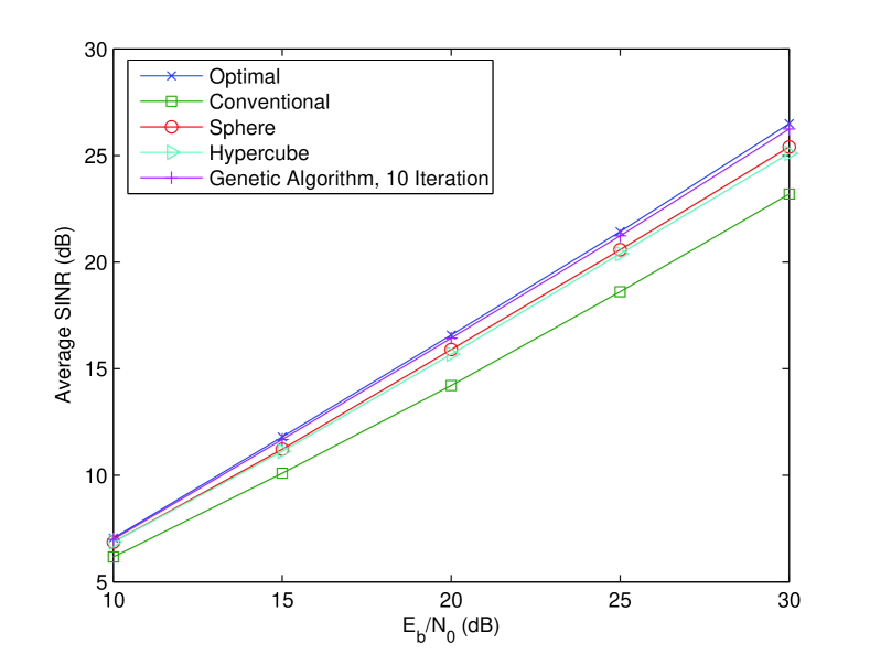
Figure 3: Average $\rm{SINR}$ versus $E_{b}/N_{0}$ for $M=5$ fingers, where $E_{b}$ is the bit energy. The channel has $L=15$ multipath components and the taps are exponentially decaying. The IR-UWB system has $N_{c}=20$ chips per frame and $N_{f}=1$ frame per symbol. There are $5$ equal energy users in the system and random TH and polarity codes are used.

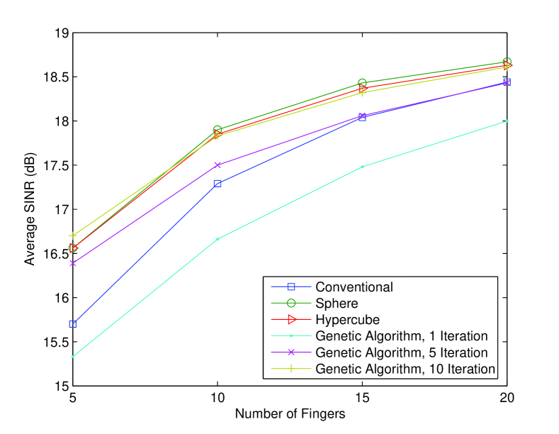
Figure 4: Average $\rm{SINR}$ versus number of fingers $M$, for $E_{b}/N_{0}=20$dB, $N_{c}=75$ and $L=50$. All the other parameters are the same as those for Figure 3.

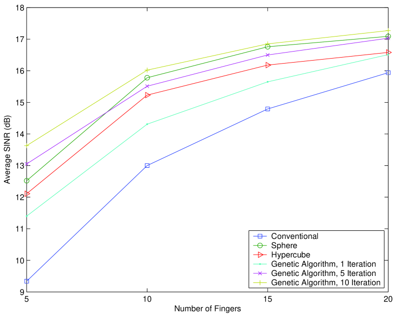
Figure 5: Average $\rm{SINR}$ versus number of fingers $M$. There are $10$ users with each interferer having $10$dB more power than the desired user. All the other parameters are the same as those for Figure 4.

References

- [1] U. S. Federal Communications Commission, FCC 02-48: First Report and Order.
- [2] M. Z. Win and R. A. Scholtz, “Impulse radio: How it works,” IEEE Communications Letters, 2(2): pp. 36-38, Feb. 1998.
- [3] M. Z. Win and R. A. Scholtz, “Ultra-wide bandwidth time-hopping spread-spectrum impulse radio for wireless multiple-access communications,” IEEE Transactions on Communications, vol. 48, pp. 679-691, April 2000.
- [4] F. Ramirez Mireless, “On the performance of ultra-wideband signals in Gaussian noise and dense multipath,” IEEE Transactions on Vehicular Technology, vol. 50, no. 1, pp. 244-249, Jan. 2001.
- [5] R. A. Scholtz, “Multiple access with time-hopping impulse modulation,” Proc. IEEE Military Communications Conference (MILCOM 1993), vol. 2, pp. 447-450, Boston, MA, Oct. 1993.
- [6] D. Cassioli, M. Z. Win and A. F. Molisch, “The ultra-wide bandwidth indoor channel: From statistical model to simulations,” IEEE Journal on Selected Areas in Communications, vol. 20, pp. 1247-1257, Aug. 2002.
- [7] D. Cassioli, M. Z. Win, F. Vatalaro and A. F. Molisch, “Performance of low-complexity RAKE reception in a realistic UWB channel,” Proc. IEEE International Conference on Communications (ICC 2002), vol. 2, pp. 763-767, New York, NY, April 28-May 2, 2002.
- [8] M. Z. Win and J. H. Winters, “Analysis of hybrid selection/maximal-ratio combining of diversity branches with unequal SNR in Rayleigh fading,” Proc. IEEE 49th Vehicular Technology Conference (VTC 1999-Spring), vol. 1, pp. 215-220, Houston, TX, May 16-20, 1999.
- [9] N. Kong and L. B. Milstein, “Combined average SNR of a generalized diversity selection combining scheme,” Proc. IEEE International Conference on Communications (ICC 1998), vol. 3, pp. 1556-1560, Atlanta, GA, June 7-11, 1998.
- [10] L. Yue, “Analysis of generalized selection combining techniques,” Proc. IEEE 51st Vehicular Technology Conference (VTC 2000-Spring), vol. 2, pp. 1191-1195, Tokyo, Japan, May 15-18, 2000.
- [11] Haichang Sui, E. Masry, B. D. Rao, Y. C. Yoon, “CDMA downlink chip-level MMSE equalization and finger placement,” Proc. Asilomar Conference on Signals, Systems and Computers, vol. 1, pp. 1161-1165, Pacific Grove, CA, Nov. 2003.
- [12] Haichang Sui, E. Masry, B. D. Rao, “RAKE finger placement for CDMA downlink equalization,” Proc. IEEE International Conference on Acoustics, Speech, and Signal Processing, vol.3, pp. iii/905-iii/908, Philadelphia, PA, March 2005.
- [13] Lin Zhiwei, A. B. Premkumar, A. S. Madhukumar, “Matching pursuit-based tap selection technique for UWB channel equalization,” IEEE Communications Letters, vol. 9, pp. 835-837, Sept. 2005.
- [14] E. Fishler and H. V. Poor, “On the tradeoff between two types of processing gain,” IEEE Transactions on Communications, vol. 53, no. 10, pp. 1744-1753, Oct. 2005.
- [15] S. Gezici, H. Kobayashi, H. V. Poor and A. F. Molisch, “Performance evaluation of impulse radio UWB systems with pulse-based polarity randomization in asynchronous multiuser environments,” Proc. IEEE Wireless Communications and Networking Conference (WCNC 2004), vol. 2, pp. 908-913, Atlanta, GA, March 2004.
- [16] Y.-P. Nakache and A. F. Molisch, “Spectral shape of UWB signals - Influence of modulation format, multiple access scheme and pulse shape,” Proc. IEEE 57th Vehicular Technology Conference, (VTC 2003-Spring), vol. 4, pp. 2510-2514, Jeju, Korea, April 2003.
- [17] S. Gezici, H. Kobayashi, H. V. Poor and A. F. Molisch, “Performance evaluation of impulse radio UWB systems with pulse-based polarity randomization,” IEEE Transactions on Signal Processing, vol. 53, no. 7, pp. 2537-2549, July 2005.
- [18] S. Gezici, H. Kobayashi, H. V. Poor, and A. F. Molisch, “Optimal and suboptimal linear receivers for time-hopping impulse radio systems,” Proc. IEEE Conference on Ultra Wideband Systems and Technologies (UWBST 2004), Kyoto, Japan, May 18-21, 2004.
- [19] A. F. Molisch, Y. P. Nakache, P. Orlik, J. Zhang, Y. Wu, S. Gezici, S. Y. Kung, H. Kobayashi, H. V. Poor, Y. G. Li, H. Sheng and A. Haimovich, “An efficient low-cost time-hopping impulse radio for high data rate transmission,” Proc. IEEE 6th International Symposium on Wireless Personal Multimedia Communications (WPMC 2003), Yokosuka, Kanagawa, Japan, Oct. 19-22, 2003.
- [20] S. Verdú. Multiuser Detection, Cambridge University Press, Cambridge, UK, 1998.
- [21] S. Boyd and L. Vandenberghe, Convex Optimization, Cambridge University Press, Cambridge, UK, 2004.
- [22] Y. Nesterov and A. Nemirovskii, Interior-Point Polynomial Methods in Convex Programming, Society for Industrial and Applied Mathematics Press, Philadelphia, PA, 1994.
- [23] R. L. Haupt and S. E. Haupt, Practical Genetic Algorithms, John Wiley & Sons Inc., New York, 1998.
- [24] D. E. Goldberg, Genetic Algorithms in Search, Optimization, and Machine Learning,Addison-Wesley, Reading, MA, 1989.
- [25] M. Mitchell, An Introduction to Genetic Algorithms, MIT Press, Cambridge, MA, 1996.
- [26] M. J. Juntti, T. Schlösser and J. O. Lilleberg, “Genetic algorithms for multiuser detection in synchronous CDMA,” Proc. IEEE International Symposium on Information Theory, p. 492, Ulm, Germany, June 29-July 4, 1997.
- [27] C. Ergün and K. Hacioglu, “Multiuser detection using a genetic algorithm in CDMA communications systems,” IEEE Transactions on Communications, vol. 48, no. 8, pp. 1374-1383, Aug. 2000.
- [28] K. Yen and L. Hanzo, “Genetic-algorithm-assisted multiuser detection in asynchronous CDMA communications,” IEEE Transactions on Vehicular Technology, vol. 53, no. 5, pp. 1413-1422, Sept. 2004.