Robust Distributed Source Coding

Abstract

We consider a distributed source coding system in which several observations are communicated to the decoder using limited transmission rate. The observations must be separately coded. We introduce a robust distributed coding scheme which flexibly trades off between system robustness and compression efficiency. The optimality of this coding scheme is proved for various special cases.

Index Terms—CEO problem, common information, distributed source coding, multiple descriptions.

I Introduction

There are many situations in which data collected at several sites must be transmitted to a common point for subsequent processing. Via clever encoding techniques, it is possible to capitalize on the correlation between data received at the various sites even though each encoder operates with no or only partial knowledge of the data received at the other sites. Slepian and Wolf [1] proved a coding theorem for two correlated memoryless sources with separate encoders. They dealt with the case where the decoder must reproduce two source outputs with arbitrary small error probability. Their results were extended to arbitrary number of discrete sources with ergodic memory and countably infinite alphabets by Cover [2]. Based on the results of Slepian and Wolf, Wyner and Ziv [3] extended rate-distortion theory to the case in which side information is present at the decoder. Berger [4] and Tung [5] generalized the Slepian-Wolf problem by considering general distortion criteria on the source reconstruction. The complete characterization of the rate-distortion region is unknown except for the special case where one of two source outputs must be reconstructed with an arbitrary small error probability and the other must have an average distortion smaller than a prescribed level [6]. Oohama [7] studied the rate-distortion region for correlated memoryless Gaussian sources and squared distortion measures. He demonstrated that the inner bound of the rate-distortion region obtained by Berger and Tung is partially tight in the Gaussian case. Viswanath [8] characterized the sum-rate distortion function of Gaussian multiterminal source coding problem for a class of quadratic distortion metrics. A closely related problem, called the remote source coding problem or the CEO problem, has been studied in [9, 10, 11, 12, 13]. Oohama [14] derived the sum-rate distortion function for the quadratic Gaussian CEO problem when there are infinite encoders and the SNRs at all the encoders are identical. It was observed by Chen et al. [15] that Oohama’s converse yields a tight upper bound on the sum-rate distortion function even when the number of encoders are finite. They also computed the achievable region for the general quadratic Gaussian CEO problem. Recently, Oohama [16] and Prabhakaran et al. [17] showed that this achievable region is indeed the rate-distortion region.

Another important class of source coding problems is called multiple description problem. In the multiple description problem, the total available bit rate is split between (say) two channels and either channel may be subject to failure. It is desired to allocate rate and coded representations between the two channels, such that if one channel fails, an adequate reconstruction of the source is possible, but if both channels are available, an improved reconstruction over the single-channel reception results. This problem was posed by Gersho, Witsenhausen, Wolf, Wyner, Ziv and Ozarow in 1979. Early contributions to this problem can be found in Witsenhausen [18], Wolf, Wyner and Ziv [19], Ozarow [20] and Witsenhausen and Wyner [21]. The first general result was El Gamal and Cover’s achievable region for two channels [22]. Ahlswede [23] showed that in the “no excess rate” case, El Gamal and Cover’s region is tight. Zhang and Berger [24] exhibit a simple counterexample that shows El Gamal and Cover’s region is not always tight in the case of an excess rate. Further results can be found in [25, 26, 27, 28, 29, 30, 31, 32].

Distributed source coding problems of the Slepian-Wolf type and its extensions emphasize the compression efficiency of coding system but ignore the system robustness. A distributed source coding scheme which is optimal in the sense of compression efficiency can be very sensitive to the encoder failure, i.e., the performance of the whole system may degenerate dramatically when one of the encoders is subject to a failure. On the other hand, multiple description problem does consider the system robustness. But it is essentially a centralized source coding problem whose coding schemes in general can not be applied in the distributed source coding scenario. So it is of interest to study robust distributed source coding scheme, which is able to trade off between two important parameters: system robustness and compression efficiency.

II System Model and Problem Formulation

Consider the distributed source coding system shown in Fig. 1. Let $\{X(t),Y_{1}(t),Y_{2}(t)\}_{t=1}^{\infty}$ be temporally memoryless source with instantaneous joint probability distribution $P(x,y_{1},y_{2})$ on $\mathcal{X}\times\mathcal{Y}_{1}\times\mathcal{Y}_{2}$, where $\mathcal{X}$ is the common alphabet of the random variables $X(t)$ for $t=1,2,\cdots$, $\mathcal{Y}_{i}\ (i=1,2)$ is the common alphabet of the random variables $Y_{i}(t)$ for $t=1,2,\cdots$. $\{X(t)\}_{t=1}^{\infty}$ is the target data sequence which can not be observed directly. Instead, two corrupted versions of $\{X(t)\}_{t=1}^{\infty}$, i.e., $\{Y_{1}(t)\}_{t=1}^{\infty}$ and $\{Y_{2}(t)\}_{t=1}^{\infty}$, are observed by encoder 1 and encoder 2 respectively. Encoder $i$ encodes a block $y_{i}^{n}=[y_{i}(1),\cdots,y_{i}(n)]$ of length $n$ from its observed data using a source code $c_{i}^{(n)}=f_{E,i}^{(n)}(y_{i}^{n})$ of rate $\frac{1}{n}\log|\mathcal{C}_{i}^{(n)}|$. Decoder $i$ reconstructs the target sequence $x^{n}=[x(1),\cdots,x(n)]$ by implementing a mapping $f^{(n)}_{D,i}:\ \mathcal{C}^{(n)}_{i}\rightarrow\mathcal{X}^{n},\quad i=1,2$. Decoder 3 reconstructs the target sequence $x^{n}=[x(1),\cdots,x(n)]$ by implementing a mapping $f^{(n)}_{D,3}:\ \mathcal{C}_{1}^{(n)}\times\mathcal{C}_{2}^{(n)}\rightarrow\mathcal{X}^{n}$.

\psfrag{x}[c]{$X$}\psfrag{y1}[c]{$Y_{1}$}\psfrag{y2}[c]{$Y_{2}$}\psfrag{en1}[c]{Encoder $1$}\psfrag{en2}[c]{Encoder $2$}\psfrag{de1}[c]{Decoder $1$}\psfrag{de2}[c]{Decoder $2$}\psfrag{de3}[c]{Decoder $3$}\psfrag{xhat1}[l]{$\hat{X}_{1}\sim D_{1}$}\psfrag{xhat2}[l]{$\hat{X}_{2}\sim D_{2}$}\psfrag{xhat3}[l]{$\hat{X}_{3}\sim D_{3}$}\psfrag{r1}[c]{$R_{1}$}\psfrag{r2}[c]{$R_{2}$}\includegraphics[scale={0.7}]{systemmodel1}

Figure 1: Model of robust distributed source coding system

Definition 1

The quintuple $(R_{1},R_{2},D_{1},D_{2},D_{3})$ is called achievable, if for any $\epsilon>0$, there exists an $n_{0}$ such that for all $n>n_{0}$ there exist encoders:

$$f_{E,i}^{(n)}:\mathcal{Y}_{i}^{n}\rightarrow\mathcal{C}_{i}^{(n)}\quad\log|\mathcal{C}_{i}^{(n)}|\leq n(R_{i}+\epsilon)\quad i=1,2$$

and decoders:

$$f^{(n)}_{D,i}:\ \mathcal{C}_{i}^{(n)}\rightarrow\mathcal{X}^{n}\quad i=1,2$$

$$f^{(n)}_{D,3}:\ \mathcal{C}_{1}^{(n)}\times\mathcal{C}_{2}^{(n)}\rightarrow\mathcal{X}^{n}$$

such that for $\hat{X}^{n}_{i}=f^{(n)}_{D,i}\left(f^{(n)}_{E,i}(Y^{n}_{i})\right),i=1,2$, and for $\hat{X}^{n}_{3}=f^{(n)}_{D,3}\left(f^{(n)}_{E,1}(Y^{n}_{1}),f^{(n)}_{E,2}(Y^{n}_{2})\right)$,

$$\frac{1}{n}\mathbb{E}\sum\limits_{t=1}^{n}d(X(t),\hat{X}_{i}(t))<D_{i}+\epsilon\quad i=1,2,3.$$

Here $d(\cdot,\cdot):\mathcal{X}\times\mathcal{X}\rightarrow[0,d_{\max}]$ is a given distortion measure.

Let $\mathcal{Q}$ denote the set of all achievable quintuples.

Remark:

1. Our model applies to many different scenarios such as the nonergodic link failures from some encoders to the decoder or the malfunction of some encoders;

2. We restrict our treatment to the case of two encoders just for simplifying the notations. Most of our results can be extended in a straightforward way to the case of arbitrary number of encoders;

Our model was first introduced by Ishwar et al. in [33]. An analogous problem called multilevel diversity coding has been studied in [34, 35, 36, 37]. But it is a centralized source coding problem since all the encoders have the same observation. A distributed version of multilevel diversity coding was introduced in [38], where only the case of lossless source coding was treated.

The rest of this paper is divided into four sections. Section III uses some examples to motivate the results. In Section IV, we first consider two different scenarios, namely, the centralized source coding and the distributed source coding, for which the corresponding coding schemes are established. Then we propose a unified approach by developing a coding scheme based on the idea of common information. In Section V, the case of correlated memoryless Gaussian observations and squared distortion measure is studied in detail. The inner bound and outer bound of the rate distortion region are established. We show that in various special cases the complete characterization of the rate distortion region is possible. Finally Section VI concludes the paper.

III Motivations and Examples

Let $D_{\max}=\min_{x_{0}\in\mathcal{X}}\mathbb{E}d(X,x_{0})$. Our problem reduces to the CEO problem if $\min(D_{1},D_{2})\geq D_{\max}$ and reduces the multiple description problem if there exist deterministic functions $f_{i}$ $(i=1,2)$ such that $X(t)=f_{i}(Y_{i}(t))$ with probability one for $t=1,2,\cdots$. So it is instructive to review the coding schemes for the CEO problem and multiple description problem.

For the CEO problem, the fidelity criterion is only imposed on the reconstruction of the target sequence at decoder 3. The largest known achievable rate distortion region for the CEO problem is the set of $(R_{1},R_{2},D_{3})$ for which there exist random variables $W_{1},W_{2}$ jointly distributed with the generic source variables $X,Y_{1}$ and $Y_{2}$ such that

• $W_{1}\rightarrow Y_{1}\rightarrow(X,Y_{2},W_{2})$ and $W_{2}\rightarrow Y_{2}\rightarrow(X,Y_{1},W_{1})$.

• $R_{1}\geq I(Y_{1};W_{1}|W_{2}),R_{2}\geq I(Y_{2};W_{2}|W_{1}),R_{1}+R_{2}\geq I(Y_{1},Y_{2};W_{1},W_{2})$.

• There exist a function $f:\mathcal{W}_{1}\times\mathcal{W}_{2}\rightarrow\mathcal{X}$ such that $\mathbb{E}d(X,{\hat{X}})\leq D$, where ${\hat{X}}=f(W_{1},W_{2})$.

The proof of the achievability of this rate distortion region is based on the idea of random binning. The main feature of the random binning coding scheme is outlined as follows:

There are many bins at each encoder and many codewords in each bin. Instead of directly sending the codeword, each encoder sends the index of bin which contains the codeword that this encoder wants to reveal to the decoder. Upon receiving the indices of bins from all the encoders, the decoder picks one codeword from each bin such that these codewords are jointly typical.

There are two important parameters for each encoder: the number of bins and the number of codewords. Roughly speaking, the number of bins determines the rate of the encoder while the number of codewords is associated with the description ability of the encoder. When the system is optimized in the sense of compression efficiency, the number of bins is minimized at each encoder if the number of its codewords is fixed (or equivalently, the number of codewords is maximized at each encoder if the number of its bins is fixed). Note: there exists a tradeoff between the maximum number of codewords at different encoders if the number of bins is fixed at each encoder (or equivalently, a tradeoff between the minimum number of bins at different encoders if the number of codewords is fixed at each encoder). But intuitively this optimization is achieved at the price of sacrificing the robustness of the whole system: if the decoder only receives the data from one of the encoders, then it may not be able to recover the correct codeword since the decoder only gets a bin index from one encoder and there are many codewords in that bin. Clearly, if there is only one codeword in each bin, then the decoder is able to recover the codeword as long as the bin index is received. Actually now the encoding scheme reduces to the conventional lossy source encoding and the joint decoding scheme becomes the separate decoding. In general, we can improve the robustness of the distributed source coding system by reducing the number of codewords in each bin, which is a way to trade the compression efficiency for the system robustness. This is essentially the main idea of the robust distributed source coding scheme proposed by Ishwar, Puri, Pradhan and Ramchandran [33], which we will refer to as the IPPR scheme. The achievable rate distortion region of IPPR scheme for our model is the set of $(R_{1},R_{2},D_{1},D_{2},D_{3})$ for which there exist random variables $W_{1},W_{2}$ jointly distributed with the generic source variables $X,Y_{1}$ and $Y_{2}$ such that

• $W_{1}\rightarrow Y_{1}\rightarrow(X,Y_{2},W_{2})$ and $W_{2}\rightarrow Y_{2}\rightarrow(X,Y_{1},W_{1})$.

• $R_{1}\geq I(Y_{1};W_{1}),R_{2}\geq I(Y_{2};W_{2})$.

• There exist functions $f_{i}:\mathcal{W}_{i}\rightarrow\mathcal{X}\quad(i=1,2)$, and $f_{3}:\mathcal{W}_{1}\times\mathcal{W}_{2}\rightarrow\mathcal{X}$ such that $\mathbb{E}d(X,{\hat{X}}_{i})\leq D_{i}\quad(i=1,2,3)$, where ${\hat{X}}_{1}=f_{1}(W_{1})$, ${\hat{X}}_{2}=f_{2}(W_{2})$ and ${\hat{X}}_{3}=f_{3}(W_{1},W_{2})$.

We need the following definition before discussing the properties of the IPPR scheme.

Definition 2

$$D^{*}_{1}(R_{1},R_{2})=\min\{D_{1}:(R_{1},R_{2},D_{1},D_{\max},D_{\max})\in\mathcal{Q}\},$$

$$D^{*}_{2}(R_{1},R_{2})=\min\{D_{2}:(R_{1},R_{2},D_{\max},D_{2},D_{\max})\in\mathcal{Q}\},$$

$$D^{*}_{3}(R_{1},R_{2})=\min\{D_{3}:(R_{1},R_{2},D_{\max},D_{\max},D_{3})\in\mathcal{Q}\}.$$

It is clear that $D^{*}_{1}(R_{1},R_{2})$ does not depend on $R_{2}$ and $D^{*}_{2}(R_{1},R_{2})$ does not depend on $R_{1}$, so we shall denote them by $D^{*}_{1}(R_{1})$ and $D^{*}_{2}(R_{2})$ respectively. $D^{*}_{1}(R_{1})$ and $D^{*}_{2}(R_{2})$ are essentially the distortion-rate functions with noisy observations [39][40], i.e.,

$$D^{*}_{i}(R_{i})=\min\limits_{\begin{subarray}{c}\hat{X}_{i}\in\mathcal{X}:X\rightarrow Y_{i}\rightarrow\hat{X}_{i}\\ I(Y_{i};\hat{X}_{i})\leq R_{i}\end{subarray}}\mathbb{E}d(X,\hat{X}_{i}),\quad i=1,2.$$

The IPPR scheme is of special interest in the sense that given rate tuple $(R_{1},R_{2})$, it can achieve $D^{*}_{1}(R_{1})$ and $D^{*}_{2}(R_{2})$ at decoder 1 and decoder 2 respectively as shown by the following argument:

Let $W^{*}_{1}(R_{1}),W^{*}_{2}(R_{2})\in\mathcal{X}$ be the random variables jointly distributed with $X,Y_{1}$ and $Y_{2}$ such that $W^{*}_{1}(R_{1})\rightarrow Y_{1}\rightarrow(X,Y_{2},W^{*}_{2}(R_{2}))$ and $W^{*}_{2}(R_{2})\rightarrow Y_{2}\rightarrow(X,Y_{1},W^{*}_{1}(R_{1}))$ with $I(Y_{i};W^{*}_{i}(R_{i}))\leq R_{i}$ and $\mathbb{E}d(X,W^{*}_{i}(R_{i}))=D^{*}_{i}(R_{i}),i=1,2$.

By the IPPR scheme, $(R_{1},R_{2},D^{*}_{1}(R_{1}),D^{*}_{2}(R_{2}),\min_{g:\mathcal{X}\times\mathcal{X}\rightarrow\mathcal{X}}Ed(X,g(W^{*}_{1}(R_{1}),W^{*}_{2}(R_{2}))))$ is achievable, where $\min_{g:\mathcal{X}\times\mathcal{X}\rightarrow\mathcal{X}}\mathbb{E}d(X,g(W^{*}_{1}(R_{1}),W^{*}_{2}(R_{2})))\leq\min(D^{*}_{1}(R_{1}),D^{*}_{2}(R_{2}))$ and the inequality is strict for most cases of interest.

Now we shall study the quadratic Gaussian case to get a concrete feeling about the IPPR scheme. Suppose $X\sim\mathcal{N}(0,\sigma^{2}_{X})$, $Y_{i}=X+N_{i}$, $N_{i}\sim\mathcal{N}(0,\sigma^{2}_{N_{i}})$, $i=1,2$. Here $X,N_{1}$ and $N_{2}$ are all independent. Let $W_{1}=Y_{1}+T_{1},W_{2}=Y_{2}+T_{2}$, where $T_{i}\sim\mathcal{N}(0,\sigma^{2}_{T_{i}})$, $i=1,2,$ are independent of $X,N_{1}$ and $N_{2}$.

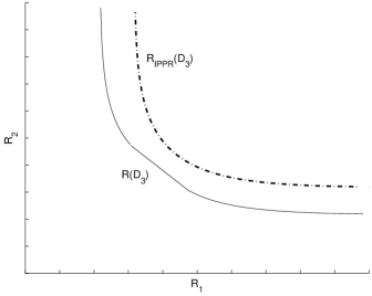
Figure 2: IPPR scheme

By the IPPR scheme, for any $(R_{1},R_{2})\in\mathcal{R}_{IPPR}(D_{1},D_{2},D_{3})$, we have $(R_{1},R_{2},D_{1},D_{2},D_{3})\in\mathcal{Q}$, where

$$\mathcal{R}_{IPPR}(D_{1},D_{2},D_{3})=\bigcup\limits_{(\sigma_{T_{1}}^{2},\sigma_{T_{2}}^{2})\in\Sigma^{\prime}(D_{1},D_{2},D_{3})}\mathcal{R}^{\prime}(\sigma_{T_{1}}^{2},\sigma_{T_{2}}^{2}),$$

$$\mathcal{R}^{\prime}(\sigma_{T_{1}}^{2},\sigma_{T_{2}}^{2})=\left\{(R_{1},R_{2}):R_{1}\geq I(Y_{1};W_{1})=\frac{1}{2}\log\frac{\sigma_{X}^{2}+\sigma_{N_{1}}^{2}+\sigma_{T_{1}}^{2}}{\sigma_{T_{1}}^{2}},\right.$$

$$\left.R_{2}\geq I(Y_{2};W_{2})=\frac{1}{2}\log\frac{\sigma_{X}^{2}+\sigma_{N_{2}}^{2}+\sigma_{T_{2}}^{2}}{\sigma_{T_{2}}^{2}}\right\}$$

and

$$\Sigma^{\prime}(D_{1},D_{2},D_{3})=\left\{(\sigma_{T_{1}}^{2},\sigma_{T_{2}}^{2}):D_{1}\geq\mathbb{E}(X-\mathbb{E}(X|W_{1}))^{2}=\left(\frac{1}{\sigma^{2}_{X}}+\frac{1}{\sigma_{N_{1}}^{2}+\sigma_{T_{1}}^{2}}\right)^{-1},\right.$$

$$D_{2}\geq\mathbb{E}(X-\mathbb{E}(X|W_{2}))^{2}=\left(\frac{1}{\sigma^{2}_{X}}+\frac{1}{\sigma_{N_{2}}^{2}+\sigma_{T_{2}}^{2}}\right)^{-1},$$

$$\left.D_{3}\geq\mathbb{E}(X-\mathbb{E}(X|W_{1},W_{2}))^{2}=\left(\frac{1}{\sigma^{2}_{X}}+\frac{1}{\sigma_{N_{1}}^{2}+\sigma_{T_{1}}^{2}}+\frac{1}{\sigma_{N_{2}}^{2}+\sigma_{T_{2}}^{2}}\right)^{-1}\right\}.$$

It was computed in [15] that

$$R(D,\sigma^{2}_{N})=\frac{1}{2}\log\frac{\sigma_{X}^{4}}{D\sigma_{X}^{2}-\sigma_{X}^{2}\sigma_{N}^{2}+D\sigma_{N}^{2}},$$

where $R(D,\sigma^{2}_{N})$ the sum-rate distortion function of the one-encoder quadratic Gaussian CEO problem. So we have

$$D^{*}_{i}(R_{i})=\frac{\sigma^{4}_{X}\exp(-2R_{i})+\sigma^{2}_{X}\sigma^{2}_{N_{i}}}{\sigma^{2}_{X}+\sigma^{2}_{N_{i}}},\quad i=1,2.$$

It is easy to check that $\left(R_{1},R_{2}\right)\in\mathcal{R}_{IPPR}(D^{*}_{1}(R_{1})$,$D^{*}_{2}(R_{2}),D_{3})$ given $D_{3}\geq(1/{D^{*}_{1}(R_{1})}+1/{D^{*}_{2}(R_{2})}-1/{\sigma_{X}^{2}})^{-1}$. Hence IPPR scheme can indeed achieve $D^{*}_{1}(R_{1})$ and $D^{*}_{2}(R_{2})$ at decoder 1 and decoder 2 respectively in the quadratic Gaussian case.

Let $\mathcal{R}(D_{3})=\left\{(R_{1},R_{2}):(R_{1},R_{2},\sigma^{2}_{X},\sigma^{2}_{X},D_{3})\in\mathcal{Q}\right\}$. It was shown in [16, 17] that

$$\mathcal{R}(D_{3})=\bigcup\limits_{(\sigma_{T_{1}}^{2},\sigma_{T_{2}}^{2})\in\Sigma^{\prime\prime}(D_{3})}\mathcal{R}^{\prime\prime}(\sigma_{T_{1}}^{2},\sigma_{T_{2}}^{2}),$$

where

$$\mathcal{R}^{\prime\prime}(\sigma_{T_{1}}^{2},\sigma_{T_{2}}^{2})=\left\{(R_{1},R_{2}):R_{1}\geq I(Y_{1};W_{1}|W_{2})=\frac{1}{2}\log\frac{(\sigma_{X}^{2}+\sigma_{N_{1}}^{2}+\sigma_{T_{1}}^{2})(\sigma_{X}^{2}+\sigma_{N_{2}}^{2}+\sigma_{T_{2}}^{2})-\sigma_{X}^{4}}{\sigma_{X}^{2}\sigma_{T_{1}}^{2}+\sigma_{N_{2}}^{2}\sigma_{T_{1}}^{2}+\sigma_{T_{1}}^{2}\sigma_{T_{2}}^{2}}\right.,$$

$$R_{2}\geq I(Y_{2};W_{2}|W_{1})=\frac{1}{2}\log\frac{(\sigma_{X}^{2}+\sigma_{N_{1}}^{2}+\sigma_{T_{1}}^{2})(\sigma_{X}^{2}+\sigma_{N_{2}}^{2}+\sigma_{T_{2}}^{2})-\sigma_{X}^{4}}{\sigma_{X}^{2}\sigma_{T_{2}}^{2}+\sigma_{N_{1}}^{2}\sigma_{T_{2}}^{2}+\sigma_{T_{1}}^{2}\sigma_{T_{2}}^{2}},$$

$$\left.R_{1}+R_{2}\geq I(Y_{1},Y_{2};W_{1},W_{2})=\frac{1}{2}\log\frac{(\sigma_{X}^{2}+\sigma_{N_{1}}^{2}+\sigma_{T_{1}}^{2})(\sigma_{X}^{2}+\sigma_{N_{2}}^{2}+\sigma_{T_{2}}^{2})-\sigma_{X}^{4}}{\sigma_{T_{1}}^{2}\sigma_{T_{2}}^{2}}\right\}$$

and

$$\Sigma^{\prime\prime}(D_{3})=\left\{(\sigma_{T_{1}}^{2},\sigma_{T_{2}}^{2}):D_{3}\geq\mathbb{E}(X-\mathbb{E}(X|W_{1},W_{2}))^{2}=\left(\frac{1}{\sigma^{2}_{X}}+\frac{1}{\sigma_{N_{1}}^{2}+\sigma_{T_{1}}^{2}}+\frac{1}{\sigma_{N_{2}}^{2}+\sigma_{T_{2}}^{2}}\right)^{-1}\right\}.$$

Let $\mathcal{R}_{IPPR}(D_{3})=\mathcal{R}_{IPPR}(\sigma^{2}_{X},\sigma^{2}_{X},D_{3})$. For comparison, we plot $\mathcal{R}_{IPPR}(D_{3})$ and $\mathcal{R}(D_{3})$ in Fig.2. It’s clear that $\mathcal{R}_{IPPR}(D_{3})\subsetneqq\mathcal{R}(D_{3})$. A natural question is to ask whether it is still possible to achieve not only $D_{3}$ but also nontrivial $D_{1}$ and $D_{2}$ when the system is operated in $\mathcal{R}(D_{3})\cap\mathcal{R}_{IPPR}^{c}(D_{3})$.

It has been shown in [8][15] that $\mathcal{R}^{\prime\prime}(\sigma_{T_{1}}^{2},\sigma_{T_{2}}^{2})$ is a contra-polymatroid. Its typical shape is plotted in Fig.3. The two vertices $E_{1}$ and $E_{2}$ of $\mathcal{R}^{\prime\prime}(\sigma_{T_{1}}^{2},\sigma_{T_{2}}^{2})$ are of special importance, where

$$E_{1} = \left(I(Y_{1};W_{1}),I(Y_{2};W_{2}|W_{1})\right)$$

$$= \left(\frac{1}{2}\log\frac{\sigma_{X}^{2}+\sigma_{N_{1}}^{2}+\sigma_{T_{1}}^{2}}{\sigma_{T_{1}}^{2}},\frac{1}{2}\log\frac{(\sigma_{X}^{2}+\sigma_{N_{1}}^{2}+\sigma_{T_{1}}^{2})(\sigma_{X}^{2}+\sigma_{N_{2}}^{2}+\sigma_{T_{2}}^{2})-\sigma_{X}^{4}}{\sigma_{X}^{2}\sigma_{T_{1}}^{2}+\sigma_{N_{2}}^{2}\sigma_{T_{1}}^{2}+\sigma_{T_{1}}^{2}\sigma_{T_{2}}^{2}}\right),$$

$$E_{2} = \left(I(Y_{1};W_{1}|W_{2}),I(Y_{2};W_{2})\right)$$

$$= \left(\frac{1}{2}\log\frac{(\sigma_{X}^{2}+\sigma_{N_{1}}^{2}+\sigma_{T_{1}}^{2})(\sigma_{X}^{2}+\sigma_{N_{2}}^{2}+\sigma_{T_{2}}^{2})-\sigma_{X}^{4}}{\sigma_{X}^{2}\sigma_{T_{2}}^{2}+\sigma_{N_{1}}^{2}\sigma_{T_{2}}^{2}+\sigma_{T_{1}}^{2}\sigma_{T_{2}}^{2}},\frac{1}{2}\log\frac{\sigma_{X}^{2}+\sigma_{N_{2}}^{2}+\sigma_{T_{2}}^{2}}{\sigma_{T_{2}}^{2}}\right).$$

Roughly speaking, the operational meaning for $E_{1}$ is that encoder 1 employs the conventional lossy source coding and encoder 2 does the Wyner-Ziv coding; while for $E_{2}$, encoder 2 employs the conventional lossy source coding and encoder 1 does the Wyner-Ziv coding. The Wyner-Ziv coding requires random binning scheme but the conventional lossy source coding does not. So when the system is operated at $E_{i}$ $(i=1,2)$, the decoder $i$ can decode the data sent by encoder $i$ and achieve

$$D_{i}=\mathbb{E}(X-\mathbb{E}(X|W_{1}))^{2}=\left(\frac{1}{\sigma^{2}_{X}}+\frac{1}{\sigma^{2}_{N_{i}}+\sigma^{2}_{T_{i}}}\right)^{-1}.$$ (1)

Furthermore, for vertex $E_{i}$, we have

$$R_{i}=I(Y_{i};W_{i})=\frac{1}{2}\log\left(\frac{\sigma_{X}^{2}+\sigma_{N_{1}}^{2}+\sigma_{T_{1}}^{2}}{{\sigma_{T_{1}}^{2}}}\right).$$ (2)

Combining (1) and (2), we get $R_{i}=R(D_{i},\sigma^{2}_{N_{i}})$. That is to say, the system can achieve $D^{*}_{i}(R_{i})$ at decoder $i$ when it is operated at $E_{i}$, $i=1,2$. As shown in Fig. 3, $\mathcal{R}(D_{3})$ is the union of $\mathcal{R}^{\prime\prime}(\sigma_{T_{1}}^{2},\sigma_{T_{2}}^{2})$. The boundary of $\mathcal{R}(D_{3})$ can be divided into three pieces: $A,B$ and $C$. Each point on $A$ corresponds to vertex $E_{1}$ of $\mathcal{R}^{\prime\prime}(\sigma_{T_{1}}^{2},\sigma_{T_{2}}^{2})$ for some $(\sigma_{T_{1}}^{2},\sigma_{T_{2}}^{2})$. Each point on $C$ corresponds to vertex $E_{2}$ of $\mathcal{R}^{\prime\prime}(\sigma_{T_{1}}^{2},\sigma_{T_{2}}^{2})$ for some $(\sigma_{T_{1}}^{2},\sigma_{T_{2}}^{2})$. So when the system is operated at $(R_{1},R_{2})$ on curve $A$, it can achieve $D^{*}_{1}(R_{1})$ at decoder 1 and at the same time achieve $D^{*}_{3}(R_{1},R_{2})$ at decoder 3. Curve $C$ is similar to Curve $A$ with the only difference that now the system can achieve $D^{*}_{2}(R_{2})$ at decoder 2. This observation immediately yields the following partial characterization of $\mathcal{Q}$:

Let $D_{i,\min}=\mathbb{E}(X-\mathbb{E}(X|Y_{i})))^{2}=(1/\sigma_{X}^{2}+1/\sigma_{N_{i}}^{2})^{-1}$, $i=1,2$, and $D_{3,\min}=\mathbb{E}(X-\mathbb{E}(X|Y_{1},Y_{2})))^{2}=(1/\sigma_{X}^{2}+1/\sigma_{N_{1}}^{2}+1/\sigma_{N_{1}}^{2})^{-1}$.

For any $D_{3}\in[D_{3,\min},\sigma^{2}_{X}]$, let

$$\tilde{\sigma}_{T_{1}}^{2}=\left\{\begin{array}[]{ll}\left(\frac{\sigma_{N_{1}}^{2}}{D_{3,\min}}-\frac{\sigma_{N_{1}}^{2}}{D_{3}}\right)\left(\frac{1}{\sigma_{N_{1}}^{2}}-\frac{1}{D_{2,\min}}+\frac{1}{D_{3}}\right)^{-1},\hskip 21.68121pt\frac{2}{\max(\sigma^{2}_{N_{1}},\sigma^{2}_{N_{2}})}+\frac{1}{D_{3}}-\frac{1}{D_{3,\min}}\geq 0\\ \left(\frac{\sigma_{N_{1}}^{2}}{D_{1,\min}}-\frac{\sigma_{N_{1}}^{2}}{D_{3}}\right)\left(\frac{1}{D_{3}}-\frac{1}{\sigma_{X}^{2}}\right)^{-1},\hskip 36.135pt\frac{2}{\max(\sigma^{2}_{N_{1}},\sigma^{2}_{N_{2}})}+\frac{1}{D_{3}}-\frac{1}{D_{3,\min}}<0\mbox{ and }\sigma^{2}_{N_{1}}<\sigma^{2}_{N_{2}}\\ \infty,\hskip 202.35622pt\mbox{otherwise},\\ \end{array}\right.$$

$$\tilde{\sigma}_{T_{2}}^{2}=\left\{\begin{array}[]{ll}\left(\frac{\sigma_{N_{2}}^{2}}{D_{3,\min}}-\frac{\sigma_{N_{2}}^{2}}{D_{3}}\right)\left(\frac{1}{\sigma_{N_{2}}^{2}}-\frac{1}{D_{1,\min}}+\frac{1}{D_{3}}\right)^{-1},\hskip 21.68121pt\frac{2}{\max(\sigma^{2}_{N_{1}},\sigma^{2}_{N_{2}})}+\frac{1}{D_{3}}-\frac{1}{D_{3,min}}\geq 0\\ \left(\frac{\sigma_{N_{2}}^{2}}{D_{2,\min}}-\frac{\sigma_{N_{2}}^{2}}{D_{3}}\right)\left(\frac{1}{D_{3}}-\frac{1}{\sigma_{X}^{2}}\right)^{-1},\hskip 36.135pt\frac{2}{\max(\sigma^{2}_{N_{1}},\sigma^{2}_{N_{2}})}+\frac{1}{D_{3}}-\frac{1}{D_{3,\min}}<0\mbox{ and }\sigma^{2}_{N_{1}}>\sigma^{2}_{N_{2}}\\ \infty,\hskip 202.35622pt\mbox{otherwise}.\end{array}\right.$$

We have

• For any $D_{1}\in[D_{1,\min},\sigma_{X}^{2}(\sigma_{N_{1}}^{2}+\tilde{\sigma}_{T_{1}}^{2})/(\sigma_{X}^{2}+\sigma_{N_{1}}^{2}+\tilde{\sigma}_{T_{1}}^{2})]$,

  $$\left\{(R_{1},R_{2}):(R_{1},R_{2},D_{1},\sigma^{2}_{X},D_{3})\in\mathcal{Q}\right\}=\left\{(R_{1},R_{2}):(R_{1},R_{2})\in\mathcal{R}(D_{3}),R_{1}\geq R(D_{1},\sigma_{N_{1}}^{2})\right\}.$$

• For any $D_{2}\in[D_{2,\min},\sigma_{X}^{2}(\sigma_{N_{2}}^{2}+\tilde{\sigma}_{T_{2}}^{2})/(\sigma_{X}^{2}+\sigma_{N_{2}}^{2}+\tilde{\sigma}_{T_{2}}^{2})]$,

  $$\left\{(R_{1},R_{2}):(R_{1},R_{2},\sigma^{2}_{X},D_{2},D_{3})\in\mathcal{Q}\right\}=\left\{(R_{1},R_{2}):(R_{1},R_{2})\in\mathcal{R}(D_{3}),R_{2}\geq R(D_{2},\sigma_{N_{2}}^{2})\right\}.$$

• For any $D_{1}\in[D_{1,\min},\sigma_{X}^{2}(\sigma_{N_{1}}^{2}+\tilde{\sigma}_{T_{1}}^{2})/(\sigma_{X}^{2}+\sigma_{N_{1}}^{2}+\tilde{\sigma}_{T_{1}}^{2})]$ and $D_{2}\in[D_{2,\min},\sigma_{X}^{2}(\sigma_{N_{2}}^{2}+\tilde{\sigma}_{T_{2}}^{2})/(\sigma_{X}^{2}+\sigma_{N_{2}}^{2}+\tilde{\sigma}_{T_{2}}^{2})]$,

  $$\left\{(R_{1},R_{2}):(R_{1},R_{2},D_{1},D_{2},D_{3})\in\mathcal{Q}\right\}=\left\{(R_{1},R_{2}):R_{i}\geq R(D_{i},\sigma_{N_{i}}^{2}),i=1,2\right\}.$$

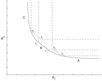
Figure 3: The boundary of $\mathcal{R}(D_{3})$

Since any rate tuple $(R_{1},R_{2})$ on line segment $B$ can be viewed as the timesharing of $F_{1}$ and $F_{2}$, it implies that when the system is operated on line segment $B$, it can achieve $D^{*}_{3}(R_{1},R_{2})$ at decoder 3 and at the same time achieve nontrivial $D_{1}$ and $D_{2}$ at decoder 1 and decoder 2, respectively.

The IPPR scheme can achieve $D^{*}_{1}(R_{1})$ and $D^{*}_{2}(R_{2})$ at decoder 1 and decoder 2 respectively, but can not achieve $D^{*}_{3}(R_{1},R_{3})$ at decoder 3 in general The coding scheme we described above can achieve $D^{*}_{3}(R_{1},R_{2})$ at decoder 3 (at least in the case of quadratic Gaussian CEO problem) and at the same time achieve nontrivial $D_{1}$ and $D_{2}$ at decoder 1 and decoder 2, but in general we have $D_{i}>D^{*}_{i}(R_{i})$, $i=1,2$. We will see that these are two extremes and there exist many other schemes in between.

Like the CEO problem, the multiple description problem has been studied for years and many multiple description coding schemes have been proposed. Here we outline the common feature of the existing multiple description coding schemes: encoder $i$ $(i=1,2)$, instead of sending an index $C^{(n)}_{i}$, sends a vector, say $(C^{(n)}_{i,1},C^{(n)}_{i,2})$; decoder $i$ $(i=1,2)$ can only decode the $C^{(n)}_{i,1}-$part; decoder 3 can decode both $(C^{(n)}_{1,1},C^{(n)}_{1,2})$ and $(C^{(n)}_{2,1},C^{(n)}_{2,2})$. Clearly, this idea is also applicable in the distributed source coding. Moreover, we can see that the IPPR scheme corresponds to the case where $C^{(n)}_{1,2}$ and $C^{(n)}_{2,2}$ are constants.

In the next section, we propose a robust distributed coding scheme by combining the random binning technique and the ideas from the multiple description coding.

IV Main Theorems

IV-A An Achievable Rate-Distortion Region

Theorem 1

$(R_{1},R_{2},D_{1},D_{2},D_{3})$ is achievable, if there exist random variables $(U_{1},U_{2},W_{1},W_{2})$ jointly distributed with the generic source variables $(X,Y_{1},Y_{2})$ such that the following properties are satisfied:

• $(U_{1},W_{1})\rightarrow Y_{1}\rightarrow(X,Y_{2},U_{2},W_{2})$ and $(U_{2},W_{2})\rightarrow Y_{2}\rightarrow(X,Y_{1},U_{1},W_{1})$.

• $(R_{1},R_{2})\in\mathcal{R}(U_{1},U_{2},W_{1},W_{2})$, where

  $$\mathcal{R}(U_{1},U_{2},W_{1},W_{2})=\left\{(R_{1},R_{2}):R_{1}\geq I(Y_{1};U_{1})+I(Y_{1};W_{1}|U_{1},U_{2},W_{2}),\right.$$

  $$R_{2}\geq I(Y_{2};U_{2})+I(Y_{2};W_{2}|U_{1},U_{2},W_{1}),$$

  $$\left.R_{1}+R_{2}\geq I(Y_{1};U_{1})+I(Y_{2};U_{2})+I(Y_{1},Y_{2};W_{1},W_{2}|U_{1},U_{2})\right\}.$$

• There exist functions $f_{i}:\mathcal{W}_{i}\rightarrow\mathcal{X}\ (i=1,2)$ and $f_{3}:\mathcal{U}_{1}\times\mathcal{W}_{1}\times\mathcal{U}_{2}\times\mathcal{W}_{2}\rightarrow\mathcal{X}$ such that $\mathbb{E}d(X,{\hat{X}}_{i})\leq D_{i},i=1,2,3$, where ${\hat{X}}_{1}=f_{1}(U_{1})$, ${\hat{X}}_{2}=f_{2}(U_{2})$ and ${\hat{X}}_{3}=f_{3}(U_{1},W_{1},U_{2},W_{2})$.

If $\mathcal{C}$ denotes the set of these achievable quintuples, then time sharing yields that $\mathcal{Q}_{in}\triangleq conv(\mathcal{C})$ is also an achievable region.

Proof:

See Appendix I. ∎

Remark:

1. Cardinality bound: By invoking the support lemma [41, pp.310], $\mathcal{U}_{1}$ must have $|\mathcal{Y}_{1}|-1$ letters to preserve the probability distribution $P(y_{1})$ and 5 more to preserve $I(Y_{1};U_{1})+I(Y_{1};W_{1}|U_{1},U_{2},W_{2})$, $I(Y_{2};W_{2}|U_{1},U_{2},W_{1})$, $I(Y_{1};U_{1})+I(Y_{1},Y_{2};W_{1},W_{2}|U_{1},U_{2})$, $D_{1}$ and $D_{3}$, so $|\mathcal{U}_{1}|=|\mathcal{Y}_{1}|+4$ suffices. $\mathcal{W}_{1}$ must have $|\mathcal{Y}_{1}||\mathcal{U}_{1}|-1$ letters to preserve the probability distribution $P(y_{1},u_{1})$ and 4 more to preserve $I(Y_{1};W_{1}|U_{1},U_{2},W_{2})$, $I(Y_{2};W_{2}|U_{1},U_{2},W_{1})$, $I(Y_{1},Y_{2};W_{1},W_{2}|U_{1},U_{2})$ and $D_{3}$. Thus it suffices to have $|\mathcal{W}_{1}|=|\mathcal{Y}_{1}||\mathcal{U}_{1}|-1+4=|\mathcal{Y}_{1}|^{2}+4|\mathcal{Y}_{1}|+3$. Similarly, we have $|\mathcal{U}_{2}|=|\mathcal{Y}_{2}|+4$, $|\mathcal{W}_{2}|=|\mathcal{Y}_{2}|^{2}+4|\mathcal{Y}_{2}|+3$.

2. It’s easy to check that $\mathcal{R}(U_{1},U_{2},W_{1},W_{2})$ is a contra-polymatroid. See [42] for the defintion of contra-polymatroid and [8, 15, 17, 43, 44, 45] for its applications in information theory.

3. Let $W^{\prime}_{i}=(U_{i},W_{i})$, $i=1,2$. It’s easy to check that $\mathcal{R}(U_{1},U_{2},W^{\prime}_{1},W^{\prime}_{2})=\mathcal{R}(U_{1},U_{2},W_{1},W_{2})$ and $\hat{X}_{3}=f_{3}(U_{1},U_{2},W_{1},W_{2})=f^{\prime}_{3}(W^{\prime}_{1},W^{\prime}_{2})$. So there is no loss of generality to assume $U_{i}\rightarrow W_{i}\rightarrow Y_{i}$ and define $f_{3}$ on $\mathcal{W}_{1}\times\mathcal{W}_{2}$.

4. Let $\mathcal{R}^{\prime}(U_{1},U_{2},W_{1},W_{2})=\{(R_{1},R_{2}):R_{1}\geq I(Y_{1};U_{1})+I(Y_{1};W_{1}|U_{1},U_{2},W_{2}),R_{2}\geq I(Y_{2};U_{2})+I(Y_{2};W_{2}|U_{1},U_{2})\}$, $\mathcal{R}^{\prime\prime}(U_{1},U_{2},W_{1},W_{2})=\{(R_{1},R_{2}):R_{1}\geq I(Y_{1};U_{1})+I(Y_{1};W_{1}|U_{1},U_{2}),R_{2}\geq I(Y_{2};U_{2})+I(Y_{2};W_{2}|U_{1},U_{2},W_{1})\}$. Since $conv(\mathcal{R}^{\prime}(U_{1},U_{2},W_{1},W_{2})\cup\mathcal{R}^{\prime\prime}(U_{1},U_{2},W_{1},W_{2}))=\mathcal{R}(U_{1},U_{2},W_{1},W_{2})$, we can let $(R_{1},R_{2})\in\mathcal{R}^{\prime}(U_{1},U_{2},W_{1},W_{2})\cup\mathcal{R}^{\prime\prime}(U_{1},U_{2},W_{1},W_{2})$ in property (ii) without affecting $\mathcal{Q}_{in}$.

A counter example constructed by Körner and Marton [46] shows that $conv(\mathcal{C})\subsetneqq\mathcal{Q}$ in general. Actually even some special cases of our problem such as the multiple description problem and the CEO problem are the open problems of long standing. But for the following case, a stronger assertion can be made.

Corollary 1

For any $D_{1}$ and $D_{3}$, we have $\min\{R_{1}:\exists R_{2}\mbox{ such that }(R_{1},R_{2},D_{1},D_{\max},D_{3})\in\mathcal{Q}\}=\min[I(Y_{1};U_{1})+I(Y_{1};W_{1}|Y_{2},U_{1})]$, where the minimization is over the set of all random variables $(U_{1},W_{1})$ jointly distributed with the generic source variables $(X,Y_{1},Y_{2})$ such that the following conditions are satisfied:

• $(U_{1},W_{1})\rightarrow Y_{1}\rightarrow(X,Y_{2})$.

• There exist functions $f:\mathcal{U}_{1}\rightarrow\mathcal{X}$, $g:\mathcal{U}_{1}\times\mathcal{W}_{1}\times\mathcal{Y}_{2}\rightarrow\mathcal{X}$ such that $\mathbb{E}d(X,f(U_{1}))\leq D_{1}$, $\mathbb{E}d(X,g(Y_{2},U_{1},W_{1}))\leq D_{3}$.

• $|\mathcal{U}_{1}|=|\mathcal{Y}_{1}|+2$, $|\mathcal{W}_{1}|=(|\mathcal{Y}_{1}|+1)^{2}$.

Remark: For the same reason as before, there is no loss of optimality to assume $U_{1}\rightarrow W_{1}\rightarrow Y_{1}$ and define $g$ on $\mathcal{W}_{1}\times\mathcal{Y}_{2}$.

Proof:

Since here we are only interested in minimizing $R_{1}$ under the distortion constraints $D_{1}$ and $D_{3}$, there is no loss of generality to assume that $R_{2}$ is large enough so that $\{Y_{2}(t)\}_{t=1}^{\infty}$ can be recovered losslessly at decoder 3. In the case, our problem becomes the “noisy” Heegard-Berger problem. Its direct coding theorem can be easily reduced from Theorem 1 while the converse coding theorem can be proved along the same line as the converse in [47]. ∎

IV-B Distributed Source Coding with Identical Encoders

For many applications, it is preferable to have encoders with identical functionalities. It is thus interesting to study the distributed source coding system with identical encoders. In order to have $f^{(n)}_{E,1}=f^{(n)}_{E,2}$, two necessary conditions are required: (1) $R_{1}=R_{2}$, (2) $\mathcal{Y}_{1}=\mathcal{Y}_{2}$. We need the first condition to guarantee the range cardinalities of $f^{(n)}_{E,1}$ and $f^{(n)}_{E,2}$ are the same, and the second condition to guarantee these two encoding functions are defined on the same domain. Without loss of generality, we can assume the second condition is satisfied since we can let $\mathcal{Y}=\mathcal{Y}_{1}\cup\mathcal{Y}_{2}$ and extend the probability distribution $P(x,y_{1},y_{2})$ to be defined on $\mathcal{X}\times\mathcal{Y}\times\mathcal{Y}$.

But even with these two conditions, it can not be guaranteed that the resulting encoding functions $f^{(n)}_{E,1}$ and $f^{(n)}_{E,2}$ in Theorem 1 are identical. Intuitively, in order to minimize the distortion $D_{3}$ for the fixed rate constraints, the $f^{(n)}_{E,1}$ and $f^{(n)}_{E,2}$ generated by the random coding argument in the proof of Theorem 1 should be complementary to each other instead of being identical. We may imagine that a restriction on the identicalness of $f^{(n)}_{E,1}$ and $f^{(n)}_{E,2}$ may incur performance loss. But we will show that for many cases, no performance degradation will be caused. Firstly, we need a formal definition.

Definition 3

The quadruple $(R,D_{1},D_{2},D_{3})$ is called achievable with identical encoders, if for any $\epsilon>0$, there exists an $n_{0}$ such that for all $n>n_{0}$ there exist an encoding function:

$$f_{E}^{(n)}:\mathcal{Y}^{n}\rightarrow\mathcal{C}^{(n)}\quad\log|\mathcal{C}^{(n)}|\leq n(R+\epsilon)$$

and decoders:

$$f^{(n)}_{D,i}:\ \mathcal{C}^{(n)}\rightarrow\mathcal{X}^{n}\quad i=1,2$$

$$f^{(n)}_{D,3}:\ \mathcal{C}^{(n)}\times\mathcal{C}^{(n)}\rightarrow\mathcal{X}^{n}$$

such that for $\hat{X}^{n}_{i}=f^{(n)}_{D,i}(f^{(n)}_{E}(Y^{n}_{i})),i=1,2$, and for $\hat{X}^{n}_{3}=f^{(n)}_{D,3}(f^{(n)}_{E}(Y^{n}_{1}),f^{(n)}_{E}(Y^{n}_{2}))$,

$$\frac{1}{n}E\sum\limits_{t=1}^{n}d(X(t),\hat{X}_{i}(t))<D_{i}+\epsilon\quad i=1,2,3.$$

Let $\widetilde{\mathcal{Q}}$ denote the set of all achievable quadruples.

It is clear by definition that $\min\{R:(R,D_{1},D_{2},D_{3})\in\widetilde{\mathcal{Q}}\}$ is lower bounded by $\min\{R:(R,R,D_{1},D_{2},D_{3})\in\mathcal{Q}\}$. The following theorem provides an upper bound on $\min\{R:(R,D_{1},D_{2},D_{3})\in\widetilde{\mathcal{Q}}\}$.

Theorem 2

For any feasible $(D_{1},D_{2},D_{3})$,

• $\min\{R:(R,D_{1},D_{2},D_{3})\in\widetilde{\mathcal{Q}}\}\leq\min(\min\{R_{1}+R_{2}:(R_{1},R_{2},D_{1},D_{2},D_{3})\in\mathcal{Q}\},H_{\max})$, where $H_{\max}=\max(H(Y_{1}),H(Y_{2}))$.

• $\min\{R:(R,D_{1},D_{2},D_{3})\in\widetilde{\mathcal{Q}}\}=\min\{R:(R,R,D_{1},D_{2},D_{3})\in\mathcal{Q}\}$ if $P(Y_{1}=y)\neq P(Y_{2}=y)$ for some $y\in\mathcal{Y}$.

Proof:

(1) For any $f^{(n)}_{E,1}$ and $f^{(n)}_{E,2}$ , let $f^{(n)}_{E}=(f^{(n)}_{E,1},f^{(n)}_{E,2})$. So if $|f^{(n)}_{E,1}|=2^{nR_{1}},|f^{(n)}_{E,2}|=2^{nR_{2}}$, then we have $|f^{(n)}_{E}|\leq 2^{n(R_{1}+R_{2})}$. It’s clear that if we replace both $f^{(n)}_{E,1}$ and $f^{(n)}_{E,2}$ by $f^{(n)}_{E}$, no additional estimation distortion will be incurred. Hence we have $\min\{R:(R,D_{1},D_{2},D_{3})\in\widetilde{\mathcal{Q}}\}\leq\min\{R_{1}+R_{2}:(R_{1},R_{2},D_{1},D_{2},D_{3})\in\mathcal{Q}\}$.

On the other hand, for any $\epsilon>0$, we can find a universal lossless source encoding function with rate $R\leq H_{\max}+\epsilon$ that works for both $\{Y_{1}(t)\}_{t=1}^{\infty}$ and $\{Y_{2}(t)\}_{t=1}^{\infty}$. This yields $\min\{R:(R,D_{1},D_{2},D_{3})\in\widetilde{\mathcal{Q}}\}\leq H_{\max}$.

(2) The above proof essentially constructed a common encoder by combining two encoding functions. We now show that if $P(Y_{1}=y)\neq P(Y_{2}=y)$ for some $y\in\mathcal{Y}$, i.e., $\{Y_{1}(t)\}_{t=1}^{\infty}$ and $\{Y_{2}(t)\}_{t=1}^{\infty}$ are distinguishable, we can combine two encoding functions in a more efficient way.

For $\delta>$ 0, let $T^{n}_{[Y_{1}]_{\delta}}$ be the set of $\delta$-typical $Y_{1}$-vectors with length $n$. $T^{n}_{[Y_{2}]_{\delta}}$ is similarly defined. If $P(Y_{1}=y)\neq P(Y_{2}=y)$ for some $y\in\mathcal{Y}$, then $T^{n}_{[Y_{1}]_{\delta}}\bigcap T^{n}_{[Y_{2}]_{\delta}}=\emptyset$ when $\delta$ is small enough. Note: here $\delta$ does not depend on $n$. For any $\epsilon>0$ and any $R$ such that $(R,R,D_{1},D_{2},D_{3})\in\mathcal{Q}$, by Definition 1, there exist two encoding functions: $f^{(n)}_{E,1}:\mathcal{Y}^{n}\rightarrow\mathcal{C}^{(n)}_{1}$ and $f^{(n)}_{E,2}:\mathcal{Y}^{n}\rightarrow\mathcal{C}^{(n)}_{2}$ with $(\log|\mathcal{C}^{(n)}_{i}|)/n\leq R+\epsilon$, $i=1,2$. Here we make $n$ arbitrarily large via concatenation. Without loss of generality, we assume $\mathcal{C}^{(n)}_{1}=\mathcal{C}^{(n)}_{2}=\mathcal{C}^{(n)}$ and $(\log|\mathcal{C}^{(n)}|)/n=R+\epsilon$. Define $f^{(n)}_{E}:\mathcal{Y}^{n}\rightarrow\mathcal{C}^{(n)}$ such that

$$f^{(n)}_{E}(Y^{n})= \left\{\begin{array}[]{c}f^{(n)}_{E,1}(Y^{n}),\hskip 21.68121ptY^{n}\in T^{n}_{[Y_{1}]_{\delta}}\\ f^{(n)}_{E,2}(Y^{n}),\hskip 21.68121ptY^{n}\notin T^{n}_{[Y_{1}]_{\delta}}\end{array}\right.$$ .

Since $P(Y^{n}_{1}\not\in T^{n}_{[Y_{1}]_{\delta}}\mbox{ or }Y^{n}_{2}\not\in T^{n}_{[Y_{2}]_{\delta}})\leq P(Y^{n}_{1}\not\in T^{n}_{[Y_{1}]_{\delta}})+P(Y^{n}_{2}\not\in T^{n}_{[Y_{2}]_{\delta}})=\epsilon(n)\rightarrow 0$ as $n\rightarrow\infty$, if we replace both $f^{(n)}_{E,1}$ and $f^{(n)}_{E,2}$ by $f^{(n)}_{E}$, the additional estimation distortion it may incur is at most $\epsilon(n)d_{\max}$, which is negligible when $n$ is large enough. ∎

The above proof essentially suggests a way to convert a distributed source coding system with different encoders to a system with identical encoders. We can conclude that for a distributed source coding system, we can use identical encoders and still achieve optimal rate-distortion tradeoff when the marginal distributions of the observations are different. But If $P(Y_{1}=y)=P(Y_{2}=y)$ for all $y\in\mathcal{Y}$, then the restriction $f^{(n)}_{E,1}=f^{(n)}_{E,2}$ will cause performance loss in general. The simplest example is to set $Y_{1}=Y_{2}=X$. Now if we let $f^{(n)}_{E,1}=f^{(n)}_{E,2}$, then no diversity gain can be achieved at decoder 3.

IV-C Multiple Description with Noisy Observations

If there exist $f_{1}$ and $f_{2}$ such that $Y=f_{1}(Y_{1})=f_{2}(Y_{2})$ with probability one and $X\rightarrow Y\rightarrow(Y_{1},Y_{2})$ , our problem becomes the multiple description problem with noisy observations. In this case, we can directly adopt the multiple description coding scheme with only a slight change.

Theorem 3

• $(R_{1},R_{2},D_{1},D_{2},D_{3})$ is achievable if there exist random variables $({\hat{X}}_{0},{\hat{X}}_{1},{\hat{X}}_{2},{\hat{X}}_{3})$ jointly distributed with the generic source variables $(X,Y)$ such that the following properties are satisfied:

  • $X\rightarrow Y\rightarrow({\hat{X}}_{0},{\hat{X}}_{1},{\hat{X}}_{2},{\hat{X}}_{3})$,

  • $R_{1}+R_{2}\geq 2I(Y;{\hat{X}}_{0})+I({\hat{X}}_{1};{\hat{X}}_{2}|{\hat{X}}_{0})+I(Y;{\hat{X}}_{1},{\hat{X}}_{2},{\hat{X}}_{3}|{\hat{X}}_{0})$, $R_{i}\geq I(Y;{\hat{X}}_{0},{\hat{X}}_{i})$, $i=1,2$.

  • $Ed(X,{\hat{X}}_{i})\leq D_{i},i=1,2,3$.

  If $\mathcal{C^{\prime}}$ denotes the set of these achievable quintuples, then time sharing yields that $conv(\mathcal{C^{\prime}})$ is also an achievable region.

• Let $\mathcal{C}^{*}$ denote the subset of $\mathcal{C^{\prime}}$ containing all those quintuples satisfying (i)-(iii), with the additional conditions that (a) ${\hat{X}}_{1}$ and ${\hat{X}}_{2}$ are independent, (b) ${\hat{X}}_{0}$ is a constant. Let

  $$R^{*}(D)=\min\limits_{\begin{subarray}{c}\hat{X}:X\rightarrow Y\rightarrow\hat{X},\\ Ed(X,\hat{X})\leq D\end{subarray}}I(Y;\hat{X}),$$

  which is the rate-distortion function with noisy observations [39][40]. Let

  $$\mathcal{Q}(D_{3}) = \{(R_{1},R_{2},D_{1},D_{2},D_{3})\in\mathcal{Q}:R_{1}+R_{2}=R^{*}(D_{3})\},$$

  $$conv(\mathcal{C^{\prime}})(D_{3}) = \{(R_{1},R_{2},D_{1},D_{2},D_{3})\in conv(\mathcal{C^{\prime}}):R_{1}+R_{2}=R^{*}(D_{3})\}.$$

  We have

  $$\mathcal{Q}(D_{3})=conv(\mathcal{C^{\prime}})(D_{3})$$

Proof:

Part (1) of the theorem follows from Markov lemma and Theorem 1 (specialized to 2-encoder case) in [29]. Part (2) of the theorem can be proved via a ”continuity” argument similar to that of [23] by replacing Shannon’s rate distortion function $R(D_{3})$ with $R^{*}(D_{3})$ and noticing the following Markov relation: $X(t)\rightarrow Y(t)\rightarrow(Y_{1}^{n},Y_{2}^{n})\rightarrow(f^{(n)}_{E,1}(Y_{1}^{n}),f^{(n)}_{E,2}(Y_{2}^{n}))\rightarrow(\hat{X}_{1}(t),\hat{X}_{2}(t),\hat{X}_{3}(t))$. ∎

Theorem 1 is associated with a distributed source coding scheme while Theorem 3 is associated with a centralized source coding scheme. Here ”distributed” and ”centralized” are in the statistical sense instead of geographical sense. Even for the centralized coding scheme, we can put two encoders as far as possible as long as long as the inputs of these two encoders are the same. Since these two encoders have the same inputs, one knows exactly the operation the other will take and thus they can have arbitrary cooperation. In this sense, the encoders in a centralized coding system should be viewed as the different functionalities of a single encoder, no matter how far away they are separated. For a distributed coding system, since two encoders have different inputs, one does not know for sure about the operation the other will take. Hence, the types of cooperation between two encoders in a statistically distributed system are very limited. On the other hand, since centralized coding system is a special case of distributed coding system, one would expect a unified approach to both of them. But it is easy check that Theorem 1, when particularized to the centralized case (i.e., $Y_{1}=Y_{2}=Y$ with probability one), does not coincide with Theorem 3. That is to say, Theorem 3 is not a “centralized” version of Theorem 1. Now a natural question arises: Does there exist a distributed source coding scheme which subsumes the centralized source coding scheme in Theorem 3 as a special case ?

Now we suggest a unified approach which incorporates these two schemes in a single framework. The main ingredient is a concept called the common part(/information) of two dependent random variables in the sense of Gacs and Körner [48] and Witsenhausen [49]. The following definition is from [50].

Definition 4

The common part $Z$ of two random variables $Y_{1}$ and $Y_{2}$ is defined by finding the maximum integer $k$ such that there exist functions $f:\mathcal{Y}_{1}\rightarrow\{1,2,\cdots,k\}$ and $g:\mathcal{Y}_{2}\rightarrow\{1,2,\cdots,k\}$ with $P(f(Y_{1})=i)>0,P(g(Y_{2})=i)>0,i=1,2,\cdots,k$, such that $f(Y_{1})=g(Y_{2})$ with probability one and then defining $Z=f(Y_{1})\mbox{ }(=g(Y_{2}))$.

With this definition, it is obvious that encoder 1 and encoder 2 can agree on the value of $Z$ with probability one. Therefore, they can use efficient centralized coding scheme (of Theorem 3 type) for the common part $Z$ and then superimpose a distributed coding scheme (of Theorem 1 type). This observation immediately leads to the following theorem.

Theorem 4

Let $Z$ be the common part of $Y_{1}$ and $Y_{2}$. $(R_{1},R_{2},D_{1},D_{2},D_{3})$ is achievable if there exist random variables $(U_{1},U_{2},W_{1},W_{2},Z_{0},Z_{1},Z_{2},Z_{3})$ jointly distributed with the generic source variables $(X,Y_{1},Y_{2},Z)$ such that the following properties are satisfied:

• $(X,Y_{1},Y_{2})\rightarrow Z\rightarrow(Z_{0},Z_{1},Z_{2})$;

• $U_{1}\rightarrow(Y_{1},Z_{0},Z_{1})\rightarrow(X,Y_{2},Z_{2},U_{2})$ and $U_{2}\rightarrow(Y_{1},Z_{0},Z_{2})\rightarrow(X,Y_{1},Z_{1},U_{1})$;

• $Z_{3}\rightarrow(Z,Z_{0},Z_{1},Z_{2})\rightarrow(X,Y_{1},Y_{2},U_{1},U_{2})$;

• $W_{1}\rightarrow(Y_{1},Z_{0},Z_{1},Z_{2},Z_{3},U_{1})\rightarrow(X,Y_{2},U_{2},W_{2})$ and $W_{2}\rightarrow(Y_{2},Z_{0},Z_{1},Z_{2},Z_{3},U_{2})\rightarrow(X,Y_{1},U_{1},W_{1})$;

• $$R_{1} \geq I(Y_{1};Z_{0},Z_{1},U_{1})+I(Y_{1};W_{1}|Z_{0},Z_{1},Z_{2},Z_{3},U_{1},U_{2},W_{2})$$

  $$R_{2} \geq I(Y_{2};Z_{0},Z_{2},U_{2})+I(Y_{2};W_{2}|Z_{0},Z_{1},Z_{2},Z_{3},U_{1},U_{2},W_{1})$$

  $$R_{1}+R_{2} \geq I(Y_{1};Z_{0},Z_{1},U_{1})+I(Y_{2};Z_{0},Z_{2},U_{2})+I(Z_{1};Z_{2}|Z_{0})$$

  $$+I(Z;Z_{1},Z_{2},Z_{3}|Z_{0})+I(Y_{1},Y_{2};W_{1},W_{2}|Z_{0},Z_{1},Z_{2},Z_{3},U_{1},U_{2}).$$

• There exist functions: $f_{i}:\mathcal{U}_{i}\rightarrow\mathcal{X}$, $i=1,2$, and $f_{3}:\mathcal{U}_{1}\times\mathcal{W}_{1}\times\mathcal{U}_{2}\times\mathcal{W}_{2}\rightarrow\mathcal{X}$ such that $Ed(X,{\hat{X}}_{i})\leq D_{i}$, $i=1,2,3$, where ${\hat{X}}_{1}=f_{1}(U_{1})$, ${\hat{X}}_{2}=f_{2}(U_{2})$ and ${\hat{X}}_{3}=f_{3}(U_{1},W_{1},U_{2},W_{2})$.

If $\mathcal{C}^{\prime\prime}$ denotes the set of these achievable quintuples, then time sharing yields that $conv(\mathcal{C}^{\prime\prime})$ is also an achievable region.

Proof:

The proof is omitted since it’s a straightforward combination of Theorem 1 and Theorem 3. ∎

Remark:

1. Theorem 4 can be reduced to Theorem 1 by letting $(Z_{0},Z_{1},Z_{2},Z_{3})=\mbox{constant}$. If $X\rightarrow Z\rightarrow(Y_{1},Y_{2})$, then Theorem 4 can be specialized to Theorem 3 by setting $(U_{1},U_{2},W_{1},W_{2})=\mbox{constant}$ and noticing there is no loss of generality to let $Z_{1},Z_{2},Z_{3}$ assume values in $\mathcal{X}$.

2. The conventional distributed source coding scheme [4][5] does not consider the common part (even it does exist) of the observations and thus requires very restricted long Markov chain conditions on the auxiliary random variables. As we have seen in Theorem 4, the long Markov chain conditions are not always necessary, at least in the case when there exists a common part in two observations.

3. Theorem 4 essentially suggests an approach to bridging the distributed source coding scheme and the centralized source coding scheme. But for many cases, no common part exists for $Y_{1}$ and $Y_{2}$ even when they are highly correlated. Hence it is of special interest to see whether there exists a general coding scheme that can transit smoothly from a distributed scheme to a centralized scheme when $Y_{1}$ and $Y_{2}$ become more and more correlated but no common part exists.

V Gaussian Case

In this section, we apply the general results obtained in the previous section to analyze the Gaussian case with squared distortion measure. Although most of the results in Section IV are proved for the finite alphabet case with bounded distortion measure, they can be extended to the Gaussian case with squared distortion measure by standard techniques [7][51].

Let $\{X(t),Y_{1}(t)=X(t)+N_{1}(t),Y_{2}(t)=X(t)+N_{2}(t)\}_{t=1}^{\infty}$ be i.i.d. zero-mean Gaussian vectors such that $X(t)$, $N_{1}(t)$ and $N_{2}(t)$ are independent with variances $\sigma^{2}_{X},\sigma^{2}_{N_{1}}$ and $\sigma^{2}_{N_{2}}$ respectively. Without loss of generality, we only study the region $\{(R_{1},R_{2},D_{1},D_{2},D_{3})\in\mathcal{Q}:D_{3}\leq\min(D_{1},D_{2}),D_{i,\min}\leq D_{i}\leq\sigma_{X}^{2},i=1,2,3\}$. For convenience, we shall abuse the notation and denote this region by $\mathcal{Q}$.

V-A An Inner Bound of the Rate Distortion Region

We derive the inner bound of the rate distortion region for the Gaussian case by evaluating Thereom 1. Let $W_{1},U_{1},W_{2},U_{2}$ be the auxiliary random variables jointly distributed with the generic source variables $X,Y_{1},Y_{2}$ such that

$$\left\{\begin{array}[]{c}U_{1}=Y_{1}+T_{11}\\ U_{2}=Y_{2}+T_{21}\end{array}\right.\quad\left\{\begin{array}[]{c}W_{1}=Y_{1}+T_{12}\\ W_{2}=Y_{2}+T_{22}\end{array}\right.$$ .

Here $T_{11},T_{12},T_{21},T_{22}$ are zero-mean Gaussian random variables with variances $\sigma^{2}_{T_{11}},\sigma^{2}_{T_{12}},\sigma^{2}_{T_{21}},\sigma^{2}_{T_{22}}$ respectively, and they are independent of $X,Y_{1},Y_{2}$. Moreover, $T_{11},T_{12}$ are independent of $T_{21},T_{22}$. The correlation coefficient of $T_{i1}$ and $T_{i2}$ is $\rho_{T_{i}},i=1,2$.

Let $W^{*}_{i}=\mathbb{E}(Y_{i}|U_{i},W_{i})$, $i=1,2$. It is easy to verify that

$$\mathcal{R}(U_{1},U_{2},W_{1},W_{2})=\mathcal{R}(U_{1},U_{2},W^{*}_{1},W^{*}_{2}),$$

$$\mathbb{E}(X-\mathbb{E}(X|W_{1},W_{2},U_{1},U_{2}))^{2}=\mathbb{E}(X-\mathbb{E}(X|W^{*}_{1},W^{*}_{2},U_{1},U_{2}))^{2}=\mathbb{E}(X-\mathbb{E}(X|W_{1}^{*},W_{2}^{*}))^{2}.$$

So there is no loss of generality to assume $U_{i}\rightarrow W_{i}\rightarrow Y_{i}$, $i=1,2$, i.e., we can assume $T_{i1}=T_{i2}+\Delta T_{i}$, $i=1,2$, where $\Delta T_{1}\sim\mathcal{N}(0,\sigma^{2}_{T_{11}}-\sigma^{2}_{T_{12}})$ and $\Delta T_{1}\sim\mathcal{N}(0,\sigma^{2}_{T_{21}}-\sigma^{2}_{T_{22}})$ are mutually independent, and they are independent of $X,Y_{1},Y_{2},T_{12}$ and $T_{22}$.

Now by evaluating Theorem 1, we get the following achievable rate distortion region:

$$\mathcal{Q}_{in}=conv\left(\bigcup\limits_{(\sigma_{T_{11}}^{2}\geq\sigma_{T_{12}}^{2},\sigma_{T_{21}}^{2}\geq\sigma_{T_{22}}^{2})}\mathcal{C}(\sigma_{T_{11}}^{2},\sigma_{T_{12}}^{2},\sigma_{T_{21}}^{2},\sigma_{T_{22}}^{2})\right)$$

where

$$\mathcal{C}(\sigma_{T_{11}}^{2},\sigma_{T_{12}}^{2},\sigma_{T_{21}}^{2},\sigma_{T_{22}}^{2})\triangleq\left\{(R_{1},R_{2},D_{1},D_{2},D_{3}):\frac{1}{D_{i}}\leq\frac{1}{\sigma_{X}^{2}}+\frac{1}{\sigma^{2}_{N_{i}}+\sigma^{2}_{T_{i1}}},i=1,2,\right.$$

$$\frac{1}{D_{3}}\geq\frac{1}{\sigma_{X}^{2}}+\frac{1}{\sigma^{2}_{N_{1}}+\sigma^{2}_{T_{12}}}+\frac{1}{\sigma^{2}_{N_{2}}+\sigma^{2}_{T_{22}}},$$

$$R_{1}\geq\frac{1}{2}\log\frac{\sigma^{2}_{U_{1}}(\sigma^{2}_{W_{1}}\sigma^{2}_{W_{2}}-\sigma^{4}_{X})}{\sigma^{2}_{T_{12}}(\sigma^{2}_{U_{1}}\sigma^{2}_{W_{2}}-\sigma^{4}_{X})},$$

$$R_{2}\geq\frac{1}{2}\log\frac{\sigma^{2}_{U_{2}}(\sigma^{2}_{W_{1}}\sigma^{2}_{W_{2}}-\sigma^{4}_{X})}{\sigma^{2}_{T_{22}}(\sigma^{2}_{W_{1}}\sigma^{2}_{U_{2}}-\sigma^{4}_{X})},$$

$$\left.R_{1}+R_{2}\geq\frac{1}{2}\log\frac{\sigma^{2}_{U_{1}}\sigma^{2}_{U_{2}}(\sigma^{2}_{W_{1}}\sigma^{2}_{W_{2}}-\sigma^{4}_{X})}{\sigma^{2}_{T_{12}}\sigma^{2}_{T_{22}}(\sigma^{2}_{U_{1}}\sigma^{2}_{U_{2}}-\sigma^{4}_{X})}\right\}$$

and $\sigma^{2}_{U_{i}}=\sigma^{2}_{X}+\sigma^{2}_{N_{i}}+\sigma^{2}_{T_{i1}}$, $\sigma^{2}_{W_{i}}=\sigma^{2}_{X}+\sigma^{2}_{N_{i}}+\sigma^{2}_{T_{i2}}$, $i=1,2$.

By Remark 4) of Theorem 1, We can write

$$\mathcal{Q}_{in}=conv\left(\bigcup\limits_{(\sigma_{T_{11}}^{2}\geq\sigma_{T_{12}}^{2},\sigma_{T_{21}}^{2}\geq\sigma_{T_{22}}^{2})}\left(\mathcal{C}_{1}(\sigma_{T_{11}}^{2},\sigma_{T_{12}}^{2},\sigma_{T_{21}}^{2},\sigma_{T_{22}}^{2})\cup\mathcal{C}_{2}(\sigma_{T_{11}}^{2},\sigma_{T_{12}}^{2},\sigma_{T_{21}}^{2},\sigma_{T_{22}}^{2})\right)\right),$$

where

$$\mathcal{C}_{1}(\sigma_{T_{11}}^{2},\sigma_{T_{12}}^{2},\sigma_{T_{21}}^{2},\sigma_{T_{22}}^{2})\triangleq\left\{(R_{1},R_{2},D_{1},D_{2},D_{3}):\frac{1}{D_{i}}\leq\frac{1}{\sigma_{X}^{2}}+\frac{1}{\sigma^{2}_{N_{i}}+\sigma^{2}_{T_{i1}}},i=1,2,\right.$$

$$\frac{1}{D_{3}}\geq\frac{1}{\sigma_{X}^{2}}+\frac{1}{\sigma^{2}_{N_{1}}+\sigma^{2}_{T_{12}}}+\frac{1}{\sigma^{2}_{N_{2}}+\sigma^{2}_{T_{22}}},$$

$$\left.R_{1}\geq\frac{1}{2}\log\frac{\sigma^{2}_{U_{1}}(\sigma^{2}_{W_{1}}\sigma^{2}_{W_{2}}-\sigma^{4}_{X})}{\sigma^{2}_{T_{12}}(\sigma^{2}_{U_{1}}\sigma^{2}_{W_{2}}-\sigma^{4}_{X})},R_{2}\geq\frac{1}{2}\log\frac{\sigma^{2}_{U_{2}}(\sigma^{2}_{U_{1}}\sigma^{2}_{W_{2}}-\sigma^{4}_{X})}{\sigma^{2}_{T_{22}}(\sigma^{2}_{U_{1}}\sigma^{2}_{U_{2}}-\sigma^{4}_{X})}\right\}$$

and

$$\mathcal{C}(\sigma_{T_{11}}^{2},\sigma_{T_{12}}^{2},\sigma_{T_{21}}^{2},\sigma_{T_{22}}^{2})\triangleq\left\{(R_{1},R_{2},D_{1},D_{2},D_{3}):\frac{1}{D_{i}}\leq\frac{1}{\sigma_{X}^{2}}+\frac{1}{\sigma^{2}_{N_{i}}+\sigma^{2}_{T_{i1}}},i=1,2,\right.$$

$$\frac{1}{D_{3}}\geq\frac{1}{\sigma_{X}^{2}}+\frac{1}{\sigma^{2}_{N_{1}}+\sigma^{2}_{T_{12}}}+\frac{1}{\sigma^{2}_{N_{2}}+\sigma^{2}_{T_{22}}},$$

$$\left.R_{1}\geq\frac{1}{2}\log\frac{\sigma^{2}_{U_{1}}(\sigma^{2}_{W_{1}}\sigma^{2}_{U_{2}}-\sigma^{4}_{X})}{\sigma^{2}_{T_{12}}(\sigma^{2}_{U_{1}}\sigma^{2}_{U_{2}}-\sigma^{4}_{X})},R_{2}\geq\frac{1}{2}\log\frac{\sigma^{2}_{U_{2}}(\sigma^{2}_{W_{1}}\sigma^{2}_{W_{2}}-\sigma^{4}_{X})}{\sigma^{2}_{T_{22}}(\sigma^{2}_{W_{1}}\sigma^{2}_{U_{2}}-\sigma^{4}_{X})}\right\}.$$

V-B An Outer Bound of the Rate Distortion Region

Let $\theta(t)=X(t)-S(t)$, $t=1,2,\cdots$, where

$$S(t)=\mathbb{E}(X(t)|Y_{1}(t),Y_{2}(t))=\frac{D_{3,\min}}{\sigma^{2}_{N_{1}}}Y_{1}(t)+\frac{D_{3,\min}}{\sigma^{2}_{N_{2}}}Y_{2}(t).$$

$\theta(t)$ is Gaussian with mean 0 and variance $D_{3,\min}$, and is independent of $Y_{1}(t)$ and $Y_{2}(t)$. Let $d_{X}=\sigma^{2}_{X}-D_{3,\min}$ and $d_{i}=D_{i}-D_{3,\min}$, $i=1,2,3$. Define

$$\mathcal{Q}_{out}=\bigcup\limits_{(r_{11},r_{12},r_{21},r_{22})\in\Sigma_{out}}\mathcal{C}_{out}(r_{11},r_{12},r_{21},r_{22})$$

where

$$\mathcal{C}_{out}(r_{11},r_{12},r_{21},r_{22})\triangleq\left\{(R_{1},R_{2},D_{1},D_{2},D_{3}):\frac{1}{D_{i}}\leq\frac{\exp(2r_{i1})}{\sigma_{X}^{2}},R_{i}\geq r_{i1}+r_{i2},i=1,2,\right.$$

$$\frac{1}{D_{3}}\leq\frac{1}{\sigma_{X}^{2}}+\frac{1-\exp(-2r_{12})}{\sigma_{N_{1}}^{2}}+\frac{1-\exp(-2r_{22})}{\sigma_{N_{2}}^{2}}$$

$$\left.r_{11}+r_{21}\geq\frac{1}{2}\log\frac{\sigma_{X}^{2}}{D_{3}}+\lambda(D_{1},D_{2},D_{3},r_{21},r_{22})\right\},$$

$$\lambda(D_{1},D_{2},D_{3},r_{21},r_{22})=\left\{\begin{array}[]{ll}0,\hskip 184.28871pt\zeta\leq d_{1}+d_{2}-d_{X}\\ \frac{1}{2}\log\frac{d_{X}\zeta}{d_{1}d_{2}},\hskip 145.2623pt\zeta\geq\left(\frac{1}{d_{1}}+\frac{1}{d_{2}}-\frac{1}{d_{X}}\right)^{-1}\\ \frac{1}{2}\log\frac{(d_{X}-\zeta)^{2}}{(d_{X}-\zeta)^{2}-[\sqrt{(d_{X}-d_{1})(d_{X}-d_{2})}-\sqrt{(d_{1}-\zeta)(d_{2}-\zeta)}]^{2}},\mbox{ otherwise},\\ \end{array}\right.$$

$$\zeta=D_{3}D_{3,\min}\left(\frac{\exp(-2r_{21})}{\sigma^{2}_{N_{1}}}+\frac{\exp(-2r_{22})}{\sigma^{2}_{N_{2}}}\right)$$

and

$$\Sigma_{out}=\left\{(r_{11},r_{12},r_{21},r_{22})\in\mathbb{R}^{4}_{+}:\frac{1}{\sigma_{X}^{2}}\exp(2r_{i1})\leq\frac{1}{\sigma_{X}^{2}}+\frac{1-\exp(-2r_{i2})}{\sigma_{N_{i}}^{2}},i=1,2\right\}$$

Theorem 5

$\mathcal{Q}\subseteq\mathcal{Q}_{out}$.

Proof:

The proof is left to Appendix II. ∎

It’s easy to check that $\{(R_{1},R_{2},D_{3}):(R_{1},R_{2},\sigma^{2}_{X},\sigma^{2}_{X},D_{3})\in\mathcal{Q}_{out}\}$ is the rate distortion region of the quadratic Gaussian CEO problem [17] and $\mathcal{Q}_{out}$ converges to the rate distortion region of the Gaussian multiple description problem [20] as $\sigma_{N_{1}}^{2},\sigma_{N_{2}}^{2}\rightarrow 0.$ Moreover, $\mathcal{Q}_{in}$ and $\mathcal{Q}_{out}$ coincide in some subregions as shown in the following corollary.

Corollary 2

For any $(R_{1},R_{2},D_{1},D_{2},D_{3})\in\mathcal{Q}$, if $R_{i}=R(D_{i},\sigma^{2}_{N_{i}})$, $i=1,2$, then $1/{D_{3}}\leq 1/{D_{1}}+1/{D_{2}}-1/{\sigma_{X}^{2}}$.

Proof:

From the outer bound, we have $R_{i}\geq r_{i1}+r_{i2}$, $D_{i}\geq\sigma_{X}^{2}\exp(-2r_{i1})$, and $1/{\sigma_{X}^{2}}+(1-\exp(-2r_{i2}))/{\sigma_{N_{i}}^{2}}\geq\exp(2r_{i1})/\sigma_{X}^{2}$, $i=1,2$. Thus if $R_{i}=R(D_{i},\sigma^{2}_{N_{i}})$, $i=1,2$, then

$$r_{i1} = \frac{1}{2}\log\frac{\sigma_{X}^{2}}{D_{i}},$$

$$r_{i2} = \frac{1}{2}\log\frac{\sigma_{X}^{2}D_{i}}{D_{i}\sigma_{X}^{2}-\sigma_{X}^{2}\sigma_{N_{i}}^{2}+D_{i}\sigma_{N_{i}}^{2}}.$$

Therefore, we have

$$\frac{1}{D_{3}} \leq \frac{1}{\sigma_{X}^{2}}+\frac{1-\exp(-2r_{12})}{\sigma_{N_{1}}^{2}}+\frac{1-\exp(-2r_{22})}{\sigma_{N_{2}}^{2}}$$

$$= \frac{1}{D_{1}}+\frac{1}{D_{2}}-\frac{1}{\sigma_{X}^{2}}.$$

∎

It’s easy to check that IPPR scheme can achieve all the $\left(R_{1},R_{2},D_{1},D_{2},D_{3}\right)$ satisfying $R_{i}=R(D_{i},\sigma^{2}_{N_{i}})$, $i=1,2$, and $1/{D_{3}}\leq 1/{D_{1}}+1/{D_{2}}-1/{\sigma_{X}^{2}}$. Hence for the quadratic Gaussian case, it’s impossible to have $D_{3}$ smaller than that achieved by the IPPR scheme if decoder 1 and decoder 2 are rate-distortion optimal.

V-C A Symmetric Case

Let $\sigma^{2}_{N_{1}}=\sigma^{2}_{N_{2}}=\sigma^{2}_{N}$. It was computed in [15] that

$$R=\frac{1}{4}\log\left(\frac{\sigma^{2}_{X}}{D^{*}_{3}(R,R)}\left(\frac{2D^{*}_{3}(R,R)\sigma^{2}_{X}}{2D^{*}_{3}(R,R)\sigma^{2}_{X}-\sigma^{2}_{X}\sigma^{2}_{N}+D^{*}_{3}(R,R)\sigma^{2}_{N}}\right)^{2}\right),$$

or equivalently,

$$D^{*}_{3}(R,R)=\frac{2\sigma^{4}_{X}\sigma^{2}_{N}+\sigma^{2}_{X}\sigma^{4}_{N}+2\sigma^{6}_{X}\exp(-4R)+2\sigma^{4}_{X}\exp(-2R)\sqrt{\sigma^{4}_{X}\exp(-4R)+2\sigma^{2}_{X}\sigma^{2}_{N}+\sigma^{4}_{N}}}{(2\sigma^{2}_{X}+\sigma^{2}_{N})^{2}}.$$

Define $\mathcal{D}_{12}(R)=\{(D_{1},D_{2}):(R,R,D_{1},D_{2},D^{*}_{3}(R,R))\in\mathcal{Q}\}$. We are not able to give a complete characterization of $\mathcal{D}_{12}(R)$. Instead, we shall establish an inner bound and an outer bound. Let

$$\mathcal{D}^{in}_{12}(R)=\{(D_{1},D_{2}):(R,R,D_{1},D_{2},D^{*}_{3}(R,R))\in\mathcal{Q}_{in}\}$$

and

$$\mathcal{D}^{out}_{12}(R)=\{(D_{1},D_{2}):(R,R,D_{1},D_{2},D^{*}_{3}(R,R))\in\mathcal{Q}_{out}\}.$$

Since $\mathcal{Q}_{in}\subseteq\mathcal{Q}\subseteq\mathcal{Q}_{out}$, it follows that $\mathcal{D}^{in}_{12}(R)\subseteq\mathcal{D}_{12}(R)\subseteq\mathcal{D}^{out}_{12}(R)$. Now we proceed to compute the explicit expressions of $\mathcal{D}^{in}_{12}(R)$ and $\mathcal{D}^{out}_{12}(R)$.

It can be seen that $(R,R,D_{1},D_{2},D^{*}_{3}(R,R))\in\mathcal{Q}_{out}$ if and only if there exist $(r_{11},r_{12},r_{21},r_{22})\in\mathbb{R}^{4}_{+}$ such that the following set of inequalities are satisfied:

$$R \geq r_{i1}+r_{i2},$$ (8)

$$D_{i} \geq \sigma^{2}_{X}\exp(-2r_{i1}),$$ (9)

$$\exp(2r_{i1}) \leq 1+\frac{\sigma^{2}_{X}-\sigma^{2}_{X}\exp(-2r_{i2})}{\sigma^{2}_{N_{i}}},\quad i=1,2,$$ (10)

$$r_{11}+r_{21} \geq \frac{1}{2}\log\frac{\sigma^{2}_{X}}{D^{*}_{3}(R,R)}+\lambda(D_{1},D_{2},D_{3},r_{21},r_{22}),$$ (11)

$$\frac{1}{D^{*}_{3}(R,R)} \leq \frac{1}{\sigma^{2}_{X}}+\frac{1-2\exp(-2r_{12})}{\sigma^{2}_{N}}+\frac{1-2\exp(-r_{22})}{\sigma^{2}_{N}}.$$ (12)

By [45, Lemma 3.5], if $(r_{11},r_{12},r_{21},r_{22})\in\mathbb{R}^{4}_{+}$ satisfy this set of inequalities, then we must have

$$r_{11}+r_{21}=\frac{1}{2}\log\frac{\sigma^{2}_{X}}{D^{*}_{3}(R,R)}$$ (13)

and

$$r_{12}=r_{22}=\frac{1}{2}\log\left(\frac{2D^{*}_{3}(R,R)\sigma^{2}_{X}}{2D^{*}_{3}(R,R)\sigma^{2}_{X}-\sigma^{2}_{X}\sigma^{2}_{N}+D^{*}_{3}(R,R)\sigma^{2}_{N}}\right).$$ (14)

From equation (14), it is easy to get that

$$\zeta|_{D_{3}=D^{*}_{3}(R,R)}=D^{*}_{3}(R,R)-\left(\frac{1}{\sigma^{2}_{X}}+\frac{2}{\sigma^{2}_{N}}\right)^{-1}.$$ (15)

Equations (11) and (13) implie that

$$\lambda(D_{1},D_{2},D_{3},r_{21},r_{22})=0,$$ (16)

which further implies that $\zeta|_{D_{3}=D^{*}_{3}(R,R)}\leq d_{1}+d_{2}-d_{X}$, i.e.,

$$D_{1}+D_{2}\geq\zeta|_{D_{3}=D^{*}_{3}(R,R)}+\sigma^{2}_{X}+\left(\frac{1}{\sigma^{2}_{X}}+\frac{2}{\sigma^{2}_{N}}\right)^{-1}=D^{*}_{3}(R,R)+\sigma^{2}_{X}.$$ (17)

By (8) and (10), we have

$$r_{i1} \leq \min\left(\frac{1}{2}\log\left(1+\frac{\sigma^{2}_{X}-\sigma^{2}_{X}\exp(-2r_{i2})}{\sigma^{2}_{N}}\right),R-r_{i2}\right)$$

$$= \min\left(\frac{1}{2}\log\frac{\sigma^{2}_{X}+D^{*}_{3}(R,R)}{2D^{*}_{3}(R,R)},\frac{1}{4}\log\frac{\sigma^{2}_{X}}{D^{*}_{3}(R,R)}\right)$$

$$= \frac{1}{4}\log\frac{\sigma^{2}_{X}}{D^{*}_{3}(R,R)},\quad i=1,2,$$

which, together with (13), implies

$$r_{11}=r_{21}=\frac{1}{4}\log\frac{\sigma^{2}_{X}}{D^{*}_{3}(R,R)}.$$

Thus by (9), we obtain

$$D_{i}\geq\sigma^{2}_{X}\exp(-2r_{i1})=\sigma_{X}\sqrt{D^{*}_{3}(R,R)},\quad i=1,2.$$ (18)

Combining (17) and (18) yields

$$\mathcal{D}_{12}^{out}(R)=\left\{(D_{1},D_{2}):D_{1}+D_{2}\geq D^{*}_{3}(R,R)+\sigma^{2}_{X},D_{i}\geq\sigma_{X}\sqrt{D^{*}_{3}(R,R)},i=1,2\right\}.$$ (19)

The main technical difficulty of computing $\mathcal{D}^{in}_{12}(R)$ lies in the convexification operation. Fortunately, the following lemma significantly reduces the computational complexity.

Lemma 1

For any $\lambda_{1},\lambda_{2}\in(0,1)$ with $\lambda_{1}+\lambda_{2}=1$, and $(R^{\prime}_{1},R^{\prime}_{2}),(R^{\prime\prime}_{1},R^{\prime\prime}_{2})$ with $\lambda_{1}(R^{\prime}_{1},R^{\prime}_{2})+\lambda_{2}(R^{\prime\prime}_{1},R^{\prime\prime}_{2})=(R,R)$, we have $\lambda_{1}D^{*}_{3}(R^{\prime}_{1},R^{\prime}_{2})+\lambda_{2}D^{*}_{3}(R^{\prime\prime}_{1},R^{\prime\prime}_{2})>D^{*}_{3}(R,R)$ if $R^{\prime}_{1}+R^{\prime}_{2}\neq R^{\prime\prime}_{1}+R^{\prime\prime}_{2}$.

Proof:

See Appendix III. ∎

This lemma implies that it is impossible to achieve $D^{*}_{3}(R,R)$ by timesharing two distributed source coding schemes, one with the sum-rate higher than $2R$ and the other with the sum-rate lower than $2R$. Therefore, we have

$$\mathcal{D}^{in}_{12}(R)=\left\{(D_{1},D_{2}):(R,R,D_{1},D_{2})\in conv\left(\bigcup\left(\mathcal{A}_{1}\cup\mathcal{A}_{2}\right)\right)\right\},$$

where

$$\mathcal{A}_{1}\triangleq\left\{(R_{1},R_{2},D_{1},D_{2}):\frac{1}{D_{i}}\leq\frac{1}{\sigma_{X}^{2}}+\frac{1}{\sigma^{2}_{N_{i}}+\sigma^{2}_{T_{i1}}},i=1,2,\right.$$

$$\left.R_{1}=\frac{1}{2}\log\frac{\sigma^{2}_{U_{1}}(\sigma^{2}_{W_{1}}\sigma^{2}_{W_{2}}-\sigma^{4}_{X})}{\sigma^{2}_{T_{12}}(\sigma^{2}_{U_{1}}\sigma^{2}_{W_{2}}-\sigma^{4}_{X})},R_{1}+R_{2}=2R\right\},$$

$$\mathcal{A}_{2}\triangleq\left\{(R_{1},R_{2},D_{1},D_{2}):\frac{1}{D_{i}}\leq\frac{1}{\sigma_{X}^{2}}+\frac{1}{\sigma^{2}_{N_{i}}+\sigma^{2}_{T_{i1}}},i=1,2,\right.$$

$$\left.R_{1}=\frac{1}{2}\log\frac{\sigma^{2}_{U_{1}}(\sigma^{2}_{W_{1}}\sigma^{2}_{U_{2}}-\sigma^{4}_{X})}{\sigma^{2}_{T_{12}}(\sigma^{2}_{U_{1}}\sigma^{2}_{U_{2}}-\sigma^{4}_{X})},R_{1}+R_{2}=2R\right\}.$$

and $\bigcup$ is taken over all $(\sigma^{2}_{T_{11}},\sigma^{2}_{T_{12}},\sigma^{2}_{T_{21}},\sigma^{2}_{T_{21}})$ such that $\sigma^{2}_{T_{11}}\geq\sigma^{2}_{T_{12}}$, $\sigma^{2}_{T_{21}}\geq\sigma^{2}_{T_{21}}$ and

$$2R = \frac{1}{2}\log\frac{\sigma^{2}_{U_{1}}\sigma^{2}_{U_{2}}(\sigma^{2}_{W_{1}}\sigma^{2}_{W_{2}}-\sigma^{4}_{X})}{\sigma^{2}_{T_{12}}\sigma^{2}_{T_{22}}(\sigma^{2}_{U_{1}}\sigma^{2}_{U_{2}}-\sigma^{4}_{X})},$$ (20)

$$\frac{1}{D^{*}_{3}(R,R)} = \frac{1}{\sigma_{X}^{2}}+\frac{1}{\sigma^{2}_{N}+\sigma^{2}_{T_{12}}}+\frac{1}{\sigma^{2}_{N}+\sigma^{2}_{T_{22}}}.$$ (21)

Let

$$R^{*} = \frac{1}{2}\log\frac{4D^{*}_{3}(R,R)\sigma^{4}_{X}}{[\sigma^{2}_{X}+D^{*}_{3}(R,R)][2D^{*}_{3}(R,R)\sigma^{2}_{X}-\sigma^{2}_{X}\sigma^{2}_{N}+D^{*}_{3}(R,R)\sigma^{2}_{N}]},$$

$$\varphi(x) = \frac{\left[2D^{*}_{3}(R,R)\sigma^{2}_{X}-\sigma^{2}_{X}\sigma^{2}_{N}+D^{*}_{3}(R,R)\sigma^{2}_{N}\right]\exp\left[2(2R-x)\right]-2D^{*}_{3}(R,R)\sigma^{2}_{X}}{\sigma^{2}_{X}-D^{*}_{3}(R,R)}.$$

Note (20) and (21) imply that

$$\sigma^{2}_{T_{12}}=\sigma^{2}_{T_{22}}=\frac{2\sigma^{2}_{X}D^{*}_{3}(R,R)-\sigma^{2}_{X}\sigma^{2}_{N}+\sigma^{2}_{N}D^{*}_{3}(R,R)}{\sigma^{2}_{X}-D^{*}_{3}(R,R)}$$

and $\sigma^{2}_{T_{12}}\sigma^{2}_{T_{22}}=\infty$ (i.e., $\sigma^{2}_{T_{12}}=\infty$ or $\sigma^{2}_{T_{22}}=\infty$). Therefore,

$$\mathcal{D}^{in}_{12}(R)=\left\{(D_{1},D_{2}):(R,D_{1},D_{2})\in conv\left(\widetilde{\mathcal{A}}_{1}\cup\widetilde{\mathcal{A}}_{2}\right)\right\},$$

where

$$\widetilde{\mathcal{A}}_{1} = \left\{(\widetilde{R},D_{1},D_{2}):R^{*}\leq\widetilde{R}\leq 2R-R^{*},D_{1}\geq\varphi(\widetilde{R}),D_{2}=\sigma^{2}_{X}\right\},$$

$$\widetilde{\mathcal{A}}_{2} = \left\{(\widetilde{R},D_{1},D_{2}):R^{*}\leq\widetilde{R}\leq 2R-R^{*},D_{1}=\sigma^{2}_{X},D_{2}\geq\varphi(2R-\widetilde{R})\right\}.$$

Let $\partial\mathcal{D}^{in}_{12}(R)=\{(D_{1},D_{2})\in\mathcal{D}^{in}_{12}(R):(D^{\prime}_{1}\leq D_{1},D^{\prime}_{2}\leq D_{2})\Rightarrow(D^{\prime}_{1}=D_{1},D^{\prime}_{2}=D_{2}),\forall(D^{\prime}_{1},D^{\prime}_{2})\in\mathcal{D}^{in}_{12}(R)\}$. It is clear that $\mathcal{D}^{in}_{12}(R)$ is completely characterized by $\partial\mathcal{D}^{in}_{12}(R)$. Note that $\widetilde{\mathcal{A}}_{1}\cup\widetilde{\mathcal{A}}_{2}$ is a subset of a 3-dimensional linear space. Thus by Carath$\acute{\mbox{e}}$odory’s fundamental theorem [52], for any $(D_{1},D_{2})\in\partial\mathcal{D}^{in}_{12}(R)$, $(R,D_{1},D_{2})$ can be expressed as a convex combination of at most 4 points in $\widetilde{\mathcal{A}}_{1}\cup\widetilde{\mathcal{A}}_{2}$. Actually this can be further simplified. Since $\varphi(x)$ is a convex function, it implies that for any $(D_{1},D_{2})\in\partial\mathcal{D}^{in}_{12}(R)$, $(R,D_{1},D_{2})$ can be expressed as a convex combination of a point $(R^{\prime},D^{\prime}_{1},D^{\prime}_{2})\in\widetilde{\mathcal{A}}_{1}$ with $D^{\prime}_{1}=\varphi(R^{\prime})$ and a point $(R^{\prime\prime},D^{\prime\prime}_{1},D^{\prime\prime}_{2})\in\widetilde{\mathcal{A}}_{2}$ with $D^{\prime\prime}_{2}=\varphi(2R-R^{\prime\prime})$. Now the problem is readily solved by Lagrangian optimization. Through tedious but straightforward calculation, $\partial\mathcal{D}^{in}_{12}(R)$ is the curve $D_{1}=\psi(D_{2})$ given by the following parametric form:

$$\left\{\begin{array}[]{c}D_{1}=\frac{R-R^{*}}{2R-R^{*}-\mu}\sigma^{2}_{X}+\frac{R-\mu}{2R-R^{*}-\mu}\varphi(2R-R^{*})\\ D_{2}=\frac{R-R^{*}}{2R-R^{*}-\mu}\varphi(2R-\mu)+\frac{R-\mu}{2R-R^{*}-\mu}\sigma^{2}_{X}\end{array}\right.\mbox{for }R^{*}\leq\mu\leq R,$$

$$\left\{\begin{array}[]{c}D_{1}=\frac{R-\mu}{R^{*}-\mu}\sigma^{2}_{X}+\frac{R^{*}-R}{R^{*}-\mu}\varphi(\mu)\\ D_{2}=\frac{R-\mu}{R^{*}-\mu}\varphi(2R-R^{*})+\frac{R^{*}-R}{R^{*}-\mu}\sigma^{2}_{X}\end{array}\right.\mbox{for }R<\mu\leq 2R-R^{*}.$$

Hence we have

$$\mathcal{D}^{in}_{12}(R)=\left\{(D_{1},D_{2}):D_{1}\geq\psi(D_{2}),D_{i}\geq\frac{2\sqrt{D^{*}_{3}(R,R)}\sigma^{2}_{X}}{\sigma_{X}+\sqrt{D^{*}_{3}(R,R)}},i=1,2\right\}.$$

As we can see in Fig. 4, $\mathcal{D}^{out}_{12}(R)$ is strictly bigger than $\mathcal{D}^{in}_{12}(R)$.

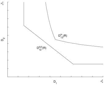
Figure 4: Comparison of $\mathcal{D}^{in}_{12}(R)$ and $\mathcal{D}^{out}_{12}(R)$

V-D An Extreme Case

Theorem 6

Let $\mathcal{Q}_{e}=\{(R_{1},D_{1},D_{2},D_{3}):(R_{1},\infty,D_{1},D_{2},D_{3})\in\mathcal{Q}\}$. We have $(R_{1},D_{1},D_{2},D_{3})\in\mathcal{Q}_{e}$ if and only if $D_{2}\geq D_{2,\min}$ and

$$R_{1}\geq\left\{\begin{array}[]{lc}\frac{1}{2}\log\frac{\sigma_{X}^{4}\sigma_{N_{2}}^{4}}{\left(\sigma_{N_{2}}^{2}+D_{1}\right)\left(D_{3}\sigma_{X}^{2}\sigma_{N_{1}}^{2}+D_{3}\sigma_{X}^{2}\sigma_{N_{2}}^{2}+D_{3}\sigma_{N_{1}}^{2}\sigma_{N_{2}}^{2}-\sigma_{X}^{2}\sigma_{N_{1}}^{2}\sigma_{N_{2}}^{2}\right)},&D_{3}\leq\frac{D_{1}\sigma^{2}_{N_{2}}}{D_{1}+\sigma^{2}_{N_{2}}}\\ R(D_{1},\sigma^{2}_{N_{1}}),&D_{3}>\frac{D_{1}\sigma^{2}_{N_{2}}}{D_{1}+\sigma^{2}_{N_{2}}}.\end{array}\right.$$

Proof:

Since $R_{2}=\infty$, we can assume that $\{Y_{2}(t)\}_{t=1}^{\infty}$ is directly present at decoder 2 and decoder 3. Hence any $D_{2}\geq D_{2,\min}$ is achievable. Now only $(R_{1},D_{1},D_{3})$ remain to be characterized. The achievability part follows directly by evaluating $\mathcal{Q}_{in}$ with $\sigma^{2}_{T_{21}}=\sigma^{2}_{T_{22}}=0$. For the converse, it is clear that $R_{1}\geq R(D_{1},\sigma^{2}_{N_{1}})$, which resolves the case $D_{3}>{D_{1}\sigma^{2}_{N_{2}}}/{(D_{1}+\sigma^{2}_{N_{2}})}$. For the case $D_{3}\leq{D_{1}\sigma^{2}_{N_{2}}}/{(D_{1}+\sigma^{2}_{N_{2}})}$, the details are left to Appendix IV. ∎

Remark: The converse can not be reduced from $\mathcal{Q}_{out}$, which shows that our outer bound in not tight.

Theorem 6 implies that

$$D^{*}_{3}(R_{1},\infty)=\frac{\sigma_{X}^{4}\sigma_{N_{2}}^{4}\exp\left(-2R_{1}\right)+\sigma_{X}^{2}\sigma_{N_{1}}^{2}\sigma_{N_{2}}^{2}\left(\sigma_{X}^{2}+\sigma_{N_{2}}^{2}\right)}{\left(\sigma_{X}^{2}+\sigma_{N_{2}}^{2}\right)\left(\sigma_{X}^{2}\sigma_{N_{1}}^{2}+\sigma_{X}^{2}\sigma_{N_{2}}^{2}+\sigma_{N_{1}}^{2}\sigma_{N_{2}}^{2}\right)},$$

and $\min\{D_{1}:(R_{1},\infty,D_{1},D_{2},D^{*}_{3}(R_{1},\infty))\in\mathcal{Q}\}=\sigma^{2}_{X}$ for $D_{2}\geq D_{2,\min}$. That is to say, for this extreme case, if decoder 3 achieves the minimum $D_{3}$ for a given $R_{1}$, then it is impossible for decoder 1 to make a nontrivial estimation of $\{X(t)\}_{t=1}^{\infty}$.

V-E Noisy Multiple Description for the Gaussian Case

Now consider the case when both encoder 1 and encoder 2 can observe $\{Y_{1}(t)\}_{t=1}^{\infty}$ and $\{Y_{2}(t)\}_{t=1}^{\infty}$ simultaneously. Clearly, the rate distortion region of this problem (which we denote by $\mathcal{Q}^{\prime}$) is an outer bound of $\mathcal{Q}$.

If we assume encoder 1 and encoder 2 can only observe $\{\mathbb{E}(X(t)|Y_{1}(t),Y_{2}(t))\}_{t=1}^{\infty}$, and let $\mathcal{Q}^{\prime\prime}$ be the rate distortion region for this case, then clearly we have $\mathcal{Q}^{\prime\prime}\subseteq\mathcal{Q}^{\prime}$ since $\{\mathbb{E}(X(t)|Y_{1}(t),Y_{2}(t))\}_{t=1}^{\infty}$ can be computed from $\{Y_{1}(t)\}_{t=1}^{\infty}$ and $\{Y_{2}(t)\}_{t=1}^{\infty}$.

Theorem 7

$\mathcal{Q}^{\prime}=\mathcal{Q}^{\prime\prime}=\mathcal{T}$, where

$$\mathcal{T}=\left\{(R_{1},R_{2},D_{1},D_{2},D_{3}):R_{1}+R_{2}\geq\frac{1}{2}\log\frac{d_{X}}{d_{3}}+\gamma(d_{1},d_{2},d_{3}),R_{i}\geq\frac{1}{2}\log\frac{d_{X}}{d_{i}},i=1,2\right\},$$

and

$$\gamma(d_{1},d_{2},d_{3})=\left\{\begin{array}[]{ll}0,\hskip 202.35622ptd_{3}\leq d_{1}+d_{2}-d_{X}\\ \frac{1}{2}\log\frac{d_{X}d_{3}}{d_{1}d_{2}},\hskip 159.71718ptd_{3}\geq\left(\frac{1}{d_{1}}+\frac{1}{d_{2}}-\frac{1}{d_{X}}\right)^{-1}\\ \frac{1}{2}\log\frac{(d_{X}-d_{3})^{2}}{(d_{X}-d_{3})^{2}-[\sqrt{(d_{X}-d_{1})(d_{X}-d_{2})}-\sqrt{(d_{1}-d_{3})(d_{2}-d_{3})}]^{2}},\mbox{\quad otherwise}.\end{array}\right.$$

Proof:

As defined before, let $S(t)=\mathbb{E}(X(t)|Y_{1}(t),Y_{2}(t))$ and $\theta(t)=X(t)-S(t)$, $t=1,2,\cdots$. We have $\mathbb{E}\theta^{2}(t)=D_{3,\min}$ and $\mathbb{E}S^{2}(t)=\sigma^{2}_{X}-D_{3,\min}=d_{X}$.

Now we view $\{S(t)\}_{t=1}^{\infty}$ as the source, and let $\mathcal{Q}_{S}$ be the multiple description rate-distortion region for $\{S(t)\}_{t=1}^{\infty}$. It was proved by Ozarow [20] that $(R_{1},R_{2},D_{1},D_{2},D_{3})\in\mathcal{Q}_{S}$ if and only if

$$R_{i} \geq \frac{1}{2}\log\frac{d_{X}}{D_{i}},\quad i=1,2,$$

$$R_{3} \geq \frac{1}{2}\log\frac{d_{X}}{D_{3}}+\gamma_{S}(D_{1},D_{2},D_{3}),$$

where

$$\gamma_{S}(D_{1},D_{2},D_{3})=\left\{\begin{array}[]{ll}0,\hskip 202.35622ptD_{3}\leq D_{1}+D_{2}-d_{X}\\ \frac{1}{2}\log\frac{d_{X}D_{3}}{D_{1}D_{2}},\hskip 159.71718ptD_{3}\geq\left(\frac{1}{D_{1}}+\frac{1}{D_{2}}-\frac{1}{d_{X}}\right)^{-1}\\ \frac{1}{2}\log\frac{(d_{X}-D_{3})^{2}}{(d_{X}-D_{3})^{2}-[\sqrt{(d_{X}-D_{1})(d_{X}-D_{2})}-\sqrt{(D_{1}-D_{3})(D_{2}-D_{3})}]^{2}},\mbox{\quad otherwise}.\end{array}\right.$$

Since $\{\theta(t)\}_{t=1}^{n}$ is independent of $\{Y_{1}(t),Y_{2}(t)\}_{t=1}^{n}$ and thus is independent of $\{\hat{X}_{1}(t),\hat{X}_{2}(t),\hat{X}_{3}(t)\}_{t=1}^{n}$, we have

$$\frac{1}{n}\mathbb{E}\sum\limits_{t=1}^{n}(X(t)-\hat{X}_{i}(t))^{2} = \frac{1}{n}\sum\limits_{t=1}^{n}\mathbb{E}(S(t)+\theta(t)-\hat{X}_{i}(t))^{2}$$

$$= \frac{1}{n}\sum\limits_{t=1}^{n}\left[\mathbb{E}\theta^{2}(t)+\mathbb{E}(S(t)-\hat{X}_{i}(t))^{2}\right]$$

$$= D_{3,\min}+\frac{1}{n}\sum\limits_{t=1}^{n}\mathbb{E}(S(t)-\hat{X}_{i}(t))^{2},\quad i=1,2,3.$$

Hence $(R_{1},R_{2},D_{1},D_{2},D_{3})\in\mathcal{Q}^{\prime}$(or $\mathcal{Q}^{\prime\prime}$) if and only if $(R_{1},R_{2},D_{1}-D_{3,\min},D_{2}-D_{3,\min},D_{3}-D_{3,\min})\in\mathcal{Q}_{S}$ (i.e., $(R_{1},R_{2},d_{1},d_{2},d_{3})\in\mathcal{Q}_{S}$). The proof is complete. ∎

Remark: Theorem 7 is still true when $N_{1}(t)$ and $N_{2}(t)$ are correlated (with correlation coefficient $\rho_{N}$), now

$$D_{3,\min}=\left(\frac{1}{\sigma^{2}_{X}}+\frac{\sigma^{2}_{N_{1}}+\sigma^{2}_{N_{2}}-2\rho_{N}\sigma_{N_{1}}\sigma_{N_{2}}}{(1-\rho_{N}^{2})\sigma^{2}_{N_{1}}\sigma^{2}_{N_{2}}}\right)^{-1}.$$

Note: $D_{3,\min}=(1/\sigma^{2}_{X}+1/\sigma^{2}_{N})^{-1}$ if $\sigma^{2}_{N_{1}}=\sigma^{2}_{N_{2}}=\sigma^{2}_{N}$ and $\rho_{N}=1$.

VI Conclusion

We proposed a robust distributed source coding scheme which flexibly trades off between system robustness and compression efficiency. The achievable rate distortion region of this scheme was analyzed in detail for the Gaussian case. But a complete characterization of the rate distortion region $\mathcal{Q}$, even for the Gaussian case, remains open. We believe that the following problem deserves special attention. For the Gaussian case, $\mathcal{Q}|_{\sigma^{2}_{N_{1}}=\sigma^{2}_{N_{2}}=0}$ is the rate distortion region of the multiple description problem, which has been completely characterized in [20]. The question is whether $\mathcal{Q}$ converges to $\mathcal{Q}|_{\sigma^{2}_{N_{1}}=\sigma^{2}_{N_{2}}=0}$ as $\sigma^{2}_{N_{1}}$ and $\sigma^{2}_{N_{2}}$ go to zero. A solution to this problem will have many interesting implications and can significantly deepen our understanding of the multiple description problem and the distributed source coding problem.

Appendix A Proof of Theorem 1

The proof of Theorem 1 employs techniques which have already been established in the literature, especially in [43][47][53][54]. Hence we only give a sketch here.

For each $U_{1},U_{2},W_{1}$ and $W_{2}$ satisfying Property (i) and (iii), we prove the admissibility of the rate tuple $(R_{1},R_{2})$, where

$$R_{1} = I(Y_{1};U_{1})+I(Y_{1};W_{1}|U_{1},U_{2},W_{2}),$$

$$R_{2} = I(Y_{2};U_{2})+I(Y_{2};W_{2}|U_{1},U_{2}).$$

Then by symmetry, the rate tuple $(R^{\prime}_{1},R^{\prime}_{2})$ with

$$R^{\prime}_{1} = I(Y_{1};U_{1})+I(Y_{1};W_{1}|U_{1},U_{2}),$$

$$R^{\prime}_{2} = I(Y_{2};U_{2})+I(Y_{2};W_{2}|U_{1},U_{2},W_{1})$$

is also admissible. It’s easy to check that

$$I(Y_{1};W_{1}|U_{1},U_{2},W_{2})+I(Y_{2};W_{2}|U_{1},U_{2})$$

$$= I(Y_{1};W_{1}|U_{1},U_{2})+I(Y_{2};W_{2}|U_{1},U_{2},W_{1})$$

$$= I(Y_{1},Y_{2};W_{1},W_{2}|U_{1},U_{2}),$$

now Theorem 1 follows by timesharing $(R_{1},R_{2})$ and $(R^{\prime}_{1},R^{\prime}_{2})$.

It was established in [47] that for any positive $\epsilon$ and sufficiently large $n$ with

$$|\mathcal{C}^{(n)}_{1}|\leq\exp(n(I(Y_{1};U_{1})+I(Y_{1};W_{1}|U_{1},U_{2},W_{2})+\epsilon)),$$

decoder 1 and decoder 3 can recover $u^{n}_{1}$ and construct $\hat{x}^{n}_{1}$ with $\hat{x}_{1}(t)=f_{1}(u_{1}(t)),t=1,2,\cdots,n,$ such that

$$\frac{1}{n}E\sum\limits_{t=1}^{n}d(X(t),\hat{X}_{1}(t))<D_{1}+\epsilon,$$

and provided $u_{2}^{n}$ and $w_{2}^{n}$ are available to decoder 3, it can further recover $w_{1}^{n}$ and use $w^{n}_{1},w^{n}_{2},u^{n}_{1},u^{n}_{2}$ to construct $\hat{x}^{n}_{3}$ with $\hat{x}_{3}(t)=f_{3}\left(w_{1}(t),w_{2}(t),u_{1}(t),u_{2}(t)\right),t=1,2,\cdots,n,$ such that the average distortion is less than or equal to $D_{3}+\epsilon$.

Again by [47], with

$$|\mathcal{C}^{(n)}_{2}|\leq\exp(n(I(Y_{2};W_{2})+I(Y_{2};U_{2}|W_{1},W_{2})+\epsilon)),$$

decoder 2 and decoder 3 can recover $u^{n}_{2}$ and construct $\hat{x}^{n}_{2}$ with $\hat{x}_{2}(t)=f_{2}(u_{2}(t)),t=1,2,\cdots,n,$ such that

$$\frac{1}{n}E\sum\limits_{t=1}^{n}d(X(t),\hat{X}_{2}(t))<D_{2}+\epsilon,$$

and provided $u_{1}^{n}$ are available to decoder 3, it can further recover $w_{2}^{n}$.

In summary, decoder $i$ recovers $u^{n}_{i}$ $(i=1,2)$, and decoder 3 recovers $u^{n}_{1},u^{n}_{2},w^{n}_{1},w^{n}_{2}$ with the decoding order $(u^{n}_{1},u^{n}_{2})\rightarrow w^{n}_{2}\rightarrow w^{n}_{1}$.

Thus we have established the admissibility of the rate tuple $(R_{1},R_{2})$ and completed the proof.

Appendix B Derivation of the Outer bound

Let $r_{i1}=I(X^{n};f^{(n)}_{E,i}(Y^{n}_{i}))/n,r_{i2}=I(Y_{i}^{n};f^{(n)}_{E,i}(Y^{n}_{i})|X^{n})/n$, $i=1,2$. The following lemmas were proved in [17] with the method developed by Oohama [14].

Lemma 2

$$\frac{1}{\sigma_{X}^{2}}\exp\left(2r_{i1}\right) \leq \frac{1}{\sigma_{X}^{2}}+\frac{1-\exp\left(2r_{i2}\right)}{\sigma_{N_{i}}^{2}}\quad i=1,2,$$

$$\frac{1}{\sigma_{X}^{2}}\exp\left(\frac{2}{n}I\left(X^{n};f^{(n)}_{E,1}(Y^{n}_{1})f^{(n)}_{E,2}(Y^{n}_{2})\right)\right) \leq \frac{1}{\sigma_{X}^{2}}+\frac{1-\exp\left(-2r_{12}\right)}{\sigma_{N_{i}}^{2}}+\frac{1-\exp(-2r_{22})}{\sigma_{N_{2}}^{2}}.$$

Now we are ready to derive the outer bound.

Proof:

By data processing inequality, we have

$$I\left(X^{n};f^{(n)}_{E,i}(Y^{n}_{i})\right)\geq I\left(X^{n};\hat{X}^{n}_{i}\right)\geq\frac{n}{2}\log\frac{\sigma_{X}^{2}}{D_{i}},\quad i=1,2$$ (27)

$$I\left(X^{n};f^{(n)}_{E,1}(Y^{n}_{1})f^{(n)}_{E,2}(Y^{n}_{2})\right)\geq I\left(X^{n};\hat{X}^{n}_{3}\right)\geq\frac{n}{2}\log\frac{\sigma_{X}^{2}}{D_{3}}.$$ (28)

It follows from (27), (28) and Lemma 2 that

$$\frac{1}{D_{i}} \leq \frac{\exp(2r_{i1})}{\sigma^{2}_{X}},\quad i=1,2,$$

$$\frac{1}{D_{3}} \leq \frac{1}{\sigma^{2}_{X}}+\frac{1-\exp(-2r_{12})}{\sigma^{2}_{N_{1}}}+\frac{1-\exp(-2r_{12})}{\sigma^{2}_{N_{1}}}.$$

Since $X^{n}\rightarrow Y^{n}_{i}\rightarrow f^{(n)}_{E,i}(Y^{n}_{i})$, $i=1,2$, we have

$$R_{i} \geq \frac{1}{n}I\left(Y^{n}_{i};f^{(n)}_{E,i}(Y^{n}_{i})\right)\geq\frac{1}{n}I\left(X^{n},Y^{n}_{i};f^{(n)}_{E,i}(Y^{n}_{i})\right)$$

$$= \frac{1}{n}I\left(X^{n};f^{(n)}_{E,i}(Y^{n}_{i})\right)+\frac{1}{n}I\left(\left.Y_{i}^{n};f^{(n)}_{E,i}(Y^{n}_{i})\right|X^{n}\right)$$

$$= r_{i1}+r_{i2}\quad i=1,2.$$

Now we proceed to derive a lower bound on $r_{11}+r_{21}$,

$$n(r_{11}+r_{21})$$ (29)

$$= I\left(X^{n};f^{(n)}_{E,1}(Y^{n}_{1})\right)+I\left(X^{n};f^{(n)}_{E,2}(Y^{n}_{2})\right)$$

$$\stackrel{{\scriptstyle(a)}}{{=}} I\left(X^{n};f^{(n)}_{E,1}(Y^{n}_{1}),f^{(n)}_{E,2}(Y^{n}_{2})\right)+I\left(f^{(n)}_{E,1}(Y^{n}_{1});f^{(n)}_{E,2}(Y^{n}_{2})\right)-I\left(\left.f^{(n)}_{E,1}(Y^{n}_{1});f^{(n)}_{E,2}(Y^{n}_{2})\right|X^{n}\right)$$

$$\stackrel{{\scriptstyle(b)}}{{=}} I\left(X^{n};f^{(n)}_{E,1}(Y^{n}_{1}),f^{(n)}_{E,2}(Y^{n}_{2})\right)+I\left(f^{(n)}_{E,1}(Y^{n}_{1});f^{(n)}_{E,2}(Y^{n}_{2})\right)$$

where (a) follows from the identity

$$I\left(A;BC\right)=I\left(A;B\right)+I\left(A;C\right)+I\left(B;C|A\right)-I\left(B;C\right).$$ (30)

and (b) is because $f^{(n)}_{E,1}(Y^{n}_{1})\rightarrow X^{n}\rightarrow f^{(n)}_{E,2}(Y^{n}_{2})$. Now applying data processing inequality, we have

$$n\left(r_{11}+r_{21}\right) \geq I\left(X^{n};\hat{X}^{n}_{3}\right)+I\left(f^{(n)}_{E,1}(Y^{n}_{1});f^{(n)}_{E,2}(Y^{n}_{2})\right)$$ (31)

$$\geq\frac{1}{2}\log\frac{\sigma^{2}_{X}}{D_{3}}+I\left(f^{(n)}_{E,1}(Y^{n}_{1});f^{(n)}_{E,2}(Y^{n}_{2})\right).$$

To lower-bound $I\left(f^{(n)}_{E,1}(Y^{n}_{1});f^{(n)}_{E,2}(Y^{n}_{2})\right)$, we introduce an auxiliary random vector $Z^{n}$ such that $Z(t)=S(t)+M(t),t=1,2,\cdots,n$, where the $M(t)^{\prime}s$ are i.i.d zero-mean Gaussian random variables with variance $\sigma^{2}_{M}$ (which will be optimized later). We assume that $M^{n}$ is independent of $(X^{n},Y^{n}_{1},Y^{n}_{2})$. Since $\theta^{n}$ is indepedent of $Y^{n}_{1},Y^{n}_{2}$ and thus independent of $\hat{X}^{n}_{1},\hat{X}^{n}_{2}$, we have

$$D_{i} \geq \frac{1}{n}\sum\limits_{t=1}^{n}{\mathbb{E}\left(X(t)-\hat{X}_{i}(t)\right)^{2}}$$

$$= \frac{1}{n}\sum\limits_{t=1}^{n}{\mathbb{E}(S(t)+\theta(t)-\hat{X}_{i}(t))^{2}}$$

$$= \frac{1}{n}\sum\limits_{t=1}^{n}{\mathbb{E}\left(S(t)-\hat{X}_{i}(t)\right)^{2}}+D_{3,\min},$$

i.e.,

$$\frac{1}{n}\sum{\mathbb{E}\left(S(t)-\hat{X}_{i}(t)\right)^{2}}\leq D_{i}-D_{3,\min}=d_{i},\quad i=1,2.$$

Since

$$\frac{1}{n}\sum{\mathbb{E}\left(Z(t)-\hat{X}_{i}(t)\right)^{2}} = \frac{1}{n}\sum{\mathbb{E}\left(S(t)-\hat{X}_{i}(t)\right)^{2}}+\frac{1}{n}\sum{\mathbb{E}M^{2}(t)}$$

$$\leq d_{i}+\sigma^{2}_{M},\quad i=1,2,$$

by rate distortion theory,

$$I\left(Z^{n};\hat{X}^{n}_{i}\right)\geq\frac{n}{2}\log\left(\frac{d_{X}+\sigma^{2}_{M}}{d_{i}+\sigma^{2}_{M}}\right),\quad i=1,2.$$

Now applying the identity (30) to $I\left(f^{(n)}_{E,1}(Y^{n}_{1});f^{(n)}_{E,2}(Y^{n}_{2})\right)$, we get

$$I\left(f^{(n)}_{E,1}(Y^{n}_{1});f^{(n)}_{E,2}(Y^{n}_{2})\right)$$ (32)

$$= I\left(Z^{n};f^{(n)}_{E,1}(Y^{n}_{1})\right)+I\left(Z^{n};f^{(n)}_{E,2}(Y^{n}_{2})\right)+I\left(\left.f^{(n)}_{E,1}(Y^{n}_{1});f^{(n)}_{E,2}(Y^{n}_{2})\right|Z^{n}\right)-I\left(Z^{n};f^{(n)}_{E,1}(Y^{n}_{1}),f^{(n)}_{E,2}(Y^{n}_{2})\right)$$

$$\geq I\left(Z^{n};\hat{X}^{n}_{1}\right)+I\left(Z^{n};\hat{X}^{n}_{2}\right)-I\left(Z^{n};f^{(n)}_{E,1}(Y^{n}_{1}),f^{(n)}_{E,2}(Y^{n}_{2})\right)$$

$$\geq \frac{n}{2}\log\left[\left(\frac{d_{X}+\sigma^{2}_{M}}{d_{1}+\sigma^{2}_{M}}\right)\left(\frac{d_{X}+\sigma^{2}_{M}}{d_{2}+\sigma^{2}_{M}}\right)\right]-I\left(Z^{n};f^{(n)}_{E,1}(Y^{n}_{1}),f^{(n)}_{E,2}(Y^{n}_{2})\right).$$

We upper-bound $I\left(Z^{n};f^{(n)}_{E,1}(Y^{n}_{1}),f^{(n)}_{E,2}(Y^{n}_{2})\right)$ as follows:

$$I\left(Z^{n};f^{(n)}_{E,1}(Y^{n}_{1}),f^{(n)}_{E,2}(Y^{n}_{2})\right)$$ (33)

$$= h(Z^{n})-h\left(Z^{n}\left|f^{(n)}_{E,1}(Y^{n}_{1}),f^{(n)}_{E,2}(Y^{n}_{2})\right.\right)$$

$$= \frac{n}{2}\log\left[2\pi e\left(d_{X}+\sigma^{2}_{M}\right)\right]-h\left(S^{n}+M^{n}|f^{(n)}_{E,1}(Y^{n}_{1}),f^{(n)}_{E,2}(Y^{n}_{2})\right)$$

$$\stackrel{{\scriptstyle(c)}}{{\leq}} \frac{n}{2}\log\left[2\pi e\left(d_{X}+\sigma^{2}_{M}\right)\right]-\frac{n}{2}\log\left\{\exp\left[\frac{2}{n}h(S^{n}|f^{(n)}_{E,1}(Y^{n}_{1}),f^{(n)}_{E,2}(Y^{n}_{2}))\right]+2\pi e\sigma^{2}_{M}\right\},$$

where (c) follows from the conditional version of entropy power inequality [55]. Since

$$h\left(S^{n}\left|f^{(n)}_{E,1}(Y^{n}_{1}),f^{(n)}_{E,2}(Y^{n}_{2})\right.\right)$$

$$= h\left(S^{n}\left|X^{n},f^{(n)}_{E,1}(Y^{n}_{1}),f^{(n)}_{E,2}(Y^{n}_{2})\right.\right)+I\left(X^{n};\hat{X}^{n}\left|f^{(n)}_{E,1}(Y^{n}_{1}),f^{(n)}_{E,2}(Y^{n}_{2})\right.\right)$$

$$= h\left(S^{n}\left|X^{n},f^{(n)}_{E,1}(Y^{n}_{1}),f^{(n)}_{E,2}(Y^{n}_{2})\right.\right)+I\left(X^{n};S^{n},f^{(n)}_{E,1}(Y^{n}_{1}),f^{(n)}_{E,2}(Y^{n}_{2})\right)-I\left(X^{n};f^{(n)}_{E,1}(Y^{n}_{1}),f^{(n)}_{E,2}(Y^{n}_{2})\right)$$

$$= h\left(S^{n}\left|X^{n},f^{(n)}_{E,1}(Y^{n}_{1}),f^{(n)}_{E,2}(Y^{n}_{2})\right.\right)+I\left(X^{n};S^{n}\right)-I\left(X^{n};f^{(n)}_{E,1}(Y^{n}_{1}),f^{(n)}_{E,2}(Y^{n}_{2})\right),$$

where the last equality follows from $X^{n}\rightarrow S^{n}\rightarrow\left(f^{(n)}_{E,1}(Y^{n}_{1}),f^{(n)}_{E,2}(Y^{n}_{2})\right)$, we have

$$\exp\left(\frac{2}{n}h\left(S^{n}\left|f^{(n)}_{E,1}(Y^{n}_{1}),f^{(n)}_{E,2}(Y^{n}_{2})\right.\right)\right)$$ (34)

$$= \exp\left(h\left(S^{n}\left|X^{n},f^{(n)}_{E,1}(Y^{n}_{1}),f^{(n)}_{E,2}(Y^{n}_{2})\right.\right)\right)\exp\left(I\left(X^{n};S^{n}\right)\right)\exp\left(-I\left(X^{n};f^{(n)}_{E,1}(Y^{n}_{1}),f^{(n)}_{E,2}(Y^{n}_{2})\right)\right)$$

$$= \frac{\sigma^{2}_{X}}{D_{3,\min}}\exp\left(h(S^{n}|X^{n},f^{(n)}_{E,1}(Y^{n}_{1}),f^{(n)}_{E,2}(Y^{n}_{2}))\right)\exp\left(-I(X^{n};f^{(n)}_{E,1}(Y^{n}_{1}),f^{(n)}_{E,2}(Y^{n}_{2}))\right).$$

Now we shall derive a lower bound on $\exp\left(\frac{2}{n}h\left(S^{n}\left|X^{n},f^{(n)}_{E,1}(Y^{n}_{1}),f^{(n)}_{E,2}(Y^{n}_{2})\right.\right)\right)$. Since conditioned on $\left(X^{n},f^{(n)}_{E,1}(Y^{n}_{1}),f^{(n)}_{E,2}(Y^{n}_{2})\right)$, $Y^{n}_{1}$ and $Y^{n}_{2}$ are independent, by the conditional version of entropy power inequality [55], we have

$$\exp\left(\frac{2}{n}h\left(S^{n}\left|X^{n},f^{(n)}_{E,1}(Y^{n}_{1}),f^{(n)}_{E,2}(Y^{n}_{2})\right.\right)\right)$$ (35)

$$\geq \sum\limits_{i=1}^{2}\exp\left(\frac{2}{n}h\left(\left.\frac{D_{3,\min}}{\sigma^{2}_{N_{i}}}Y^{n}_{i}\right|X^{n},f^{(n)}_{E,1}(Y^{n}_{1}),f^{(n)}_{E,2}(Y^{n}_{2})\right)\right)$$

$$= D^{2}_{3,\min}\sum\limits_{i=1}^{2}\frac{1}{\sigma^{4}_{N_{i}}}\exp\left(\frac{2}{n}h\left(Y^{n}_{i}\left|X^{n},f^{(n)}_{E,1}(Y^{n}_{1}),f^{(n)}_{E,2}(Y^{n}_{2})\right.\right)\right)$$

$$= D^{2}_{3,\min}\sum\limits_{i=1}^{2}\frac{1}{\sigma^{4}_{N_{i}}}\exp\left(\frac{2}{n}h(Y^{n}_{i}|X^{n})-\frac{2}{n}I\left(\left.Y^{n}_{i};f^{(n)}_{E,i}(Y^{n}_{i})\right|X^{n}\right)\right)$$

$$= 2\pi eD^{2}_{3,\min}\sum\limits_{i=1}^{2}\frac{\exp\left(-2r_{2i}\right)}{\sigma^{2}_{N_{i}}}.$$

Thus by (34) and (35),

$$\exp\left(\frac{2}{n}h\left(S^{n}\left|f^{(n)}_{E,1}(Y^{n}_{1}),f^{(n)}_{E,2}(Y^{n}_{2})\right.\right)\right)$$ (36)

$$\geq 2\pi e\sigma^{2}_{X}D_{3,\min}\left(\sum\limits_{i=1}^{2}\frac{\exp\left(-2r_{2i}\right)}{\sigma^{2}_{N_{i}}}\right)\exp\left(-\frac{2}{n}I\left(X^{n};f^{(n)}_{E,1}(Y^{n}_{1}),f^{(n)}_{E,2}(Y^{n}_{2})\right)\right).$$

Combining (33) and (36) yields that

$$I\left(Z^{n};f^{(n)}_{E,1}(Y^{n}_{1}),f^{(n)}_{E,2}(Y^{n}_{2})\right)\leq\frac{n}{2}\log(d_{X}+\sigma^{2}_{M}))$$

$$- \frac{n}{2}\log\left(\sigma^{2}_{X}D_{3,\min}\left(\sum\limits_{i=1}^{2}\frac{\exp\left(-2r_{2i}\right)}{\sigma^{2}_{N_{i}}}\right)\exp\left(-\frac{2}{n}I\left(X^{n};f^{(n)}_{E,1}(Y^{n}_{1}),f^{(n)}_{E,2}(Y^{n}_{2})\right)\right)+\sigma^{2}_{M}\right).$$

Substitute (B) into (32) and then apply (29),

$$I\left(f^{(n)}_{E,1}(Y^{n}_{1});f^{(n)}_{E,2}(Y^{n}_{2})\right)$$

$$\geq \frac{n}{2}\log\left(\frac{d_{X}+\sigma^{2}_{M}}{(d_{1}+\sigma^{2}_{M})(d_{2}+\sigma^{2}_{M})}\right)$$

$$+\frac{n}{2}\log\left(\sigma^{2}_{X}D_{3,\min}\left(\sum\limits_{i=1}^{2}\frac{\exp\left(-2r_{2i}\right)}{\sigma^{2}_{N_{i}}}\right)\exp\left(-\frac{2}{n}I\left(X^{n};f^{(n)}_{E,1}(Y^{n}_{1}),f^{(n)}_{E,2}(Y^{n}_{2})\right)\right)+\sigma^{2}_{M}\right)$$

$$\geq \frac{n}{2}\log\left(\frac{d_{X}+\sigma^{2}_{M}}{(d_{1}+\sigma^{2}_{M})(d_{2}+\sigma^{2}_{M})}\right)$$

$$+\frac{n}{2}\log\left(\sigma^{2}_{X}D_{3,\min}\left(\sum\limits_{i=1}^{2}\frac{\exp\left(-2r_{2i}\right)}{\sigma^{2}_{N_{i}}}\right)\exp\left(\frac{2}{n}I\left(f^{(n)}_{E,1}(Y^{n}_{1});f^{(n)}_{E,2}(Y^{n}_{2})\right)\right)\exp\left(-2(r_{11}+r_{21})\right)+\sigma^{2}_{M}\right),$$

which can be rewritten as

$$\exp\left(\frac{2}{n}I\left(f^{(n)}_{E,1}(Y^{n}_{1});f^{(n)}_{E,2}(Y^{n}_{2})\right)\right)$$ (37)

$$\geq \frac{\left(d_{X}+\sigma^{2}_{M}\right)\sigma^{2}_{M}}{\left(d_{1}+\sigma^{2}_{M}\right)\left(d_{2}+\sigma^{2}_{M}\right)-\sigma^{2}_{X}D_{3,\min}\left(d_{X}+\sigma^{2}_{M}\right)\exp\left(-2\left(r_{11}+r_{21}\right)\right)\left(\sum\limits_{i=1}^{2}\frac{\exp\left(-2r_{2i}\right)}{\sigma^{2}_{N_{i}}}\right)}.$$

Combining (31) and (37) yields that

$$\exp\left(2\left(r_{11}+r_{21}\right)\right)$$

$$\geq \frac{\sigma^{2}_{X}\sigma^{2}_{M}\left(\sigma^{2}_{X}+\sigma^{2}_{M}\right)}{D_{3}\left(\left(d_{1}+\sigma^{2}_{M}\right)\left(d_{2}+\sigma^{2}_{M}\right)-\sigma^{2}_{X}D_{3,\min}\left(d_{X}+\sigma^{2}_{M}\right)\exp\left(-2\left(r_{11}+r_{21}\right)\right)\left(\sum\limits_{i=1}^{2}\frac{\exp\left(-2r_{2i}\right)}{\sigma^{2}_{N_{i}}}\right)\right)},$$

which can be further written as

$$r_{11}+r_{21}\geq\frac{1}{2}\log\frac{\sigma^{2}_{X}}{D_{3}}+\eta(\sigma^{2}_{M},d_{1},d_{2},\zeta),$$

where

$$\zeta=D_{3,\min}D_{3}\left(\sum\limits_{i=1}^{2}\frac{\exp\left(-2r_{2i}\right)}{\sigma^{2}_{N_{i}}}\right),$$

$$\eta(\sigma^{2}_{M},d_{1},d_{2},\zeta)=\frac{1}{2}\log\frac{\left(d_{X}+\sigma^{2}_{M}\right)\left(\zeta+\sigma^{2}_{M}\right)}{\left(d_{1}+\sigma^{2}_{M}\right)\left(d_{2}+\sigma^{2}_{M}\right)}.$$

Calculus shows that

$$\sup\limits_{\sigma^{2}_{M}}\eta(\sigma^{2}_{M},d_{1},d_{2},\zeta)$$

$$=\left\{\begin{array}[]{ll}\eta(\infty,d_{1},d_{2},\zeta)=0,\hskip 187.90244pt\zeta\leq d_{1}+d_{2}-d_{X}\\ \eta(0,d_{1},d_{2},\zeta)=\frac{1}{2}\log\frac{d_{X}\zeta}{d_{1}d_{2}},\hskip 153.93544pt\zeta\geq\left(\frac{1}{d_{1}}+\frac{1}{d_{2}}-\frac{1}{d_{X}}\right)^{-1}\\ \eta(\hat{\sigma}^{2}_{M},d_{1},d_{2},\zeta)=\frac{1}{2}\log\frac{(d_{X}-\zeta)^{2}}{(d_{X}-\zeta)^{2}-[\sqrt{(d_{X}-d_{1})(d_{X}-d_{2})}-\sqrt{(d_{1}-\zeta)(d_{2}-\zeta)}]^{2}},\mbox{ otherwise}\\ \end{array}\right.$$

where

$$\hat{\sigma}^{2}_{M}=\frac{d_{1}d_{2}-d_{X}\zeta+\sqrt{(d_{X}-d_{1})(d_{X}-d_{2})(d_{1}-\zeta)(d_{2}-\zeta)}}{d_{X}+\zeta-d_{1}-d_{2}}.$$

∎

Appendix C Proof of Lemma 1

Define the functions $y_{1}=\phi_{1}(x_{1})$ and $y_{2}=\phi_{2}(x_{2})$ via the following parametric forms:

$$x_{1} = \frac{1}{2}\log\left(\frac{1}{\sigma^{2}_{X}}+\frac{1-\exp(-2\alpha_{1})}{\sigma^{2}_{N}}\right)+\frac{1}{2}\log\sigma^{2}_{X}+\alpha_{1},$$

$$y_{1} = \frac{1}{2}\log\left(\frac{1}{\sigma^{2}_{X}}+\frac{2-2\exp(-2\alpha_{1})}{\sigma^{2}_{N}}\right)-\frac{1}{2}\log\left(\frac{1}{\sigma^{2}_{X}}+\frac{1-\exp(-2\alpha_{1})}{\sigma^{2}_{N}}\right)+\alpha_{1},$$

and

$$x_{2} = \frac{1}{2}\log\left(\frac{1}{\sigma^{2}_{X}}+\frac{2-2\exp(-2\alpha_{2})}{\sigma^{2}_{N}}\right)-\frac{1}{2}\log\left(\frac{1}{\sigma^{2}_{X}}+\frac{1-\exp(-2\alpha_{2})}{\sigma^{2}_{N}}\right)+\theta_{2},$$

$$y_{2} = \frac{1}{2}\log\left(\frac{1}{\sigma^{2}_{X}}+\frac{1-\exp(-2\alpha_{2})}{\sigma^{2}_{N}}\right)+\frac{1}{2}\log\sigma^{2}_{X}+\alpha_{2},$$

where $\alpha_{1},\alpha_{2}\geq 0$. Define $\Omega=\{(R_{1},R_{2})\in\mathcal{R}^{2}_{+}:\phi_{1}(R_{1})\leq R_{2}\leq\phi_{2}(R_{1})\}$. It is easy to check that $(R,R)$ is an interior point of $\Omega$ for any $R>0$.

Let $\Gamma$ denote the line segment from $(R^{\prime}_{1},R^{\prime}_{2})$ to $(R^{\prime\prime}_{1},R^{\prime\prime}_{2})$. It is clear that $D^{*}_{3}(R_{1},R_{2})$ must be a convex function of $(R_{1},R_{2})$. Hence we have $\lambda_{1}D^{*}_{3}(R^{\prime}_{1},R^{\prime}_{2})+\lambda_{2}D^{*}_{3}(R^{\prime\prime}_{1},R^{\prime\prime}_{2})\geq D^{*}_{3}(R,R)$. If the equality is achieved, then it implies that $D^{*}_{3}(R_{1},R_{2})$ is linear on $\Gamma$.

It was computed in [15][45] that for any $(R_{1},R_{2})\in\Omega$,

$$R_{1}+R_{2}=\frac{1}{2}\log\left(\frac{\sigma^{2}_{X}}{D^{*}_{3}(R_{1},R_{2})}\left(\frac{2D^{*}_{3}(R_{1},R_{3})\sigma^{2}_{X}}{2D^{*}_{3}(R_{1},R_{3})\sigma^{2}_{X}-\sigma^{2}_{X}\sigma^{2}_{N}+D^{*}_{3}(R_{1},R_{2})\sigma^{2}_{N}}\right)^{2}\right),$$

or equivalently,

$$D^{*}_{3}(R_{1},R_{2}) = \frac{2\sigma^{4}_{X}\sigma^{2}_{N}+\sigma^{2}_{X}\sigma^{4}_{N}+2\sigma^{6}_{X}\exp(-2(R_{1}+R_{2}))}{(2\sigma^{2}_{X}+\sigma^{2}_{N})^{2}}$$

$$+\frac{2\sigma^{4}_{X}\exp(-(R_{1}+R_{2}))\sqrt{\sigma^{4}_{X}\exp(-2(R_{1}+R_{2}))+2\sigma^{2}_{X}\sigma^{2}_{N}+\sigma^{4}_{N}}}{(2\sigma^{2}_{X}+\sigma^{2}_{N})^{2}},$$

which is strictly convex with respect to $R_{1}+R_{2}$. Hence if $R^{\prime}_{1}+R^{\prime}_{2}\neq R^{\prime\prime}_{1}+R^{\prime\prime}_{1}$, then $D^{*}_{3}(R_{1},R_{2})$ is strictly convex on $\Omega\cap\Gamma$ and we must have $\lambda_{1}D^{*}_{3}(R^{\prime}_{1},R^{\prime}_{2})+\lambda_{2}D^{*}_{3}(R^{\prime\prime}_{1},R^{\prime\prime}_{2})>D^{*}_{3}(R,R)$. Note: Since $(R,R)$ is an interior point of $\Omega$, $\Omega\cap\Gamma$ is not empty.

Appendix D Extreme Case

$$nR_{1} \geq H\left(f^{(n)}_{E,1}(Y^{n}_{1})\right)=I\left(Y^{n}_{1};f^{(n)}_{E,1}(Y^{n}_{1})\right)=I\left(X^{n},Y^{n}_{1};f^{(n)}_{E,1}(Y^{n}_{1})\right)$$ (39)

$$= I\left(X^{n},Y^{n}_{1};f^{(n)}_{E,1}(Y^{n}_{1}),Y^{n}_{2}\right)-I\left(X^{n},Y^{n}_{1};Y^{n}_{2}\left|f^{(n)}_{E,1}(Y^{n}_{1})\right.\right)$$

$$= I\left(X^{n};f^{(n)}_{E,1}(Y^{n}_{1}),Y^{n}_{2}\right)+I\left(\left.Y^{n}_{1};f^{(n)}_{E,1}(Y^{n}_{1}),Y^{n}_{2}\right|X^{n}\right)$$

$$-I\left(X^{n},Y^{n}_{1},f^{(n)}_{E,1}(Y^{n}_{1});Y^{n}_{2}\right)+I\left(f^{(n)}_{E,1}(Y^{n}_{1});Y^{n}_{2}\right)$$

$$= I\left(X^{n};f^{(n)}_{E,1}(Y^{n}_{1}),Y^{n}_{2}\right)+I\left(\left.Y^{n}_{1};f^{(n)}_{E,1}(Y^{n}_{1})\right|X^{n}\right)+I\left(Y^{n}_{1};Y^{n}_{2}\left|X^{n},f^{(n)}_{E,1}(Y^{n}_{1})\right.\right)$$

$$-I\left(X^{n},Y^{n}_{1};Y^{n}_{2}\right)+I\left(f^{(n)}_{E,1}(Y^{n}_{1});Y^{n}_{2}\right).$$

Now we bound each term separately. By data processing inequality, we have

$$I\left(X^{n};f^{(n)}_{E,1}(Y^{n}_{1}),Y^{n}_{2}\right)\geq I\left(X^{n};\hat{X}^{n}_{3}\right)\geq\frac{n}{2}\log\frac{\sigma_{X}^{2}}{D_{3}}.$$ (40)

Applying Lemma 2 with $f^{(n)}_{E,2}(Y^{n}_{2})=Y^{n}_{2}$, we get

$$\frac{1}{\sigma_{X}^{2}}+\frac{1}{\sigma_{N_{2}}^{2}}+\frac{1-\exp\left(-\frac{2}{n}I\left(\left.Y^{n}_{1};f^{(n)}_{E,1}(Y^{n}_{1})\right|X^{n}\right)\right)}{\sigma_{N_{1}}^{2}}\geq\frac{1}{\sigma_{X}^{2}}\exp\left(\frac{2}{n}I\left(X^{n};f^{(n)}_{E,1}(Y^{n}_{1}),Y^{n}_{2}\right)\right).$$ (41)

Combining (40) and (41) and after simple calculation, we obtain

$$I\left(\left.Y^{n}_{1};f^{(n)}_{E,1}(Y^{n}_{1})\right|X^{n}\right)\geq\frac{n}{2}\log\frac{\sigma_{X}^{2}\sigma_{N_{2}}^{2}D_{3}}{\left(D_{3}\sigma_{X}^{2}\sigma_{N_{1}}^{2}+D_{3}\sigma_{X}^{2}\sigma_{N_{2}}^{2}+D_{3}\sigma_{N_{1}}^{2}\sigma_{N_{2}}^{2}-\sigma_{X}^{2}\sigma_{N_{1}}^{2}\sigma_{N_{2}}^{2}\right)}$$ (42)

Since $Y^{n}_{1}\rightarrow X^{n}\rightarrow Y^{n}_{2}$, it follows that

$$I\left(Y^{n}_{1};Y^{n}_{2}\left|X^{n},f^{(n)}_{E,1}(Y^{n}_{1})\right.\right)=0$$ (43)

and

$$I\left(X^{n},Y^{n}_{1};Y^{n}_{2}\right)=I\left(X^{n};Y^{n}_{2}\right)=\frac{n}{2}\log\frac{\sigma_{X}^{2}+\sigma^{2}_{N_{2}}}{\sigma^{2}_{N_{2}}}.$$ (44)

For the term $I\left(f^{(n)}_{E,1};Y^{n}_{2}\right)$, since

$$\frac{1}{n}\sum\limits_{t=1}^{n}{E(Y_{2}(t)-\hat{X}_{1}(t))^{2}} = \frac{1}{n}\sum\limits_{t=1}^{n}{E(X(t)-\hat{X}_{1}(t))^{2}}+\frac{1}{n}\sum\limits_{t=1}^{n}{EN_{2}^{2}(t)}$$

$$\leq D_{1}+\sigma^{2}_{N_{2}},$$

by data processing inequality and then rate distortion theory, we have

$$I\left(f^{(n)}_{E,1}(Y^{n}_{1});Y^{n}_{2}\right)\geq I\left(\hat{X}^{n}_{1};Y^{n}_{2}\right)\geq\frac{n}{2}\log\frac{\sigma_{X}^{2}+\sigma^{2}_{N_{2}}}{D_{1}+\sigma^{2}_{N_{2}}}.$$ (45)

Now substituting (40)-(45) back to (39), we get

$$R_{1}\geq\frac{1}{2}\log\frac{\sigma_{X}^{4}\sigma_{N_{2}}^{4}}{\left(\sigma_{N_{2}}^{2}+D_{1}\right)\left(D_{3}\sigma_{X}^{2}\sigma_{N_{1}}^{2}+D_{3}\sigma_{X}^{2}\sigma_{N_{2}}^{2}+D_{3}\sigma_{N_{1}}^{2}\sigma_{N_{2}}^{2}-\sigma_{X}^{2}\sigma_{N_{1}}^{2}\sigma_{N_{2}}^{2}\right)}.$$ (46)

The main technical difference between the derivation here and the one we used to prove the outer bound in Appendix II is the way to lower bound $I\left(f^{(n)}_{E,1}(Y^{n}_{1});f^{(n)}_{E,2}(Y^{n}_{2})\right)$. Since for the extreme case it reduces to the problem of lower bounding $I\left(f^{(n)}_{E,1}(Y^{n}_{1});Y^{n}_{2}\right)$, we adopt a straightforward approach as shown above, rather than the method of Ozarow [20].

References

- [1] D. Slepian and J. K. Wolf, “Noiseless coding of correlated information sources,” IEEE Trans. Info. Theory, vol.IT-19, pp. 471-480, Jul. 1973.
- [2] T. M. Cover, “A proof of the data compression theorem of Slepian and Wolf for ergodic sources,” IEEE Trans. Inform. Theory, vol. 21, pp. 226-228, Mar. 1975.
- [3] A. D. Wyner and J. Ziv, “The rate-distortion function for source coding with side information at the decoder,” IEEE Trans. Info. Theory, vol. 22, no. 1, pp. 1-10, Jan. 1976.
- [4] T. Berger, “Multiterminal source coding,” in The Information Theory Approach to Communications (CISM Courses and Lectures, no. 229), G. Longo, Ed. Vienna/New York: Springer-Verlag, 1978, pp. 171-231.
- [5] S. Y. Tung, “Multiterminal source coding,” Ph.D. dissertation, School of Electrical Engineering, Cornell Univ., Ithaca, NY, May 1978.
- [6] T. Berger and R. W. Yeung, ”Multiterminal source encoding with one distortion criterion,” IEEE Trans. Inform. Theory, vol. 35, pp. 228 C236, Mar. 1989.
- [7] Y. Oohama, “Gaussian multiterminal source coding,” IEEE Trans. on Inform. Theory, vol. 43, no. 6, pp. 1912-1923, Nov. 1997.
- [8] P. Viswanath, “Sum rate of multiterminal gaussian source coding,” submitted to IEEE Trans. on Information Theory, in DIMACS Series in Discrete Mathematics and Theoretical Computer Science.
- [9] S. I. Gel’fand and M. S. Pinsker, “Coding of sources on the basis of observations with incomplete information”. Problems of Information Transmission, 15(2):115-125, 1979.
- [10] T. J. Flynn and R. M. Gray, “Encoding of correlated observations,” IEEE Trans. Inform. Theory, vol. 33, pp. 773-787, Nov. 1987.
- [11] T. Berger, Z. Zhang, and H. Viswanathan, “The CEO problem,” IEEE Trans. Inform. Theory, vol. 42, pp. 887-902, May 1996.
- [12] H. Viswanathan and T. Berger, “The quadratic Gaussian CEO problem,” IEEE Trans. Inform. Theory, vol. 43, pp. 1549-1559, Sept. 1997.
- [13] S. C. Draper and G. W. Wornell, “Side information aware coding strategies for sensor networks,” IEEE J. Select. Areas Commun., vol. 22, pp. 966-976, Aug. 2004.
- [14] Y. Oohama, “The Rate-Distortion Function for the Quadratic Gaussian CEO Problem,” IEEE Trans. on Inform. Theory, vol. 44, no. 3, pp. 1057-1070, May 1998.
- [15] J. Chen, X. Zhang, T. Berger and S. B. Wicker, “An upper bound on the sum-Rate distortion function and its corresponding rate allocation schemes for the CEO problem,” IEEE J. Select. Areas Commun., vol. 22, pp. 977-987, Aug. 2004.
- [16] Y. Oohama, “Rate-distortion theory for Gaussian multiterminal source coding systems with several side informations at the decoder,” IEEE Trans. on Inform Theory, vol. 51, pp. 2577-2593, July 2005.
- [17] V. Prabhakaran, D. Tse and K. Ramchandran, “Rate region of the quadratic gaussian CEO problem,” Proc. International Symposium on Information Theory, June 27-July 2, 2004, Chicago, USA, pp. 119.
- [18] H. Witsenhausen, “On source networks with minimal breakdown degradation,” Bell Syst. Tech. J., vol. 59, no. 6, pp. 1083-1087, July-Aug. 1980.
- [19] J. Wolf, A.Wyner and J. Ziv, “Source coding for multiple descrip-tions,” Bell Syst. Tech. J., vol. 59, no. 8, pp. 1417-1426, Oct. 1980.
- [20] L. Ozarow, “On a source coding problem with two channels and three receivers,” Bell Syst. Tech. J., vol. 59, no. 10, pp. 1909-1921, Dec. 1980.
- [21] H. S. Witsenhausen and A. D. Wyner, Source coding for multiple descriptions II: A binary source, Bell Lab. Tech. Rep. TM-80-1217, Dec. 1980.
- [22] A. A. El Gamal and T. M. Cover, “Achievable rates for multiple descriptions,” IEEE Trans. on Inform. Theory, vol.IT-28, pp. 851-857, Nov. 1982.
- [23] R. Ahlswede, “The rate-distortion region for multiple descriptions without excess rate,” IEEE Trans. on Inform. Theory, vol. IT-31, pp. 721-726, Nov. 1985.
- [24] Z. Zhang and T. Berger, “New results in binary multiple descriptions,” IEEE Trans. on Inform. Theory, vol. IT-33, pp. 502-521, July 1987.
- [25] R. Zamir, “Gaussian codes and Shannon bounds for multiple descriptions,” IEEE Trans. Inform. Theory, vol. 45, pp. 2629-2635, Nov. 1999.
- [26] H. S.Witsenhausen and A. D.Wyner, “On team guessing with independent information,” Math. Oper. Res., vol. 6, pp. 293-304, May 1981.
- [27] T. Berger and Z. Zhang, “Minimum breakdown degradation in binary source coding,” IEEE Trans. Inform. Theory, vol. IT-29, pp. 807-814, Nov. 1983.
- [28] R. Ahlswede, “On multiple descriptions and team guessing,” IEEE Trans. Inform. Theory, vol. IT-32, pp. 543-549, July 1986.
- [29] R. Venkataramani, G. Kramer and V. K. Goyal, “Multiple Description Coding With Many Channels,” IEEE Trans. Inform. Theory, vol. IT-49, NO. 9, pp. 2106-2114, Sep. 2003.
- [30] S. S. Pradhan, R. Puri, and K. Ramchandran, “(n; k) source-channel erasure codes: Can parity bits also refine quality?,” in Proc. Conf.Information Sciences and Systems. Baltimore, MD: The Johns Hopkins Univ., 2001.
- [31] R. Puri, S. S. Pradhan, and K. Ramchandran, “n-channel symmetric multiple descriptions: New rate regions,” in Proc. 2002 IEEE Int. Symp. Information Theory, Lausanne, Switzerland, June 30-July 5 2002, p. 93.
- [32] F. W. Fu and R. W. Yeung, “On the rate-distortion region for multiple descriptions,” IEEE Trans. Inform. Theory, vol. 48, pp. 2012-2021, July 2002.
- [33] P. Ishwar, R. Puri, S. S. Pradhan and K. Ramchandran, “On compression for robust estination in sensor networks,” ISIT 2003, pp. 193, Yokohama, Japan, June 29-July 4, 2003.
- [34] J. R. Roche, “Distributed information storage,” Ph.D. dissertation, Stanford University, Stanford, CA, Mar. 1992.
- [35] R. W. Yeung, “Multilevel diversity coding with distortion,” IEEE Trans. on Inform. Theory, vol. 41, pp. 412-422, Mar. 1995.
- [36] J. R. Roche, R. W. Yeung, and K. P. Hau, “Symmetrical multilevel diversity coding,” IEEE Trans. on Inform. Theory, vol. 43, pp. 1059-1064, May 1997.
- [37] R. W. Yeung and Z. Zhang, “On symmetrical multilevel diversity coding,” IEEE Trans. on Inform. Theory, vol. 45, pp. 609-621, Mar. 1999.
- [38] R. W. Yeung and Z. Zhang, “Distributed Source Coding for Satellite Communications,” IEEE Trans. on Inform. Theory, vol. 45, no. 4, pp. 1111-1120, May 1999.
- [39] J. Wolf, J. Ziv, “Transmission of noisy information to a noisy receiver with minimum distortion,” IEEE Trans. on Inform. Theory, vol. IT-16, No. 4, pp. 406-411, July 1970.
- [40] T. Berger, Rate Distortion Theory, Englewood Cliffs, NJ: Prentice-Hall, 1971.
- [41] I. Csiszár and J. Körner, Information Theory: Coding Theorems for Discrete Memoryless Systems. New York: Academic, 1981.
- [42] J. Edmonds, “Submodular functions, matroids and certain polyhedra,” in Combinatorial structures and their applications (R. Guy, H. Hanani, N. Sauer, and J. Schonheim, eds.), pp. 69-87, Gordon and Breach, New York, 1970. (Proc. Calgary Int. Conf. 1969).
- [43] T. S. Han and K. Kobayashi. “A unified achievable rate region for a general class of multiterminal source coding systems,” IEEE Trans. Inform. Theory, vol. 26, no. 3, pp. 277-288, May 1980.
- [44] D. N. C. Tse, S. V. Hanly, “Multiaccess fading channels—Part I: polymatroid structure, optimal resource allocation and throughput capacities,” IEEE Trans. Inform. Theory, vol. 44, No. 7, pp 2796-2815, Nov. 1998.
- [45] J. Chen and T. Berger, “Successive Wyner-Ziv coding scheme and its application to the quadratic gaussian CEO problem,” IEEE Trans. on Inform Theory, submitted for publication.
- [46] J. Körner, K. Marton, “How to encode the modulo-two sum of binary sources,” IEEE Trans. on Inform. Theory, vol. IT-25, No. 2, pp. 219-221, 1979.
- [47] C. Heegard and T. Berger, “Rate distortion when side information may be absent,” IEEE Trans. Inform. Theory, vol. IT-31, pp 727-734, Nov. 1985.
- [48] P. Gács and J. Körner, “Common information is much less than mutual information, Problems of Control and Information Theory, vol. 2, pp. 149-162, 1973.
- [49] H. S. Witsenhausen, “On sequences of pairs of dependent random variables, SIAM J. Appl. Math., vol. 28, pp. 100-113, Jan. 1975.
- [50] T. M. Cover, A. A. El Gamal, and M. Salehi, “Multiple access channels with arbitrarily correlated sources,” IEEE Trans. Inform. Theory, vol. IT-26, No. 6, pp 648-657, Nov. 1980.
- [51] A. D. Wyner, “The rate-distortion function for source coding with side information at the decoder-II: General sources,” Inform. Contr., vol. 38, pp. 60-80, Jul. 1978.
- [52] H. G. Eggleston, Convexity. Cambridge, England: Cambridge Univ. Press, 1958.
- [53] T. Berger, R. W. Yeung, “Multiterminal source encoding with encoder breakdown,” IEEE Trans. Inform. Theory, vol. 35, No. 2, pp 237-244, Mar. 1989.
- [54] R. Ahlswede and J. Körner, “Source coding with side information and converse for degraded broadcast channel,” IEEE Trans. on Inform. Theory, vol. IT-21, pp. 629-637, 1975.
- [55] N. M. Blachman, “The convolution inequality for entropy powers,” IEEE Trans. on Inform. Theory, vol. IT-11, pp. 267-271, 1965.