Perfect Space Time Block Codes

Abstract

In this paper, we introduce the notion of perfect space-time block codes (STBC). These codes have full rate, full diversity, non-vanishing constant minimum determinant for increasing spectral efficiency, uniform average transmitted energy per antenna and good shaping. We present algebraic constructions of perfect STBCs for $2$, $3$, $4$ and $6$ antennas.

I Introduction

In order to achieve very high spectral efficiency over wireless channels, it is known that we need multiple antennas at both transmitter and receiver ends. We consider the coherent case where the receiver has perfect knowledge of all the channel coefficients. It has been shown [31] that the main code design criterion in this scenario is the rank criterion: the rank of the difference of two distinct codewords has to be maximal. If this property is satisfied, the codebook is said to be fully diverse. Once the difference has full rank, the product of its singular values is nonzero, and is defining the coding gain. Maximizing the coding gain is the second design criterion. Extensive work has been done on designing Space-Time codes that are fully diverse.

We focus here on Linear Dispersion Space-Time Block Codes (LD-STBC), introduced in [21]. The idea of LD codes is to spread the information symbols over space and time. The linearity property of the LD-STBC enables the use of maximum likelihood (ML) sphere decoding [32, 20], which exploits the full performance of the code compared to other suboptimal decoders [8]. Consequently, research work has been done to construct LD-STBCs with more structure. One new property added has been full rate, i.e., the number of transmitted signals corresponds to the number of information symbols to be sent, in order to maximize the throughput. In [9], it is shown how to construct full rate and fully diverse codes for the $2$ transmit antennas case. This approach is generalized for any number $M$ of transmit antennas in [11, 16]. A promising alternative approach based on division algebras is proposed in [28], where the authors construct non-full-rate and full-rate STBCs. A division algebra (as it will be detailed below) is an algebraic object that naturally yields a linear set of invertible matrices. It can thus be used to construct LD codes, since for any codeword the rank criterion is satisfied.

In [4, 5], we have presented the Golden code, a $2\times 2$ STBC obtained using a division algebra, which is full rate, full diversity, and has a nonzero lower bound on its coding gain, which does not depend on the constellation size. A code isomorphic to the Golden code was independently found by an analytical optimization in [33] and [10]. In [33, Theorem 1], it is also shown that, for $2$ antennas, a sufficient condition for achieving the diversity-multiplexing gain frontier defined by Zheng and Tse [34] is exactly the lower bound on the coding gain. In [13], it has been shown in general that the nonzero lower bound on the coding gain is actually a sufficient condition to reach the frontier for any number of antennas.

The goal of this work is to refine the code design criteria for LD-STBCs, asking for the three following properties:

• A nonzero lower bound on the coding gain, which is independant of the spectral efficiency (non-vanishing determinant).

• What we call a shaping constraint, to guarantee that the codes are energy efficient.

• Uniform average transmitted energy per antenna is also required.

We propose the so-called perfect codes that fulfill the above properties, and give explicit constructions in dimension $2,3,4$ and $6$ for $2\times 2$, $3\times 3$, $4\times 4$ and $6\times 6$ MIMO systems.

The paper is organized as follows. In Section II, we detail the code design criteria and define precisely the notion of perfect codes. Since our code constructions are based on cyclic algebras, we begin Section III by recalling how one can use cyclic division algebras to build fully-diverse and full-rate STBCs. We then explain further algebraic techniques useful to obtain the properties of the perfect codess. The following parts of the paper are dedicated to the code constructions. In Section IV, we exhibit an infinite family of $2\times 2$ perfect STBCs generalizing the Golden Code construction [5]. Then, we construct a $3\times 3$, a $4\times 4$ and a $6\times 6$ perfect STBC in Sections resp. VI, V and VII.

II Problem statement

We consider a coherent system over a flat fading $M\times N$ MIMO channel, where the receiver knows the channel coefficients (perfect CSI). The received matrix is

$$\mathbf{Y}_{N\times T}=\mathbf{H}_{N\times M}\cdot\mathbf{X}_{M\times T}+\mathbf{W}_{N\times T},$$ (1)

where $\mathbf{X}$ is the transmitted codeword of duration $T$ taken from a STBC $\mathcal{C}$, $\mathbf{H}$ is the channel matrix with i.i.d. Gaussian entries and $\mathbf{W}$ is the i.i.d. Gaussian noise matrix. Subscripts indicate the dimensions of the matrices.

In this paper, we consider square ($M=T$) linear dispersion STBCs [21] with full-rate i.e., square codes with $M$ degrees of freedom, using either QAM or HEX [14] information symbols. Since the codewords are square, we can reformulate the rank criterion saying that the codebook is fully diverse if

$$|\det(\mathbf{X}_{i}-\mathbf{X}_{j})|^{2}\neq 0,~{}\mathbf{X}_{i}\neq\mathbf{X}_{j}\in\mathcal{C}.$$

By linearity, this simplifies to $|\det(\mathbf{X})|^{2}\neq 0$, for all nonzero codeword $\mathbf{X}\in\mathcal{C}$.

Once a codebook is fully-diverse, the next step attempts to maximize the coding advantage, which is defined for LD-STBC by the minimum determinant of the code. We first consider infinite codes defined by assuming that the information symbols are allowed to take values in an infinite constellation. The minimum determinant of the infinite code $\mathcal{C}_{\infty}$ is

$$\delta_{\min}(\mathcal{C}_{\infty})=\min_{\mathbf{0}\neq\mathbf{X}\in\mathcal{C}_{\infty}}\left|\det(\mathbf{X})\right|^{2}.$$

We denote by $\mathcal{C}$ the finite code obtained by restricting the information symbols to $q\textrm{-QAM}$ constellations or $q\textrm{-HEX}$. The minimum determinant of $\mathcal{C}$ is then

$$\delta_{\min}(\mathcal{C})=\min_{\mathbf{0}\neq\mathbf{X}\in\mathcal{C}}|\det(\mathbf{X})|^{2}.$$

In [28] as well as in all the previous constructions [11, 16], the emphasis is on having a non-zero minimum determinant. But since the minimum determinant is dependent on the spectral efficiency, it vanishes when the constellation size increases.

Non-vanishing determinant. We say that a code has a non-vanishing determinant if, without power normalization, there is a lower bound on the minimum determinant that does not depend on the constellation size. In other words, we impose that the minimum determinant of the STBC is a constant $\Delta_{\min}$ for a sufficiently high spectral efficiency. For low spectral efficiencies, it is lower-bounded by $\Delta_{\min}$. Non-vanishing determinants may be of interest, whenever we want to apply some outer block coded modulation scheme, which usually entails a signal set expansion, if the spectral efficiency has to be preserved.

A fixed minimum determinant is one of the two key properties of the perfect codes introduced in this work, the other one is related to the constellation shaping.

Shaping. In order to optimize the energy efficiency of the codes, we introduce a shaping constraint on the signal constellation. It is enough to introduce this shaping constraint on each layer as the codes considered in this paper all use the layered structure of [12]. The $q$-QAM or $q$-HEX to be sent are normalized according to the power at the transmitter. However, since we use LD-STBCs, what is transmitted on each layer is not just information symbols but a linear combination of them, which may change the energy of the signal. Each layer can be written as $\mathbf{R}\mathbf{v}$, where $\mathbf{v}$ is the vector containing the QAM or HEX information symbols, while $\mathbf{R}$ is a matrix that encodes the symbols into each layer. In order to get energy efficient codes, we ask the matrix $\mathbf{R}$ to be unitary. We will refer to this type of constellation shaping as cubic shaping, since a unitary matrix applied on a vector containing discrete values can be interpreted as generating points in a lattice. For example, if we use QAM symbols, we get the $\mathbb{Z}^{n}$ (cubic) lattice.

The last property of perfect codes is related to the energy per antenna.

Uniform average energy transmitted per antenna. The $i$th antenna of the system will transmit the $i$th row of the codeword. We ask that on average, the norm of each row are similar, in order to have a balanced repartition of the energy at the transmitter. It was noticed in [28] that uniform average transmitted energy per antenna in all $T$ time slots is required.

We are now able to give the definition of a perfect STBC code.

Definition 1

A square $M\times M$ STBC is called a perfect code if and only if:

• It is a full rate linear dispersion code using $M^{2}$ information symbols either QAM or HEX.

• The minimum determinant of the infinite code is non zero (so that in particular the rank criterion is satisfied).

• The energy required to send the linear combination of the information symbols on each layer is similar to the energy used for sending the symbols themselves (we do not increase the energy of the system in encoding the information symbols).

• It induces uniform average transmitted energy per antenna in all $T$ time slots, i.e., all the coded symbols in the code matrix have the same average energy.

Let us illustrate the definition by showing that the Golden code, the $2\times 2$ STBC presented in [5] is a perfect STBC.

Example 1

A codeword $\mathbf{X}$ belonging to the Golden Code has the form

$$\mathbf{X}=\frac{1}{\sqrt{5}}\left[\begin{array}[]{cc}\alpha(a+b\theta)&\alpha(c+d\theta)\\ i\bar{\alpha}(c+d\bar{\theta})&\bar{\alpha}(a+b\bar{\theta})\end{array}\right]$$

where $a,b,c,d$ are QAM symbols, $\theta=\frac{1+\sqrt{5}}{2}$, $\bar{\theta}=\frac{1-\sqrt{5}}{2}$, $\alpha=1+i-i\theta$ and $\bar{\alpha}=1+i-i\bar{\theta}$.

The code is full rate since it contains 4 information symbols, $a,b,c,d$. Let us now compute the minimum determinant of the infinite code. Since $\alpha\bar{\alpha}=2+i$, we have

$$\det(\mathbf{X}) = \frac{2+i}{5}[(a+b\theta)(a+b\bar{\theta})-i(c+d\theta)(c+d\bar{\theta})]$$

$$= \frac{1}{2-i}[(a^{2}+ab-b^{2}-i(c^{2}+cd-d^{2})].$$

By definition of $a,b,c,d$, we have that the minimum of $|a^{2}+ab-b^{2}-i(c^{2}+cd-d^{2})|^{2}$ is 1, thus

$$\delta_{\min}(\mathcal{C}_{\infty})=\min_{\mathbf{0}\neq\mathbf{X}\in\mathcal{C}}|\det(\mathbf{X})|^{2}=\frac{1}{5}.$$

Thus the minimum determinant of the infinite code is bounded away from zero, as required.

Let us now consider the diagonal layer of the code. It can be written

$$\frac{1}{\sqrt{5}}\left(\begin{array}[]{cc}\alpha&\alpha\theta\\ \bar{\alpha}&\bar{\alpha\theta}\\ \end{array}\right)\left(\begin{array}[]{c}a\\ b\\ \end{array}\right).$$

Since the matrix can be checked to be unitary, the cubic shaping is satisfied.

Note in the second row of the codeword $\mathbf{X}$ the factor $i$, which guarantees uniform average transmitted energy since $|i|^{2}=1$.

This code has of course been designed to satisfy all the required properties. Its main structure comes from a division algebra, and the shaping is obtained by interpreting the signals on each layer as points in a lattice. In the following, we explain the algebraic tools we use, and show how to obtain codes with similar properties for a larger number of antennas.

III Cyclic algebras: a tool for space-time coding

We start by recalling the most relevant concepts about cyclic algebras and how to use them to build full rate and fully diverse space-time block codes (see also [28] for more details ). We then explain how to add more structure on the algebra to get the other properties required to get perfect codes, namely, the shaping constraint and the non-vanishing determinant. We warn the reader that some algebraic background is required. If the reader is not familiar with the notions of norm, trace, Galois group, or discriminant, we recommand to read first the appendix A where these notions are recalled.

III-A Full rate and fully diverse STBCs

In the following, we consider number field extensions $K/F$, where $F$ denotes the base field. The set of non-zero elements of $F$ (resp. $K$) is denoted by $F^{*}$ (resp. $K^{*}$).

Let $K/F$ be a cyclic extension of degree $n$, with Galois group $\mbox{Gal}(K/F)=\langle\sigma\rangle$, where $\sigma$ is the generator of the cyclic group. Let $\mathcal{A}=(K/F,\sigma,\gamma)$ be its corresponding cyclic algebra of degree $n$, that is

$$\mathcal{A}=1\cdot K\oplus e\cdot K\oplus\ldots\oplus e^{n-1}\cdot K$$

with $e\in\mathcal{A}$ such that $le=e\sigma(l)$ for all $l\in K$ and $e^{n}=\gamma\in F^{*}$.

Cyclic algebras provide families of matrices by associating to an element $x\in\mathcal{A}$ the matrix of multiplication by $x$.

Example 2

For $n=2$, we have $\mathcal{A}=1\cdot K\oplus e\cdot K$ with $e^{2}=\gamma$ and $le=e\sigma(l)$ for $l\in K$. An element $x\in\mathcal{A}$ can be written $x=x_{0}+ex_{1}$. Let us compute the multiplication by $x$ of any element $y\in\mathcal{A}$.

$$xy = (x_{0}+ex_{1})(y_{0}+ey_{1})$$

$$= x_{0}y_{0}+e\sigma(x_{0})y_{1}+ex_{1}y_{0}+\gamma\sigma(x_{1})y_{1}$$

$$= [x_{0}y_{0}+\gamma\sigma(x_{1})y_{1}]+e[\sigma(x_{0})y_{1}+x_{1}y_{0}],$$

since $e^{2}=\gamma$ and using the noncommutativity rule $le=e\sigma(l)$.

In the basis $\{1,e\}$, this yields

$$xy=\left(\begin{array}[]{cc}x_{0}&\gamma\sigma(x_{1})\\ x_{1}&\sigma(x_{0})\\ \end{array}\right)\left(\begin{array}[]{c}y_{0}\\ y_{1}\\ \end{array}\right).$$

There is thus a correspondance

$$x=x_{0}+ex_{1}\in\mathcal{A}\leftrightarrow\left(\begin{array}[]{cc}x_{0}&\gamma\sigma(x_{1})\\ x_{1}&\sigma(x_{0})\\ \end{array}\right).$$

In particular,

$$e\in\mathcal{A}\leftrightarrow\left(\begin{array}[]{cc}0&\gamma\\ 1&0\\ \end{array}\right).$$

In the general case of degree $n$, we have for all $x_{k}\in K$

$$x_{k}\leftrightarrow\left(\begin{array}[]{cccc}x_{k}&0&&0\\ 0&\sigma(x_{k})&&0\\ \vdots&&\ddots&\vdots\\ 0&0&&\sigma^{n-1}(x_{k})\\ \end{array}\right)~{}~{}\mbox{ and }~{}~{}e\leftrightarrow\left(\begin{array}[]{cccccc}0&0&0&&&\gamma\\ 1&0&0&&&0\\ 0&&\ddots&&&\\ 0&&&&1&0\\ \end{array}\right).$$

Formally, one can associate a matrix to any element $x\in\mathcal{A}$ using the map $\lambda_{x}$, the multiplication by $x$ of an element $y\in\mathcal{A}$:

$$\begin{array}[]{rcl}\lambda_{x}:\mathcal{A}&\rightarrow&\mathcal{A}\\ y&\mapsto&\lambda_{x}(y)=x\cdot y.\end{array}$$

The matrix of the multiplication by $\lambda_{x}$, with $x=x_{0}+ex_{1}+\ldots+e^{n-1}x_{n-1}$, is more generally given by

$$\left(\begin{array}[]{ccccc}x_{0}&\gamma\sigma(x_{n-1})&\gamma\sigma^{2}(x_{n-2})&\ldots&\gamma\sigma^{n-1}(x_{1})\\ x_{1}&\sigma(x_{0})&\gamma\sigma^{2}(x_{n-1})&\ldots&\gamma\sigma^{n-1}(x_{2})\\ \vdots&&\vdots&&\vdots\\ x_{n-2}&\sigma(x_{n-3})&\sigma^{2}(x_{n-4})&\ldots&\gamma\sigma^{n-2}(x_{n-1})\\ x_{n-1}&\sigma(x_{n-2})&\sigma^{2}(x_{n-3})&\ldots&\sigma^{n-1}(x_{0})\end{array}\right).$$ (2)

Thus, via $\lambda_{x}$, we have a matrix representation of an element $x\in\mathcal{A}$.

Let us show how encoding can be done. All the coefficients of such matrices are in $K$, $K$ being a vector space of dimension $n$ over $F$. Thus each $x_{i}$ is a linear combination of $n$ elements in $F$. The information symbols are thus chosen to be in $F$. If we consider QAM constellations with in-phase and quadrature $\pm 1,\pm 3,\ldots$, the constellation can be seen as a subset of $\mathbb{Z}[i]:=\{a+bi,~{}a,b\in\mathbb{Z}\}$ (Gaussian integers). Since $\mathbb{Z}[i]\subset\mathbb{Q}(i)$, we take $F=\mathbb{Q}(i)$ in order to transmit $q$-QAM. Similarly, in order to use HEX symbols, we see them as a subset of $\mathbb{Z}[j]:=\{a+bj,~{}a,b\in\mathbb{Z}\}$ (Eisenstein integers) where $j$ is a primitive 3rd root of unity ($j^{3}=1$, $j=e^{2i\pi/3}$). We then take $F=\mathbb{Q}(j)$ with $\mathbb{Z}[j]\subset\mathbb{Q}(j)$. Following the terminology of [28], we may say that the STBC $\mathcal{C}_{\infty}$ is over $F$.

The following space-time block code is then obtained

$$\mathcal{C}_{\infty}=\left\{\left(\begin{array}[]{cccc}x_{0}&x_{1}&\ldots&x_{n-1}\\ \gamma\sigma(x_{n-1})&\sigma(x_{0})&\ldots&\sigma(x_{n-2})\\ \vdots&&&\vdots\\ \gamma\sigma^{n-1}(x_{1})&\gamma\sigma^{n-1}(x_{2})&\ldots&\sigma^{n-1}(x_{0})\end{array}\right)~{}|~{}x_{i}\in K,~{}i=0,\ldots,n-1\right\}.$$ (3)

Since each codeword $\mathbf{X}$ contains $n$ coefficients $x_{i}$, each of them being a linear combination of $n$ information symbols, cyclic algebras naturally yields full rate LD-STBCs.

Definition 2

The determinant of the matrix (2) (which is also the determinant of a codeword (3)) is called the reduced norm of $x$, $x\in\mathcal{A}$.

The key point of this algebraic scheme is that we have a criterion to decide whether the STBC $\mathcal{C}_{\infty}$ satisfies the rank criterion. Namely, when the cyclic algebra is a division algebra, all its elements are invertible; hence the codeword matrices have non zero determinants.

Proposition 1

[28] The algebra $\mathcal{A}=(K/F,\sigma,\gamma)$ of degree $n$ is a division algebra if the smallest positive integer $t$ such that $\gamma^{t}$ is the norm of some element in $K^{*}$ is $n$.

So at this point, by choosing an element $\gamma$ such that its powers are not a norm, the codebook $\mathcal{C}_{\infty}$ defined in (3) is a fully diverse LD-STBC with full rate.

III-B The shaping constraint using complex algebraic lattices

The shaping constraint requires that each layer of the codeword is of the form $\mathbf{R}\mathbf{v}$, where $\mathbf{R}$ is a unitary matrix and $\mathbf{v}$ is a vector containing the information symbols. Let $K=F(\theta)$ and $\{1,\theta,\ldots,\theta^{n-1}\}$ be a $F$-basis of $K$. Each layer of a codeword $\mathbf{X}$ as in (3) is of the form

$$\left(\begin{array}[]{cccc}1&\theta&\ldots&\theta^{n-1}\\ 1&\sigma(\theta)&\ldots&\sigma(\theta^{n-1})\\ &&&\\ 1&\sigma^{n-1}(\theta)&\ldots&\sigma^{n-1}(\theta^{n-1})\\ \end{array}\right)\left(\begin{array}[]{c}u_{l,0}\\ u_{l,1}\\ \vdots\\ u_{l,n-1}\end{array}\right)=\left(\begin{array}[]{c}x_{l}\\ \sigma(x_{l})\\ \vdots\\ \sigma^{n-1}(x_{l})\end{array}\right)$$ (4)

for $x_{l}=\sum_{k=0}^{n-1}u_{l,k}\theta^{k}$. Since $u_{l,k}$ takes discrete values, we can see the above matrix multiplication as generating points in a lattice. The matrix $\mathbf{R}$ is thus the generator matrix of the lattice, and the lattice obtained is given by $\mathbf{R}\mathbf{R}^{H}$, its Gram matrix. We would like $\mathbf{R}$ to be unitary, which translates into saying that the lattice we would like to obtain for each layer is a $\mathbb{Z}[i]^{n}$–lattice, resp. a $\mathbb{Z}[j]^{n}$–lattice, since QAM and HEX symbols as finite subsets of $\mathbb{Z}[i]$, resp. $\mathbb{Z}[j]$. Note that the matrix $\mathbf{R}$ may be viewed as a precoding matrix applied to the information symbols.

Finally, note that the $2n^{2}$–dimensional real lattice generated by the vectorized codewords where real and imaginary components are separated, is either $\mathbb{Z}^{2n^{2}}$ (for QAM constellation) or $A_{2}^{n^{2}}$ (for HEX constellation), where $A_{2}$ is the hexagonal lattice [7], with generator matrix

$$\left(\begin{array}[]{cc}1&0\\ 1/2&\sqrt{3}/2\end{array}\right).$$

Interpreting the unitary matrix $\mathbf{R}$ as the generator matrix of a lattice allows us to use the well studied theory of algebraic lattices [1, 2, 24]. The key idea is that the matrix $\mathbf{R}$ given in (4) needs to contain the embeddings of a basis, but this basis does not need to be a basis of the field $K$. It can be a basis of a subset of $K$, and in fact it will be a basis of an ideal of $K$.

Let $K$ be a Galois extension of $F=\mathbb{Q}(i)$ (resp. $F=\mathbb{Q}(j)$) of degree $n$, and denote by $\mathcal{O}_{K}$ its ring of integers. Let $\mathbb{Q}(\theta)$ be a totally real Galois number field of degree $n$ with discriminant coprime to the one of $F$, that is $(d_{F},d_{\mathbb{Q}(\theta)})=1$. In the following, we focus on the case where $K$ is the compositum of $F$ and $\mathbb{Q}(\theta)$ (that is, the smallest field that contains both). We write the compositum as $K=F\mathbb{Q}(\theta)$ (see Fig. 1). This assumption has the convenient consequence that [30, p. 48]

$$d_{K}=d_{\mathbb{Q}(\theta)}^{2}d_{F}^{n},$$ (5)

where $d_{F}=-4$ for $F=\mathbb{Q}(i)$ and $d_{F}=-3$ for $F=\mathbb{Q}(j)$.

Denote by $\{\sigma_{k}\}_{k=1}^{n}$ the Galois group Gal($K/F$).

Definition 3

We denote by $\Lambda^{c}(\mathcal{I})$ the complex algebraic lattice corresponding to an ideal $\mathcal{I}\subseteq\mathcal{O}_{K}$ obtained by the complex embedding $\sigma$ of $K$ into $\mathbb{C}^{n}$ defined as

$$\hbox{\boldmath$\sigma$}: ~{}K\rightarrow\mathbb{C}^{n}$$

$$x\mapsto\hbox{\boldmath$\sigma$}(x)=(\sigma_{1}(x),\ldots,\sigma_{n}(x))$$

The basis of $\Lambda^{c}(\mathcal{I})$ is obtained by embedding the basis $\{\nu_{k}\}_{k=1}^{n}$of $\mathcal{I}$. Consequently its generator matrix is similar to the matrix $\mathbf{R}$ in (4), where the basis $\{1,\theta,\ldots,\theta^{n-1}\}$ is replaced by the ideal basis $\{\nu_{k}\}_{k=1}^{n}$. Its Gram matrix $G$ is thus given by

$$G=(\mbox{Tr}_{K/F}(\nu_{k}\overline{\nu_{l}}))_{k,l=1}^{n},$$

where $\overline{x}$ denotes the complex conjugation of $x$. When $F=\mathbb{Q}(j)$, since Gal($\mathbb{Q}(j)/\mathbb{Q}$)=$\langle\tau\rangle$, with $\tau(j)=j^{2}=\bar{j}$, we have that $\tau$ coincides with the complex conjugation.

We explain now how to choose an ideal $\mathcal{I}\subseteq\mathcal{O}_{K}$ in order to get the rotated versions of the $\mathbb{Z}^{2n}$ or $A_{2}^{n}$ lattices. First consider the real lattice $\Lambda(\mathcal{I})$ obtained from $\Lambda^{c}(\mathcal{I})$ by vectorizing the real and imaginary parts of the complex lattice vectors. We want $\Lambda(\mathcal{I})$ to be a rotated version of $\mathbb{Z}^{2n}$ or $A_{2}^{n}$. The basic idea is that the norm of the ideal $\mathcal{I}$ is closely related to the volume of $\Lambda(\mathcal{I})$. We will thus look for an ideal with the “right” norm.

• Consider the ramification in $K/\mathbb{Q}$, that is the way prime numbers in $\mathbb{Z}$ may factorize when considered in $K$ (for example, 5 is prime in $\mathbb{Z}$ but is not prime anymore in $\mathbb{Q}(i)$, since $5=(2+i)(2-i)$). We say that a prime $p_{k}$ ramifies if $(p_{k})\mathcal{O}_{K}=\prod_{\ell}\mathcal{I}_{k\ell}^{e_{k}}$ where $e_{k}>1$ [25, p. 86] for some $k$ (or in words, the primes which when factorized in $K$ have factors with a power greater or equal to 2). The prime factorization of the discriminant $d_{K/\mathbb{Q}}=\prod p_{k}^{r_{k}}$ contains the primes $p_{k}$ which ramify [25, p. 88].

• Considering real algebraic lattices $\Lambda(\mathcal{O}_{K})$ [1], we know that vol$(\Lambda(\mathcal{O}_{K}))=2^{-n}\sqrt{|d_{K/\mathbb{Q}}|}$. We look for a sublattice $\Lambda(\mathcal{I})$ of $\Lambda(\mathcal{O}_{K})$, which could be a scaled version of $\mathbb{Z}^{2n}$ (resp. $A_{2}^{n}$), i.e., $\Lambda(\mathcal{I})=(\sqrt{c}\mathbb{Z})^{2n}$ (resp. $\left(cA_{2}\right)^{n}$) for some integer $c$.

• Since $\Lambda(\mathcal{I})$ is a sublattice of $\Lambda(\mathcal{O}_{K})$, vol$(\Lambda(\mathcal{O}_{K}))=2^{-n}\sqrt{|d_{K}|}$ must divide

  $$\textrm{vol}(\Lambda(\mathcal{I}))=\left\{\begin{array}[]{l}\textrm{vol}\left((\sqrt{c}\mathbb{Z})^{2n}\right)=c^{n}\\ \textrm{vol}\left((cA_{2})^{n}\right)=c^{n}\left(\frac{\sqrt{3}}{2}\right)^{n}\end{array}\right.$$

  i.e., $d_{K/\mathbb{Q}}=\prod p_{k}^{r_{k}}$ divides $2^{2n}c^{2n}$ (resp. $3^{n}c^{2n}$).

• This gives a necessary condition for the choice of $\mathcal{I}$. In terms of norm of the ideal $\mathcal{I}$ [25, p. 69], we need

  $$N(\mathcal{I})=|\mathcal{O}_{K}/\mathcal{I}|=\frac{\mbox{vol}(\Lambda(\mathcal{I}))}{\mbox{vol}(\Lambda(\mathcal{O}_{K}))}=\left\{\begin{array}[]{c}\frac{(2c)^{n}}{\sqrt{\prod p_{k}^{r_{k}}}}\\ \frac{\left(\sqrt{3}c\right)^{n}}{\sqrt{\prod p_{k}^{r_{k}}}}\end{array}\right.$$ (6)

  Recall from (5) that $d_{K}=2^{2n}\cdot d^{2}_{\mathbb{Q}(\theta)}$, when $K$ is the compositum of $\mathbb{Q}(i)$ and $\mathbb{Q}(\theta)$ with coprime discriminants and that $d_{K}=3^{n}\cdot d^{2}_{\mathbb{Q}(\theta)}$, when $K$ is the compositum of $\mathbb{Q}(j)$ and $\mathbb{Q}(\theta)$ with coprime discriminants.

• In order to satisfy (6), we must find an ideal $\mathcal{I}$ with norm $\prod_{p_{k}\neq 2}p_{k}^{n-r_{k}/2}$ (resp. $\prod_{p_{k}\neq 3}p_{k}^{n-r_{k}/2}$).

This procedure helps us in guessing what is the “right” ideal $\mathcal{I}$ to take in order to build a $\mathbb{Z}^{2n}$ or $A_{2}^{n}$ lattice. To prove that we indeed found the “right” lattice it is sufficient to show that

$$\mbox{Tr}_{K/F}(\nu_{i}\bar{\nu_{j}})=\delta_{i,j},~{}i,j=1,\ldots,n$$ (7)

where $\{\nu_{i}\}_{i=1}^{n}$ denotes the basis of the ideal $\mathcal{I}$, and $\delta_{i,j}$ is the Kronecker delta.

Note that the lattice does not exist on all field extensions $K/F$. Once we have a cyclic field extension where the lattice exists, we define a fully diverse full rate codebook which furthermore satisfies the shaping constraint as

$$\mathcal{C}_{\mathcal{I}}=\left\{\left(\begin{array}[]{cccc}x_{0}&x_{1}&\ldots&x_{n-1}\\ \gamma\sigma(x_{n-1})&\sigma(x_{0})&\ldots&\sigma(x_{n-2})\\ \vdots&&&\vdots\\ \gamma\sigma^{n-1}(x_{1})&\gamma\sigma^{n-1}(x_{2})&\ldots&\sigma^{n-1}(x_{0})\end{array}\right)~{}|~{}x_{i}\in\mathcal{I}\subseteq\mathcal{O}_{K},~{}i=0,\ldots,n-1\right\}.$$ (8)

III-C Discreteness of the determinants

The goal of this section is to show how to get codes built over a cyclic algebra $\mathcal{A}=(K/F,\sigma,\gamma)$ so that their determinants are discrete. One condition will appear to be $\gamma\in\mathcal{O}_{F}$, the ring of integer of $F$. This contrasts with the approach of Sethuraman et al. [28, Proposition 12], where the element $\gamma$ was chosen to be transcendental. Hence, the cyclic division algebra $(K(\gamma)/F(\gamma),\sigma,\gamma)$ is used, which ensures that the minimum determinant is non-zero. Unfortunately, this approach yields a vanishing minimum determinant, when the constellation size increases.

In [3], it has been shown for $2\times 2$ STBCs, by an explicit computation of the determinant, that the reduced norm of the algebra (see Def. 2) is linked to the algebraic norm of elements in $K$. Since the norm of an element in $K$ belongs to $F$, restricting the codeword matrix elements to be in $\mathcal{O}_{K}$ and taking $\gamma\in\mathcal{O}_{F}$ then gives discrete values of the determinants for the codewords of $2\times 2$ STBCs. The same result has also been used in [5], for the Golden code. However, an explicit determinant computation is no more possible in higher dimensions. We thus invoke a general result that guarantees the reduced norm to be in $F$.

Theorem 1

[26, p. 296 and p. 316] Let $\mathcal{A}=(K/F,\sigma,\gamma)$ be a cyclic algebra, then its reduced norm belongs to $F$.

Corollary 1

Let $\mathcal{A}=(K/F,\sigma,\gamma)$ be a cyclic algebra with $\gamma\in\mathcal{O}_{F}$. Denote its basis by $\{1,e,\ldots,e^{n-1}\}$. Let $x\in\mathcal{A}$ be of the form

$$x=x_{0}+ex_{1}+\ldots+e^{n-1}x_{n-1}$$

where $x_{k}\in\mathcal{O}_{K}$, $k=0,\ldots,n-1$. Then, the reduced norm of $x$ belongs to $\mathcal{O}_{F}$.

Proof:

Recall from Definition 2 that the reduced norm of $x$ is the determinant of its matrix representation. Since $x_{k}\in\mathcal{O}_{K}$ implies $\sigma(x_{k})\in\mathcal{O}_{K}$ for all $k$ and $\gamma\in\mathcal{O}_{F}$ by hypothesis, all coefficients of the matrix representation belong to $\mathcal{O}_{K}$, hence so does its determinant. By Theorem 1, the reduced norm of $x$ belongs to $F$, so it belongs to $\mathcal{O}_{K}\cap F=\mathcal{O}_{F}$. ∎

Corollary 2

The minimum determinant of the infinite code with $\mathcal{I}=\mathcal{O}_{K}$ defined in (8) is

$$\delta_{\min}(\mathcal{C}_{\mathcal{O}_{K}})=1.$$

Proof:

Since we only consider $\mathcal{O}_{F}=\mathbb{Z}[i]$ (resp. $\mathcal{O}_{F}=\mathbb{Z}[j]$), the determinants of the codewords form a discrete subset of $\mathbb{C}$:

$$\det({\bf X})\in\mathbb{Z}[i]~{}~{}(\mbox{resp.}~{}\in\mathbb{Z}[j]).$$

Then $\delta_{\min}(\mathcal{C}_{\mathcal{O}_{K}})=\min_{{\bf X}\neq{\bf 0}}|\det({\bf X})|^{2}=1$ as the minimum is achieved by taking the codeword with $x_{0}=1$ and $x_{k}=0$ for $k=1\ldots n-1$, corresponding to a single information symbol $u_{00}=1$ and all the remaining $n^{2}-1$ equal to 0. ∎

Let us give as example the $3\times 3$ case to show that things become more complicated than the $2\times 2$ case when the dimension increases, so that the general Theorem 1 is required.

Example 3

Consider a cyclic algebra $\mathcal{A}=(K/F,\sigma,\gamma)$ of degree 3 with $\gamma\in\mathcal{O}_{F}$. Let $x=x_{0}+ex_{1}+e^{2}x_{2}$, which can be represented as

$${\bf X}=\left[\begin{array}[]{ccc}x_{0}&x_{1}&x_{2}\\ \gamma\sigma(x_{2})&\sigma(x_{0})&\sigma(x_{1})\\ \gamma\sigma^{2}(x_{1})&\gamma\sigma^{2}(x_{2})&\sigma^{2}(x_{0})\end{array}\right].$$

The norm of $x$ is given by the determinant of ${\bf X}$:

$$\det({\bf X})= \gamma^{2}x_{2}\sigma(x_{2})\sigma^{2}(x_{2})+$$

$$\gamma\{-x_{0}\sigma(x_{1})\sigma^{2}(x_{2})-\sigma(x_{0})\sigma^{2}(x_{1})x_{2}-\sigma^{2}(x_{0})x_{1}\sigma(x_{2})+x_{1}\sigma(x_{1})\sigma^{2}(x_{1})\}$$

$$+x_{0}\sigma(x_{0})\sigma^{2}(x_{0})$$

$$= N(x_{0})+\gamma N(x_{1})+\gamma^{2}N(x_{2})-\gamma\mbox{Tr}[x_{0}\sigma(x_{1})\sigma^{2}(x_{2})]$$

Obviously the norm of the algebra is not only related to the norm of the number field, as in dimension 2 where $\det({\bf X})=N(x_{1})-\gamma N(x_{2})$ [5].

When considering a particular case, it is possible to conclude that $\det({\bf X})$ still belongs to $F$, either as in Example 3 by finding an expression in terms of norms and traces, or by noticing that the determinant is invariant under the action of $\sigma$. Since the expression in larger dimensions gets more complicated, for the general case, we simply use Theorem 1.

Note that at this point, we have all the ingredients to build perfect codes. Assume there exists $\gamma\in\mathcal{O}_{F}$ such that none of its powers is a norm. Then the code $\mathcal{C}_{\mathcal{I}}$ defined in (8) is fully diverse and full rate, it has the required shaping constraint, and we have just shown that its determinant is discrete. In order to conclude, it is now enough to take $|\gamma|^{2}=1$, to guarantee uniform average transmitted energy per antennas. Before summarizing our approach, we now give an explicit bound on the minimum determinant.

III-D The minimum determinant

We discuss now the value of the minimum determinant of the codes. Depending on whether the ideal $\mathcal{I}$ introduced in subsection III-E is principal (i.e., generated by one element), we distinguish two cases. We show that if $\mathcal{I}$ is principal, then the minimum determinant of the infinite space-time code $\mathcal{C}_{\mathcal{I}}$ is easily computed. Otherwise, we give a lower bound on $\delta_{\min}(\mathcal{C}_{\mathcal{I}})$.

Let us first assume $\mathcal{I}=(\alpha)\mathcal{O}_{K}$ is a principal ideal of $\mathcal{O}_{K}$. For all $x\in\mathcal{I}$, we have $x=\alpha y$ for some $y\in\mathcal{O}_{K}$. Notice that in this case, codewords are of the form

$$\mathbf{X}=\left[\begin{array}[]{cccc}\alpha&0&\cdots&0\\ 0&\sigma(\alpha)&\ddots&\vdots\\ \vdots&\ddots&\ddots&0\\ 0&\cdots&0&\sigma^{n-1}(\alpha)\end{array}\right]\cdot\left[\begin{array}[]{cccc}y_{0}&y_{1}&\ldots&y_{n-1}\\ \gamma\sigma(y_{n-1})&\sigma(y_{0})&\ldots&\sigma(y_{n-2})\\ \vdots&&&\vdots\\ \gamma\sigma^{n-1}(y_{1})&\gamma\sigma^{n-1}(y_{2})&\ldots&\sigma^{n-1}(y_{0})\end{array}\right]$$ (9)

where $y_{i}\in\mathcal{O}_{K},\,\,i=0,\ldots,n-1$. Since $\gamma\in\mathcal{O}_{F}$, the determinant of the second matrix is in $\mathcal{O}_{F}$ and by Corollary 2 its square modulus is at least 1. We deduce, recalling that $F=\mathbb{Q}(i)$ or $\mathbb{Q}(j)$, that

$$\delta_{\min}(\mathcal{C}_{\mathcal{I}})=\min_{\mathbf{0}\neq\mathbf{X}\in\mathcal{C}_{\mathcal{I}}}\left|\det({\bf X})\right|^{2}=|N_{K/F}(\alpha)|^{2}=N_{K/\mathbb{Q}}(\alpha).$$ (10)

The last equality is true since the complex conjugation is the Galois group of $F/\mathbb{Q}$. Thus

$$|N_{K/F}(\alpha)|^{2}=\prod_{k=0}^{n-1}\sigma^{k}(\alpha)\prod_{k=0}^{n-1}\overline{\sigma^{k}(\alpha)}$$

where $\sigma^{k}$, and $\bar{\sigma}^{k}$, $k=0,\ldots,n-1$, give the $2n$ elements of the Galois group of $K/\mathbb{Q}$.

Since $K$ is the compositum of $F$ and a totally real field $\mathbb{Q}(\theta)$ and we require the cubic shaping, we can go a little further.

Proposition 2

Let $\mathcal{C}_{\mathcal{I}}$ be a perfect code built over the cyclic division algebra $\mathcal{A}=(K/F,\sigma,\gamma)$ of degree $n$ where $\gamma\in\mathcal{O}_{F}$, $K=F\mathbb{Q}(\theta)$ and $\mathcal{I}$ is principal. Then

$$\delta_{\min}(\mathcal{C}_{\mathcal{I}})=\frac{1}{d_{\mathbb{Q}(\theta)}},$$

where $d_{\mathbb{Q}(\theta)}$ is the absolute discriminant of $\mathbb{Q}(\theta)$.

Proof:

Let $\{\nu_{i}\}_{i=1}^{n}$ be a basis of the principal ideal $\mathcal{I}=(\alpha){\cal O}_{K}$ and $\Lambda(\mathcal{I})$ denote the real lattice over $\mathbb{Z}$. Recall [1] that

$$\det(\Lambda(\mathcal{I}))=\mbox{vol}(\Lambda(\mathcal{I}))^{2}=4^{-n}N(\mathcal{I})^{2}d_{K}$$ (11)

where $d_{K}$ denotes the absolute discriminant of $K$. Using (5) and considering the real lattice, we have for $F=\mathbb{Q}(i)$

$$\det(\mathbb{Z}^{2n})=1=4^{-n}N_{K/\mathbb{Q}}(\alpha)^{2}d_{\mathbb{Q}(\theta)}^{2}4^{n},$$

and for $F=\mathbb{Q}(j)$

$$\det(A_{2}^{n})=(3/4)^{n}=4^{-n}N_{K/\mathbb{Q}}(\alpha)^{2}d_{\mathbb{Q}(\theta)}^{2}3^{n}.$$

Both cases reduce to

$$N_{K/\mathbb{Q}}(\alpha)=\frac{1}{d_{\mathbb{Q}(\theta)}},$$

and we conclude using (10). ∎

We consider now the more general case, where we make no assumption on whether $\mathcal{I}$ is principal. We have the following result.

Proposition 3

Let $\mathcal{C}_{\mathcal{I}}$ be a perfect code built over the cyclic division algebra $\mathcal{A}=(K/F,\sigma,\gamma)$ of degree $n$ where $\gamma\in\mathcal{O}_{F}$. Then

$$\delta_{\min}(\mathcal{C}_{\mathcal{I}})\in N(\mathcal{I})\mathbb{Z},$$

where $N(\mathcal{I})$ denotes the norm of $\mathcal{I}$.

Proof:

Recall first that

$$\det({\bf X})=\sum_{s\in S_{n}}\mbox{sgn}(s)\prod_{k=1}^{n}({\bf X})_{k,s(k)},$$

where $S_{n}$ is the group of permutations of $n$ elements, and sgn denotes the signature of the permutation. Denote by $\mathcal{I}^{\sigma}$ the action of the Galois group on $\mathcal{I}$. Since $({\bf X})_{k,s(k)}\in\mathcal{I}^{\sigma^{k-1}}$ for all $k$, we get [15, p. 118]

$$\det({\bf X})\in\prod_{\sigma\in\mbox{Gal}(K/F)}\mathcal{I}^{\sigma}=\mathcal{N}_{K/F}(\mathcal{I})\mathcal{O}_{K},$$

where $\mathcal{N}_{K/F}(\mathcal{I})$ stands for an ideal of $\mathcal{O}_{F}$ called the relative norm of the ideal $\mathcal{I}$. The notation $\mathcal{N}(\mathcal{I})$ emphasizes the fact that in the case of the relative norm of an ideal, we deal with an ideal, and not with a scalar, as it is the case for the absolute norm $N(\mathcal{I})$ of an ideal.

Note that the above equation means that $\det(\mathbf{X})$ belongs to an ideal of $\mathcal{O}_{K}$. By Corollary 1, we deduce that

$$\det({\bf X})\in\mathcal{O}_{F}\cap\mathcal{N}_{K/F}(\mathcal{I})\mathcal{O}_{K}=\mathcal{N}_{K/F}(\mathcal{I}),$$

which means that $\det(\mathbf{X})$ is actually in an ideal of $\mathcal{O}_{F}$. Thus $|\det({\bf X})|^{2}\in\mathcal{N}_{F/\mathbb{Q}}(\mathcal{N}_{K/F}(\mathcal{I}))$, since again $F=\mathbb{Q}(i)$ or $\mathbb{Q}(j)$. We conclude using the transitivity of the norm [15, p. 99]

$$\min_{{\bf X}\in\mathcal{C}_{\mathcal{I}},{\bf X}\neq 0}\left|\det({\bf X})\right|^{2}\in\mathcal{N}_{K/\mathbb{Q}}(\mathcal{I})=N(\mathcal{I})\mathbb{Z}.$$

∎

Bounds on $\delta_{\min}(\mathcal{C}_{\mathcal{I}})$ are easily derived from the above proposition.

Corollary 3

Let $\mathcal{C}_{\mathcal{I}}$ be a perfect code built over the cyclic division algebra $\mathcal{A}=(K/F,\sigma,\gamma)$ of degree $n$ where $\gamma\in\mathcal{O}_{F}$ and $K=F\mathbb{Q}(\theta)$. Then

$$N(\mathcal{I})=\frac{1}{d_{\mathbb{Q}(\theta)}}\leq\delta_{\min}(\mathcal{C}_{\mathcal{I}})\leq\frac{1}{\mbox{vol}(\Lambda^{c}(\mathcal{I}))}\min_{x\in\mathcal{I}}N_{K/\mathbb{Q}}(x)$$

Proof:

The lower bound is immediate from Proposition 3 and the equality comes from (11), similarly as in the proof of Proposition 2.

An upper bound can be obtained as follows. We take $x_{0}\neq 0\in\mathcal{I}$, $x_{1}=\ldots=x_{n-1}=0$, which yields as determinant $N_{K/\mathbb{Q}}(x_{0})$. Thus $\min\det(\mathbf{X})=\min_{x\in\mathcal{I}}N_{K/\mathbb{Q}}(x)$. Since the ideal $\mathcal{I}$ may give a scaled version of the lattice $\mathbb{Z}[i]^{n}$ (resp. $\mathbb{Z}[j]^{n}$), a normalizing factor given by the volume of the lattice is necessary to make sure we consider a lattice with volume 1. ∎

The result obtained in (10) for the principal case alternatively follows:

Corollary 4

If $\mathcal{I}=(\alpha)\mathcal{O}_{K}$ is principal, then

$$\delta_{\min}(\mathcal{C}_{\mathcal{I}})=N_{K/\mathbb{Q}}(\alpha).$$

Proof:

If $\mathcal{I}$ is principal, the lower and upper bounds in Corollary 3 coincide. ∎

III-E Summary of our approach

Let us summarize the techniques explained above, and give the steps we will follow in the next sections to construct perfect codes:

1. We consider QAM or HEX symbols with arbitrary spectral efficiency. Since these constellations can be seen as finite subsets of the ring of integers $\mathcal{O}_{F}=\mathbb{Z}[i]$ (resp. $\mathcal{O}_{F}=\mathbb{Z}[j]$), we take as base field $F=\mathbb{Q}(i)$ (resp. $F=\mathbb{Q}(j)$).

2. We take a cyclic extension $K/F$ of degree $n=M$ with Galois group $\mbox{Gal}(K/F)=\langle\sigma\rangle$ and build the corresponding cyclic algebra:

   $$\mathcal{A}=(K/F,\sigma,\gamma).$$

   We choose $\gamma$ such that $|\gamma|=1$ in order to satisfy the constraint on the uniform average transmitted energy per antenna.

3. In order to obtain non-vanishing determinants, we choose $\gamma$ in $\mathbb{Z}[i]$, resp. in $\mathbb{Z}[j]$ (see Sec. III-C). Adding the previous constraint $|\gamma|=1$, we are limited to $\gamma\in\{1,i,-1,-i\}\subset\mathbb{Z}[i]$ or $\gamma\in\{1,j,j^{2},-1,-j,-j^{2}\}\subset\mathbb{Z}[j]$, respectively.

4. Among all elements of $\mathcal{A}$, we consider the discrete set of codewords of the form $x=x_{0}+x_{1}e+\ldots+x_{n-1}e^{n-1}$, where $x_{i}\in\mathcal{I}$, an ideal of $\mathcal{O}_{K}$, the ring of integers of $K$. This restriction on the coefficients guarantees a discrete minimum determinant (see Section III-C). We thus get a STBC of the form

   $$\mathcal{C}_{\mathcal{I}}=\left\{\left(\begin{array}[]{cccc}x_{0}&x_{1}&\ldots&x_{n-1}\\ \gamma\sigma(x_{n-1})&\sigma(x_{0})&\ldots&\sigma(x_{n-2})\\ \vdots&&&\vdots\\ \gamma\sigma^{n-1}(x_{1})&\gamma\sigma^{n-1}(x_{2})&\ldots&\sigma^{n-1}(x_{0})\end{array}\right)~{}|~{}x_{i}\in\mathcal{I}\subseteq\mathcal{O}_{K},~{}i=0,\ldots,n-1\right\}$$ (12)

   The $n^{2}$ information symbols $u_{\ell,k}\in\mathcal{O}_{F}$ are encoded into codewords by

   $$x_{\ell}=\sum_{k=0}^{n-1}u_{\ell,k}\nu_{k}~{}~{}~{}~{}~{}\ell=0,\ldots,n-1$$

   where $\{\nu_{k}\}_{k=0}^{n-1}$ is a basis of the ideal $\mathcal{I}$.

5. We make sure to choose an ideal $\mathcal{I}\subseteq\mathcal{O}_{K}$ so that the signal constellation on each layer is a finite subset of the rotated versions of the lattices $\mathbb{Z}^{2n}$ or $A_{2}^{n}$.

6. We show that $\mathcal{A}=(K/F,\sigma,\gamma)$ is a division algebra by selecting the right $\gamma$ among the possible choices which reduces to show that $\gamma,\ldots,\gamma^{n-1}$ are not a norm in $K^{*}$.

Since the desired lattice does not always exist, we need to choose an appropriate field extension $K$ that gives both the lattice and a division algebra. Note that, in building a cyclic algebra $\mathcal{A}=(K/F,\sigma,\gamma)$ for STBCs, the choice of $\gamma$ is critical since it determines whether $\mathcal{A}$ is a division algebra. It is furthermore constrained by the requirement that $|\gamma|=1$, so that the average transmitted energy by each antenna in all time slots is equalized, and to be in $\mathcal{O}_{F}$ to ensure the discreteness of the determinant.

Remark 1

The construction of the codes involves a lot of computations in number fields. Some of them are done by hand, some of them are computed with the computational algebraic software Kant [35].

IV An infinite family of codes for $2\times 2$ MIMO

In this section, we generalize the construction given in [5] to an infinite family of codes for $2\times 2$ MIMO.

Let $p$ be a prime. Let $K/\mathbb{Q}(i)$ be a relative extension of degree 2 of $\mathbb{Q}(i)$ of the form $K=\mathbb{Q}(i,\sqrt{p})$. We can represent $K$ as a vector space over $\mathbb{Q}(i)$:

$$K=\{a+b\sqrt{p}~{}|~{}a,b\in\mathbb{Q}(i)\}.$$

Its Galois group Gal$(K/\mathbb{Q}(i))=\langle\sigma\rangle$ is generated by $\sigma:\sqrt{p}\mapsto-\sqrt{p}$. The corresponding cyclic algebra of degree 2 is $\mathcal{A}=(K/\mathbb{Q}(i),\sigma,\gamma)$.

We prove here that when $p\equiv 5$ (mod 8), $\gamma=i$, and using a suitable ideal $\mathcal{I}\subseteq\mathcal{O}_{K}$, we obtain perfect codes following the scheme of Sec. III-E.

IV-A The lattice $\mathbb{Z}[i]^{2}$

We first search for an ideal $\mathcal{I}\subseteq\mathcal{O}_{K}$ giving the rotated $\mathbb{Z}[i]^{2}$ lattice. We use the fact that $\mathbb{Z}[i]^{2}$ is the only unimodular $\mathbb{Z}[i]$–lattice in dimension 2 [27]. Hence it is enough to find an ideal $\mathcal{I}$ such that $\Lambda^{c}(\mathcal{I})$ is unimodular. By definition, a unimodular lattice coincides with its dual defined as follows. Let $\Lambda^{c}(\mathcal{I})$ be a complex algebraic lattice with basis $\{\mathbf{v}_{1},\mathbf{v}_{2}\}=\{\mbox{\hbox{\boldmath$\sigma$}}(\nu_{1}),\mbox{\hbox{\boldmath$\sigma$}}(\nu_{2})\}$ following the notations of Section III-B.

Definition 4

The dual lattice of $\Lambda^{c}(\mathcal{I})$ is defined by

$$\Lambda^{c}(\mathcal{I})^{\#}=\left\{\mathbf{x}=a_{1}\mathbf{v}_{1}+a_{2}\mathbf{v}_{2},a_{1},a_{2}\in\mathbb{Q}(i)|\,\langle\mathbf{x},\mathbf{y}\rangle\in\mathbb{Z}[i],\forall\mathbf{y}\in\Lambda^{c}(\mathcal{I})\right\}$$

where the scalar product between the two vectors can be related to the trace of the corresponding algebraic numbers as

$$\langle\mathbf{x},\mathbf{y}\rangle=\mbox{Tr}_{K/\mathbb{Q}(i)}\left(x\overline{y}\right).$$

The dual of a complex algebraic lattice can be computed explicitly. Recall that the codifferent [30, p. 44],[1] is defined as

$$D_{K/F}^{-1}=\{x\in K~{}|~{}\forall\alpha\in\mathcal{O}_{K},\mbox{Tr}_{K/F}(x\alpha)\in\mathcal{O}_{F}\}.$$

Lemma 1

We have $\Lambda^{c}(\mathcal{I})^{\#}=\Lambda^{c}\left(\mathcal{I}^{\#}\right)$ with

$$\mathcal{I}^{\#}=\overline{\mathcal{I}^{-1}\mathcal{D}_{K/\mathbb{Q}(i)}^{-1}}$$

where $\mathcal{D}_{K/\mathbb{Q}(i)}^{-1}$ denotes the codifferent (defined above).

Proof:

Let $x\in\overline{\mathcal{I}^{-1}\mathcal{D}_{K/\mathbb{Q}(i)}^{-1}}$. For all $y\in\mathcal{I}$, we have to show that $\mbox{Tr}_{K/\mathbb{Q}(i)}(x\overline{y})\in\mathbb{Z}[i]$. Since $x=\overline{uv}$, with $u\in\mathcal{I}^{-1}$ and $v\in\mathcal{D}_{K/\mathbb{Q}(i)}^{-1}$, we have $x\overline{y}=\overline{uy}\overline{v}$, with $uy\in\mathcal{O}_{K}$. The result follows now from the definition of $\mathcal{D}_{K/\mathbb{Q}(i)}^{-1}$. ∎

Let $K=\mathbb{Q}(i,\sqrt{p})$, with $p\equiv 1$ (mod 4). The factorization of $p$ in $\mathcal{O}_{K}$ is [6]

$$(p)\mathcal{O}_{K}=\mathcal{I}^{2}\cdot\overline{\mathcal{I}}^{2}$$ (13)

where $\mathcal{I}$, $\overline{\mathcal{I}}$ are prime conjugate ideals.

Proposition 4

The $\mathbb{Z}[i]$–lattice $\frac{1}{\sqrt{p}}\Lambda^{c}(\mathcal{I})$ is unimodular.

Proof:

Note first that $\mathcal{D}_{K/\mathbb{Q}(i)}=\mathcal{D}_{\mathbb{Q}(\sqrt{p})/\mathbb{Q}}=(\sqrt{p})\mathcal{O}_{\mathbb{Q}\left(\sqrt{p}\right)}=(\sqrt{p})$. Using Lemma 1 and (13), we compute the dual of $\mathcal{I}$,

$$\mathcal{I}^{\#}=\overline{\mathcal{I}^{-1}}(\sqrt{p})^{-1}=\frac{1}{p}\mathcal{I}.$$

Now the dual lattice is

$$\left(\frac{1}{\sqrt{p}}\Lambda^{c}(\mathcal{I})\right)^{\#}=\sqrt{p}\left(\Lambda^{c}(\mathcal{I})^{\#}\right)=\frac{1}{\sqrt{p}}\Lambda^{c}(\mathcal{I})$$

which concludes the proof. ∎

IV-B The norm condition

The last step is to prove that the algebra $\mathcal{A}=(K/\mathbb{Q}(i),\sigma,i)$ is a division algebra. In order to do that, we have to show (see Proposition 1) that $\gamma=i$ is not a norm in $K/\mathbb{Q}(i)$.

We first recall the characterization of a square in finite fields. Let $p$ be a prime and denote by $GF(p)$ the finite field with $p$ elements.

Proposition 5

Let $x\in GF(p)^{*}$. We have

$$x\textrm{\, is a square\,$\Longleftrightarrow x^{\frac{p-1}{2}}=1$}.$$

Proof:

See [22]. ∎

Corollary 5

If $p\equiv 1\textrm{\,(mod\,4)}$ , $-1$ is a square in $GF(p)$.

Let us come back to our case where $p$ is a prime such that $p\equiv 5$ (mod 8) and $K=\mathbb{Q}(i,\sqrt{p})$ is a relative extension of $\mathbb{Q}(i)$. Let $x=a+b\sqrt{p}\in K$, $a,b\in\mathbb{Q}(i)$. Its relative norm is

$$N_{K/\mathbb{Q}(i)}(x)=(a+b\sqrt{p})(a-b\sqrt{p})=a^{2}-pb^{2}.$$ (14)

Our goal is to show that the equation $N_{K/\mathbb{Q}(i)}(x)=i$ has no solution. As in [5], we prove that this equation has no solution in the field of $p$-adic numbers $\mathbb{Q}_{p}$, and thus, no solution for $x\in K$. Let $\mathbb{Z}_{p}=\{x\in\mathbb{Q}_{p}|\nu_{p}(x)\geq 0\}$ be the valuation ring of $\mathbb{Q}_{p}$, where $\nu_{p}(x)$ denotes the valuation of $x$ in $p$ (that is, the power at which $p$ appears in the factorization of $x$). First, we check that $i\in\mathbb{Z}_{p}$. In fact, there are embeddings of $\mathbb{Q}(i)$ into $\mathbb{Q}_{p}$ if $X^{2}+1$, the minimal polynomial of $i$, has roots in $\mathbb{Z}_{p}$. Using Hensel’s Lemma [17, p.75], it is enough to check that -1 is a square in $GF(p)$. By assumption, $p\equiv 5$ (mod 8), thus $p\equiv 1\textrm{\,(mod\,4)}$, then, by Corollary 5, -1 is a square in $GF(p)$.

Proposition 6

The unit $i\in\mathbb{Z}[i]$ is not a relative norm, i.e., there is no $x\in K$ such that $N_{K/\mathbb{Q}(i)}(x)=i$ where $K=\mathbb{Q}(\sqrt{p},i)$ with $p\equiv 5$ (mod 8).

Proof:

This is equivalent, by (14), to prove that

$$a^{2}-pb^{2}=i,~{}a,b\in\mathbb{Q}(i)$$ (15)

has no solution. Using the embedding of $\mathbb{Q}(i)$ into $\mathbb{Q}_{p}$, this equation can be seen in $\mathbb{Q}_{p}$ as follows:

$$a^{2}-pb^{2}=y+px,~{}a,b\in\mathbb{Q}_{p},~{}x,y\in\mathbb{Z}_{p},$$ (16)

where $y^{2}=-1$. If there is a solution to (15), then this solution still holds in $\mathbb{Q}_{p}$. Thus proving that no solution of (16) exists would conclude the proof. We first show that in (16), $a$ and $b$ are in fact in $\mathbb{Z}_{p}$. In terms of valuation, we have

$$\nu_{p}(a^{2}-pb^{2})=\nu_{p}(y+px).$$

Since $x\in\mathbb{Z}_{p}$ and $y$ is a unit, the right term yields $\nu_{p}(y+px)\geq\inf\{\nu_{p}(y),\nu_{p}(x)+1\}=0$, and we have equality since the valuations are distinct. Now the left term becomes $0=\nu_{p}(a^{2}-pb^{2})=\inf\{2\nu_{p}(a),2\nu_{p}(b)+1\}$. The only possible case is $\nu_{p}(a)=0$, implying $a\in\mathbb{Z}_{p}$ and consequently $b\in\mathbb{Z}_{p}$.
We conclude showing that

$$a^{2}-pb^{2}=y+px,~{}a,b,x,y\in\mathbb{Z}_{p}$$ (17)

has no solution. Reducing (mod $p\mathbb{Z}_{p}$), we see that $y$ has to be a square in $GF(p)$. Since $y^{2}=-1$, $y^{(p-1)/2}=(-1)^{(p-1)/4}=-1$ by choice of $p\equiv 5$ (mod 8). By Proposition 5, $y$ is not a square, which is a contradiction. ∎

Remark 1

This result does not hold for $p\equiv 1$ (mod 8) since, in this case, $y^{(p-1)/2}=(-1)^{(p-1)/4}=1$ and we get no contradiction. The fact that this proof does not work anymore is not enough to restrict ourselves to the case $p\equiv 5$ (mod 8). We thus give a counterexample.

Example 4

Consider $K=\mathbb{Q}\left(\sqrt{17},i\right)$ , and $x=\frac{3(i-1)}{4}-\frac{(i-1)\sqrt{17}}{4}$. It is easy to check that $N_{K/\mathbb{Q}(i)}(x)=i$.

IV-C The minimum determinant

We first show that the ideal $\mathcal{I}$ in (13) is principal for all $p\equiv 1\textrm{\,(mod\,4)}$. Since $N(\mathcal{I})=p$, it is enough to show that there exists an element $\alpha\in\mathcal{I}$ with absolute norm $N_{K/\mathbb{Q}}(\alpha)=p$. Using the fact that $p=u^{2}+v^{2}$ for some $u,v\in\mathbb{Z}$ (that can be computed)[25], the element $\alpha=\sqrt{u+iv}$ has the right norm and generates $\mathcal{I}$ (resp. $\overline{\alpha}=\sqrt{u-iv}$ generates $\overline{\mathcal{I}}$). Now, take $\theta=\frac{1+\sqrt{p}}{2}$ and let $\overline{\theta}=\frac{1-\sqrt{p}}{2}$ be its conjugate. We have $\mathcal{O}_{K}=\mathbb{Z}[\theta]$. The codewords have the form

$$\mathbf{X}=\frac{1}{\sqrt{p}}\left[\begin{array}[]{cc}\alpha(a+b\theta)&\alpha(c+d\theta)\\ i\bar{\alpha}(c+d\bar{\theta})&\bar{\alpha}(a+b\bar{\theta})\end{array}\right]$$

with $a,b,c,d\in\mathbb{Z}[i]$. Each layer of the STBC can be encoded by multiplying the vectors $(a,b)^{T}$ and $(c,d)^{T}$ by the matrix

$$\left[\begin{array}[]{cc}\alpha&\alpha\theta\\ \overline{\alpha}&\overline{\alpha\theta}\end{array}\right],$$

which generates the $\mathbb{Z}[i]^{2}$ lattice. We observe that this lattice generator matrix may require basis reduction in order to be unitary.

Determinants are given by

$$\det(\mathbf{X}) =\frac{1}{p}N_{K/\mathbb{Q}(i)}(\alpha)\left(N_{K/\mathbb{Q}(i)}(a+b\theta)-iN_{K/\mathbb{Q}(i)}(c+d\theta)\right).$$ (18)

As the second term in (18) only takes values in $\mathbb{Z}[i]$ and its minimum modulus is equal to $1$ (take for example $a=1$ and $b=c=d=0$), we conclude that

$$\delta_{\min}(\mathcal{C}_{\infty})=\frac{1}{p^{2}}|N_{K/\mathbb{Q}(i)}(\alpha)|^{2}=\frac{1}{p^{2}}N_{K/\mathbb{Q}}(\alpha)=\frac{1}{p}~{}.$$ (19)

Remark 2

As $p\equiv 5$ (mod 8), the largest minimum determinant is given by $p=5$ corresponding to the Golden code [5].

V $4\times 4$ perfect STBC construction

As for the $2\times 2$ case, we consider the transmission of QAM symbols, thus, the base field is $F=\mathbb{Q}(i)$. Let $\theta=\zeta_{15}+\zeta_{15}^{-1}=2\cos(\frac{2\pi}{15})$ and $K$ be $\mathbb{Q}(i,\theta)$, the compositum of $\mathbb{Q}(i)$ and $\mathbb{Q}(\theta)$. Since $\varphi(15)=8$ ($\varphi$ is the Euler Totient function), $[\mathbb{Q}(\theta):\mathbb{Q}]=4$, and thus $[\mathbb{Q}(i,\theta):\mathbb{Q}(i)]=4$. The discriminant of $\mathbb{Q}(\theta)$ is $d_{\mathbb{Q}(\theta)}=1125$ and the minimal polynomial $p_{\theta}(X)=X^{4}-X^{3}-4X^{2}+4X+1$. The extension $K/\mathbb{Q}(i)$ is cyclic with generator $\sigma:\zeta_{15}+\zeta_{15}^{-1}\mapsto\zeta_{15}^{2}+\zeta_{15}^{-2}$.

The corresponding cyclic algebra of degree 4 is $\mathcal{A}=(K/\mathbb{Q}(i),\sigma,\gamma)$, that is

$$\mathcal{A}=1\cdot K\oplus e\cdot K\oplus e^{2}\cdot K\oplus e^{3}\cdot K$$

with $e\in K$ such that $e^{4}=\gamma\in F^{*}$ and $le=e\sigma(l)$ for all $l\in K$. In order to obtain a perfect code, we choose $\gamma=i$.

V-A The $\mathbb{Z}[i]^{4}$ complex lattice

We search for a complex rotated lattice $\mathbb{Z}[i]^{4}$ following the approach given in III-B. Since the relative discriminant of $K$ is $d_{K/F}=d_{\mathbb{Q}(\theta)}=1125=3^{2}\cdot 5^{3}$, a necessary condition to obtain a rotated version of $\mathbb{Z}[i]^{4}$ is that there exists an ideal $\mathcal{I}\subseteq\mathcal{O}_{K}$ with norm $45=3^{2}\cdot 5$. The geometrical intuition is that the sublattice $\Lambda(\mathcal{I})$ has fundamental volume equals to $2^{-4}\sqrt{d_{K}}N(\mathcal{I})=3^{4}\cdot 5^{4}=\sqrt{15}^{8}$, which suggests that the fundamental parallelotope of the algebraic lattice $\Lambda(\mathcal{I})$ could be a hypercube of edge length equal to $\sqrt{15}$.

An ideal $\mathcal{I}$ of norm $45$ can be found from the following ideal factorizations

$$(3)\mathcal{O}_{K} = \mathcal{I}_{3}^{2}\overline{\mathcal{I}_{3}}^{2}$$

$$(5)\mathcal{O}_{K} = \mathcal{I}_{5}^{4}\overline{\mathcal{I}_{5}}^{4}$$

Let us consider $\mathcal{I}=\mathcal{I}_{3}\cdot\mathcal{I}_{5}$. It is a principal ideal $\mathcal{I}=(\alpha)$ generated by $\alpha=(1-3i)+i\theta^{2}$.

A $\mathbb{Z}[i]$–basis of $(\alpha)$ is given by $\{\alpha\theta^{i}\}_{i=0}^{3}$. Using the change of basis given by the following matrix

$$\left(\begin{array}[]{cccc}1&0&0&0\\ 0&1&0&0\\ 0&-3&0&1\\ -1&-3&1&1\end{array}\right),$$

one gets a new $\mathbb{Z}[i]$–basis

$$\{\nu_{k}\}_{k=1}^{4}=\left\{(1-3i)+i\theta^{2},(1-3i)\theta+i\theta^{3},-i+(-3+4i)\theta+(1-i)\theta^{3},(-1+i)-3\theta+\theta^{2}+\theta^{3}\right\}.$$

Then by straightforward computation we can check that

$$\frac{1}{15}\mbox{Tr}_{K/\mathbb{Q}(i)}(\nu_{k}\bar{\nu_{\ell}})=\delta_{k\ell}~{}~{}~{}~{}~{}k,\ell=1,\ldots,4$$

using $\mbox{Tr}_{\mathbb{Q}(\theta)/\mathbb{Q}}(\theta)=1,~{}\,\mbox{Tr}_{\mathbb{Q}(\theta)/\mathbb{Q}}(\theta^{2})=9,\,\,\mbox{Tr}_{\mathbb{Q}(\theta)/\mathbb{Q}}(\theta^{3})=1,~{}\,\mbox{Tr}_{\mathbb{Q}(\theta)/\mathbb{Q}}(\theta^{4})=29$. For example, we compute the diagonal coefficients,

$$\mbox{Tr}_{K/\mathbb{Q}(i)}(|\nu_{k}|^{2})=\left\{\begin{array}[]{cc}\mbox{Tr}_{K/\mathbb{Q}(i)}(10-6\theta^{2}+\theta^{4})=15&\mbox{if}~{}~{}k=1\\ \mbox{Tr}_{K/\mathbb{Q}(i)}(1+3\theta+\theta^{2}-\theta^{3})=15&\mbox{if}~{}~{}k=2\\ \mbox{Tr}_{K/\mathbb{Q}(i)}(5+6\theta-\theta^{2}-2\theta^{3})=15&\mbox{if}~{}~{}k=3\\ \mbox{Tr}_{K/\mathbb{Q}(i)}(-5\theta+2\theta^{2}+2\theta^{3})=15&\mbox{if}~{}~{}k=4\end{array}\right..$$

The unitary generator matrix of the lattice is given by

$$\mathbf{R} =\frac{1}{\sqrt{15}}(\sigma_{\ell}(\nu_{k}))_{k,\ell=1}^{n}$$

$$=\left(\begin{array}[]{cccc}0.2582-0.3122i&0.3455-0.4178i&-0.4178+0.5051i&-0.2136+0.2582i\\ 0.2582+0.0873i&0.4718+0.1596i&0.1596+0.054i&0.7633+0.2582i\\ 0.2582+0.2136i&-0.5051-0.4178i&-0.4178-0.3455i&0.3122+0.2582i\\ 0.2582-0.7633i&-0.054+0.1596i&0.1596-0.4718i&-0.0873+0.2582i\end{array}\right).$$

V-B The norm condition

We now show that $\mathcal{A}=(K/\mathbb{Q}(i),\sigma,i)$ is a division algebra. By Proposition 1, we have to check that $\pm i$ and $-1$ are not norms of elements in $K$.

Lemma 2

We have the following field extensions:

$$\mathbb{Q}(i)\subset\mathbb{Q}(i,\sqrt{5})\subset K$$

Proof:

We show that $\mathbb{Q}(i,\sqrt{5})$ is the subfield fixed by $\langle\sigma^{2}\rangle$, the subgroup of order 2 of Gal$(K/\mathbb{Q}(i))=\langle\sigma\rangle$. Let $\sigma^{2}:\zeta_{15}+\zeta_{15}^{-1}\mapsto\zeta_{15}^{4}+\zeta_{15}^{-4}$ and $x=\sum_{k=0}^{3}a_{k}(\zeta+\zeta^{-1})^{k}$, $a_{k}\in\mathbb{Q}(i)$, be an element of $K$. It is a straightforward computation to show that $\sigma^{2}(x)=x$ implies that $x$ is of the form $x=a_{0}+a_{3}(\zeta_{15}^{3}+\zeta_{15}^{-3})=a_{0}+a_{3}\dfrac{-1+\sqrt{5}}{2}\in\mathbb{Q}(i,\sqrt{5})$. ∎

Proposition 7

The algebra $\mathcal{A}=(K/\mathbb{Q}(i),\sigma,i)$ is a division algebra.

Proof:

We start by proving by contradiction that $\pm i$ are not a norm. Suppose $\pm i$ is a norm in $K^{*}$, i.e., there exists $x\in K^{*}$ such that $N_{K/\mathbb{Q}(i)}(x)=\pm i$. By Lemma 2 and transitivity of the norm, we have

$$N_{K/\mathbb{Q}(i)}(x)=N_{\mathbb{Q}(i,\sqrt{5})/\mathbb{Q}(i)}(N_{K/\mathbb{Q}(i,\sqrt{5})}(x))=\pm i.$$

Thus $\pm i$ has to be a norm in $\mathbb{Q}(i,\sqrt{5})$. By Proposition 6 in the case $p=5$, we know $i$ is not a norm. In order to show that $-i$ is not a norm, it is enough to slightly modify the proof of Proposition 6. Eq. (17) becomes, with $p=5$,

$$a^{2}-5b^{2}=-y+5x,~{}a,b,x,y\in\mathbb{Z}_{5}.$$

Reducing (mod 5), we see that in order for this equation to have a solution, $y$ has to be square in $GF(5)$. Since $(-y)^{(p-1)/2}=(-y)^{2}=y^{2}=-1$, $y$ cannot be a square (see Proposition 5) and we get a contradiction.

The previous argument does not apply for $-1$ since it is clearly a norm in $\mathbb{Q}(i,\sqrt{5})/\mathbb{Q}(i)$. The proof that $-1$ is not a norm uses techniques from Class field theory and is given in Appendix D. ∎

V-C The minimum determinant

From (10), or similarly from Proposition 2, the minimum determinant of the infinite code is equal to

$$\delta_{min}(\mathcal{C}_{\infty})=\frac{1}{15^{4}}\cdot N_{K/\mathbb{Q}}(\alpha)=\frac{45}{15^{4}}=\frac{1}{1125}=\frac{1}{d_{\mathbb{Q}(\theta)}}.$$

VI $3\times 3$ perfect STBC construction

In this case we use HEX symbols. Thus, the base field is $F=\mathbb{Q}(j)$. Let $\theta=\zeta_{7}+\zeta_{7}^{-1}=2\cos(\frac{2\pi}{7})$ and $K$ be $\mathbb{Q}(j,\theta)$, the compositum of $F$ and $\mathbb{Q}(\theta)$. Since $\varphi(7)=6$, $[\mathbb{Q}(\theta):\mathbb{Q}]=3$, and thus $[\mathbb{Q}(j,\theta):F]=3$. The discriminant of $\mathbb{Q}(\theta)$ is $d_{\mathbb{Q}(\theta)}=49$ the minimal polynomial $p_{\theta}(X)=X^{3}+X^{2}-2X-1$. The extension $K/F$ is cyclic with generator $\sigma:\zeta_{7}+\zeta_{7}^{-1}\mapsto\zeta_{7}^{2}+\zeta_{7}^{-2}$.

The corresponding cyclic algebra of degree 3 is $\mathcal{A}=(K/F,\sigma,\gamma)$, that is

$$\mathcal{A}=1\cdot K\oplus e\cdot K\oplus e^{2}\cdot K$$

with $e\in\mathcal{A}$ such that $e^{3}=\gamma\in F^{*}$ and $le=e\sigma(l)$ for all $l\in K$. In order to obtain a perfect code, we choose $\gamma=j$.

VI-A The $\mathbb{Z}[j]$–lattice $\mathbb{Z}[j]^{3}$

In this case, we look for a $\mathbb{Z}[j]$-lattice which is a rotated $\mathbb{Z}[j]^{3}(=A_{2}^{3})$ lattice. The relative discriminant of $K$ is $d_{K/F}=d_{\mathbb{Q}(\theta)}=49=7^{2}$, while its absolute discriminant is $d_{K}=-3^{3}\cdot 7^{4}$. A necessary condition to obtain a rotated $\mathbb{Z}[j]^{3}$ lattice is the existence of an ideal $\mathcal{I}\subseteq\mathcal{O}_{K}$ with norm $7$. In fact, the lattice $\Lambda(\mathcal{O}_{K})$ has fundamental volume equal to $2^{-3}\sqrt{|d_{K}|}=7^{2}\left(\frac{\sqrt{3}}{2}\right)^{3}$ and the sublattice $\Lambda(\mathcal{I})$ has fundamental volume equals to $2^{-3}\sqrt{|d_{K}|}N(\mathcal{I})=7^{3}\left(\frac{\sqrt{3}}{2}\right)^{3}$, where the norm of the ideal $N(\mathcal{I})$ is equal to the sublattice index. This suggests that the algebraic lattice $\Lambda(\mathcal{I})$ could be a homothetic (scaled rotated) version of $A_{2}^{3}$, namely, $\left(7A_{2}\right)^{3}$.

An ideal $\mathcal{I}$ of norm $7$ can be found from the following ideal factorizations

$$(7)\mathcal{O}_{K} = \mathcal{I}_{7}^{3}\overline{\mathcal{I}_{7}}^{3}.$$

Let us consider $\mathcal{I}=\mathcal{I}_{7}$. It is a principal ideal $\mathcal{I}=(\alpha)$ generated by $\alpha=(1+j)+\theta$. A $\mathbb{Z}[j]$–basis of $(\alpha){\cal O}_{K}$ is given by $\{\alpha\theta^{k}\}_{k=0}^{2}=\{(1+j)+\theta,(1+j)\theta+\theta^{2},1+2\theta+j\theta^{2}\}$. Using the change of basis given by the following matrix

$$\left(\begin{array}[]{ccc}1&0&0\\ 0&-1&1\\ 2&1&0\end{array}\right),$$

one gets a reduced $\mathbb{Z}[j]$–basis

$$\{\nu_{k}\}_{k=1}^{3}=\{(1+j)+\theta,(-1-2j)+j\theta^{2},(-1-2j)+(1+j)\theta+(1+j)\theta^{2}\}.$$

Then by straightforward computation we find

$$\frac{1}{7}\mbox{Tr}_{K/\mathbb{Q}(j)}(\nu_{k}\bar{\nu_{l}})=\delta_{kl}~{}~{}~{}~{}~{}k,l=1,2,3$$

using $\mbox{Tr}_{\mathbb{Q}(\theta)/\mathbb{Q}}(1)=3,~{}\mbox{Tr}_{\mathbb{Q}(\theta)/\mathbb{Q}}(\theta)=-1,~{}\mbox{Tr}_{\mathbb{Q}(\theta)/\mathbb{Q}}(\theta^{2})=5.$

We compute, for example, the diagonal coefficients

$$\mbox{Tr}_{K/\mathbb{Q}(j)}(\nu_{k}\bar{\nu_{k}})=\left\{\begin{array}[]{cc}\mbox{Tr}_{K/\mathbb{Q}(j)}(1+\theta+\theta^{2})=7&\mbox{if}~{}~{}k=1\\ \mbox{Tr}_{K/\mathbb{Q}(j)}(2-\theta)=7&\mbox{if}~{}~{}k=2\\ \mbox{Tr}_{K/\mathbb{Q}(j)}(4-\theta^{2})=7&\mbox{if}~{}~{}k=3\end{array}\right.$$

The generator matrix of the lattice in its numerical form is thus given by

$$\mathbf{R} =\dfrac{1}{\sqrt{7}}(\sigma_{l}(\nu_{k}))_{k,l=1}^{n}$$

$$=\left(\begin{array}[]{ccc}0.66030+0.32733i&0.02077+0.32733i&-0.49209+0.32733i\\ -0.29386-0.14567i&-0.03743-0.58982i&-0.61362+0.40817i\\ 0.52952+0.26250i&-0.04667-0.73550i&0.27309-0.18165i\end{array}\right).$$

VI-B The norm condition

We show that the rank criterion is fullfilled by this new code. The following proposition guarantees that $\mathcal{A}=(\mathbb{Q}(j,\theta)/F,\sigma,j)$ is a division algebra.

Proposition 8

The units $j$ and $j^{2}$ are not norms in $\mathbb{Q}(j,\theta)/F$.

Proof:

See Appendix C for the proof, which uses Class Field Theory. ∎

VI-C The minimum determinant

As the ideal $\mathcal{I}$ is principal, we can use (10) or Proposition 2 to get

$$\delta_{min}(\mathcal{C}_{\infty})=\frac{1}{7^{3}}N_{K/\mathbb{Q}}(\alpha)=\frac{7}{7^{3}}=\frac{1}{49}=\frac{1}{d_{\mathbb{Q}(\theta)}}.$$

VII $6\times 6$ perfect STBC construction

As in the $3$ antennas case, we transmit HEX symbols. Thus, the base field is $F=\mathbb{Q}(j)$. Let $\theta=\zeta_{28}+\zeta_{28}^{-1}=2\cos(\frac{\pi}{14})$ and $K$ be $\mathbb{Q}(j,\theta)$, the compositum of $F$ and $\mathbb{Q}(\theta)$. Since $\varphi(28)=12$, $[\mathbb{Q}(\theta):\mathbb{Q}]=6$, and thus $[\mathbb{Q}(j,\theta):F]=6$. The extension $K/F$ is cyclic with generator $\sigma:\zeta_{28}+\zeta_{28}^{-1}\mapsto\zeta_{28}^{2}+\zeta_{28}^{-2}$.

The corresponding cyclic algebra of degree 6 is $\mathcal{A}=(K/F,\sigma,\gamma)$, that is

$$\mathcal{A}=1\cdot K\oplus e\cdot K\oplus e^{2}\cdot K\oplus e^{3}\cdot K\oplus e^{4}\cdot K\oplus e^{5}\cdot K$$

with $e\in\mathcal{A}$ such that $e^{6}=\gamma\in F^{*}$ and $le=e\sigma(l)$ for all $l\in K$. In order to obtain a perfect code, we choose $\gamma=-j$.

VII-A The $\mathbb{Z}[j]$-lattice $\mathbb{Z}[j]^{6}$

First note that the discriminant of $K$ is $d_{K}=2^{12}\cdot 3^{6}\cdot 7^{10}$. Following the approach given in Section III-B, we need to construct a $\mathbb{Z}[j]^{6}$ lattice.

A necessary condition to obtain a rotated version of $\mathbb{Z}[j]^{6}$ is that there exists an ideal $\mathcal{I}\subseteq\mathcal{O}_{K}$ with norm $7$. In fact, the lattice $\Lambda(\mathcal{O}_{K})$ has fundamental volume equal to $2^{-6}\sqrt{|d_{K}|}=7^{5}\cdot 2^{6}\cdot\left(\frac{\sqrt{3}}{2}\right)^{6}$ and the sublattice $\Lambda(\mathcal{I})$ has fundamental volume equal to $2^{-6}\sqrt{|d_{K}|}N(\mathcal{I})=7^{6}\cdot 2^{6}\cdot\left(\frac{\sqrt{3}}{2}\right)^{6}$, where the norm of the ideal $N(\mathcal{I})$ is equal to the sublattice index. This suggests that the algebraic lattice $\Lambda(\mathcal{I})$ could be a homothetic version of $A_{2}^{6}$, namely, $\left(\sqrt{14}A_{2}\right)^{3}$, but this needs to be checked explicitly.

An ideal $\mathcal{I}$ of norm $7$ can be found from the following ideal factorizations

$$(7)\mathcal{O}_{K} = \mathcal{I}_{7}^{6}\overline{\mathcal{I}_{7}}^{6}.$$

Let us consider $\mathcal{I}=\mathcal{I}_{7}$. Unlike in the preceeding constructions, the ideal $\mathcal{I}$ is not principal. This makes harder the explicit computation of an ideal basis, and in particular of the ideal basis (if any) for which the Gram matrix becomes the identity.

We thus adopt the following alternative approach. We compute numerically a basis of $\mathcal{I}$, from which we compute a Gram matrix of the lattice. We then perform a basis reduction on the Gram matrix, using an LLL reduction algorithm (see Appendix F for more details). This gives both the Gram matrix in the reduced basis and the matrix of change of basis. We get the following change of basis

$$\left(\begin{array}[]{cccccc}0&1&0&0&0&0\\ 1+j&0&1&0&0&0\\ -1-2j&0&-5&0&1&0\\ 1+j&0&4&0&-1&0\\ 0&-3&0&1&0&0\\ 0&5&0&-5&0&1\end{array}\right)$$

and the lattice generator matrix in numerical form

$$\mathbf{R}=\frac{1}{\sqrt{14}}\left(\begin{array}[]{cccccc}1.9498&1.3019-0.8660i&-0.0549-0.8660i&-1.7469-0.8660i&1.5636&0.8677\\ 0.8677&-1.7469-0.8660i&1.3019-0.8660i&-0.0549-0.8660i&-1.9498&1.5636\\ 1.5636&-0.0549-0.8660i&-1.7469-0.8660i&1.3019-0.8660i&-0.8677&-1.9498\\ -1.9498&1.3019-0.8660i&-0.0549-0.8660i&-1.7469-0.8660i&-1.5636&-0.8677\\ -0.8677&-1.7469-0.8660i&1.3019-0.8660i&-0.0549-0.8660i&1.9498&-1.5636\\ -1.5636&-0.0549-0.8660i&-1.7469-0.8660i&1.3019-0.8660i&0.8677&1.9498\\ \end{array}\right).$$

This matrix satisfies $\mathbf{R}\mathbf{R}^{H}$ is the identity matrix, so that we indeed get a rotated version of the $A_{2}^{6}$ lattice.

VII-B The norm condition

Since $\gamma=-j$, we have to check that $-j,j^{2},-j^{3}=-1,j^{4}=j$ and $-j^{5}=-j^{2}$ are not norms in $K$.

Lemma 3

We have the following field extensions:

$$\mathbb{Q}(j)\subset\mathbb{Q}(j,\zeta_{7}+\zeta_{7}^{-1})\subset\mathbb{Q}(j,\zeta_{28}+\zeta_{28}^{-1})$$

Proof:

The proof is similar to that of Lemma 2. One has to show that $\mathbb{Q}(j,\zeta_{7}+\zeta_{7}^{-1})$ is the subfield fixed by $\langle\sigma^{2}\rangle$, the subgroup of order 2 of $\mbox{Gal}(\mathbb{Q}(j,\zeta_{28}+\zeta_{28}^{-1})/F)=\langle\sigma\rangle$. ∎

Proposition 9

The algebra $\mathcal{A}=(K/F,\sigma,-j)$ is a division algebra.

Proof:

We prove, by contradiction, that $\pm j$ and $\pm j^{2}$ are not norms in $K^{*}$. Suppose that either $\pm j$ or $\pm j^{2}$ are a norm in $K^{*}$, i.e., there exists $x\in K^{*}$ such that $N_{K/F}(x)=\pm j$ (resp. $\pm j^{2}$). By Lemma 3 and transitivity of the norm, we have

$$N_{K/F}(x)=N_{\mathbb{Q}(j,\zeta_{7}+\zeta_{7}^{-1})/F}(N_{K/\mathbb{Q}(j,\zeta_{7}+\zeta_{7}^{-1})}(x))=\pm j~{}~{}~{}(\mbox{resp.}~{}\pm j^{2}).$$ (20)

Thus $j$ and $j^{2}$ have to be a norm in $\mathbb{Q}(j,\zeta_{7}+\zeta_{7}^{-1})$, which is not the case, by Propositions 10 and 11 in Appendix C.
For the cases of $-j$ and $-j^{2}$, since $[\mathbb{Q}(j,\zeta_{7}+\zeta_{7}^{-1}):F]=3$, (20) yields

$$N_{\mathbb{Q}(j,\zeta_{7}+\zeta_{7}^{-1})/F}(-N_{K/\mathbb{Q}(j,\zeta_{7}+\zeta_{7}^{-1})}(x))=j~{}~{}~{}(\mbox{resp.}~{}j^{2}),$$

which gives the same contradiction.

The proof that -1 is not a norm can be found in Appendix E and uses Class Field Theory. ∎

VII-C The minimum determinant

Since the ideal $\mathcal{I}$ is not principal, we use the bounds of Corollary 3

$$\frac{1}{14^{6}}\cdot N_{K/\mathbb{Q}}(\mathcal{I})=\frac{1}{2^{6}\cdot 7^{5}}=\frac{1}{d_{\mathbb{Q}(\theta)}}\leq\delta_{min}(\mathcal{C}_{\infty})\leq\frac{1}{14^{6}}\min_{x\in\mathcal{I}}N(x)=\frac{7^{2}}{2^{6}\cdot 7^{6}}$$

yielding

$$\dfrac{1}{2^{6}\cdot 7^{5}}\leq\delta_{min}(\mathcal{C}_{\infty})\leq\dfrac{1}{2^{6}\cdot 7^{4}}.$$

VIII Existence of perfect codes

Since we have given constructions only for dimensions $2$, $3$, $4$ and $6$, it is interesting to discuss the existence of perfect codes. Perfect space-time block codes must satisfy a large number of constraints. Let us derive here the consequences of these constraints in the choice of the corresponding cyclic algebra.

First note that in order to have non vanishing determinants when the spectral efficiency increases, determinants of the infinite code $\mathcal{C}_{\infty}$ must take values in a discrete subset of $\mathbb{C}$. We have shown in Section III-C that the determinants of $\mathcal{C}_{\mathcal{I}}$ are in $\mathcal{O}_{F}$, when $\mathcal{I}\subseteq\mathcal{O}_{K}$ and $\gamma\in\mathcal{O}_{F}$. But $\mathcal{O}_{F}$ is discrete in $\mathbb{C}$ if and only if $F$ is a quadratic imaginary field, namely $F=\mathbb{Q}(\sqrt{-d})$, with $d$ a positive square free integer. Indeed, we have that $|a+b\sqrt{-d}|^{2}\in\mathbb{Z}$ if $a,b\in\mathbb{Z}$. The positive minimum of an integer is thus 1. This is not true anymore if we consider already $|a+b\sqrt{d}|^{2}$, which belongs to $\mathbb{Z}[\sqrt{d}]$. We cannot obtain a minimum without any constraint on $a,b\in\mathbb{Z}$. The same phenomenon appears even more clearly in higher dimension.

The average energy per antenna constraint requires $|\gamma|=1$. Furthermore, the proof of the non-vanishing determinant relied on $\gamma$ being in $\mathcal{O}_{F}$. There are two ways of getting a tradeoff between these two conditions. Our approach consists in choosing $\gamma$ to be a root of unity. Since the base field has to be quadratic, this gives as choice $\mathbb{Q}(i)$, which contains the 4th root of unity $i$, and $\mathbb{Q}(j)$, which contains the 3rd root of unity $j$ and the 6th root of unity $-j$. The following lemma confirms these are the only possibilites:

Lemma 4

[25, p.76] Let $d$ be a positive square free integer. The only units of $F=\mathbb{Q}(\sqrt{-d})$ are $\pm 1$ unless $F=\mathbb{Q}(i)$ or $F=\mathbb{Q}(j)$.

As a consequence, the perfect codes proposed are available only in dimension $2$, $3$, $4$ and $6$.

Elia et al. recently considered the option of droping one of the two conditions. In [13], they drop the constraint $|\gamma|=1$, at the price of loosing the average energy advantage. They also consider an element $\gamma$ of norm 1, but not in $\mathcal{O}_{F}$. Since $\gamma=\gamma_{1}/\gamma_{2}\in F$, the minimum determinant of the resulting code can be written as $\frac{1}{|\gamma_{2}|^{2(n-1)}}\det(\tilde{\mathbf{X}})$, where $\tilde{\mathbf{X}}$ is a codeword with coefficients in $\mathcal{O}_{K}$. Thus the non-vanishing determinant property holds, but there is a loss in the coding gain proportional to $|\gamma_{2}|^{2(n-1)}$. These codes are not restricted to the dimensions $2$, $3$, $4$ and $6$.

IX Simulation results

We have simulated the complete MIMO transmission scheme using perfect Space-Time codes, and the previously best known codes. Transmitted symbols belong to $q$-QAM ($2$ and $4$ antennas) or $q$-HEX ($3$ antennas) constellations, $q=4,8,16,64$. We used the modified version of the Sphere-decoder presented in [29].

QAM constellations have minimum Euclidean distance $2$. The respective average energy per symbol for the $4,8,16\mbox{ and }64$-QAM constellations are $2,6,10$ and $42$. The $q$-HEX constellations are finite subsets of the hexagonal lattice $A_{2}$. In fact the hexagonal lattice is the densest lattice in dimension $2$; constellations using points from the hexagonal lattice ought to be the most efficient [14]. Since $A_{2}$ is not a binary lattice, bit labeling and constellation shaping must be performed ad hoc. The best finite hexagonal packings for the desired sizes are presented in Figures 2, 3, and 4.

The respective average energy per symbol for the $4,8,$ and $16$ HEX constellations with minimum Euclidean distance $2$ are $2$, $4.5$ and $8.75$. We should note the energy saving compared to QAMs of the same size. The HEX constellations are carved from shifted versions of the lattice $2A_{2}$. For $4,8$-HEX constellations the shift is in $(1,0)$, while for $16$-HEX constellation the shift is in $(1/2,0)$.

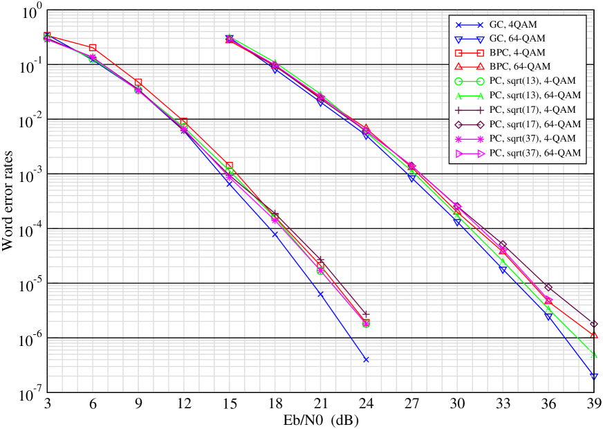
Figure 5: Golden code (GC) (perfect code with $p=5$) and other perfect codes (PC) compared to the best peviously known $2\times 2$ codes (BPC).

In Figure 5, we have plotted the codeword error rates for the Golden code (GC), some other $2\times 2$ Perfect codes (PC) and the best previously known $2\times 2$ STBCs [9] (BPC), as a function of $E_{b}/N_{0}$, using $4,16,64$-QAM constellations. In [9], the values of $\gamma$ giving the best codes were obtained by numerical optimizations and depend on the spectral efficiency. As we concluded in [4, 5], the Golden code has the best performance. We see in Fig. 5 that perfect codes with $p=\sqrt{13}$ and $p=\sqrt{37}$ have performance close to that of the BPCs. However the code with $p=\sqrt{17}$ which is not a perfect code (the cyclic algebra is not a division algebra) has the worst performances, and we can even observe a change in the slope of the curve for high SNR, due to the reduced diversity order of this code ($2$ instead of $4$). In fact, as shown in Example 4, there exists an $x\in K=\mathbb{Q}(i,\sqrt{17})$ such that $N_{K/\mathbb{Q}(i)}(x)=i$. The appearance of such an $x$ is rare, which explains why this code works well at low and medium signal to noise ratio and the change of slope appears at very low error rates.

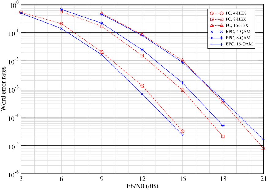
Figure 6: Perfect $3\times 3$ codes with HEX symbols (PC) compared to the best peviously known codes (BPC).

In Fig. 6 and 7, we have plotted respectively the codeword error rates of the $3\times 3$ and the $4\times 4$ PC and the best previously known codes [11, 16] as a function of $E_{b}/N_{0}$. In Fig. 6, we see that for the 4-HEX constellation, the BPC performs a little better than the PC. However, when the constellation is 8-HEX or larger, PCs have better performance, due to the constant minimum determinant.

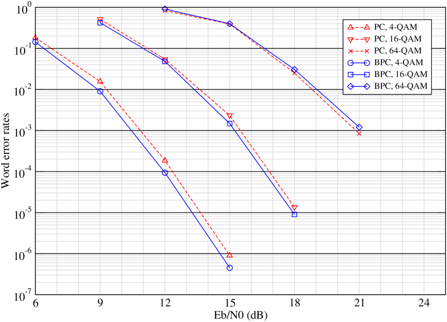
Figure 7: Perfect $4\times 4$ codes with QAM symbols (PC) compared to the best peviously known codes (BPC).

In Fig. 7, we note that the $4\times 4$ PC improves over BPC codes when we use the 64-QAM.

X Conclusion

In this paper we presented new algebraic constructions of full-rate, fully diverse $2\times 2$, $3\times 3$, $4\times 4$ and $6\times 6$ space-time codes, having a constant minimum determinant as the spectral efficiency increases. The name perfect STBC, used for these codes, was suggested by the fact that they satisfy a large number of design criteria and only appear in a few special cases as the classical perfect error correcting codes, achieving the Hamming sphere packing bound.

Appendix A Number Fields: Basic Definitions

The codebooks we build are based on cyclic algebras built over number fields, we thus need some background on number fields. This appendix aims at giving intuition to the reader who does not know the topic. It focuses on examples, and may skip some technical points in order to be more accessible.

Number fields can first be thought of as finite vector spaces over a base field. For example, $\mathbb{Q}(i)=\{a+bi,~{}a,b\in\mathbb{Q}\}$ is a vector space of dimension 2 over $\mathbb{Q}$, whose basis is given by $\{1,i\}$. In our case, we will consider two number fields, denoted by $K$ and $F$, and $K$ will be a vector space of dimension $n$ over $F$. We say that $K$ is a field extension of $F$, which we denote by $K/F$. The dimension of $K$ over $F$ as a vector space is called the degree, and is denoted by $[K:F]$. Another way of thinking of a number field is to add a root of a polynomial, with coefficients in $F$, to a field, and to add also all its powers and multiples, so that the resulting set is indeed a field. For example, $\mathbb{Q}(i)$ is built adding the roots of the polynomial $X^{2}+1$ to $\mathbb{Q}$. The field extension $K/F$ can similarly be seen as adding the element $\theta$, root of a polynomial $p(X)$, to $K$. We may write $K=F(\theta)$. Since a polynomial has $n$ roots, one may wonder if taking one root or another may change the number field. If all the roots are indeed in the number field, it does not change, and the number field is called a Galois extension. Not all number fields are Galois extensions.

For our purpose, we are interested in a field extension $K/F$ such that all roots $\theta_{1},\ldots,\theta_{n}$ of $p(X)$ are not only in $K$, but furthermore are related to each other as follows: there exists a map $\sigma$ such that $\sigma^{k}(\theta_{1})=\theta_{j}$, $k,j=1,\ldots,n$. In such case, $K/F$ is called a cyclic Galois extension, and $\{\sigma^{k}\}$, $k=1,\ldots,n$, is called a (cyclic) Galois group (it can be shown that it has indeed a group structure). For example, $\mathbb{Q}(i)$ is a cyclic Galois extension of degree 2, since there exists $\sigma:i\mapsto-i$.

There are two important objects that can be defined thanks to $\{\sigma^{k}\}$, $k=1,\ldots,n$. We define the trace and the norm of an element $x\in K$ resp. as follows:

$$\mbox{Tr}_{K/F}(x)=\sum_{k=0}^{n-1}\sigma^{k}(x),~{}\mbox{N}_{K/F}(x)=\prod_{k=0}^{n-1}\sigma^{k}(x).$$

We may call a relative trace/norm if the base field is not $\mathbb{Q}$, by opposition to an absolute trace/norm when $F=\mathbb{Q}$.

Let now $L$ be a number field of degree $n$ over $\mathbb{Q}$. Consider the set of elements $x$ of $L$ that satisfy the following property: there exists a monic polynomial $f$ with coefficients in $\mathbb{Z}$ such that $f(x)=0$. This set is called the ring of integers of $L$, and is denoted by $\mathcal{O}_{L}$. It can be shown that this is indeed a ring, but what is more interesting is that this set posseses a $\mathbb{Z}$-basis. We will use this fact extensively in the paper. Let $\{\omega_{1},\ldots,\omega_{n}\}$ be a $\mathbb{Z}$-basis, i.e., all elements can be written as integer linear combinations of basis elements. Then $\det(\mbox{Tr}_{L/\mathbb{Q}}(\omega_{i}\omega_{j})_{i,j=1}^{n})$ is an invariant of $L$ called the discriminant of $L$. Similarly as for the trace and norm, we call the discriminant absolute to emphasize that the base field is $\mathbb{Q}$, and $relative$ otherwise.

Appendix B The Hasse Norm Symbol

In this Appendix, we introduce the Hasse Norm Symbol. It is a tool derived from Class Field Theory, that allows to compute whether a given element is a norm. Our exposition is based on [18]. In the following, we consider extensions of number fields $K/F$ that we assume abelian.

Denote by $K_{\nu}$ the completion of $K$ with respect to the valuation $\nu$. We denote the embedding of $K$ into $K_{\nu}$ by $i_{\nu}$.

Definition 5

[18, p. 105] Let $K/F$ be an abelian extension of number fields with Galois group $\mbox{Gal}(K/F)$. The map

$$\begin{array}[]{clll}\left(\frac{\bullet~{},~{}K/F}{\nu}\right):&K^{*}&\rightarrow&\mbox{Gal}(K/F)\\ &x&\mapsto&\left(\frac{i_{\nu}(x),K/F}{\nu}\right)\end{array}$$

is called the Hasse norm symbol.

The main property of this symbol is that it gives a way to compute whether an element is a local norm [18, p. 106,107].

Theorem 2

We have $\left(\frac{x,K/F}{\nu}\right)=1$ if and only if $x$ is a local norm at $\nu$ for $K/F$.

In order to compute the Hasse norm symbol, we need to know some of its properties. Let us begin with a property of linearity.

Theorem 3

We have

$$\left(\frac{xy,K/F}{\nu}\right)=\left(\frac{x,K/F}{\nu}\right)\left(\frac{y,K/F}{\nu}\right).$$

We then know how the symbol behaves at unramified places [18, p. 106].

Theorem 4

If $\nu$ is unramified in $K/F$, then we have, for all $x\in F^{*}$:

$$\left(\frac{x,K/F}{\nu}\right)=\left(\frac{K/F}{\nu}\right)^{v(x)},$$

where $\left(\frac{K/F}{\nu}\right)$ denotes the Frobenius of $\nu$ for $K/F$ (see Remark 3 below), and $v(x)$ denotes the valuation of $x$.

Remark 3

For our purpose, it is enough to know that the Frobenius $\left(\frac{K/F}{\nu}\right)$ is an element of the Galois group $\mbox{Gal}(K/F)$. We do not need to know it explicitly. For a precise definition, we let the reader refer to [18, p. 107].

Corollary 6

At an unramified place, a unit is always a norm.

Proof:

It is straightforward since the valuation of a unit is 0. ∎

A remarkable property of the Hasse norm symbol is the product formula [18, p. 113].

Theorem 5

Let $K/F$ be a finite extension. For any $x\in F^{*}$ we have:

$$\prod_{\nu}\left(\frac{x,K/F}{\nu}\right)=1,$$

where the product is defined over all places $\nu$.

Remark 4

By Corollary 6, we know that a unit is always a norm locally if the place is unramified. Since we are interested in showing that a unit $\gamma$ is not a norm, we will look for a contradiction at a ramified place.

Before giving the proofs in themselves, we explain briefly their general scheme. The idea is to start from the product formula, and to simplify all the terms except two in the product over all primes, so that we get a product of two terms equal to 1:

$$\left(\frac{\gamma,K/F}{\nu}\right)\left(\frac{x,K/F}{\nu^{\prime}}\right)=1,~{}x\in F^{*}.$$

Hopefully, one of the two terms left will involve $\gamma$, the other will be shown to be different from 1, so that since the product is 1, we will deduce that the term involving $\gamma$ is different from 1, thus $\gamma$ is not a norm. In order to make it easier to simplify the product formula, we introduce an element $y\in K$ such that $y\gamma$ is a unit locally at ramified primes, and we compute the product formula

$$\prod_{\nu}\left(\frac{y\gamma,K/F}{\nu}\right)=1.$$

Appendix C $j$ and $j^{2}$ are not a norm  in $\mathbb{Q}(j,2\cos\left(\frac{2\pi}{7}\right))/\mathbb{Q}(j)$

In this section, we prove that $j$ and $j^{2}$ are a not a norm in $\mathbb{Q}(j,2\cos\left(\frac{2\pi}{7}\right))/\mathbb{Q}(j)$. We show that $j$ and $j^{2}$ are not a norm locally by computing their Hasse norm symbol. The proof is detailed for $j$.

Proposition 10

The unit $j$ is not a norm in $K/F=\mathbb{Q}(j,2\cos\left(\frac{2\pi}{7}\right))/\mathbb{Q}(j)$.

Proof:

We consider the field extension $K/F$. We have

$$7\mathbb{Z}[j]=(j-2)(j+3)=\mathfrak{p}_{7}\mathfrak{q}_{7}.$$

We show that $j$ is not a norm locally in $\mathfrak{p}_{7}$, thus $j$ is not a norm in $K$.

We look for a number $y$ in $\mathbb{Z}[j]$ satisfying

$$y \equiv 1~{}(\mbox{mod }j-2)$$ (21)

$$jy \equiv 1~{}(\mbox{mod }j+3).$$ (22)

By applying the Chinese Remainder Theorem over $\mathbb{Z}[j]$, we find $y=7-3j$ with $(y)\mathbb{Z}[j]=\mathfrak{p}_{79}$. Let $\left(\frac{x,K/F}{\nu}\right)$ denote the Hasse norm symbol. By the product formula

$$\prod_{\nu}\left(\frac{jy,K/F}{\nu}\right)=\prod_{\nu\mbox{ ramified}}\left(\frac{jy,K/F}{\nu}\right)\prod_{\nu\mbox{ unramified}}\left(\frac{jy,K/F}{\nu}\right)=1.$$ (23)

The product on the ramified primes yields $\left(\frac{jy,K/F}{\mathfrak{p}_{7}}\right)\left(\frac{jy,K/F}{\mathfrak{q}_{7}}\right)$, since the ramification in $K/\mathbb{Q}(j)$ is in $7$ only. Note that $\left(\frac{xy,K/F}{\nu}\right)=\left(\frac{x,K/F}{\nu}\right)\left(\frac{y,K/F}{\nu}\right)$ by linearity. We now look at the product on the unramified primes. Since $y\in\mathfrak{p}_{79}$, its valuation is zero for $\nu\neq\mathfrak{p}_{79}$. The valuation of a unit is zero for all places, so that we get

$$\prod_{\nu\mbox{ unramified}}\left(\frac{jy,K/F}{\nu}\right)=\prod_{\nu\mbox{ unramified}}\left(\frac{j,K/F}{\nu}\right)\left(\frac{y,K/F}{\nu}\right)=\left(\frac{y,K/F}{\mathfrak{p}_{79}}\right).$$

Thus equation (23) simplifies to

$$\left(\frac{j,K/F}{\mathfrak{p}_{7}}\right)\left(\frac{y,K/F}{\mathfrak{p}_{7}}\right)\left(\frac{jy,K/F}{\mathfrak{q}_{7}}\right)\left(\frac{y,K/F}{\mathfrak{p}_{79}}\right)=1.$$

The second and third terms are 1 by choice of $y$ (see equations (21) and (22)), so that finally we have

$$\left(\frac{j,K/F}{\mathfrak{p}_{7}}\right)\left(\frac{y,K/F}{\mathfrak{p}_{79}}\right)=1.$$

Since $\mathfrak{p}_{79}$ is inert, the second term is different from 1, so that $\left(\frac{j,K/F}{\mathfrak{p}_{7}}\right)\neq 1$. In words, $j$ is not a norm in $\mathfrak{p}_{7}$ which concludes the proof. ∎

Proposition 11

The unit $j^{2}$ is not a norm in $K/F=\mathbb{Q}(j,2\cos\left(\frac{2\pi}{7}\right))/\mathbb{Q}(j)$.

Proof:

The proof that $j^{2}$ is not a norm is similar to the above one. We keep the notation of the above proof. We show that $j^{2}$ is not a norm locally in $\mathfrak{p}_{7}$, thus $j^{2}$ is not a norm in $K$.
Let $y=5j-9$. We have that

$$y \equiv 1~{}(\mbox{mod }j-2)$$ (24)

$$j^{2}y \equiv 1~{}(\mbox{mod }3+j)$$ (25)

and $(y)\mathbb{Z}[j]=\mathfrak{p}_{151}$. Repeating the same computations as in the above proof, we get

$$\left(\frac{j^{2},K/F}{\mathfrak{p}_{7}}\right)\left(\frac{y,K/F}{\mathfrak{p}_{151}}\right)=1,$$

where $\mathfrak{p}_{151}$ is inert. This implies that $j^{2}$ is not a norm. ∎

Appendix D $i^{2}=-1$ is not a norm in $\mathbb{Q}(i,2\cos(\frac{2\pi}{15}))/\mathbb{Q}(i)$.

We prove here that $i^{2}=-1$ is not a norm in $\mathbb{Q}(i,2\cos(\frac{2\pi}{15}))/\mathbb{Q}(i)$. The general scheme of the proof is the same as in Appendix C, though we have to be a bit more careful here, since the ramification in $\mathbb{Q}(i,2\cos(\frac{2\pi}{15}))/\mathbb{Q}(i)$ appears in two primes, unlike in $\mathbb{Q}(j,2\cos\left(\frac{2\pi}{7}\right))/\mathbb{Q}(j)$.

Proposition 12

The unit -1 is not a norm in $K/F=\mathbb{Q}(i,2\cos(\frac{2\pi}{15}))/\mathbb{Q}(i)$.

Proof:

We consider the field extension $K/F$. We have

$$5\mathbb{Z}[i]=(i+2)(i-2)=\mathfrak{p}_{5}\mathfrak{q}_{5}\mbox{ and }3\mathbb{Z}[i]=3=\mathfrak{p}_{3}.$$

We show that $i$ is not a norm locally in $\mathfrak{p}_{5}$, thus $i$ is not a norm in $K$. We look for a number $y$ in $\mathbb{Z}[i]$ satisfying

$$y \equiv 1~{}(\mbox{mod }i+2)$$ (26)

$$-y \equiv 1~{}(\mbox{mod }i-2)$$ (27)

$$-y \equiv 1~{}(\mbox{mod }3)$$ (28)

By applying the Chinese Remainder Theorem over $\mathbb{Z}[i]$, we find $y=12i-25$ with $(y)\mathbb{Z}[j]=\mathfrak{p}_{769}$. Let $\left(\frac{x,K/F}{\nu}\right)$ denote the Hasse norm symbol. By the product formula

$$\prod_{\nu}\left(\frac{-y,K/F}{\nu}\right)=1.$$ (29)

The product on the ramified primes yields $\left(\frac{-y,K/F}{\mathfrak{p}_{5}}\right)\left(\frac{-y,K/F}{\mathfrak{q}_{5}}\right)\left(\frac{-y,K/F}{\mathfrak{p}_{3}}\right)$, since the ramification in $K/F$ is only in $5$ and $3$. Since $y\in\mathfrak{p}_{769}$, its valuation is zero for $\nu\neq\mathfrak{p}_{769}$. The valuation of a unit is zero for all places, so that we get for the product on the unramified primes

$$\prod_{\nu\mbox{ unramified}}\left(\frac{-y,K/F}{\nu}\right)=\prod_{\nu\mbox{ unramified}}\left(\frac{-1,K/F}{\nu}\right)\left(\frac{y,K/F}{\nu}\right)=\left(\frac{y,K/F}{\mathfrak{p}_{769}}\right).$$

Thus equation (29) simplifies to

$$\left(\frac{-y,K/F}{\mathfrak{p}_{3}}\right)\left(\frac{y,K/F}{\mathfrak{p}_{5}}\right)\left(\frac{-1,K/F}{\mathfrak{p}_{5}}\right)\left(\frac{-y,K/F}{\mathfrak{q}_{5}}\right)\left(\frac{y,K/F}{\mathfrak{p}_{769}}\right)=1.$$

The first, second and fourth terms are 1 by choice of $y$ (see equations (26), (27) and (28)), so that finally we have

$$\left(\frac{-1,K/F}{\mathfrak{p}_{5}}\right)\left(\frac{y,K/F}{\mathfrak{p}_{769}}\right)=1.$$

Since $\mathfrak{p}_{769}$ does not split completely, the second term is different from 1, so that $\left(\frac{-1,K/F}{\mathfrak{p}_{5}}\right)\neq 1$, which concludes the proof.

∎

Appendix E $(-j)^{3}=-1$ is not a norm  in $\mathbb{Q}(j,\zeta_{28}+\zeta_{28}^{-1})/\mathbb{Q}(j)$.

We prove here that $(-j)^{3}=-1$ is not a norm in $\mathbb{Q}(j,\zeta_{28}+\zeta_{28}^{-1})/\mathbb{Q}(j)$. The proof is similar to that of Appendix D.

Proposition 13

The unit -1 is not a norm in $K/F=\mathbb{Q}(\zeta_{28}+\zeta_{28}^{-1},j)/\mathbb{Q}(j)$.

Proof:

We consider the field extension $K/F$. We have

$$7\mathbb{Z}[j]=(j-2)(j+3)=\mathfrak{p}_{7}\mathfrak{q}_{7}\mbox{ and }2\mathbb{Z}[j]=2=\mathfrak{p}_{2}.$$

We show that $-1$ is not a norm locally in $\mathfrak{p}_{7}$, thus $-1$ is not a norm in $K$.

We look for a number $y$ in $\mathbb{Z}[j]$ satisfying

$$y \equiv 1~{}(\mbox{mod }j-2)$$ (30)

$$-y \equiv 1~{}(\mbox{mod }3+j)$$ (31)

$$-y \equiv 1~{}(\mbox{mod }2)$$ (32)

By applying the Chinese Remainder Theorem over $\mathbb{Z}[j]$, we find $y=3-8j$ with $(y)\mathbb{Z}[j]=\mathfrak{p}_{97}$. Let $\left(\frac{x,K/F}{\nu}\right)$ denote the Hasse norm symbol. By the product formula

$$\prod_{\nu}\left(\frac{-y,K/F}{\nu}\right)=1.$$ (33)

The product on the ramified primes yields $\left(\frac{-y,K/F}{\mathfrak{p}_{7}}\right)\left(\frac{-y,K/F}{\mathfrak{q}_{7}}\right)\left(\frac{-y,K/F}{\mathfrak{p}_{2}}\right)$, since the ramification in $K/F$ is in $7$ and $2$ only. Since $y\in\mathfrak{p}_{97}$, its valuation is zero for $\nu\neq\mathfrak{p}_{97}$. The valuation of a unit is zero for all places, so that we get for the product on the unramified primes

$$\prod_{\nu\mbox{ unramified}}\left(\frac{-y,K/F}{\nu}\right)=\prod_{\nu\mbox{ unramified}}\left(\frac{-1,K/F}{\nu}\right)\left(\frac{y,K/F}{\nu}\right)=\left(\frac{y,K/F}{\mathfrak{p}_{97}}\right).$$

Thus equation (33) simplifies to

$$\left(\frac{-y,K/F}{\mathfrak{p}_{2}}\right)\left(\frac{y,K/F}{\mathfrak{p}_{7}}\right)\left(\frac{-1,K/F}{\mathfrak{p}_{7}}\right)\left(\frac{-y,K/F}{\mathfrak{q}_{7}}\right)\left(\frac{y,K/F}{\mathfrak{p}_{97}}\right)=1.$$

The first, second and fourth terms are 1 by choice of $y$ (see equations (30), (31) and (32)), so that finally we have

$$\left(\frac{-1,K/F}{\mathfrak{p}_{7}}\right)\left(\frac{y,K/F}{\mathfrak{p}_{97}}\right)=1.$$

Since $\mathfrak{p}_{97}$ does not split completely, the second term is different from 1, so that $\left(\frac{-1,K/F}{\mathfrak{p}_{7}}\right)\neq 1$, which concludes the proof.

∎

Appendix F The LLL reduction algorithm over $\mathbb{Z}[j]$

The standard LLL reduction algorithm [19] over $\mathbb{Z}$ can be easily modified to work over $\mathbb{Z}[j]$ [23]. The two main points to be careful about are

• the Euclidean division: the quotient of the Euclidean division over $\mathbb{Z}[j]$ is defined as follows: let $x=x_{1}+jx_{2}$ and $y=y_{1}+jy_{2}$, $x_{1},x_{2},y_{1},y_{2}\in\mathbb{Z}$. The division of $x$ by $y$ yields $\frac{x}{y}=z_{1}+jz_{2}$, with $z_{1},z_{2}\in\mathbb{Q}$. Then we have that $x=yq+r$, where $q=[z_{1}]+j[z_{2}]$.

• the conjugation: the usual complex conjugation is replaced by the $\tau$-conjugation, that sends $j$ onto $j^{2}$.

$$\begin{diagram}$$

Figure 1: The compositum of a totally real field $\mathbb{Q}(\theta)$ and $F=\mathbb{Q}(i)$ or $\mathbb{Q}(j)$ with coprime discriminants: relative degrees are shown on the branches.

Figure 2: 4-HEX Constellation.

Figure 3: 8-HEX Constellation.

Figure 4: 16-HEX Constellation.

References

- [1] E. Bayer, F. Oggier, and E. Viterbo, “New algebraic constructions of rotated lattice constellations for the Rayleigh fading channel,” IEEE Trans. Inform. Theory, April 2004.
- [2] E. Bayer, F. Oggier, and E. Viterbo, “Algebraic lattice constellations: Bounds on performance,” IEEE Trans. on Inf. Theory, vol. 52, no 1, Jan 2006.
- [3] J.-C. Belfiore and G. Rekaya, “Quaternionic lattices for space-time coding,” in Proceedings of the Information Theory Workshop, IEEE, Paris 31 March - 4 April 2003 ITW 2003.
- [4] J.-C. Belfiore, G. Rekaya, and E. Viterbo, “The Golden Code: A full rate Space-Time Code with non vanishing Determinants,” in Proceedings 2004 IEEE International Symposium on Information Theory, IEEE I. T. Society, June 27- July 2 2004.
- [5] J.-C. Belfiore, G. Rekaya, and E. Viterbo, “The Golden Code: A full rate Space-Time Code with non vanishing Determinants,” IEEE Trans. on Inf. Theory, vol. 51, no 4, April 2005.
- [6] H. Cohn, Advanced Number Theory. Dover Publications Inc. New York, 1980.
- [7] J. H. Conway and N. J. A. Sloane, Sphere Packings, Lattices and Groups. Grundlehren der mathematischen Wissenschaften, New York Berlin: Springer-Verlag, 2 ed., 1988.
- [8] M. O. Damen, A. Chkeif, and J.-C. Belfiore, “Lattice codes decoder for space-time codes,” IEEE Commun. Lett., vol. 4, pp. 161–163, May 2000.
- [9] M. O. Damen, A. Tewfik, and J.-C. Belfiore, “A construction of a space-time code based on the theory of numbers,” IEEE Trans. Inform. Theory, vol. 48, pp. 753–760, March 2002.
- [10] P. Dayal and M. K. Varanasi, “An optimal two transmit antenna Space-Time Code and its stacked extensions,” in Proc. Asilomar Conf. on Signals, Systems and Computers, Monterey, CA, November 2003.
- [11] H. El Gamal and M. O. Damen, “Universal space-time coding,” IEEE Trans. Inform. Theory, vol. 49, pp. 1097–1119, May 2003.
- [12] H. El Gamal and A. R. Hammons Jr., “A new approach to layered space-time coding and signal processing,” IEEE Trans. Inform. Theory, vol. 47, pp. 2321–2334, September 2001.
- [13] P. Elia, K. Raj Kumar, S. A. Pawar, P. Vijay Kumar and H.-F. Lu, “Explicit, Minimum-Delay Space-Time Codes Achieving The Diversity-Multiplexing Gain Tradeoff,” Submitted to IEEE Trans. Inform. Theory, Sept. 2004.
- [14] G. D. Forney, Jr, R. G. Gallager, G. R. Lang, F. M. Longstaff, and S. U. Qureshi, “Efficient modulation for band-limited channels,” IEEE J. Select. Areas Commun., vol. 2, pp. 632–647, September 1984.
- [15] A. Fröhlich and M. Taylor, Algebraic number theory. Cambridge University Press, 1991.
- [16] S. Galliou and J.-C. Belfiore, “A new family of full rate, fully diverse space-time codes based on Galois theory,” in Proceedings IEEE International Symposium on Information Theory, p. 419, IEEE, June 30-July 5 2002.
- [17] F. Q. Gouv a, p-adic numbers: An introduction. Universitext, Springer, second ed., 1997.
- [18] G. Gras, Class Field Theory. Springer Verlag, 2003.
- [19] M. Gr tschel, L. Lovász, and A. Schrijver, Geometric Algorithms and Combinatorial Optimization. New York: Springer-Verlag, 1988.
- [20] B. Hassibi and H. Vikalo, “On sphere decoding algorithm. I. Expected complexity”, IEEE Transactions on Signal Processing, vol. 53, no. 8, August 2005, pp. 2806 - 2818.
- [21] B. Hassibi and B. M. Hochwald, “High-rate codes that are linear in space and time,” IEEE Trans. Inform. Theory, vol. 48, pp. 1804–1824, July 2002.
- [22] Liedl and Niederreiter, Finite Fields and its applications.
- [23] H. Napias, “A generalization of the LLL algorithm over Euclidean rings or orders,” Journal de Th orie des Nombres de Bordeaux, vol. 8, pp. 387–396, 1996.
- [24] F. Oggier and E. Viterbo, “Algebraic number theory and code design for Rayleigh fading channels”, Foundations and Trends in Communications and Information Theory, vol. 1, 2004.
- [25] P. Samuel, Algebraic number theory (Original Title in French: Th orie Alg brique des nombres). Méthodes, Hermann, 2 ed., 2003.
- [26] W. Scharlau, Quadratic and Hermitian Forms. Springer Verlag, 1985.
- [27] A. Schiemann, “Classification of hermitian forms with the neighbour method,” J. Symbolic Computation, vol. 26, pp. 487–508, 1998.
- [28] B. A. Sethuraman, B. S. Rajan, and V. Shashidhar, “Full-diversity, high-rate space-time block codes from division algebras,” IEEE Trans. Inform. Theory, vol. 49, pp. 2596– 2616, October 2003.
- [29] G. Rekaya and J.-C. Belfiore, “On the complexity of ML lattice decoders for decoding linear full-rate space-time codes,” in Proceedings 2003 IEEE International Symposium on Information Theory, ISIT Yokohama, July 2003.
- [30] H. P. F. Swinnerton-Dyer, A brief guide to algebraic number theory. Cambridge University Press, 2001.
- [31] V. Tarokh, N. Seshadri, and A. Calderbank, “Space-time codes for high data rate wireless communication : Performance criterion and code construction,” IEEE Trans. Inform. Theory, vol. 44, pp. 744–765, March 1998.
- [32] E. Viterbo and J. Boutros: “A Universal Lattice Code Decoder for Fading Channels,” IEEE Transactions on Information Theory, vol. 45, n. 5, pp. 1639–1642, July 1999.
- [33] H. Yao and G. W. Wornell, “Achieving the full MIMO diversity-multiplexing frontier with rotation-based space-time codes,” in Proceedings Allerton Conf. Commun., Cont., and Computing, (Illinois), October 2003.
- [34] L. Zheng, D. Tse, “Diversity and Multiplexing: A Fundamental Tradeoff in Multiple-Antenna Channels,” IEEE Trans. on Information Theory, vol. 49, no. 5, pp. 1073-1096, May 2003.
- [35] M. Pohst,“KASH/KANT-computer algebra system.” Technische Universität, Berlin, available at http://www.math.tu-berlin.de/algebra/.