Nearly optimal exploration-exploitation decision thresholds

Abstract

While in general trading off exploration and exploitation in reinforcement learning is hard, under some formulations relatively simple solutions exist. In this paper, we first derive upper bounds to for the utility of selecting different actions in the multi-armed bandit setting. Unlike the common statistical upper confidence bounds, these explicitly link the planning horizon, uncertainty and the need for exploration explicit. The resulting algorithm can be seen as a generalisation of the classical Thompson sampling algorithm. We experimentally test these algorithms, as well as $\epsilon$-greedy and the value of perfect information heuristics. Finally, we also introduce the idea of bagging for reinforcement learning. By employing a version of online bootstrapping, we can efficiently sample from an approximate posterior distribution.

1 Introduction

In reinforcement learning, the dilemma between selecting actions to maximise the expected return according to the current world model and to improve the world model such as to potentially be able to achieve a higher expected return is referred to as the exploration-exploitation trade-off. This has been the subject of much interest before, one of the earliest developments being the theory of sequential sampling in statistics, as developed by [1]. This dealt mostly with making sequential decisions for accepting one among a set of particular hypothesis, with a view towards applying it to jointly decide the termination of an experiment and the acceptance of a hypothesis. A more general overview of sequential decision problems from a Bayesian viewpoint is offered in [2].

The optimal, but intractable, Bayesian solution for bandit problems was given in [3], while recently tight bounds on the sample complexity of exploration have been found [4]. An approximation to the full Bayesian case for the general reinforcement learning problem is given in [5], while an alternative technique based on eliminating actions which are confidently estimated as low-value is given in [6].

As will be seen in the next section, the intuitive concept of trading exploration and exploitation is a natural consequence of the definition of the problem of reinforcement learning. Our first contribution is to see show in Sec. 3 that there is a simple threshold for switching from exploratory to greedy behaviour in bandit problems. This threshold is found to depend on the effective reward horizon of the optimal policy and on our current belief distribution of the expected rewards of each action. A sketch of the extension to MDPs is presented in Sec. 4, while Sec. 5 derives an upper bound on the value of exploration to derive practical algorithms. Section 6 introduces the use of online bootstrapping for reinforcement learning, in order to approximate sampling for posterior distributions. Finally, the resulting algorithms are then illustrated experimentally in Sec. 7. We conclude with a discussion on the relations with other methods.

2 Exploration Versus Exploitation

Let us assume a standard multi-armed bandit setting, where a reward distribution $p(r_{t+1}|a_{t})$ is conditioned on actions in $a_{t}\in{\mathcal{A}}$, with $r_{t}\in{\mathbb{R}}$. The aim is to discover a policy $\pi=\{P(a_{t}=i)|i\in{\mathcal{A}}\}$ for selecting actions such that $E[r_{t+1}|\pi]$ is maximised. It follows that the optimal gambler, or oracle, for this problem would constitute a policy which always chooses $i\in{\mathcal{A}}$ such that $E[r_{t+1}|a_{t}=i]\geq E[r_{t+1}|a_{t}=j]$ for all $j\in{\mathcal{A}}$. Given the conditional expectations, implementing the oracle is trivial. However this tells us little about the optimal way to select actions when the expectations are unknown. As it turns out, the optimal action selection mechanism will depend upon the problem formulation. We initially consider the two simplest cases in order to illustrate that the exploration/exploitation tradeoff is and should be viewed in terms of problem and model definition.

In the first problem formulation the objective is to discover a parameterized probabilistic policy $\pi=\big{\{}P(a_{t}|\theta_{t})~{}\big{|}~{}a_{t}\in{\mathcal{A}}\big{\}}$, with parameters $\theta_{t}$, for selecting actions such that $E[r_{t+1}|\pi]$ is maximised. If we consider a model whose parameters are the set of estimates $\theta_{t}=\big{\{}q_{i}=\hat{E}_{t}[r_{t+1}|a_{t}=i]~{}\big{|}~{}i\in{\mathcal{A}}\big{\}}$, then the optimal choice is to select $a_{t}$ for which the estimated expected value of the reward is highest, because according to our current belief any other choice will necessarily lead to a lower expectation. Thus, stating the bandit problem in this way does not allow the exploration of seemingly lower, but potentially higher value actions and it results in a greedy policy.

In the second formulation, we wish to minimise the discrepancy between our estimate $q_{i}$ and the true expectation. This could be written as the following minimisation problem:

$$\sum_{i\in{\mathcal{A}}}E\big{[}\|r_{t+1}-q_{i}\|^{2}~{}\big{|}~{}a_{t}=i\big{]}.$$

For point estimates of the expected reward, this requires sampling uniformly from all actions and thus represents a purely exploratory policy. If the problem is stated as simply minimising the discrepancy asymptotically, then uniformity is not required and it is only necessary to sample from all actions infinitely often. This condition holds when $P(a_{t}=i)>0~{}\forall i\in{\mathcal{A}},~{}t>0$ and can be satisfied by mixing the optimal policies for the two formulations, with a probability $\epsilon$ of using the uniform action selection and a probability $1-\epsilon$ of using the greedy action selection. This results in the well-known $\epsilon$-greedy policy (see for example [7]), with the parameter $\epsilon\in[0,1]$ used to control exploration.

This formulation of the exploration-exploitation problem, though leading to an intuitive result, does not lead to an obvious way to optimally select actions. In the following section we shall consider bandit problems for which the functional to be maximised is

$$E\bigg{[}\sum_{k=0}^{N}g(k)r_{t+k+1}\bigg{|}\pi\bigg{]},\quad g(k)\in[0,1],~{}N\geq 0,$$

with $\sum_{k=0}^{\infty}g(k)<\infty$. In this formulation of the problem we are not only interested in maximising the expected reward at the next time step, but in the subsequent $N$ steps, with the $g(\cdot)$ function providing another convenient way to weigh our preference among short and long-term rewards. Intuitively it is expected that the optimal policy for this problem will be different depending on how long-term are the rewards that we are interested in. As will be shown later, by lengthening the effective reward horizon through manipulation of $g$ and $N$, i.e. by changing the definition of the problem that we wish to solve, the exploration bias is increased automatically.

3 Optimal Exploration Threshold for Bandit Problems

We want to know when it is a better decision to take action $i$ rather than some other action $j$, with $i,j\in{\mathcal{A}}$, given that we have estimates $q_{i},q_{j}$ for $E[r_{t+1}|a_{t}=i]$ and $E[r_{t+1}|a_{t}=j]$ respectively. We shall attempt to see under which conditions it is better to take an action different than the one whose expected reward is greatest. For this we shall need the following assumption:

Assumption 1 (Expected rewards are bounded from below)

There exists $b\in{\mathbb{R}}$ such that

$$E[r_{t+1}|a_{t}=i]\geq b\quad\forall~{}i\in{\mathcal{A}},$$ (1)

The above assumption is necessary for imposing a lower bound on the expected return of exploratory actions: no matter what action is taken, we are guaranteed that $E[r_{t}]>b$. Without this condition, exploratory actions would be too risky to be taken at all.

Given two possible actions to take, where one action is currently estimated to have a lower expected reward than the other, then it might be worthwhile to pursue the lower-valued action if the following conditions are true: (a) there is a degree of uncertainty such that the lower-valued action can potentially be better than the higher-valued one, (b) we are interested in maximising more than just the expectation of the next reward, but the expectation of a weighted sum of future rewards, (c) we will be able to accurately determine whether one action is better than the other quickly enough, so that not a lot of resources will be wasted in exploration .

We now start viewing $q_{i}$ as random variables for which we hold belief distributions $p(q_{i})$, with $\bar{q_{i}}=E[q_{i}]=\hat{E}[r_{t+1}|a_{t}=i]$. The problem can be defined as deciding when action $i$, is better than taking action $j$, under the condition that doing so allows us to determine whether $q_{i}>q_{j}+\delta$ with high probability after $T\geq 1$ exploratory actions. For this reason we will need the following bound on the expected return of exploration.

Lemma 1 (Exploration bound)

For any return of the form $R_{t}=\sum_{k=0}^{N}g(k)r_{t+k+1}$, with $g(k)\geq 0$, assuming (1) holds, the expected return of taking action $i$ for $T$ time-steps and following a greedy policy thereafter, when $\bar{q_{i}}>\bar{q_{j}}$, is bounded below by

$$U(i,j,T,\delta,b)=\sum_{k=T}^{N}g(k)\big{(}(\bar{q_{j}}+\delta)P(q_{i}>q_{j}+\delta)+\bar{q_{j}}P(q_{i}\leq q_{j}+\delta)\big{)}\\ +\sum_{k=0}^{T-1}g(k)\big{(}(\bar{q_{j}}+\delta)P(q_{i}>q_{j}+\delta)+bP(q_{i}\leq q_{j}+\delta)\big{)}$$ (2)

for some $\delta>0$.

This follows immediately from Assumption 1. The greedy behaviour supposes we are following a policy where we continue to perform $i$ if we know that $P(q_{i}>q_{j}+\delta)\approx 1$ after $T$ steps and switch back to $j$ otherwise.

Without loss of generality, in the sequel we will assume that $b=0$ (If expected rewards are bounded by some $b\neq 0$, we can always subtract $b$ from all rewards and obtain the same). For further convenience, we set $p_{i}=P(q_{i}\geq q_{j}+\delta)$. Then we may write that we must take action $i$ if the expected return of simply taking action $j$ is smaller than the expected return of taking action $i$ for $T$ steps and then behaving greedily, i.e. if the following holds:

$$\sum_{k=0}^{N}g(k)\bar{q_{j}} <\sum_{k=T}^{N}g(k)\big{(}(\bar{q_{j}}+\delta)p_{i}+\bar{q_{j}}(1-p_{i})\big{)}+\sum_{k=0}^{T-1}g(k)(\bar{q_{j}}+\delta)p_{i}$$ (3)

$$\sum_{k=0}^{T-1}g(k)\big{(}\bar{q_{j}}-(\bar{q_{j}}+\delta)p_{i}\big{)} <\sum_{k=T}^{N}g(k)\big{(}\delta p_{i}\big{)}$$ (4)

Let $g(k)=\gamma^{k}$, with $\gamma\in[0,1]$. In this case, any choice of $T$ can be made equivalent to $T=1$ by dividing everything with $\sum_{k=0}^{T-1}\gamma^{k}$. We explore two cases: $\gamma<1,~{}N\rightarrow\infty$ and $\gamma=1,~{}N<\infty$. In the first case, which corresponds to infinite horizon exponentially discounted reward maximisation problems, we obtain the following:

$$\bar{q_{j}}-(\bar{q_{j}}+\delta)p_{i} <\sum_{k=1}^{\infty}\gamma^{k}\delta p_{i}$$ (5)

$$\frac{\bar{q_{j}}-(\bar{q_{j}}+\delta)p_{i}}{(1-p_{i})\bar{q_{j}}} <\gamma.$$ (6)

It possible to simplify this expression considerably. When $P(q_{i}\geq\bar{q_{j}}+\delta)=1/2$, it follows from (6) that

$$\gamma>\frac{\bar{q_{j}}-(\bar{q_{j}}+\delta)/2}{\bar{q_{j}}/2}=\frac{\bar{q_{j}}-\delta}{\bar{q_{j}}}.$$ (7)

Thus, for infinite horizon discounted reward maximisation problems, when it is known that the all expected rewards are non-negative, all we need to do is find $\delta$ such that $P(q_{i}\geq q_{j}+\delta)=1/2$. Then (7) can be used to make a decision on whether it is worthwhile to perform exploration. Although it might seem strange the $q_{i}$ is omitted from this expression, its value is implicitly expressed through the value of $\delta$.

In the second case, finite horizon cumulative reward maximisation problems, exploration should be performed when the following condition is satisfied:

$$N\delta p_{i} >\bar{q_{j}}-(\bar{q_{j}}+\delta)p_{i}$$ (8)

Here the decision making function is of a different nature, since it depends on both estimates. However, in both cases, the longer the effective horizon becomes and the larger the uncertainty is, the more the bias towards exploration is increased. We furthermore note that in the finite horizon case, the backward induction procedure can be used to make optimal decisions (see [2] Sec. 12.4).

3.1 Solutions for Specific Distributions

If we have a specific form for the distribution $P(q_{i}>q_{j}+\delta)$ it may be possible to obtain analytical solutions. To see how this can be achieved, consider that from (6), we have:

$$\gamma\bar{q_{j}} >\bar{q_{j}}-\delta\frac{p_{i}}{1-p_{i}}$$

$$0 <\delta\frac{P(q_{i}>q_{j}+\delta)}{1-P(q_{j}>q_{j}+\delta)}-(1-\gamma)\bar{q_{j}},$$ (9)

recalling that all mean rewards are non-negative.

If this condition is satisfied for some $\delta$ then exploration must be performed. We observe that if the first term is maximised for some $\delta^{*}$ for which the inequality is not satisfied, then there is no $\delta\neq\delta^{*}$ that can satisfy it. Thus, we can attempt to examine some distributions for which this $\delta^{*}$ can be determined. We shall restrict ourselves to distributions that are bounded below, due to Assumption 1.

3.2 Solutions for the Exponential Distribution

One such distribution is the exponential distribution, defined as

$$P(X>\delta)=\int_{\delta}^{\infty}\beta e^{-\beta(x-\mu)}dx=e^{-\beta(\delta-\mu)}$$

if $\delta>\mu$, 1 otherwise. We may plug this into (9) as follows

$$f(\delta)=\delta\frac{P(q_{i}>q_{j}+\delta)}{1-P(q_{i}>q_{j}+\delta)}=\delta\frac{e^{-\beta_{i}(\mu_{j}+\delta-\mu_{i})}}{1-e^{-\beta_{i}(\mu_{j}+\delta-\mu_{i})}}=\frac{\delta}{e^{\beta_{i}(\mu_{j}+\delta-\mu_{i})}-1}$$

Now we should attempt to find $\delta^{*}=\mathop{\rm arg\,max}_{\delta}f(\delta)$. We begin by taking the derivative with respect to $\delta$. Set $g(\delta)=e^{h(\delta)}-1$, $h(\delta)=\beta_{i}(\bar{q_{j}}+\delta-\mu_{i})$

$$\nabla f(\delta) =\frac{g(\delta)-\delta\nabla g(\delta)}{g(\delta)^{2}}=\frac{g(\delta)-\delta\beta_{i}\nabla_{h}g(\delta)}{g(\delta)^{2}}=\frac{e^{h(\delta)}(1-\delta\beta_{i})-1}{(e^{h(\delta)}-1)^{2}}$$

Necessary and sufficient conditions for some point $\delta^{*}$ to be a local maximum for a continuous differentiable function $f(\delta)$ are that $\nabla_{\delta}f(\delta^{*})=0$ and $\nabla_{\delta}^{2}f(\delta^{*})<0$. The necessary condition for $\delta$ results in

$$e^{\beta_{i}(q_{k}+\delta-\mu_{i})}(1-\delta\beta_{i})=1.$$ (10)

Unfortunately (10) has no closed form solution, but it is related to the Lambert W function for which iterative solutions do exist [8]. The found solution can then be plugged into (9) to see whether the conditions for exploration are satisfied.

4 Extension to the General Case

In the general reinforcement learning setting, the reward distribution does not only depend on the action taken but additionally on a state variable. The state transition distribution is conditioned on actions and has the Markov property. Each particular task within this framework can be summarised as a Markov decision process:

Definition 1 (Markov decision process)

A Markov decision process is defined by a set of states ${\mathcal{S}}$, a set of actions ${\mathcal{A}}$, a transition distribution ${\mathfrak{T}}(s^{\prime},s,a)=P(s_{t+1}^{\prime}|s_{t}=s,a_{t}=a)$ and a reward distribution ${\mathfrak{R}}(s^{\prime},s,a)=p(r_{t+1}|s_{t+1}=s^{\prime},s_{t}=s,a_{t}=a)$.

The simplest way to extend the bandit case to the more general one of MDPs is to find conditions under which the latter reduces to the former. This can be done for example by considering choices not between simple actions but between temporally extended actions, which we will refer to as options following [9]. We shall only need a simplified version of this framework, where each possible option $x$ corresponds to some policy $\pi^{x}:{\mathcal{S}}\times{\mathcal{A}}\to[0,1]$. This is sufficient for sketching the conditions under which the equivalence arises.

In particular, we examine the case where we have two options. The first option is to always select actions according to some exploratory principle, such picking them from a uniform distribution. The second is to always select actions greedily, i.e. by picking the action with the highest expected return.

We assume that each option will last for time $T$. One further necessary component for this framework is the notion of mixing time

Definition 2 (Exploration mixing time)

We define the exploration mixing time for a particular MDP ${\mathcal{M}}$ and a policy $\pi$ $T_{\epsilon}({\mathcal{M}},\pi)$ as the expected number of time steps after which the state distribution is close to the stationary state distribution of $\pi$ after we have taken an exploratory action $i$ at time step $t$, i.e. the expected number of steps $T$ such that the following condition holds:

$$\frac{1}{\|{\mathbb{S}}\|}\sum_{s}\|P(s_{t+T}=s|s_{t},\pi)-P(s_{t+T}=s|a_{t}=i,s_{t},\pi)\|<\epsilon$$

It is of course necessary for the MDP to be ergodic for this to be finite. If we only consider switching between options at time periods greater than $T_{\epsilon}({\mathcal{M}},\pi)$, then the option framework’s roughly corresponds to the bandit framework, and $T_{\epsilon}$ in the former to $T$ in the latter. This means that whenever we take an exploratory action $i$ (one that does not correspond to the action that would have been selected by the greedy policy $\pi$), the distribution of states would remain to be significantly different from that under $\pi$ for $T_{\epsilon}({\mathcal{M}},\pi)$ time steps. Thus we could consider the exploration to be taking place during all of $T_{\epsilon}$, after which we would be free to continue exploration or not. Although there is no direct correspondence between the two cases, this limited equivalence could be sufficient for motivating the use of similar techniques for determining the optimal exploration exploitation threshold in full MDPs.

5 Optimistic Evaluation

In order to utilise Lemma 1 in a practical setting we must define $T$ in some sense. The simplest solution is to set $T=1$, which results in an optimistic estimate for exploratory actions as will be shown below. By rearranging (2) we have

$$U(i,j,T,\delta,b) =\sum_{k=0}^{N}g(k)\bar{q_{j}}+\sum_{k=0}^{N}g(k)\delta p_{i}+(1-p_{i})\left(\sum_{k=0}^{T-1}g(k)(b-\bar{q_{j}}))\right)$$ (11)

from which it is evident, since $q_{j}\geq b$ and $g(k)\geq 0$, that $U(i,j,T_{1},\delta,b)\geq U(i,j,T_{2},\delta,b)$ when $T_{1}<T_{2}$, thus $U(i,j,1,\delta,b)\geq U(i,j,T,\delta,b)$ for any $T\geq 1$. This can now be used to obtain Alg. 1 for optimistic exploration.

Nevertheless, testing for the existence of a suitable $\delta$ can be costly since, barring an analytic procedure it requires an exhaustive search. On the other hand, it may be possible to achieve a similar result through sampling for different values of $\delta$. Herein, the following sampling method is considered: Firstly, we determine the action $j$ with the greatest $\bar{q_{j}}$. Then, for each action $i$ we take a sample $x$ from the distribution $p(q_{i})$ and set $\delta=x-\bar{q_{j}}$. This is quite an arbitrary sampling method, but we may expect to obtain a $\delta>0$ with high probability if $i$ has a high probability to be significantly better than $j$. This method is summarised in Alg. 2.

Algorithm 1 Optimistic exploration

  if $\exists~{}\delta~{}:~{}U(i,j,1,\delta,b)>\sum_{k=0}^{N}g(k)\bar{q_{j}}$ then

     $a\Leftarrow i$

  else

     $a\Leftarrow j$

  end if

Algorithm 2 Optimistic stochastic exploration

  $j\Leftarrow\mathop{\rm arg\,max}_{i}\bar{q_{i}}$.

  $u_{j}=\sum_{k=0}^{N}g(k)\bar{q_{j}}$.

  for all $i\neq j$ do

     $\delta\Leftarrow x-\bar{q_{j}},\quad x\sim p(q_{i})$

     $u_{i}\Leftarrow U(i,j,1,\delta,b)$

  end for

  $a\Leftarrow\mathop{\rm arg\,max}_{i}u_{i}$

Algorithm 3 Thompson sampling

  $a\Leftarrow i$ with probability $P(a=i)=P(q_{i}>q_{j})~{}\forall j\neq i$

An alternative exploration method is given by Alg. 3, first introduced in[10], which samples each action with probability equal to the probability that its expected reward is the highest. It can perhaps be viewed as an approximation to Alg. 2 when $\gamma\rightarrow 1$ and has the advantage that it is extremely simple. However, both of these algorithms require us to be able to sample from the posterior distribution, something that may not always be feasible. For that reason, in the next section we introduce the idea of online bootstrap for reinforcement learning.

6 Online Bootstrapping for reinforcement learning

The algorithms we consider require sampling from a posterior distribution. However, there are two main problems associated with this requirement. Firstly, calculating posterior distributions and sampling from them may be computationally demanding. Secondly, the Bayesian framework requires specifying some prior distribution, and it may not always be clear what this should be. Even when we simply wish to estimate reward distributions, for example, without specific domain knowledge it is not easy to make a choice between standard conjugate prior distributions such as the Beta and Normal-Gamma. While this latter problem can be alleviated by using a hierarchical prior, or a non-parametric approach, this paper proposes a simpler solution: using online bootstrap samples to approximate posteriors.

For bandit problems in particular, we maintain a population of $K$ point estimates for the expected reward of each arm $i$, so that at time $t$ the $k$-th estimate is $q_{i}^{k}(t)$. The initial values $q_{j}^{i}(0)$ are drawn i.i.d. from an appropriate prior distribution. Then, at each step $t$, we draw $k_{t}$ uniformly from $\{1,K\}$ and then use $q_{i}^{k_{t}}(t)$ as our mean reward for both optimistic stochastic exploration and Thompson sampling. Finally, we perform online bootstrapping using

$$q_{a_{t}}^{k_{t}}(t)=(1-\alpha_{t}^{k})q_{a_{t}}^{k_{t}}(t-1)+(1-\alpha_{t}^{k})r_{t}.$$ (12)

If $\alpha_{t}^{k}=\alpha_{t}$ for all $k$, then the only diversity in the population estimate will be due to the initial values. Randomising $\alpha_{t}^{k}$ in such a way that the same conditions for convergence hold will ensure that population diversity will be maintained in a way that reflects uncertainty due to the data. Although we only applied this algorithm for bandit problems, it is also possible to apply it to the transition kernel or value function for the full reinforcement learning problem. However, care should be taken to avoid problems with correlations in the bootstrap samples. It is probably to difficult to apply this technique to non-episodic problems in particular, without domain-specific knowledge.

7 Experiments

A small experiment was performed on a $n$-armed bandit problem with rewards $r_{t}\in\{0,1\}$ drawn from a Bernoulli distribution. Alg. 2 was used with $g(k)=\gamma^{k}$ and $b=0$, which is in agreement with the distribution. This was compared with Alg. 3, which can be perhaps viewed as a crude approximation to Alg. 2 when $\gamma\rightarrow 1$. The performance of $\epsilon$-greedy action selection with $\epsilon=0.01$ was evaluated for reference.

The $\epsilon$-greedy algorithm used point estimates for $\bar{q}_{i}$, which were updated with gradient descent with a step size of $\alpha=0.01$, such that for each action-reward observation tuple $(a_{t}=i,r_{t+1})$, $\bar{q}_{i}\Leftarrow\alpha(r_{t+1}-\bar{q}_{i})$, with initial estimates being uniformly distributed in $[0,1]$. In the other two cases, the complete distribution of $q_{i}$ was maintained via a population $\{p_{i}^{k}\}_{k=0}^{K}$ of point estimates, with $K=16$. Each point estimate in the population was maintained in the same manner as the single point estimates in the $\epsilon$-greedy approach. Sampling actions was performed by sampling uniformly from the members of the population for each action.

The results for two different bandit tasks, one with 16 and the other with 128 arms, averaged over 1,000 runs, are summarised in Fig. 1. For each run, the expected reward of each bandit was sampled uniformly from $[0,1]$.

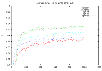
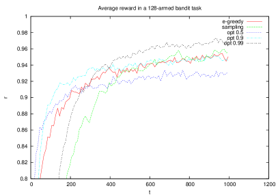
Figure 1: Average reward in an multi-armed bandit task averaged over 1,000 experiments, smoothed with a moving average over 10 time-steps. Results are shown for $\epsilon$-greedy (e-greedy), Thompson sampling (sampling) and Alg. 2 (opt) with $\gamma\in\{0.5,0.9,0.99\}$.

As can be seen from the figure, the $\epsilon$-greedy approach performs relatively well when used with reasonable first initial estimates. The Thompson sampling approach, while having apprximately the same complexity, appears to perform better asymptotically. More importantly, Alg. 2 exhibits better long-term versus short-term performance when the effective reward horizon is increased as $\gamma\rightarrow 1$, which means that the algorithm does manage to take into account the horizon when deciding how to explore.

Finally, we show results for a bandit task with 256 arms, averaged over 1,000 runs, in comparison with the $E^{3}$ and VPI algorithms in Fig. 2.

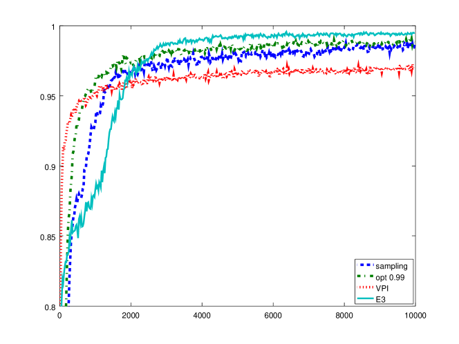
Figure 2: Average reward in an multi-armed bandit task averaged over 1,000 experiments, smoothed with a moving average over 10 time-steps. Results are shown for Thompson sampling (sampling) and Alg. 2 (opt), VPI VPI and $E^{3}$ (E3).

There, we can see that the optimistic sampling approach clearly dominates Thompson sampling, at least under the bootstrap distribution used. Only $E^{3}$ has better asymptotic performance in this task

8 Discussion and Conclusion

This paper has presented a formulation of an optimal exploration-exploitation threshold for in a $n$-armed bandit task, which links the need for exploration to the effective reward horizon and model uncertainty. Additionally, a practical algorithm, based on an optimistic bound on the value of exploration, is introduced. Experimental results show that this algorithm exhibits the expected long-term versus short-term performance trade-off when the effective reward horizon is increased.

While the above formulation fits well within a reinforcement learning framework, other useful formulations may exist. In budgeted learning, any exploratory action results in a fixed cost. Such a formulation is used in [11] for the bandit problem (see also [12] for the active learning case). Then the problem essentially becomes that of how to best sample from actions in the next $T$ moves such that the expected return of the optimal policy after $T$ moves is maximised and corresponds to $g(k)=0~{}\forall k<T$ in the framework presented in this paper. A further alternative, described in [6], is to stop exploring those parts of the state-action space which lead to sub-optimal returns with high probability.

When a distribution or a confidence interval is available for expected returns, it is common to use the optimistic side of the confidence interval for action selection [13]. This practice can be partially justified through the framework presented herein, or alternatively, through considering maximising the expected information to be gained by exploration, as proposed by [14]. In a similar manner, other methods which represent uncertainty as a simple additive factor to the normal expected reward estimates, acquire further meaning when viewed through a statistical decision making framework. For example the Dyna-Q+ algorithm (see [7] chap. 9) includes a slowly increasing exploration bonus for state-action pairs which have not been recently explored. From a statistical viewpoint, the exploration bonus corresponds to a model of a non-stationary world, where uncertainty about past experiences increases with elapsed time elapsed.

In general, the conditions defined in Sec. 3 require maintaining some type of belief, int the form of a distribution, over the expected return of actions. A natural choice for this would be to use a fully analytical Bayesian framework. Unfortunately this makes it more difficult to calculate $P(q_{i}>d)$, so it might be better to consider simple numerical approaches from the outset, such as the bootstrap ones proposed in this paper. We have previously considered some simple such estimates in [15], where we relied on estimating the gradient of the expected return with respect to the parameters. The estimated gradient was then used as a measure of uncertainty. Further results on the use of ensemble estimates for reinforcement learning, and comparisons between various forms of bootstrapping with particle filters and analytical Bayesian estimates can be found in a longer version of this paper in [16].

References

- [1] Wald, A.: Sequential Analysis. John Wiley & Sons (1947) Republished by Dover in 2004.
- [2] DeGroot, M.H.: Optimal Statistical Decisions. John Wiley & Sons (1970)
- [3] Bellman, R.E.: A problem in the sequential design of experiments. Sankhya 16 (1957) 221–229
- [4] Mannor, S., Tsitsiklis, J.N.: The sample complexity of exploration in the multi-armed bandit problem. Journal of Machine Learning Research 5 (2004) 623–648
- [5] Dearden, R., Friedman, N., Russell, S.J.: Bayesian Q-learning. In: AAAI/IAAI. (1998) 761–768
- [6] Even-Dar, E., Mannor, S., Mansour, Y.: Action elimination and stopping conditions for the multi-armed and reinforcement learning problems. Journal of Machine Learning Research (2006) 1079–1105
- [7] Sutton, R.S., Barto, A.G.: Reinforcement Learning: An Introduction. MIT Press (1998)
- [8] Corless, R.M., Gonnet, G.H., Hare, D.E.G., Jeffrey, D.J., Knuth, D.E.: On the lambert W function. Advances in Computational Mathematics 5 (1996) 329–359
- [9] Sutton, R.S., Precup, D., Singh, S.P.: Between MDPs and semi-MDPs: A framework for temporal abstraction in reinforcement learning. Artificial Intelligence 112(1-2) (1999) 181–211
- [10] Thompson, W.: On the Likelihood that One Unknown Probability Exceeds Another in View of the Evidence of two Samples. Biometrika 25(3-4) (1933) 285–294
- [11] Madani, O., Lizotte, D.J., Greiner, R.: The budgeted multi-armed bandit problem. In: Learning Theory: 17th Annual Conference on earning Theory, COLT 2004. Volume 3120 of Lecture Notes in Computer Science., Springer (2004) 643–645
- [12] Madani, O., Lizotte, D.J., Greiner, R.: Active model selection. In: Proceedings of the 20th Conference on Uncertainty in Artificial Intelligence, Banff, Canada, AUAI Press, Arlington, Virginia (2004) 357–365
- [13] Auer, P.: Models for trading exploration and exploitation using upper confidence bounds. In: PASCAL workshop on principled methods of trading exploration and exploitation, PASCAL Network (2005)
- [14] Bernardo, J.M.: Expected information as expected utility. In: The Annals of Statistics. Volume 7., Institute of Mathematical Statistics (1979) 686–690
- [15] Dimitrakakis, C., Bengio, S.: Gradient estimates of return. IDIAP-RR 05-29, IDIAP (2005)
- [16] Dimitrakakis, C.: Ensembles for Sequence Learning. PhD thesis, École Polytechnique Fédérale de Lausanne (2006)