Semi-Supervised Learning – A Statistical Physics Approach

Abstract

We present a novel approach to semi-supervised learning which is based on statistical physics. Most of the former work in the field of semi-supervised learning classifies the points by minimizing a certain energy function, which corresponds to a minimal k-way cut solution. In contrast to these methods, we estimate the distribution of classifications, instead of the sole minimal k-way cut, which yields more accurate and robust results. Our approach may be applied to all energy functions used for semi-supervised learning. The method is based on sampling using a Multicanonical Markov chain Monte-Carlo algorithm, and has a straightforward probabilistic interpretation, which allows for soft assignments of points to classes, and also to cope with yet unseen class types. The suggested approach is demonstrated on a toy data set and on two real-life data sets of gene expression.

1 Introduction

Situations in which many unlabelled points are available and only few labelled points are provided call for semi-supervised learning methods. The goal of semi-supervised learning is to classify the unlabelled points, on the basis of their distribution and the provided labelled points. Such problems occur in many fields, in which obtaining data is cheap but labelling is expensive. In such scenarios supervised methods are impractical, but the presence of the few labelled points can significantly improve the performance of unsupervised methods.

The basic assumption of unsupervised learning, i.e. clustering, is that points which belong to the same cluster actually originate from the same class. Clustering methods which are based on estimating the density of data points define a cluster as a ‘mode’ in the distribution, i.e. a relatively dense region surrounded by relatively lower density. Hence each mode is assumed to originate from a single class, although a certain class may be dispersed over several modes.

In case the modes are well separated they can be easily identified by unsupervised techniques, and there is no need for semi-supervised methods. However, consider the case of two close modes which belong to two different classes, but the density of points between them is not significantly lower than the density within each mode. In this case density based unsupervised methods may encounter difficulties in distinguishing between the modes (classes), while semi-supervised methods can be of help. Even if a few points are labelled in each class, semi-supervised algorithms, which cannot cluster together points of different labels, are forced to place a border between the modes. Most probably the border will pass in between the modes, where the density of points is lower. Hence, the forced border ‘amplifies’ the otherwise less noticed differences between the modes.

For example, consider the image in Fig. 1a. Each pixel corresponds to a data point and the similarity score between adjacent pixels is of value unity. The green and red pixels are labelled while the rest of the blue pixels are unlabelled. The desired classification into red and green classes appears in Fig. 1b. It is unlikely that any unsupervised method would partition the data correctly (see e.g. Fig. 1c) since the two classes form one uniform cluster. However, using a few labelled points semi-supervised methods which must place a border between the red and green classes may become useful.

In recent years various types of semi-supervised learning algorithms have been proposed, however almost all of these methods share a common basic approach. They define a certain cost function, i.e. energy, over the possible classifications, try to minimize this energy, and output the minimal energy classification as their solution. Different methods vary by the specific energy function and by their minimization procedures; for example the work on graph cuts (blum, ; boykov99, ), minimizes the cost of a cut in the graph, while others choose to minimize the normalized cut cost (sgt, ; yu, ), or a quadratic cost (zhu03, ; scholkopf, ).

As stated recently by (blumSemiSup, ), searching for a minimal energy has a basic disadvantage, common to all former methods: it ignores the robustness of the found solution. Blum et al. mention the case of several minima with equal energy, where one arbitrarily chooses one solution, instead of considering them all. Put differently, imagine the energy landscape in the space of solutions; it may contain many equal energy minima as considered Blum et al., but also other phenomena may harm the robustness of the global minimum as an optimal solution. First, it may happen that the difference in energy between the global minimum, and close by solutions is minuscule, thus picking the minimum as the sole solution may be incorrect or arbitrary. Secondly, in many cases there are too few data points (both labelled and unlabelled) which may cause the empirical density to locally deviate from the true density. Such fluctuations in the density may drive the minimal energy solution far from the correct one. For example, due to fluctuations a low density “crack” may be formed inside a high density region, which may erroneously split a single cluster in two. Another type of fluctuation may generate a “filament” of high density points in a low density region, which may unite two clusters of different classes. In both cases, the minimal energy solution is erroneously ‘guided’ by the fluctuations, and fails to find the correct classification. An example of the latter case appears in Fig. 1a; the classifications provided by three semi-supervised methods appear in Fig. 1d–f, fail to recover the desired classification, due to a ‘filament’ which connects the classes.

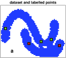
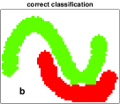
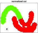
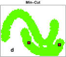
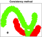
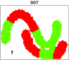
Figure 1: a. The unlabelled data in blue; labelled points are marked in green and in red. Each of the $1360$ pixels correspond to a data point; the labeled pixels were enlarged for clarity. b. The correct classification. c. Clustering results of the unsupervised normalized cut algorithm (ShiMalik, ). d. The min-cut solution. e. The results of the semi-supervised consistency method of (scholkopf, ). f. The outcome of the spectral graph transducer algorithm (sgt, ), which is a semi-supervised extension of the normalized cut algorithm.

Searching for the minimal energy solution is equivalent to seeking the most probable joint classification (MAP). A possible remedy to the difficulties in this approach may then be to consider the probability distribution of all possible classifications. Blum et al. provided a first step in this direction using a randomized min-cut algorithm. In this work we provide a different solution based on statistical physics.

Basically each solution in our method is weighed by its energy $E(classification)$, also known as the Boltzmann weight, and its probability is given by:

$$\Pr(classification;T)\propto e^{-E(classification)/T}\vspace{-1cm}$$ (1)

where the “temperature” $T$ serves as a free parameter, and the energy $E$ takes into account both unlabelled and labelled points. Classification is then performed by marginalizing (1), thus estimating the probability that a point $i$ belongs to a class $c$. This formalism is often referred to as a Markov random field (MRF), which has been applied in numerous works, including in the context of semi-supervised learning by (zhu03, ). However, they seek the MAP solution (which corresponds to $T=0$), while we estimate the distribution itself (at $T\geq 0$).

Using the framework of statistical physics has several advantages in the context of semi-supervised learning: First, classification has a simple probabilistic interpretation. It yields a fuzzy assignment of points to class types, which may also serve as a confidence level in the classification. Secondly, since exactly estimating the marginal probabilities is, in most cases, intractable, statistical physics has developed elegant Markov chain Monte-Carlo (MCMC) methods which are suitable for estimating semi-supervised systems. Due to the inherent complexity of semi-supervised problems, ‘standard’ MCMC methods, such as the Metropolis (Metropolis, ) and Swendsen-Wang (wang90, ) methods provide poor results, and one needs to apply more sophisticated algorithms, as discussed in section 3. Thirdly, using statistical physics allows us to gain an intuition regarding the nature of a semi-supervised problem, i.e., it allows for a detailed analysis of the effect of adding labelled points to an unlabelled data set. In addition, our method also has two practical advantages: (i) while most semi-supervised learning methods consider only the case of two class types, our method is naturally extended to the multi-class scenario. (ii) Another unique feature of our method is its ability to suggest the existence of a new class type, which did not appear in the labelled set.

Our main objective in this paper is to present a framework, which can later be applied in different directions. For example, the energy function in (1) can be any of the functions used in other semi-supervised methods. In this paper we chose to use the min-cut cost function. We do not claim that using this cost function is optimal, and indeed we observed that it is suboptimal in some cases. However, we aim to convince the reader that applying our method, to any energy function, would always yield equal or better results than merely minimizing the same energy function.

Our work is closely related to the typical cut criterion for unsupervised learning, first introduced by (blatt96, ) in the framework of statistical physics and later in a graph theoretic context by (GdalyahuEtAl99, ). The method introduced in this work can be viewed as an extension of these clustering algorithms to the semi-supervised case.

The paper is organized as follows: Section 2 presents the model, and Section 3 discusses the issue of estimating marginal probabilities. Section 4 presents the qualitative effect of adding labelled points. Our semi-supervised algorithm is outlined in Section 5. Section 6 demonstrates the performance of our algorithm on a toy data set and on two real-life examples of gene expression data.

2 Model definition

In our model each data point $i,i=1,\ldots,N$, corresponds to a random variable, or spin, $s_{i}$ which can take one of $q\geq 2$ discrete states. The number of states $q$ matches the number of class types in the labelled set. A certain classification of the data set then corresponds to a vector ${\bf S}$, ${\bf S}=\{s_{1},\ldots,s_{N}\}$. Assume that the first $M\ll N$ points are labelled, i.e., the state of spin $s_{k},1\leq k\leq M$ is clamped to a spin value $c_{k}$, which corresponds to the class type of point $k$. Hence the energy $E$ in our case is simply the Potts model energy of a granular ferromagnet with an external field;

$$E({\bf S})=\sum_{\langle i,j\rangle}J_{ij}(1-\delta_{s_{i},s_{j}})+\sum_{k=1}^{M}h_{k}(1-\delta_{s_{k},c_{k}}).$$ (2)

where $J_{ij}>0$ is a predefined similarity between points $i$ and $j$, $\langle i,j\rangle$ stands for all edge of neighboring graph, and $\delta_{s_{i},s_{j}}=1$ when $s_{i}=s_{j}$ and zero otherwise. The second term which corresponds to the labelled points, is known as the ‘external field’ term. In case the value of $s_{k}$ is different from the point’s assigned class $c_{k}$, the energy is increased by a value $h_{k}$. We used $h_{k}=\infty$, which assigns non-zero probability only to classifications in which $s_{k}=c_{k}$. Notice that one can introduce uncertain labels by using finite values of $h_{k}$, but we do not consider this case in this work.

The major problem in applying the suggested method concerns the difficulty in calculating (1). Since the number of possible classifications is exponential in $N$, one often needs to apply sampling MCMC algorithms, which are considered in the next section.

3 Estimating marginal probabilities

Introducing labelled points inherently changes the properties of the system and poses great difficulties in MCMC sampling. Labelled points may introduce ‘frustration’ into the system (a term borrowed from statistical physics); if, for example, point $i$ is connected to a couple of differently labelled points $j$ and $k$, it is ‘frustrated’ since whenever it matches one of them it contradicts the other. Such frustration appears also in physical systems of spin glasses, and is known to complicate their analysis.

The difficulty in sampling from spin glass systems results from their ragged energy landscape. The energy landscape can be described as being composed of several ‘valleys’ which are surrounded by very high energy barriers, which the sampling method is unable to traverse at low temperatures. As a results, ‘standard’ MCMC methods, e.g. the Metropolis and the Swendsen-Wang methods, are confined to a certain ‘valley’ for an exponential number of Markov chain steps, thus their estimates may be highly biased.

Extended MCMC methods is a title given for a family of methods which enable efficient sampling in complex scenarios such as spin-glasses (iba01, ). Extended MCMC methods solve the sampling problem by allowing the system to ‘jump’ between ‘valleys’. This is implicitly performed by letting the system pass through high energy configurations, which most likely erase any memory of the originating ‘valley’. In this work we applied the Multicanonical Monte-Carlo method (berg92a, ), which is a member of the extended MCMC methods.

The Multicanonical Monte-Carlo method first estimates the density of states $D(E)$, i.e. the number of different classifications at a given energy. It then generates a sample of classifications, $\{{\bf S}\}$, drawn from the distribution $Pr_{D}({\bf S})\propto 1/D(E({\bf S}))$, which can then be used to recover the Boltzmann distribution (1), for all temperatures $T$ at once. Sampling from $Pr_{D}({\bf S})$ yields a uniform distribution over all energy levels, which forces the MCMC to pass through high energy configurations and by that overcome the energy barriers. For further details about the method we refer the reader to (iba01, ).

Before presenting the effect of labelled points, we would like to shortly discuss an alternative to MCMC sampling, which is to approximate the marginal probabilities using methods from the field of graphical models. The intimate connections between statistical physics and graphical models have been demonstrated, e.g. by (YedidiaEtAlIJCAI01, ). Our Boltzmann distribution corresponds to an undirected graphical model, thus estimating the marginal probabilities is equivalent to performing inference in this model. Since exact inference, via the junction tree algorithm (Pearl88, ), is generally intractable, one needs to resort to approximate methods, such as (loopy) belief propagation (BP) or generalized belief propagation (GBP) (YedidiaEtAlIJCAI01, ). In our experimental study the performance of BP was rather poor, probably since the graphical model of a typical semi-supervised problem contains many short loops. On the other hand the performance of GBP was excellent, when applied to two dimensional problems, as in Fig. 1. However, to date there exists no principled way of applying GBP to a general graph, which guarantees good approximate inference, therefore we consider only MCMC sampling.

4 The effect of labelled points

As explained in section 3 the labelled points inherently complicate the sampling of the system. On the other hand, adding labelled points has the desired effect on classification. In order to understand this phenomenon we first describe the unsupervised case and then qualitatively explain the effects of adding labelled points.

The properties of a system, governed by the Boltzmann distribution (1), changes with the temperature $T$. In many physical systems, the temperature range $T\geq 0$ can be divided into intervals, or phases, each of which has its own global properties. Granular-ferromagnets without external fields (i.e. keeping the first term of (2)), which correspond to the unsupervised case, are known to have three phases (wiseman98, ); a low-temperature phase in which the system is ferromagnetic, i.e. most of the spins are assigned the same value; a high temperature phase in which the system is paramagnetic, i.e. the values assigned to the spins are nearly independent; and an intermediate phase termed the super-paramagnetic (SP) phase. In this phase, which is the most relevant for clustering, all spins of a grain (i.e. a cluster) are assigned a certain value, with different values at different grains. The clusters in the data can be identified in this SP phase; the larger the temperature interval of this phase, the more significant and stable is the clustering solution (levine, ).

Adding labelled points changes the system’s behavior. First, it effectively increases the strength of the interaction between spins near labelled points, which can be interpreted as an increase of their local density. As a result there is an increase in the transition temperature between the ordered SP phase and the unordered paramagnetic phase, thus increasing temperature interval of the SP phase at its the upper limit.

A second effect happens at low temperatures. For example, consider the case of two dense grains, each containing a labelled point of a different type, which are separated by a lower density region. In the SP phase the spins in each of the grains attain their correct class, but the spins in the low density region are still unordered. As the temperature is lowered the two classes ‘penetrate’ into the low density region until a ‘border’ between the classes is formed. Hence, from a semi-supervised perspective, the labelled points cause the low density region to be classified. Notice that at this temperature the unsupervised case is already at the ferromagnetic phase, where the two clusters are united. Hence, the labelled points also decrease the lower limit of the SP phase, which together with increasing its upper limit, results in a larger temperature interval relevant for classification.

When the temperature is further lowered, a different classification may appear. For example, one of the class types may overtake the whole system, similar to the min-cut solution in Fig. 1d, but, of course, we are not interested is such a solution.

Fig. 2 presents the effect of adding labelled points in the case of Fig. 1a. We plot the number of misclassified points using the algorithm in Sec. 5, as a function of $T$, in the unsupervised (US) and in the semi-supervised (SS) cases. In this data set we calculated (1) exactly using the junction tree algorithm (exact US and exact SS), and compared it to Multicanonical sampling (MC). Notice that adding labelled points decreases the number of errors dramatically, achieving almost correct classification over a large temperature interval ($0.5\leq T\leq 1$). At lower temperatures, which correspond to the min-cut solution (Fig. 1d), the number of misclassified points is large.

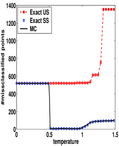
Figure 2: Classification error as a function of $T$ for the data set in Fig.1a. A comparison between the unsupervised case (exact US) and the semi-supervised case (exact SS), calculated exactly using the junction tree algorithm, and the Multicanonical MCMC method (MC).

5 The algorithm

Our semi-supervised learning algorithm is comprised of two parts: an estimation part, and a classification part which are described below.  

Estimation

consists of three stages:
$\bullet$ Map each point $i$ to a $q$-state random variable $s_{i}$, where $q$ is the number of class types of labelled points.
$\bullet$ Construct a graph $G$ of neighboring points $i$ and $j$ and assign a their pairwise similarity $J_{ij}>0$.
$\bullet$ Estimate the marginal probabilities $p_{i}(s_{i};T)$ and $p_{ij}(s_{i},s_{j};T)$, as explained in Sec. 3.

Classification

of a point $i$ at a temperature $T$ can simply be performed by $\mbox{argmax}_{1\leq k\leq q}p_{i}(s_{i}=k;T)$. However, we suggest a heuristic method which is slightly more elaborate, but takes into account the confidence in the classification, and also allows to identify new class types. This heuristic is comprised of two steps:
$\bullet$ Classify ‘confident’ points, using single point probabilities $p_{i}$: For each point $i$ we find the two most probable class assignments and their probabilities; $p_{1}$ and $p_{2}$. In case $p_{1}-p_{2}>\tau$, where $\tau>0$ is a user defined confidence parameter, we classify point $i$ according to the type which corresponds to $p_{1}$.
$\bullet$ Classify the remaining, less ‘confident’ points, using the pairwise probabilities $p_{ij}$: Following the intuition of (blatt96, ) we estimate the pairwise correlations between $i$ and $j$ defined as

$$C_{ij}(T)=\sum_{k=1}^{q}p_{ij}(s_{i}=k,s_{j}=k;T),\vspace{-0.15cm}$$

where the correlation ranges from the random level $1/q$, to a perfect correlation value of $1$. We then delete edges from the graph G for which $C_{ij}(T)<\frac{1}{2}\left(1+\frac{1}{q}\right)$, i.e., half way between random level and perfect correlation, and find the connected components of the resulting graph. Each ‘unconfident’ point $j$ is then classified according to the connected component to which it belongs. In case $j$ belongs to a connected component which contains points (already) classified as $c_{k}$, then $j$ is assigned to $c_{k}$. If $j$ belongs to a connected component which contains points which were assigned to several different classes, it is remains unassigned and is marked as “confused” between these classes. Finally, all the points which belong to a connected component that does not contain any classified point are marked as a new class.  

Notice that the classification depends on $T$. The rational is to supply the user with a classification ‘profile’ of each data point, over all temperatures. Since statistically significant classifications span large temperature intervals, such a ‘profile’ is rather limited in size. For example, the ‘profile’ of a point $j$ which resides in class $c_{1}$, close to the border with class $c_{2}$ would contain two classifications: at low temperatures $j$ is assigned to $c_{1}$, and at higher temperatures it is marked as “confused” between $c_{1}$ and $c_{2}$.
As for the value of $\tau$, our experimental study has shown that classification performance decreases with increasing the value of $\tau$ (data not shown), thus we chose to use $\tau=0.1$.

In case there are no labelled points $p_{i}(s_{i}=k)=1/q~{}\forall i,k$ then all points are treated as ‘unconfident’, and our ‘classification’ simply coincides with the clustering procedure of (blatt96, ).

6 Experimental results

We present results over three data sets: A toy data set, and two real-life data sets of gene expression.

6.1 Toy data

Fig. 3 presents a toy data set similar to Fig. 1, which contains $1306$ data points from three classes. As in the former toy data, the similarity between adjacent pixels is of unit value, hence the three classes form one connected cluster, which can not be separated without the labelled points.

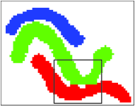
Figure 3: A toy data set comprised of three classes. Each pixel corresponds to a data point, and $J_{ij}=1$ for all adjacent pixels $i$ and $j$. The labelled points are randomly sampled with a uniform distribution. In order to enable correct classification the labelled points from the lower two classes are sampled from the area marked by a rectangle.

In order to evaluate the performance of our approach we carried two sets of experiments. In the first set we randomly chose $M$ labelled points ($M=5,10,15$ and $20$) from the two lower (green and red) classes, i.e. $q=2$, while in the second set of experiments the labelled points where randomly chosen from all three classes, i.e. $q=3$. For each value of $M$ and $q$ we evaluated $100$ instances (realizations) of random labelling, and the number of misclassified points appear in Fig. 4. The number of misclassified points in the unsupervised case was $1001$, and was evaluated as explained in Sec. 5.

As expected, incorporating even a few labelled points has a significant impact on the number of misclassified points. As can be seen, the results highly depend on the specific instance of labelled points, hence the average performance is less informative. Therefore the instances are presented in an increasing order of misclassified points of our approach (MC), while the other two lines correspond to the graph-cuts method (GC) and to the local-global consistency method (scholkopf, ) (LGC). In order to plot the MC line in Fig. 4 we automatically selected a temperature, $T^{*}$, in which classification is significantly different from the ground state ($T=0$) solution, and is also most ‘stable’. At each $T$ we consider only the points, $c(T)$, whose classification is both confident and different than the $T=0$ solution. We define a score $\eta(T)=\|c(T)\|\cdot s(T)$, where $s(T)$ is the average temperature interval in which the classifications of $c(T)$ remain unchanged. Then, $T^{*}=\arg\max\eta(T)$, and in case $\eta(T^{*})<\eta_{0}$, we set $T^{*}=0$. In general, we recommend to use the ‘profiles’ of the points, since there may be several ‘stable’ solutions at different temperatures.

In comparing our method and graph-cuts, both of which use the same energy function, it can be observed that our method always achieves an equal or lower number of misclassifications than graph-cuts. However, it appears that in several instances of labelled points, it is preferable to apply the energy function of (scholkopf, ).
Also it seems that for $q=2$ our method significantly outperforms the other two methods, mainly due to its ability to identify the third class type, although none of its points is labelled. For $q=3$ the solutions of graph-cuts and of our method become similar as the number of labelled points increases.

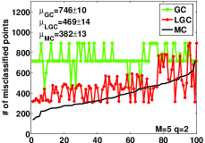
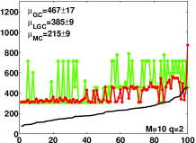
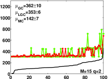
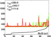
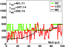
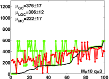
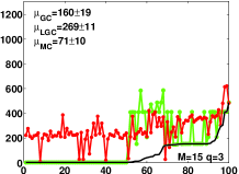
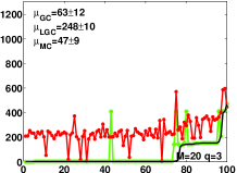
Figure 4: The number of misclassification out of $1306$ points of Fig. 3, for $q=2$ (upper row) and for $q=3$ (lower row) for $100$ random samples of labelled points $M$ ($M=5,10,15$ and $20$ from left to right). We compare our method (MC, black line) to graph-cuts (GC, red line) and to the local-global method (LGC, green line). Also shown is the mean performance $\mu$ and its standard deviation. In the unsupervised case the number of misclassified points was $1001$.

6.2 Leukemia gene expression data set

In this section we present the results of applying our algorithm to a real-world problem of cancer classification and class discovery. In cancer research, there is a particular need for semi-supervised techniques, as the classes and sub-classes (cancer types) are only partially known. Hence one needs to apply methods that can help partition the data into known classes and possibly identify novel ones.

Our example is based on gene expression data of acute leukemia published by (armstrong02, ). They analyzed three different types of acute leukemia; acute myeloid leukemia (AML), acute lymphoblastic leukemia (ALL) and a sub-type of ALL which carries a chromosomal translocation in the MLL gene. Armstrong et al.  show (in a supervised manner) that this sub-type has a distinct molecular profile and can be considered a new type of leukemia termed MLL.

We applied our algorithm to the 57 leukemia samples in (armstrong02, ) ($20$ ALL, $20$ AML and $17$ MLL samples), each described by the expression levels of the 200 genes with largest variance across samples. The similarity between samples was calculated in a standard manner in this field. The same as in Sec. 6.1, we carried two set of experiments. In the first set of experiments we randomly chose $M$ points ($M=2,4,6$) from the ALL and AML samples but not from the MLL class, and in the second set of experiments $M$ labelled points ($M=3,6,9$) were randomly selected from all three classes. The results appear in Fig. 5 in the same format as in Fig. 4. The number of misclassified points in the unsupervised case was $11$.

As in the previous data set, our method always achieves an equal or lower number of misclassifications than graph-cuts. Notice that in the $q=2$ case, our method is able to predict the existence of MLL, while all $17$ MLL points are misclassified in the other methods. It appears that for this data set, applying the min-cut cost function is almost always superior to the quadratic cost function of (scholkopf, ). Another interesting phenomenon is the relatively low number of misclassifications in the unsupervised case. It happens that in $20\%-40\%$ of the instances (depending on $q$ and $M$) it is preferable to apply our method without the labelled points.

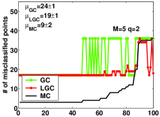
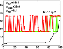
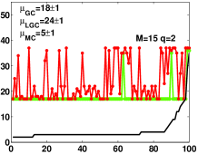
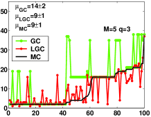
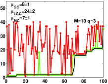
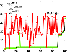
Figure 5: The same as in Fig. 4 but for $57$ leukemia samples. The values of $q$ and $M$ appears in each panel. The number of misclassified points in the unsupervised case was $11$.

6.3 Yeast cell cycle gene expression data

In this section we describe an application of our method to a real-life problem in cellular biology for which the true solution is partly unknown. This concerns the assignment of the yeast’s genes to the stage in the cell cycle in which they are expressed. While the yeast’s genome is well-characterized, the function of many of its genes remains to be determined. Therefore, correctly assigning genes to their cell cycle phase may shed light on their function and help connect them to the emerging cellular network.

The Yeast’s cell cycle was studied by various researchers, typically by applying unsupervised methods, e.g. (spellman, ; alter, ). Here we use the data of Spellman et al. which measured the expression level of the yeast’s genes at $18$ specific times over the course of two cell-cycles, thus data consists of $18$ measurements of more than $6000$ genes. Due to experimental difficulties some of the entries in this $18\times 6000$ matrix are missing, hence following (alter, ) we used a subset of $4523$ genes for which at least $15$ out of the $18$ readings are available. For $77$ of these genes, the assignment to one of $5$ stages in the cell cycle (M/G1, G1, S, S/G2 and G2/M) is well established. Therefore, we have a multi-class classification problem ($q=5$) of $4523$ points in $18$ dimensions, with $77$ labelled points. As a similarity measure we used a standard protocol as in Sec. 6.2.

Since ground truth is not available in this problem we decided to measure the success rate of our method by comparing our results to the proposed classification of Spellman et al. They used several biological criteria in order to rank the genes according to their participation in the cell-cycle. Their list consists of $604$ out of the $4523$ genes, and $69$ of them also appear in the list of known $77$ genes, leaving $535$ genes as a test set.

We classified the $535$ points to one of the $5$ classes, or marked them as ‘confused’ between classes. When considering only the classified points and treating the ‘confused’ points as errors our average success rate is 32% (over the 5 classes), while graph-cuts reaches 20%.

7 Discussion

We introduced an approach to semi-supervised learning which is based on statistical physics. Our approach may be applied to any energy function, and yields an equal or better performance than minimizing the same energy function. Our method is most suitable in case the number labelled points is small, since its classifications would coincide with the minimal energy solution as the number of labelled points becomes larger.

The method is based on the Multicanonical MCMC method, which allows for an efficient estimation of the Boltzmann distribution, even in the multi-class scenario. The basic difficulty in methods which seek the minimal energy, i.e. work at $T=0$, is that the multi-class scenario is NP-hard. We avoid such difficulties since the interesting regime for classification is $T>0$.

The computational complexity of MCMC is hard to estimate, as it is problem dependent. A large multi-class data set may indeed be difficult to sample, and require a long run, which calls for even more efficient MCMC or approximation methods. However, we hope to have convinced the reader that our performance gain over other, more efficient, methods may be worthwhile.

Although our results display the advantages of incorporating labelled points in an unsupervised setting, the performance highly depends on the specific choice of labelled points, and in some cases it is even preferable to ignore the labelled points. A related phenomenon already appeared in previous work, e.g. (iraCohen, ), and should be thoroughly addressed.

References

- (1) O. Alter et al. Generalized singular value decomposition for comparative analysis of genome-scale expression data sets of two different organisms. Proc. Natl. Acad. USA, 100:3351–3356, 2003.
- (2) S.A. Armstrong et al. MLL translocations specify a distinct gene expression profile that distinguishes a unique leukemia. Nature Gen., 30:41–47, 2002.
- (3) B.A. Berg and T. Neuhaus. Multicanonical ensemble: A new approach to simulate first-order phase transitions. Phys. Rev. Lett., 68:9–12, 1992.
- (4) M. Blatt, S. Wiseman, and E. Domany. Data clustering using a model granular magnet. Neural Computation, 9:1805–1842, 1997.
- (5) A. Blum and S. Chawla. Learning from labeled and unlabeled data using graph mincuts. In ICML, 2001.
- (6) A. Blum, J. Lafferty, M. R. Rwebangira, and R. Reddy. Semi-supervised learning using randomized mincuts. In ICML, 2004.
- (7) Y. Boykov, O. Veksler, and R. Zabih. Fast approximate energy minimization via graph cuts. In ICCV, 1999.
- (8) I. Cohen, F.G. Cozman, N. Sebe, M.C. Cirelo, and T.S Huang. Semi-supervised learning of classifiers: Theory, algorithms for bayesian network classifiers and application to human-computer interaction. PAMI, pages 1553–1567, 2004.
- (9) Y. Gdalyahu, D. Weinshall, and M. Werman. Stochastic image segmentation by typical cuts. In CVPR, 1999.
- (10) Y. Iba. Extended ensemble monte carlo. International Journal of Modern Physics C, 12:623–656, 2001.
- (11) T. Joachims. Transductive learning via spectral graph partitioning. In ICML, 2003.
- (12) E. Levine and E. Domany. Unsupervised estimation of cluster validity using resampling. Neural Computation, pages 2573–2593, 2001.
- (13) N. Metropolis et al. Equations of state calculations by fast computing machines. ournal of Chemical Physics, 21:1087–1092, 1953.
- (14) J. Pearl. Probabilistic reasoning in intelligent systems: Networks of plausible inference. 1988.
- (15) J. Shi and J. Malik. Normalized cuts and image segmentation. PAMI, 22(8):888–905, 2000.
- (16) P.T. Spellman et al. Comprehensive identification of cell cycle-regulated genes of the yeast saccharomyces cerevisiae by microarray hybridization. Molecular Biology of the Cell, 9:3273–3297, 1998.
- (17) J.S. Wang and R.H Swendsen. Cluster Monte Carlo algorithms. Physica A, 167:565–579, 1990.
- (18) S. Wiseman, M. Blatt, and E. Domany. Super-paramagnetic clustering of data. Phys. Rev. E, 57:3767–3783, 1998.
- (19) J.S. Yedidia, W.T. Freeman, and Y. Weiss. Generalized belief propagation. In NIPS, 2000.
- (20) S.X. Yu and J. Shi. Grouping with bias. In NIPS, 2001.
- (21) D. Zhou, O. Bousquet, T.N. Lal, J. Weston, and B. Scholkopf. Learning with local and global consistency. In NIPS, 2003.
- (22) X. Zhu, Z. Ghahramani, and J. Laferty. Semi-supervised learning using Gaussian fields and harmonic functions. In ICML, 2003.