Minimum-Cost Coverage of Point Sets by Disks

Abstract

We consider a class of geometric facility location problems in which the goal is to determine a set $X$ of disks given by their centers ($t_{j}$) and radii ($r_{j}$) that cover a given set of demand points $Y\subset{}^{2}$ at the smallest possible cost. We consider cost functions of the form $\sum_{j}f(r_{j})$, where $f(r)=r^{\alpha}$ is the cost of transmission to radius $r$. Special cases arise for $\alpha=1$ (sum of radii) and $\alpha=2$ (total area); power consumption models in wireless network design often use an exponent $\alpha>2$. Different scenarios arise according to possible restrictions on the transmission centers $t_{j}$, which may be constrained to belong to a given discrete set or to lie on a line, etc.

We obtain several new results, including (a) exact and approximation algorithms for selecting transmission points $t_{j}$ on a given line in order to cover demand points $Y\subset{}^{2}$; (b) approximation algorithms (and an algebraic intractability result) for selecting an optimal line on which to place transmission points to cover $Y$; (c) a proof of NP-hardness for a discrete set of transmission points in ² and any fixed $\alpha>1$; and (d) a polynomial-time approximation scheme for the problem of computing a minimum cost covering tour (MCCT), in which the total cost is a linear combination of the transmission cost for the set of disks and the length of a tour/path that connects the centers of the disks.

; F.2.2 [Nonnumerical Algorithms and Problems]: Geometrical problems and computations

General Terms: Algorithms, Theory.

Keywords: Covering problems, tour problems, geometric optimization, complexity, approximation.

1 Introduction

The problem.  We study a geometric optimization problem that arises in wireless network design, as well as in robotics and various facility location problems. The task is to select a number of locations $t_{j}$ for the base station antennas (servers), and assign a transmission range $r_{j}$ to each $t_{j}$, in order that each $p_{i}\in Y$ for a given set $Y=\{p_{1},\ldots,p_{n}\}$ of $n$ demand points (clients) is covered. We say that client $p_{i}$ is covered if and only if $p_{i}$ is within range of some transmission point $t_{j_{i}}$, i.e., $d(t_{j_{i}},p_{i})\leqslant r_{j_{i}}$. The resulting cost per server is some known function $f$, such as $f(r)=r^{\alpha}$. The goal is to minimize the total cost, $\sum_{j}f(r_{j})$, over all placements of at most $k$ servers that cover the set $Y$ of clients.

In the context of modeling the energy required for wireless transmission, it is common to assume a superlinear ($\alpha>1$) dependence of the cost on the radius; in fact, physically accurate simulation often requires superquadratic dependence ($\alpha>2$). A quadratic dependence ($\alpha=2$) models the total area of the served region, an objective arising in some applications. A linear dependence ($\alpha=1$) is sometimes assumed, as in Lev-Tov and Peleg[19], who study the base station coverage problem, minimizing the sum of radii. The linear case is important to study not only in order to simplify the problem and gain insight into the general problem, but also to address those settings in which the linear cost model naturally arises[10, 21]. For example, the model may be appropriate for a system with a narrow-angle beam whose direction can either rotate continuously or adapt to the needs of the network. Another motivation for us comes from robotics, in which a robot is to map or scan an environment with a laser scanner[14, 13]: For a fixed spatial resolution of the desired map, the time it takes to scan a circle corresponds to the number of points on the perimeter, i.e., is proportional to the radius.

Our problem is a type of clustering problem, recently named min-size $k$-clustering by Bilò et al.[7]. Clustering problems tend to be NP-hard, so most efforts, including ours, are aimed at devising an approximation algorithm or a polynomial-time approximation scheme (PTAS).

We also introduce a new problem, which we call minimum cost covering tour (MCCT), in which we combine the problem of finding a short tour and placing covering disks centered along it. The objective is to minimize a linear combination of the tour length and the transmission/covering costs. The problem arises in the autonomous robot scanning problem[14, 13], where the covering cost is linear in the radii of the disks, and the overall objective is to minimize the total time of acquisition (a linear combination of distance travelled and sum of scan radii). Another motivation is the distribution of a valuable or sensitive resource: There is a trade-off between the cost of broadcasting from a central location (thus wasting transmission or risking interception) and the cost of travelling to broadcast more locally, thereby reducing broadcast costs but incurring travel costs.

Location Constraints.  In the absence of constraints on the server locations, it may be optimal to place one server at each demand point. Thus, we generally set an upper bound, $k$, on the number of servers, or we restrict the possible locations of the servers. Here, we consider two cases of location constraints:

(1) Servers are restricted to lie in a discrete set $\{t_{1},\ldots,t_{m}\}$; or

(2) Servers are constrained to lie on a line (which may be fully specified, or may be selected by the optimization).

Our results.  We provide a number of new results, some improving previous work, some giving the first results of their kind.

In the discrete case studied by Lev-Tov and Peleg[19], and Biló et al.[7], we give improved results. For the discrete 1D problem where $Y\subseteq\mathbb{R}$, we improve their 4-approximation to a linear-time 3-approximation by using a “Closest Center with Growth” (CCG) algorithm, and, as an alternative to the previous $O((n+m)^{3})$ algorithm[19], we give a near-linear-time 2-approximation that uses a “Greedy Growth” (GG) algorithm. Unfortunately, we cannot extend our proofs to the 1$\frac{1}{2}$D problem. Intuitively, greedy growth works as follows: start with a disk with center at each server, each disk of radius zero; among all clients, find one that requires the least radial disk growth to capture it; repeat until all clients are covered. Note that for $\alpha\geqslant 2$ the 2D variants of the problem are already proved to be NP-Hard and to have a PTAS[7].

In the general 2D case with clients $Y\subset{}^{2}$, we strengthen the hardness result of Biló et al. [7] by showing that the discrete problem is already hard for any superlinear cost function, i.e., $f(r)=r^{\alpha}$ with $\alpha>1$. Furthermore, we generalize the min-size clustering problem in two new directions. On the one hand, we consider less restrictive server placement policies. For instance, if we only restrict the servers to lie on a given fixed line, we give a dynamic programming algorithm that solves the problem exactly, in time $O(n^{2}\log n)$ for any $L_{p}$ metric in the linear cost case, and in time $O(n^{4}\log n)$ in the case of superlinear non-decreasing cost functions. For simple approximations, our algorithm “Square Greedy” (SG) gives in time $O(n\log n)$ a $3$-approximation to the square covering problem with any linear or superlinear cost function. A small variation, “Square Greedy with Growth” (SGG), gives a 2-approximation for a linear cost function, also in time $O(n\log n)$. The results are also valid for covering by $L_{p}$ disks for any $p$, but with correspondingly coarser approximation factors.

A practical example in which servers are restricted to lie along a line is that of a highway that cuts through a piece of land, and the server locations are restricted to lie along the highway. The line location problem arises when one not only needs to locate the servers, but also needs to select an optimal corridor for the placement of the highway. Other relevant examples may include devices powered by a microwave or laser beam lining up along the beam.

If the servers are restricted to lie on a horizontal line, but the location of this line may be chosen freely, then we show that the exact optimal position (with $\alpha=1$) is not computable by radicals, using an approach similar to that of Bajaj[5, 6] in addressing the unsolvability of the Fermat-Weber problem. On the positive side, we give a fully polynomial-time approximation scheme (FPTAS) requiring time $O((n^{3}/\varepsilon)\log n)$ if $\alpha=1$ and time $O((n^{5}/\varepsilon)\log n)$ if $\alpha>1$.

For servers on an unrestricted line, of any slope, and $\alpha=1$, we give $O(1)$-approximations (4-approximation in $O(n^{4}\log n)$ time, or $8\sqrt{2}$-approximation in $O(n^{3}\log n)$ time) and an FPTAS requiring time $O((n^{5}/\varepsilon^{2})\log n)$.

We give the first algorithmic results for the new problem, minimum cost covering tour (MCCT), which we introduce. Given a set $Y\subseteq\mathbb{R}^{2}$ of $n$ clients, our goal is to determine a polygonal tour $T$ and a set $X$ of $k$ disks of radii $r_{j}$ centered on $T$ that cover $Y$ while minimizing the cost $\mathrm{length}(T)+C\sum r_{i}^{\alpha}$. Our results are for $\alpha=1$. The ratio $C$ represents the relative cost of touring versus transmitting. We show that MCCT is NP-hard if $C$ is part of the input. At one extreme, if $C$ is small then the optimum solution is a single server placed at the circumcenter of $Y$ (we can show this to be the case for $C\leqslant 4$). At the other extreme (if $C$ very large), the optimum solution is a TSP among the clients. For any fixed value of $C>4$, we present a PTAS for MCCT, based on a novel extension of the $m$-guillotine methods of [20].

Related work.  There is a vast family of clustering problems, among which are the $k$-center problem in which one minimizes $\max_{j}r_{j}$, the $k$-median problem in which one minimizes $\sum_{i}d(p_{i},t_{j_{i}})$, and the $k$-clustering problem in which one minimizes the maximum over all clusters of the sum of pairwise distances between points in that cluster. For the geometric instances of these related clustering problems, refer to the survey by Agarwal and Sharir[1]. When $k$ is fixed, the optimal solution can be found in time $O(n^{k})$ using brute force. In the plane, one of the only results for the min-size clustering problem is a small improvement for $k=2$ by Hershberger[17], in subquadratic time $O(n^{2}/\log\log n)$. Approximation algorithms and schemes have been proposed, particularly for geometric instances of these problems (e.g., [4]). Clustering for minimizing the sum of radii was studied for points in metric spaces by Charikar and Panigrahy[9], who present an $O(1)$-approximation algorithm using at most $k$ clusters.

For the linear-cost model ($\alpha=1$), our problem has been considered recently by Lev-Tov and Peleg[19] who give an $O((n+m)^{3})$ algorithm when the clients and servers all lie on a given line (the 1D problem), and a linear-time 4-approximation in that case. They also give a PTAS for the two-dimensional case when the clients and servers can lie anywhere in the plane. Bilò et al.[7] show that the problem is NP-hard in the plane for the case $f(r)=r^{\alpha}$, $\alpha\geqslant 2$, either when the sets $X$ and $Y$ are given and $k$ is left unspecified ($k=n$), or when $k$ is fixed but then $X=Y$. They give a PTAS for the linear cost case ($\alpha=1$) and a slightly more involved PTAS for a more general problem in which the cost function is superlinear, there are fixed additive costs associated with each transmission server and there is a bound $k$ on the number of servers.

There are many problems dealing with covering a set of clients by disks of given radius. Hochbaum and Maass[18] give a PTAS for covering with a minimum number of disks of fixed radius, where the disk centers can be taken anywhere in the plane. They introduce a “grid-shifting technique,” which is used and extended by Erlebach et al.[12]. Lev-Tov and Peleg[19] and Bilò et al.[7] extend the method further in obtaining their PTAS results for the discrete version of our problem.

When a discrete set $X$ of potential server locations is given, Gonzalez[16] addresses the problem of maximizing the number of covered clients while minimizing the number of servers supplying them, and he gives a PTAS for such problems with constraints such as bounded distance between any two chosen servers. In[8], a polynomial-time constant approximation is obtained for choosing a subset of minimum size that covers a set of points among a set of candidate disks (the radii can be different but the candidate disks must be given).

The closest work to our combined tour/transmission cost (MCCT) is the work on covering tours: the “lawn mower” problem[2], and the TSP with neighborhoods[3, 11], each of which has been shown to be NP-hard and has been solved with various approximation algorithms. In contrast to the MCCT we study, the radius of the “mower” or the radius of the neighborhoods to be visited is specified in advance.

2 Scenario (1): Server Locations Restricted to a Discrete Set

2.1 The one-dimensional discrete problem with linear cost

Consider the case of $m$ fixed server locations $X=\{t_{1},...,t_{m}\}$, $n$ client locations $Y=\{p_{1},...,p_{n}\}$, and a linear ($\alpha=1$) cost function, with clients and servers all located along a fixed line. Without loss of generality, we may assume that $X$ and $Y$ are sorted in the same direction, at an extra cost of $O((n+m)\log(n+m))$. Lev-Tov and Peleg[19] give an $O((n+m)^{3})$ dynamic programming algorithm for finding an exact solution. Bilò et al.[7] show that the problem is solvable in polynomial time for any value of $\alpha$ by reducing it to an integer linear program with a totally unimodular constraint matrix. The complexities of these algorithms, while polynomial, is high. Lev-Tov and Peleg also give a simple “closest center” algorithm (CC) that gives a linear-time $4$-approximation. We improve to a $3$-approximation in linear time, and a 2-approximation in $O(m+n\log m)$ time.

We now describe an algorithm which also runs in linear time, but achieves an approximation factor of $3$.

Closest Center with Growth (CCG) Algorithm: Process the clients $\{p_{1},...,p_{n}\}$ from left to right keeping track of the rightmost extending disk. Let $\omega_{R}$ denote the rightmost point of the rightmost extending disk, and let $R$ denote the radius of this disk. (In fact the rightmost extending disk will always be the last disk placed.) If $\omega_{R}$ is equal to, or to the right of the next client processed, $p_{i}$, then $p_{i}$ is already covered so ignore it and proceed to the next client. If $p_{i}$ is not yet covered, consider the distance of $p_{i}$ to $\omega_{R}$ compared with the distance of $p_{i}$ to its closest center $\hat{t_{i}}$. If the distance of $p_{i}$ to $\omega_{R}$ is less than or equal to the distance of $p_{i}$ to its closest center $\hat{t_{i}}$, then grow the rightmost extending disk just enough to capture $p_{i}$. Otherwise use the disk centered at $\hat{t_{i}}$ of radius $|p_{i}-\hat{t_{i}}|$ to cover $p_{i}$.

Lemma 1

For $\alpha=1$, CCG yields a $3$-approximation to OPT in $O(n+m)$ time.

The proof is similar to that of the next lemma, and omitted in this version.

If we consider a single disk $D$ with clients $p_{L}$ and $p_{R}$ on the left and right edges of $D$, associated centers $\hat{x}_{L}$, $\hat{x}_{R}$ at distances respectively radius($D$)$-\epsilon$ to the left and radius($D$)$-\epsilon$ to the right, along with a dense set of clients in the left hand half of $D$ we see that $3$ is the best possible constant for CCG.

Finally we offer an algorithm that achieves a $2$-approximation but runs in time $O(m+n\log{m})$.

Greedy Growth (GG) Algorithm: Start with a disk with center at each server all of radius zero. Now, amongst all clients, find the one which requires the least radial disk growth to capture it. Repeat until all clients are covered. An efficient implementation uses a priority queue to determine the client that should be captured next. One can set up the priority queue in $O(m)$ time. Note that the priority queue will never have more than $2m$ elements, and that each $p_{i}$ eventually gets captured, either from the right or from the left. Each capture can be done in time $O(\log{m})$ for a total running time of $O(m+n\log{m})$.

Lemma 2

For $\alpha=1$, GG yields a $2$-approximation to OPT in $O(m+n\log{m})$ time.

Proof 2.1.

Define intervals $J_{i}$ as follows: when capturing a client $p_{i}$ from a server $t_{j}$ whose current radius (prior to capture) is $r_{j}$, let $J_{i}=(t_{j}+r_{j},p_{i}]$ if $p_{i}>t_{j}$, and $J_{i}=[p_{i},t_{j}-r_{j})$ otherwise. Our first trivial yet crucial observation is that $J_{i}\cap J_{k}=\emptyset$ if $i\neq k$. Also note that the sum of the lengths of the $J_{i}$ is equal to the sum of the radii in the GG cover.

Consider now a fixed disk $D$ in OPT, centered at $t_{D}$, and the list of intervals $J_{i}$ whose $p_{i}$ is inside $D$. As before, at most one such $J_{i}$ extends outward to the right from the right edge of $D$. If so, call it $J_{R}$, and define $J_{L}$ symmetrically. If $J_{R}$ exists, it cannot extend more than radius($D$) to the right of $D$. Let $\lambda=\mathrm{length}(J_{R})$. We argue that there is an interval of length $\lambda$ in $D$, to the right of $t_{D}$, which is free of $J_{i}$’s. It follows that there is at most radius($D$) worth of segments to the right of $t_{D}$. Of course, this is also true if $J_{R}$ does not exist. By symmetry, there is also radius($D$) worth of segments to the left of $t_{D}$, whether $J_{L}$ exists or not, yielding the claimed $2$-approximation.

Assume $J_{R}$ exists. Then the algorithm successively extends $J_{R}$ by growth to the left up to some maximum point (possibly stopping right at $p_{R}$). Since the growth could have been induced by clients to the right of $J_{R}$, that maximum point is not necessarily a client. There is, however, some client inside $D$ that is captured last in this process. This client $p_{i}$ (possibly $p_{R}$) cannot be within $\lambda$ of $t_{D}$, since otherwise it would have been captured prior to the construction of $J_{R}$.

If there is no client between $t_{D}$ and $p_{i}$ we are done, since then there could be no interval $J_{k}$ in between. Thus consider the client $p_{i-1}$ just to the left of $p_{i}$. Suppose $d(p_{i-1},p_{i})\geqslant\lambda$. Then, if $p_{i-1}$ is eventually captured from the left, we would have the region between $p_{i-1}$ and $p_{i}$ free of $J_{k}$’s and be done. On the other hand, if $p_{i-1}$ is captured from the right, it must be captured by a server between $p_{i-1}$ and $p_{i}$, and that server is at least $\lambda$ to the left of $p_{i}$ since otherwise $p_{i}$ would be captured by that server prior to $p_{R}$. This leaves the distance from the server to $p_{i}$ free of $J_{k}$’s.

Hence the only case of concern is if $d(p_{i-1},p_{i})<\lambda$. Clearly $p_{i-1}$ must not have been captured at the time when $p_{R}$ is captured since otherwise $p_{i}$ would have been captured before $p_{R}$, contradicting the assumption that $p_{i}$ is captured by growth leftward from $p_{R}$. Similarly, there cannot be a server between $p_{i-1}$ and $p_{i}$, since otherwise both $p_{i-1}$ and $p_{i}$ would be captured before $p_{R}$. Together with the definition of $p_{i}$, this implies that $p_{i-1}$ is captured from the left. Therefore, to the left of $p_{i-1}$, there must be one or more intervals $\{J_{l_{i}}\}$ whose length is at least $\lambda$ that are constructed before $p_{i-1}$ is captured. Similarly, to the right of $p_{i}$, there must be some one or more intervals $\{J_{r_{j}}\}$ whose length is at least $\lambda$, constructed before $p_{i}$ is captured. However, either the last $J_{l_{i}}$ is placed before the last $J_{r_{j}}$ or vice versa. In the first case, there are no $\lambda$ length obstructions left in the left-hand subproblem, so $p_{i-1}$ will be covered, and with $\lambda$ length obstructions remaining in the right subproblem, $p_{i}$ will be captured by growth rightward. The second case is symmetrical to the first. In either case we have a contradiction.

To see that the factor $2$ is tight, just consider servers at $-2+\epsilon,0$ and $2-\epsilon$ and clients at $-1$ and $1$.

2.2 Hardness of the two-dimensional discrete problem with superlinear cost

In 2D, we sketch an NP-hardness proof, for any $\alpha>1$. This strengthens the NP-hardness proof of[7], which only works in the case $\alpha\geqslant 2$.

Theorem 2.1.

For any a fixed $\alpha>1$, let the cost function of a circle of radius $r$ be $f(r)=r^{\alpha}$. Then it is NP-hard to decide whether a discrete set of $n$ clients in the plane, and a discrete set of $m$ potential transmission points allow a cheap set of circles that covers all demand points.

Proof (sketch).  Let $I$ be an instance of Planar 3Sat, and let $G_{I}$ be the corresponding variable-clause incidence graph. After choosing a suitable layout of this planar graph, resulting in integer variables with coordinates bounded by a polynomial in the size of $G_{I}$ for all vertices and edges, we replace each the vertex representing any particular variable by a closed loop, using the basic idea shown in the left of Figure 1; this allows two fundamentally different ways of covering those points cheaply (using the “odd” or the “even” circles), representing the two truth assignments. For each edge from a vertex to a variable, we attach a similar chain of points that connects the variable loop to the clause gadget; the parity of covering a variable loop necessarily assigns a parity to all incident chains. Note that choosing sufficiently fine chains guarantees that no large circles can be used, as the overall weight of all circles in a cheap solution will be less than 1. (It is straightforward to see that for any fixed $\alpha>1$, this can be achieved by choosing coordinates that are polynomial in the size of $G_{I}$, with the exponent being $O(1/(\alpha-1))$.)

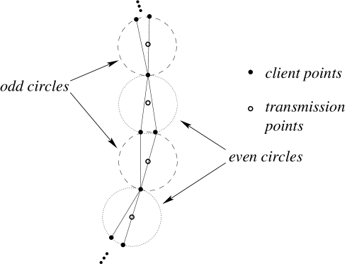
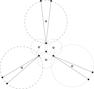
Figure 1: (Left) The switch structure of a variable gadget. Note how there are two fundamentally different ways to cover all points cheaply. (Right) The structure of a clause gadget. One small circle is needed for picking up the client point at the center of the gadget.

For the clauses choose a hexagonal arrangement as shown in the right of Figure 1: There is one central point that must be covered somehow; again, $\alpha>1$ guarantees that it is cheaper to do this from a nearby transmission point, rather than increasing the size of a circle belonging to a chain gadget.

Now it is straightforward to see that there is a cheap cover, using only the forced circles, iff the truth assignment corresponding to the covering of variabe loops assures that each clause has at least one satisfying variable. ∎

3 Scenario (2): Server Locations
Restricted to a Line

3.1 Servers along a fixed horizontal line

3.1.1 Exact solutions

Suppose that the servers are required to lie on a fixed horizontal line, which we take without loss of generality to be the $x$-axis. Such a restriction could arise naturally (e.g., the servers must be connected to a power line, must lie on a highway, or in the main corridor in a building). In addition, this case must be solved first before attempting to solve the more general problem—along a polygonal curve.

In this section, we describe dynamic programming algorithms to compute a set of server points of minimum total cost. For notational convenience, we assume that the clients $Y$ are indexed in left-to-right order. Without loss of generality, we also assume that all the clients lie on or above the $x$-axis, and that no two clients have the same $x$-coordinate. (If a client $p_{i}$ lies directly above another client $p_{j}$, then any circle enclosing $p_{i}$ also encloses $p_{j}$, so we can remove $p_{j}$ from $Y$ without changing the optimal cover.)

Let us call a circle $C$ pinned if it is the leftmost smallest axis-centered circle enclosing some fixed subset of clients. Equivalently, a circle is pinned if it is the leftmost smallest circle passing through a chosen client or a chosen pair of clients. Under any $L_{p}$ metric, there are at most $O(n^{2})$ pinned circles. As long as the cost function $f$ is non-decreasing, there is a minimum-cost cover consisting entirely of pinned circles.

Linear Cost.  If the cost function $f$ is linear (or sublinear), we easily observe that the circles in any optimum solution must have disjoint interiors. (If two axis-centered circles of radius $r_{i}$ and $r_{j}$ intersect, they lie in a larger axis-centered circle of radius at most $r_{i}+r_{j}$.) In this case, we can give a straightforward dynamic programming algorithm that computes the optimum solution under any $L_{p}$ metric.

The algorithm given in Figure 2 (left) finds the minimum-cost cover by disjoint pinned circles, where distance is measured using any $L_{p}$ metric. We call the rightmost point enclosed by any pinned circle $C$ the owner of $C$.

If we use brute force to compute the extreme points enclosed by each pinned circle and to test whether any points lie directly above a pinned circle, this algorithm runs in $O(n^{3})$ time. With some more work, however, we can improve the running time by nearly a linear factor.

This improvement is easiest in the $L_{\infty}$ metric, in which circles are axis-aligned squares. Each point $p_{i}$ is the owner of exactly $i$ pinned squares: the unique axis-centered square with $p_{i}$ in the upper right corner, and for each point $p_{j}$ to the left of $p_{i}$, the leftmost smallest axis-centered square with $p_{i}$ and $p_{j}$ on its boundary. We can easily compute all these squares, as well as the leftmost point enclosed by each one, in $O(i\log i)$ time. (To simplify the algorithm, we can actually ignore any pinned square whose owner does not lie on its right edge.) If we preprocess $P$ into a priority search tree in $O(n\log n)$ time, we can test in $O(\log n)$ time whether any client lies directly above a horizontal line. The overall running time is now $O(n^{2}\log n)$.

For any other $L_{p}$ metric, we can compute the extreme points enclosed by all $O(n^{2})$ pinned circles in $O(n^{2})$ time using the following duality transformation. If $C$ is a circle centered at $(x,0)$ with radius $r$, let $C^{*}$ be the point $(x,r)$. For each client $p_{i}$, let $p_{i}^{*}=\{C^{*}|\mbox{$C$ is centered on the $x$-axis and }p_{i}\in C\}$, and let $Y^{*}=\{p_{i}^{*}\mid p_{i}\in Y\}$. We easily verify that each set $p_{i}^{*}$ is an infinite $x$-monotone curve. (Specifically, in the Euclidean metric, the dual curves are hyperbolas with asymptotes of slope $\pm 1$.) Moreover, any two dual curves $p_{i}^{*}$ and $p_{j}^{*}$ intersect exactly once; i.e., $Y^{*}$ is a set of pseudo-lines. Thus, we can compute the arrangement of $Y^{*}$ in $O(n^{2})$ time. For each pinned circle $C$, the dual point $C^{*}$ is either one of the clients $p_{i}$ or a vertex of the arrangement of dual curves $Y^{*}$. A circle $C$ encloses a client $p_{i}$ if and only if the dual point $C^{*}$ lies on or above the dual curve $p_{i}^{*}$. After we compute the dual arrangement, it is straightforward to compute the leftmost and rightmost dual curves below every vertex in $O(n^{2})$ time by depth-first search.

Finally, to test efficiently whether any points lie directly above an axis-centered ($L_{p}$) circle, we can use the following two-level data structure. The first level is a binary search tree over the $x$-coordinates of $Y$. Each internal node $v$ in this tree corresponds to a canonical vertical slab $S_{v}$ containing a subset $p_{v}$ of the clients. For each node $v$, we partition the $x$-axis into intervals by intersecting it with the furthest-point Voronoi diagram of $p_{v}$, in $O(\mathopen{|}p_{v}\mathclose{|}\log\mathopen{|}p_{v}\mathclose{|})$ time. To test whether any points lie above a circle, we first find a set of $O(\log n)$ disjoint canonical slabs that exactly cover the circle, and then for each slab $S_{v}$ in this set, we find the furthest neighbor in $p_{v}$ of the center of the circle by binary search. The region above the circle is empty if and only if all $O(\log n)$ furthest neighbors are inside the circle. Finally, we can reduce the overall cost of the query from $O(\log^{2}n)$ to $O(\log n)$ using fractional cascading. The total preprocessing time is $O(n\log^{2}n)$.

Theorem 3.0.

Given $n$ clients in the plane, we can compute in $O(n^{2}\log n)$ time a covering by circles (in any fixed $L_{p}$ metric) centered on the $x$-axis, such that the sum of the radii is minimized.

$\underline{\textsc{MinSumOfRadiusCircleCover}(Y):}$ for every pinned circle $C$ find the leftmost and rightmost points enclosed by $C$ $Cost[0]\leftarrow 0$ for $i\leftarrow 1$ to $n$ $Cost[i]\leftarrow\infty$ for each pinned circle $C$ owned by $p_{i}$ if no points in $P$ lie directly above $C$ $p_{j}\leftarrow$ leftmost point enclosed by $C$ $Cost[i]\leftarrow\min\{Cost[i],\,Cost[j-1]+radius(C))\}$ return $Cost[n]$ $\underline{\textsc{MinSuperlinearCostCircleCover}(Y,f):}$ sort the pinned circles from left to right by their centers $Cost[0]\leftarrow 0$ for $j\leftarrow 1$ to $p+1$ $Cost[j]\leftarrow\infty$ for $i\leftarrow 1$ to $j-1$ if $C_{i}$ and $C_{j}$ exclude each other’s apices and $B(C_{i},C_{j})$ is empty $Cost[j]\leftarrow\min\{Cost[j],\,Cost[i]+f(radius(C_{i})))\}$ return $Cost[p+1]$

Figure 2: The dynamic programming algorithm: Left: linear cost; Right: superlinear cost function.

Superlinear Cost.  A similar dynamic programming algorithm computes the optimal covering under any superlinear (in fact, any non-decreasing) cost function $f$. As in the previous section, our algorithm works for any $L_{p}$ metric. For the moment, we will assume that $p$ is finite.

Although two circles in the optimal cover need not be disjoint, they cannot overlap too much. Clearly, no two circles in the optimal cover are nested, since the smaller circle would be redundant. Moreover, the highest point (or apex) of any circle in the optimal cover must lie outside all the other circles. If one circle $A$ contains the apex of a smaller circle $B$, then the lune $B\setminus A$ is completely contained in an even smaller circle $C$ whose apex is the highest point in the lune; it follows that $A$ and $B$ cannot both be in the optimal cover. See Figure 3(a).

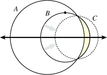
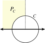
(a)	(b)	(c)

Figure 3: (a) The apex of each circle in the optimal cover lies outside the other circles. (b) The points $Y_{C}$ lie in the shaded region. (c) If $A$ and $C$ are adjacent circles in the optimal covering, the shaded region $B(A,C)$ is empty.

To compute the optimal cover of $Y$, it suffices to consider subproblems of the following form. For each pinned circle $C$, let $Y_{C}$ denote the set of clients outside $C$ and to the left of its center; see Figure 3(b). Then for each pinned circle $C$, we have $cost(Y_{C})=\min_{A}(f(radius(A))+cost(Y_{A}))$, where the minimum is taken over all pinned circles $A$ satisfying the following conditions: (1) The center of $A$ is left of the center of $C$; (2) the apex of $A$ is outside $C$; (3) the apex of $C$ is outside $A$; and (4) $A$ encloses every point in $Y_{C}\setminus Y_{A}$. The last condition is equivalent to there being no clients inside the region $B(A,C)$ bounded by the $x$-axis, the circles $A$ and $C$, and vertical lines through the apices of $A$ and $C$; see Figure 3(c).

Our dynamic programming algorithm (Figure 2 (right)) considers the pinned circles $C_{1},C_{2},\dots,C_{p}$ in left to right order by their centers; that is, the center of $C_{i}$ is left of the center of $C_{j}$ whenever $i<j$. To simplify notation, let $Y_{i}=Y_{C_{i}}$. For convenience, we add two circles $C_{0}$ and $C_{p+1}$ of radius zero, centered far to the left and right of $Y$, respectively, so that $Y_{0}=\varnothing$ and $Y_{p+1}=Y$.

Implementing everything using brute force, we obtain a running time of $O(n^{5})$. However, we can improve the running time to $O(n^{4}\log n)$ using the two-level data structure described in the previous section, together with a priority search tree. The region $B(C_{i},C_{j})$ can be partitioned into two or three three-sided regions, each bounded by two vertical lines and either a circular arc or the $x$-axis. We can test each three-sided region for emptiness in $O(\log n)$ time.

Theorem 3.0.

Let $f:{}_{+}\to\R$ be a fixed non-decreasing cost function. Given $n$ clients in the plane, we can compute in $O(n^{4}\log n)$ time a covering by circles (in any fixed $L_{p}$ metric) centered on the $x$-axis, such that the sum of the costs of the circles is minimized.

The algorithm is essentially unchanged in the $L_{\infty}$ metric, except now we define the apex of a square to be its upper right corner. It is easy to show that there is an optimal square cover in which no square contains the apex of any other square. Equivalently, we can assume without loss of generality that if two squares in the optimal cover overlap, the larger square is on the left. To compute the optimal cover, it suffices to consider subsets $Y_{C}$ of points either directly above or to the right of each pinned square $C$. For any two squares $A$ and $C$, the region $B(A,C)$ is now either a three-sided rectangle or the union of two three-sided rectangles, so we can use a simple priority search tree instead of our two-level data structure to test whether $B(A,C)$ is empty in $O(\log n)$ time.

However, one further observation does improve the running time by a linear factor: Without loss of generality, the rightmost box in the optimal cover of $Y_{C}$ has the rightmost point of $Y_{C}$ on its right edge. Thus, there are at most $n$ candidate boxes $C_{i}$ to test in the inner loop; we can easily enumerate these candidates in $O(n)$ time.

Theorem 3.0.

Let $f:{}_{+}\to\R$ be a fixed non-decreasing cost function. Given $n$ clients in the plane, we can compute in $O(n^{3}\log n)$ time a covering by axis-aligned squares centered on the $x$-axis, such that the sum of the costs of the squares is minimized.

3.1.2 Fast and simple solutions

In this section we describe simple and inexpensive algorithms that achieve constant factor approximations for finding a minimum-cost cover with disks centered along a fixed horizontal line $L$, using any $L_{p}$ metric. The main idea for the proofs of this section is to associate with a given disk $D$ in OPT, a set of disks in the approximate solution and argue that the set of associated disks cannot be more than a given constant factor cover of $D$, in terms of cumulative edge length, cumulative area, and so forth.

As in the previous section, the case of $L_{\infty}$ metric is the easiest to handle. By equivalence of all the $L_{p}$ metrics, constant-factor $c$-approximations for squares will extend to constant-factor $c^{\prime}$-approximations for $L_{p}$ disks.

Square Greedy Cover Algorithm (SG): Process the client points in order of decreasing distance from the line $L$. Find the farthest point $p_{1}$ from $L$; cover $p_{1}$ with a square $S_{1}$ exactly of the same height as $p_{1}$ centered at the projection of $p_{1}$ on $L$. Remove all points covered by $S_{1}$ from further consideration and recurse, finding the next farthest point from $L$ and so forth. In the case where two points are precisely the same distance from $L$, break ties arbitrarily.

Obviously, SG computes a valid covering of $Y$ by construction.We begin the analysis with a simple observation.

Lemma 3.1.

In the SG covering, any point in the plane (not necessarily a client) cannot be covered by more than two boxes.

Proof 3.2.

Suppose $S_{i}$ and $S_{j}$ are two squares placed during the running of SG and that $i<j$ so that $S_{i}$ was placed before $S_{j}$. Then $S_{i}$ cannot contain the center point of $S_{j}$ since then $S_{j}$ would not have had the opportunity to be placed, and similarly $S_{j}$ cannot contain the center point of $S_{i}$. Now consider a point $p\in S_{i}\cap S_{j}$. If $p$ were covered by a third square $S_{k}$ then either one of $\{S_{i},S_{j}\}$ would contain the center of $S_{k}$, or $S_{k}$ would contain the center of one of $\{S_{i},S_{j}\}$, neither of which is possible.

Theorem 3.2.

Given a set $Y$ of $n$ clients in the plane and any $\alpha\geqslant 1$, SG computes in time $O(n\log n)$ a covering of $Y$ by axis-aligned squares centered on the $x$-axis whose cost is at most three times the optimal.

Proof 3.3.

Let $Y=\{p_{1},\ldots,p_{n}\}$ and consider a square $S$ in OPT. We consider those squares $\{S_{i_{j}}\}$ selected by SG corresponding to points $\{p_{i_{j}}:p_{i_{j}}\in S\}$, see Figure 4,

Figure 4: Squares of the SG algorithm inside a square of the optimal solution.

and argue that these squares cannot have more than three times the total edge length of $S$. The same will then follow for all of SG and all of OPT. The argument, without modification, covers the case of cost measured in terms of the sum of edge length raised to an arbitrary positive exponent $\alpha\geq 1$.

Arguing as in Lemma 3.1 it is easy to see that at most two boxes $S_{i_{j}}$ associated with points $p_{i_{j}}\in S$ processed by SG actually protrude outside of $S$, one on the left and one on the right. Denote by $r$ the total horizontal length of these protruding parts of squares, then $r\leqslant s$, the side length of $S$, since the side length of each protruding square is at most $s$ and at most half of each square is protruding.

Because of Lemma 3.1 the total horizontal length of all nonprotruding parts of the squares $S_{i_{j}}$ is at most $2s$, consequently all points covered by $S$ in OPT are covered by a set of squares $S_{i_{j}}$ in SG whose total (horizontal) edge length $\sum_{j}s_{i_{j}}$ is at most $3s$.

For exponents $\alpha>1$ observe that $\sum_{j}s_{i_{j}}\leq 3s$ and $0\leq s_{i_{j}}\leq s$ for all $j$ implies that $\sum_{j}{s_{i_{j}}}^{\alpha}\leq 3s^{\alpha}$.

To analyze the running time of the algorithm we need some more details about the data structures used: Initially, sort the points by $x$-coordinate and separately by distance from the line $L$ in time $O(n\log{n})$ and process the points in order of decreasing distance from $L$. As the point $p_{i}$ at distance $d_{i}$ from $L$ is processed, we throw away points which are within horizontal distance $d_{i}$ from $p_{i}$. This takes time $O(\log{n}+k_{i})$ time where $k_{i}$ is the number of points within $d_{i}$ from $p_{i}$. Since we do this up to $n$ times with $k_{1}+\cdots+k_{l}=n$ the total running time is $O(n\log{n})$.

For the linear cost function, it is easy to modify the SG algorithm to get a $2$-approximation algorithm.

Square Greedy with Growth Algorithm (SGG): Process the points as in SG. However, if capturing a point $p_{i}$ by a square $S_{i}$ would result in an overlap with already existing square $S_{j}$ then, rather than placing $S_{i}$, grow $S_{j}$ just enough to capture $p_{i}$, keeping the vertical edge furthest from $p_{i}$ at the same point on $L$. If placing $S_{i}$ would overlap two squares, grow the one which requires the smallest edge extension. Break ties arbitrarily.

A proof somewhat similar to that of Lemma 2 shows that:

Theorem 3.3.

Given $n$ clients in the plane, SGG computes in time $O(n\log n)$ a covering by axis-aligned squares centered on the $x$-axis whose cumulative edge length is at most twice the optimal.

Proof 3.4.

As we process points $p_{i}$ using SGG, attribute to each point $p_{i}$ a line segment $s_{i}$ along $L$ as follows. If processing $p_{i}$ resulted in the placement of a square $S_{i}$ centered at the projection of $p_{i}$ in $L$ then attribute to $p_{i}$ the projection on $L$ of a horizontal edge of $S_{i}$ (Case 1). If, on the other hand, processing of $p_{i}$ resulted in the growing of a prior square $S_{j}$ to just capture $p_{i}$, attribute to $p_{i}$ the projection on $L$ of the portion of the horizontal edge of the expanded $S_{j}$ needed to capture $p_{i}$ (Case 2). (This amount is at most the distance of $p_{i}$ to $L$ since otherwise $p_{i}$ would have been fallen into case 1.) We must show that the lengths of the segments is no more than twice the edge lengths of squares in OPT.

It suffices to show that for any square $S$ in OPT, the segments $s_{i}$ associated with points $p_{i}\in S$ processed by SGG cannot have total edge length which exceeds twice the edge length $s$ of $S$.

To see this observe that the sum of the lengths of those $s_{i}$ lying completely inside $S$ does not exceed $s$ since they are nonoverlapping. In addition, each of the parts of the at most two segments protruding from $S$ can have length at most $s/2$, in case 1 for the same reason as in the SG algorithm, in case 2 since the total length of the segment is at most $s/2$.

In order to make SGG efficient, we proceed as in SG. In addition, we maintain a balanced binary search tree containing the $x$-coordinates of the vertical sides of the squares already constructed. For each new point $p_{i}$ to be processed we locate its $x$-coordinate within this structure to obtain its neighboring squares and to decide whether case 1 or case 2 applies. This can be done in time $O(\log n)$ just as adding a new square in case 1 or updating an existing square in case 2. Removing points covered by the new or updated square is done as in SG, so that the total runtime remains $O(n\log n)$.

Unlike SG, SGG is not a constant factor approximation for area. Consider $n$ consecutive points at height $1$ separated one from the next by distance of $1+\epsilon$. Processing the points left to right using SGG covers all points with one square of edge length $n+(n-1)\epsilon$, and so area $O(n^{2})$, while covering all points with $n$ overlapping squares each of edge length $2$, uses total area $4n$.

Finally, extending these results from squares to disks in any $L_{p}$ metric is not difficult. Enclosing each square in the algorithm by an $L_{p}$ disk leads to an approximation factor $3c^{2}$ for GG and $2c^{2}$ for SGG, where $c=p^{\alpha/p}$. In particular, for $L_{2}$ disks, this yields a $2\sqrt{2}$-approximation for $\alpha=1$ and a $4$-approximation for $\alpha=2$.

3.2 Finding the best axis-parallel line

When the horizontal line $\ell$ is not given but its orientation is fixed, we first prove that finding the best line, even for $\alpha=1$, is uncomputable, then in this linear case give a simple approximation, and finally a PTAS.

3.2.1 A hardness result – uncomputability by radicals

Our approach is similar to the approach used by Bajaj on the unsolvability of the Fermat-Weber problem and other geometric optimization problems[5, 6].

Theorem 3.4.

Let $c(t)=\sum_{i}{r_{i}}$ denote the minimum cost of a cover whose centers lie on the line of equation $y=t$. There exists a set $Y$ of clients such that, if $t_{0}$ is the value that minimizes $c(t)$, then $t_{0}$ is uncomputable by radicals.

The proof proceeds by exhibiting such a point set and showing by differentiating $c(t)$ that $t_{0}$ is the root of a polynomial which is proven not to be solvable by radicals.

The following definitions and facts can be found in a standard abstract algebra reference; see, for example, Rotman[22]. A polynomial with rational coefficients is solvable by radicals if its roots can be expressed using rational numbers, the field operations, and taking $k$th roots. The splitting field of a polynomial $f(x)$ over the field of rationals is the smallest subfield of the complex numbers containing all of the roots of $f(x)$. The Galois group of a polynomial $f(x)$ with respect to the coefficient field is the group of automorphisms of the splitting field that leave fixed. If the Galois group of $f(x)$ over is a symmetric group on five or more elements, then $f(x)$ is not solvable by radicals over .

Consider the following set of points:$\{(3,4),(-3,-2),(102,2),$ $(98,-2),(200,-2)\}$. By exhaustive case analysis, we can show that the optimal solution must consist of one circle through the first two points, a second circle through the next two points, and a third circle touching the last point, and the optimal horizontal line must lie in the range $-2\leq y\leq 2$. For a given value of $y$ in this range, the cost of the best cover is

$$c(y)=\sqrt{2(y-1)^{2}+18}+\sqrt{2y^{2}+8}+(2-y).$$

Therefore, in order to find the best horizontal line, we must minimize $c(y)$. Setting the derivative to zero, we obtain the equation

$$c^{\prime}(y)=\frac{2(y-1)}{\sqrt{2(y-1)^{2}+18}}+\frac{2y}{\sqrt{2y^{2}+8}}-1=0.$$

We easily verify that $c^{\prime\prime}(y)$ is always positive. The minimum value $c(y)\approx 8.3327196$ is attained at $y\approx 1.4024709$, which is a root of the following polynomial:

$$f(y) = 1024+512y-1600y^{2}+1536y^{3}-960y^{4}$$

$$+368y^{5}-172y^{6}+28y^{7}-7y^{8}.$$

Using the computational system GAP[15], we compute that the Galois group of $f(y)$ is the symmetric group $S_{8}$, so the polynomial is not solvable by radicals.

3.2.2 Fast and simple constant-factor approximations

The simple constant factor approximations for a fixed line can be extended to the case of approximations to the optimal solution on an arbitrary axis-parallel line with the same constant factors, though with a multiplicative factor of $O(n^{2})$ increase in running time.

3.2.3 An FPTAS for finding the best horizontal line

We begin with the case $\alpha=1$. Let $d$ denote the distance between the highest and lowest point. Clearly, $d/2\leqslant$ OPT $\leqslant nd/2$. Partition the horizontal strip of height $d$ that covers the points into $2n/\epsilon$ horizontal strips, each of height $\delta=d\epsilon/2n$, using $2n/\epsilon-1$ regularly-spaced horizontal lines, $\ell_{i}$. For each line $\ell_{i}$, we run the exact dynamic programming algorithm, and keep the best among these solutions. Consider the line, $\ell^{*}$, that contains OPT. We can shift line $\ell^{*}$ to the nearest $\ell_{i}$, while increasing the radius of each disk of OPT by at most $\delta$, to obtain a covering of the points by disks centered on some $\ell_{i}$; the total increase in cost is at most $\delta n=d\epsilon/2\leqslant\epsilon$ OPT. Thus, our algorithm computes a $(1+\epsilon)$-approximation in time $O((n^{3}/\epsilon)\log{n})$.

In order to generalize this result to the case $\alpha>1$, let us write PSEUDO-OPT for the lowest cost of a solution on any of the horizontal lines $\ell_{i}$, SHIFT for the result of shifting OPT to the closest of these lines, and $r_{1},...,r_{m}$ for the radii of the optimal set of disks. For an arbitrary power $\alpha\geq 1$, we have

PSEUDO-OPT $$\leq \mbox{SHIFT}\leq\sum_{i=1}^{m}(r_{i}+\delta)^{\alpha}$$

$$\leq \sum_{i=1}^{m}r_{i}^{\alpha}+\delta\alpha\sum_{i=1}^{m}(r_{i}+\delta)^{\alpha-1}$$

$$\leq \mbox{OPT}(1+\delta\alpha 2^{2\alpha-1}n/d).$$

The last line uses $\delta\leq d,r_{i}\leq d$ and $\mbox{OPT}\geq(d/2)^{\alpha}$. Choosing $\delta=\varepsilon d/(\alpha 2^{2\alpha-1}n)$ gives the desired $(1+\varepsilon)$-approximation.

Together with the results from previous sections we have:

Theorem 3.4.

Given $n$ clients in the plane and a fixed $\alpha\geqslant 1$, there exists an FPTAS for finding an optimally positioned horizontal line and a minimum-cost covering by disks centered on that line. It runs in time $O((n^{3}/\epsilon)\log n)$ for the linear cost case ($\alpha=1$) and $O((n^{5}/\epsilon)\log n)$ for $\alpha>1$.

3.3 Approximating the best line –
any orientation

Finally, we sketch approximation results for selecting the best line whose orientation is not given. We give both a constant factor approximation and a PTAS for the linear cost case ($\alpha=1$).

3.3.1 Fast and simple constant-factor approximations

Given a line $\ell$, we say that a set $\mathcal{D}$ of disks $D_{1}$,…,$D_{k}$ is $\ell$-centered if the centers of every disk $C_{j}$ in $\mathcal{D}$ belongs to $\ell$. Recall that the cost of $\mathcal{D}$ is the sum of all its radii.

Lemma 3.5.

Given $k\geqslant 1$, a line $\ell$, an $\ell$-centered set $\mathcal{D}$ of $k$ disks that cover $Y$, and any point $p_{0}$ on $\ell$, there exist $p^{\prime}\in Y$ and an $\ell^{\prime}$-centered set $\mathcal{D}^{\prime}$ of $k$ disks that cover $Y$, where $\ell^{\prime}$ is the line that joins $p_{0}$ and $p^{\prime}$, such that the cost of $\mathcal{D}^{\prime}$ is at most $2^{\alpha}$ times the cost of $\mathcal{D}$.

Proof 3.6.

We will assume without loss of generality that $\ell$ is the $x$-axis, $p_{0}$ is the origin and that no other point in $Y$ lies on the $y$-axis. The latter restriction can easily be enforced by a small perturbation. Let the coordinates of $p_{i}$ be $x_{i}$ and $y_{i}$, and let $m_{i}$ denote the slope $y_{i}/x_{i}$ of the line $\ell_{i}$ for $1\leqslant i\leqslant n$. First, we reorder $Y$ so that $|m_{1}|\leqslant\dots\leqslant|m_{n}|$. In what follows we assume that $x_{1}>0$ and $y_{1}\geqslant 0$. The other cases can be treated analogously.

For each disk $D_{j}=D(t_{j},r_{j})$ in $\mathcal{D}$, we construct a disk $D^{\prime}_{j}$ whose radius is $r^{\prime}_{j}=2r_{j}$ and center $t^{\prime}_{j}$ is obtained from $t_{j}$ by rotating it around the origin counterclockwise by an angle $\tan^{-1}(m_{1})$. The set $\mathcal{D}^{\prime}$ of $k$ disks thus defined is $\ell^{\prime}$-centered, where $\ell^{\prime}=\{(x,y)\in{}^{2}\mid y=m_{1}x\}$ and $p_{1}\in\ell^{\prime}$. To see that $\mathcal{D}^{\prime}$ covers $Y$, simply observe that $d(t_{j},t^{\prime}_{j})\leqslant r_{j}$ for all $1\leqslant j\leqslant k$ and apply the triangle inequality: any point in $D_{j}$ must be at distance at most $2r_{j}$ of $t^{\prime}_{j}$. The cost of this new solution is clearly at most $2^{\alpha}$ times that of $\mathcal{D}$ in the linear cost case.

By a double appplication of this lemma, first about an arbitrary $p_{0}$ yielding a point $p^{\prime}=p_{i}$, then about $p_{i}$ yielding another $p^{\prime}=p_{j}$, it is immediate that any $\ell$-centered cover of $Y$ can be transformed into an $\ell_{i,j}$-centered cover whose cost is increased at most four-fold, where $\ell_{i,i}$ is the line joining $p_{i}$ and $p_{j}$. By computing (exactly or approximately) the optimal set of disks for all $O(n^{2})$ lines defined by two different points of $Y$, we conclude:

Theorem 3.6.

Given $n$ clients in the plane and a fixed $\alpha\geqslant 1$, in $O(n^{4}\log n)$ time, we can find a collinear set of disks that cover $P$ at cost at most $4^{\alpha}OPT$, and for $\alpha=1$, in $O(n^{3}\log n)$ time, we can find a collinear set of disks that cover $P$ at cost at most $8\sqrt{2}OPT$.

3.3.2 A PTAS for finding the best line with
unconstrained orientation

We now prove that finding the best line with unconstrained orientation and a minimum-cost covering with disks whose centers are on that line admits a PTAS.

Theorem 3.6.

Let $Y$ be a set of $n$ clients in the plane that can be covered by an optimal collinear set of disks at linear cost $OPT$ (i.e., $\alpha=1$), and $\epsilon>0$. In $O((n^{4}/\epsilon^{2})\log n)$ time, we can find a collinear set of disks that cover $Y$ at cost at most $(1+\epsilon)OPT$.

Proof 3.7.

Let $H$ be a strip of minimal width $h$ that contains $Y$. Using a rotating calipers approach, $H$ can be computed in $O(n\log n)$ time. If $h=0$, we can conclude that $OPT=0$ and we are done.

Otherwise, we can assume wlog that $H$ is horizontal and that its center line is the $x$-axis. Let $R$ denote the smallest enclosing axis-parallel rectangle $R$ of $Y$, $w$ its width, and $h$ its height, Then $h\leq w$ and, moreover, $h/2\leqslant OPT$. Let $\ell^{*}$ be the optimal line.

We now distinguish two cases:

Case 1. $w\geqslant 2h$: Observe that both vertical sides $v_{1},v_{2}$ of $R$ contain a point of $Y$. Therefore, $\ell^{*}$ must have distance at most $OPT$ to $v_{1}$ and $v_{2}$. A straightforward calculation shows that then $\ell^{*}$ must intersect the lines $\ell_{1}$ and $\ell_{2}$ extending $v_{1}$ and $v_{2}$ at a distance of at most $4OPT$ from the $x$-axis.

The idea is now to put points on those parts of $\ell_{1}$ and $\ell_{2}$ which are equally spaced at distance $\delta=\varepsilon OPT/n$. Then we consider all lines passing through one of these points on $\ell_{1}$ and one on $\ell_{2}$. For each such line we find the optimal covering of $P$ by circles centered on it using the algorithm of Theorem 3.0, and give out the best one as an approximation for the optimum.

Observe, that there is one of the lines checked, $\hat{\ell}$, whose intersection points with $\ell_{1}$ and $\ell_{2}$ are at distance at most $\delta/2$ from the ones of $\ell^{*}$. Elementary geometric considerations show that to any point $p$ in $\ell^{*}$ closest to some point of $P$ there is a point in $\hat{\ell}$ within distance at most $\delta$. Consequently, to any circle of radius $r$ of the optimal covering centered on $\ell^{*}$, there is a circle on $\hat{l}$ of radius $r+\delta$ covering the same set of points (or more). Thus, $\hat{l}$ has a covering that differs by at most $n\delta$ from the optimal one. By the choice of $\delta$ we have a $1+\varepsilon$-approximation to the optimum.

Observe, that we chose $O(OPT/\delta)=O(n/\varepsilon)$ points on $\ell_{1}$ and $\ell_{2}$, so we are checking $O((n/\varepsilon)^{2})$ lines. For each of them, we apply the algorithm of Theorem 3.0 which has runtime $O(n^{2}\log n)$ yielding a total runtime of $O(n^{4}/{\varepsilon^{2}}\log n)$.

Case 2. $w<2h$: In this case the optimal line $\ell^{*}$ can have a steeper slope and even be vertical. Of course, it must intersect $R$ and we expand $R$ to a cocentric rectangle $R^{\prime}$ such that the footpoint of any point in $Y$ on $\ell^{*}$ must lie inside $R^{\prime}$. An easy geometric consideration shows that extending the width of $R$ by $h$ and its height by $w$ will suffice, so $R^{\prime}$ is a square of side length $w+h$. Then we put equally spaced points of distance $\delta=\varepsilon OPT/n$ on the whole boundary of $R^{\prime}$, apply the algorithm of Theorem 3.0 to all lines passing through any two of these points, and return the one giving the smallest covering as an approximation to the optimum. The same consideration as in the first case shows that this is indeed a $(1+\varepsilon)$-approximation. Since the length of the boundary of $R^{\prime}$ is $4(w+h)\leqslant 12h\leqslant 24OPT$, we obtain the desired runtime in this case, as well.

For both cases it remains to show how to obtain a suitable value of $\delta$, since we do not know the value of $OPT$. Since any value below $OPT$ suffices, we simply run a constant factor $c$ approximation algorithm of Theorem 3.0 and take $1/c$ times the value it returns instead of $OPT$ in the definition of $\delta$.

4 Minimum-Cost Covering Tours

We now consider the minimum cost covering tour (MCCT) problem: Given $k\geqslant 1$ and a set $Y=\{p_{1},\ldots,p_{n}\}$ of $n$ clients, determine a cover of $Y$ by (at most) $k$ disks centered at $X=\{t_{1},\ldots,t_{k}\}$ with radii $r_{j}$ and a tour $T$ visiting $X$, such that the cost $\mathrm{length}(T)+C\sum r_{i}^{\alpha}$ is minimized. We refer to the tour $T$, together with the disks centered on $X$, as a covering tour of $Y$. Our results are for the case of linear transmission costs ($\alpha=1$). We first show a weak hardness result, then characterize the solution for $C\leqslant 4$, and finally give a PTAS for a fixed $C>4$.

4.1 A hardness result

We prove the NP-hardness of MCCT where $C$ is also part of the input. Note that this does not prove the NP-hardness of MCCT where $C$ is a fixed constant, which is the problem for which we give a PTAS below. Note also that $C$ appears in the run time exponent of that PTAS, and so the PTAS no longer runs in polynomial time if $C$ is not a fixed constant.

Theorem 4.0.

MCCT with linear cost is NP-hard if the ratio $C$ is part of the input.

Proof (sketch).  We show a reduction from Hamilton cycle in grid graphs. Given a set of $n$ points on a grid, we construct an instance of MCCT in which each of the given points is a client. We set $C$ to be larger than $2n$. We claim that the grid graph has a Hamilton cycle if and only if there is a tour $T$ visiting a set of disk centers with radii $r_{i}$ whose cost is at most $n$.

Clearly a Hamilton cycle in the grid graph yields a tour of cost $n$ with each client contained in a disk of radius 0 centered at that point.

Conversely, suppose we have a tour whose cost (length plus sum of radii) is at most $n$. Note that no two clients can be contained in a single disk, as such a disk must have radius at least 0.5, and thus its contribution to the cost $C\cdot r_{i}>2n\cdot 0.5=n$ contrary to our assumption. Next we want to show that each disk in an optimal solution is centered at the client it covers. Suppose this is not the case, there is some client $j$ which is covered by a disk centered at $c_{j}\not=j$. Let the distance between client $j$ and the center of the disk covering it be $d$. Now consider an alternate feasible solution in which the tour visits $c_{j}$ then $j$ then back to $c_{j}$, covering $j$ with a disk of radius 0. No other client is affected by this change, as the disk only covers point $j$. The cost of the new solution is the cost of the original (optimal) solution $+2d-Cd$ as we add $2d$ to the length of the tour, but decrease $C\sum r_{i}$ by $Cd$. Since $C>2$ the new solution is better than the original optimal solution, a contradition.∎

4.2 The case $C\leqslant 4$: The exact solution is
a single circle

Theorem 4.0.

In the plane, with a cost function of $\mathrm{length}(T)+C\sum r_{i}$ and $C\leqslant 4$, the minimum-cost solution is to broadcast to all clients from the circumcenter of the client locations and no tour cost.

The proof rests on the following elementary geometry lemma (whose proof is omitted here).

Lemma 4.1.

For three points $p$, $q$ and $r$ in the plane, such that the triangle $pqr$ contains its own circumcenter, the length of a trip from $p$ to $q$ to $r$ and back to $p$ is at least $4r$ where $r$ is the circumradius of the points.

Proof of Theorem 4.0.  Let $r(X)$ and $r(Y)$ denote the minimum radius of a circle enclosing $X$ or $Y$, respectively. Let $T$ be a covering tour of $Y$, $X\subseteq T$ be the set of disk centers and $r_{j}$ their radii. Finally, let $r_{\mathrm{max}}=\max_{j}r_{j}$.

By the triangle inequality, Lemma 4.1 implies that the $\mathrm{length}(T)\geqslant 4r(X)$. Since the tour visits all the centers in $X$ and the disks centered at $X$ cover $Y$, we have $r(Y)\leqslant r(X)+r_{\mathrm{max}}$. By definition, the cost of $T$ is $\mathrm{length}(T)+C\sum_{j}{r_{j}}$, which by the observation above is at least $4r(X)+C\sum_{j}{r_{j}}\geqslant 4r(X)+Cr_{\mathrm{max}}$. The assumption $C\leqslant 4$ then implies that it be at least $C(r(X)+r_{\mathrm{max}})\geqslant Cr(Y)$, which is the cost of covering by a single disk with a zero-length tour. ∎

4.3 The case $C>4$: A PTAS

We distinguish between two cases for the choice of transmission points: they may either be arbitrary points in the plane (selected by the algorithm) or they may be constrained to lie within a discrete set ${\cal T}$ of candidate locations.

The constant $C$ specifies the relative weight associated with the two parts of the cost function – the length of the tour, and the sum of the disk radii. If $C$ is very small ($C\leqslant 4$), then the solution is to cover the set $Y$ using a single disk (the minimum enclosing disk), and a corresponding tour of length 0 (the singleton point that is the center of the disk). If $C$ is very large, then the priority is to minimize the sum of the radii of the $k$ disks. Thus, the solution is to compute a covering of $Y$ by $k$ disks that minimizes the sum of radii (as in[19]), and then link the resulting disk centers with a traveling salesman tour (TSP). (In the case that $k\geqslant n$, the disks in the covering will be of radius 0, and the problem becomes that of computing a TSP tour on $Y$.) Note that our algorithm gives an alternative to the Lev-Tov and Peleg PTAS[19] for coverage alone.

Our algorithm is based on applying the $m$-guillotine method[20], appropriately adapted to take into account the cost function and coverage constraint. We need several definitions; we largely follow the notation of [20]. Let $G=(V,E)$ be an embedding of a connected planar graph, of total Euclidean edge-length $L$. Let ${\cal D}$ be a set of disks centered at each vertex $v$ of $G$ of radius $r_{v}$. We refer to the pair $(G,{\cal D})$ as a covering network if the union $\cup_{v\in V}D_{v}$ of the disks covers the clients $Y$. We can assume without loss of generality that $G$ is restricted to the unit square $B$, i.e., $\cup_{e\in E}e\subset int(B)$.

Our algorithm relies on there being a polynomial-size set of candidate locations for the transmission points that will serve as the vertices of the covering tour we compute. In the case that a set ${\cal T}$ of candidate points is given, this is no issue; however, in the case that the transmission points are arbitrary, we appeal to the following grid-rounding lemma (proved in the full paper).

Lemma 4.2.

One can perturb any covering network $(G,{\cal D})$ to have its vertices all at grid points on a regular grid of spacing $\delta=O(\epsilon\cdot diam(S)/n)$, while increasing the total cost by at most a factor of $(1+\epsilon)$.

An axis-aligned rectangle, $W\subseteq B$, is called a window; rectangle $W$ will correspond to a subproblem in a dynamic programming algorithm. An axis-parallel line $\ell$ that intersects $W$ is called a cut.

For a covering network with edge set $E$ and a set of disks ${\cal D}$, we say that $(E,{\cal D})$ satisfies the $m$-guillotine property with respect to window $W$ if either (1) all clients $Y\subset W$ lie within disks of ${\cal D}$ that intersect the boundary of $W$; or (2) there exists a cut $\ell$ with certain properties (an $m$-good cut with respect to $W$) that splits $W$ into $W_{1}$ and $W_{2}$, and $(E,{\cal D})$ recursively satisfies the $m$-guillotine property with respect to both $W_{1}$ and $W_{2}$. Due to the lack of space, we cannot give the full definition of an $m$-good cut (see the full paper).

The crux of the method is a structural theorem, which shows how to convert any covering network $(G,{\cal D})$ into another covering network $(G^{\prime},{\cal D}^{\prime})$, such that the new graph $G^{\prime}$ satisfies the $m$-guillotine property, and that the total cost of the new instance $(G^{\prime},{\cal D}^{\prime})$ is at most $O((L+CR)/m)$ times greater than the original instance $(G,{\cal D})$, where $L$ is the total edge length of $G$ and $R$ the sum of the radii of ${\cal D}$. The construction is recursive: at each stage, we show that there exists a cut with respect to the current window $W$ (which initially is the unit square $B$), such that we can “afford” (by means of a charging scheme) to add short horizontal/vertical edges in order to satisfy the $m$-guillotine property, without increasing the total edge length too much.

We then apply a dynamic programming algorithm, running in $O(n^{O(m)})$ time, to compute a minimum-cost covering network having a prescribed set of properties: (1) it satisfies the $m$-guillotine property (with respect to $B$), which is necessary for the dynamic program to have the claimed efficiency; (2) its disks cover the clients $Y$; and (3) its edge set contains an Eulerian subgraph. This third condition allows us to extract a tour in the end. In the proof of the following theorem (see the full paper), we give the details of the dynamic programming algorithm that yields:

Theorem 4.2.

The min-cost covering tour problem has a PTAS that runs in time $O(n^{O(1/\epsilon)})$.

References

- [1] P. K. Agarwal and M. Sharir. Efficient algorithms for geometric optimization. ACM Computing Surveys, 30(4):412–458, 1998.
- [2] E. M. Arkin, S. P. Fekete, and J. S. B. Mitchell. Approximation algorithms for lawn mowing and milling. Comput. Geom.: Theory Appl., 17(1–2):25–50, 2000.
- [3] E. M. Arkin and R. Hassin. Approximation algorithms for the geometric covering salesman problem. Discrete Applied Math., 55(3):197–218, 1994.
- [4] S. Arora, P. Raghavan, and S. Rao. Approximation schemes for Euclidean -medians and related problems. In Proc. 30th Annu. ACM Symp. Theory Computing, pages 106–113, 1998.
- [5] C. Bajaj. Proving geometric algorithm non-solvability: An application of factoring polynomials. J. Symbol. Comput., 2(1):99–102, 1986.
- [6] C. Bajaj. The algebraic degree of geometric optimization problems. Discrete & Comput. Geom., 3:177–191, 1988.
- [7] V. Bilò, I. Caragiannis, C. Kaklamanis, and P. Kanellopoulos. Geometric clustering to minimize the sum of cluster sizes. In Proc. 13th European Symp. Algorithms, Vol 3669 of LNCS, pages 460–471, 2005.
- [8] H. Brönnimann and M. T. Goodrich. Almost optimal set covers in finite VC-dimension. Discrete & Comput. Geom., 14(4):463–479, 1995.
- [9] M. Charikar and R. Panigrahy. Clustering to minimize the sum of cluster diameters. J. Computer Systems Sci., 68(2):417–441, 2004.
- [10] A. E. F. Clementi, P. Penna, and R. Silvestri. On the power assignment problem in radio networks. Technical Report TR00-054, Electronic Colloquium on Computational Complexity, 2000.
- [11] A. Dumitrescu and J. S. B. Mitchell. Approximation algorithms for TSP with neighborhoods in the plane. J. Algorithms, 48(1):135–159, 2003.
- [12] T. Erlebach, K. Jansen, and E. Seidel. Polynomial-time approximation scheme for geometric graphs. SIAM J. Computing, 34(6):1302–1323, 2005.
- [13] S. P. Fekete, R. Klein, and A. Nüchter. Searching with an autonomous robot. In Proc. 20th ACM Annu. Symp. Comput. Geom., pages 449–450, 2004. Video available at http://compgeom.poly.edu/acmvideos/socg04video/.
- [14] S. P. Fekete, R. Klein, and A. Nüchter. Online searching with an autonomous robot. In Algorithmic Foundations of Robotics VI, Vol 17 of Tracts in Advanced Robotics, pages 139–154. Springer, Berlin, 2005.
- [15] The GAP Group. GAP – Groups, Algorithms, and Programming, Version 4.4, 2005. http://www.gap-system.org.
- [16] T. F. Gonzalez. Covering a set of points in multidimensional space. Inf. Proc. Letters, 40(4):181–188, 1991.
- [17] J. Hershberger. Minimizing the sum of diameters efficiently. Comput. Geom.: Theory Appl., 2(2):111–118, 1992.
- [18] D. S. Hochbaum and W. Maass. Approximation schemes for covering and packing problems in image processing and VLSI. J. ACM, 32(1):130–136, 1985.
- [19] N. Lev-Tov and D. Peleg. Polynomial time approximation schemes for base station coverage with minimum total radii. Computer Networks, 47(4):489–501, 2005.
- [20] J. S. B. Mitchell. Guillotine subdivisions approximate polygonal subdivisions: A simple polynomial-time approximation scheme for geometric TSP, -MST, and related problems. SIAM J. Computing, 28(4):1298–1309, 1999.
- [21] K. Pahlavan and A. H. Levesque. Wireless information networks, Vol 001. Wiley, New York, NY, 2nd ed., 2005.
- [22] J. J. Rotman. Advanced Modern Algebra. Prentice Hall, 2002.