A Feedback Reduction Technique for
MIMO Broadcast Channels

Abstract

A multiple antenna broadcast channel with perfect channel state information at the receivers is considered. If each receiver quantizes its channel knowledge to a finite number of bits which are fed back to the transmitter, the large capacity benefits of the downlink channel can be realized. However, the required number of feedback bits per mobile must be scaled with both the number of transmit antennas and the system SNR, and thus can be quite large in even moderately sized systems. It is shown that a small number of antennas can be used at each receiver to improve the quality of the channel estimate provided to the transmitter. As a result, the required feedback rate per mobile can be significantly decreased.

I Introduction

In multiple antenna broadcast (downlink) channels, capacity can be tremendously increased by adding antennas at only the access point (transmitter) [1][2]. However, the transmitter must have accurate channel state information (CSI) in order to realize these multiplexing gains. In frequency-division duplexed systems, training can be used to obtain channel knowledge at each of the mobile devices (receivers), but obtaining CSI at the access point generally requires feedback from each mobile.

In the practically motivated finite rate feedback model, each mobile feeds back a finite number of bits regarding its channel instantiation at the beginning of each block or frame. The feedback bits are determined by quantizing the channel vector to one of $2^{B}$ quantization vectors. A downlink channel with such a feedback mechanism was analyzed in [3][4]. While only a few feedback bits suffice to obtain near-perfect CSIT performance in point-to-point MISO (multiple-input, single-output) channels [5][6], considerably more feedback is required in downlink channels. In fact, the feedback load per mobile must be scaled with the number of transmit antennas as well as the system SNR in downlink channels in order to achieve rates close to those achievable with perfect CSIT. In [3], it is shown that the following scaling of feedback bits per mobile

$$B=\frac{M-1}{3}P_{dB}$$ (1)

suffices to maintain a maximum gap of 3 dB between perfect CSIT and limited feedback performance. This feedback load, however, can be prohibitively large for even reasonable size systems. In a 10 antenna system operating at 10 dB, for example, this equates to 30 feedback bits per mobile.

In this paper, we propose a method that significantly reduces the required feedback load by utilizing a small number of receive antennas (denoted by $N$) at each mobile. The multiple receive antennas are not used to increase the number of data streams received at each mobile, as they are in point-to-point MIMO systems, but instead are used to improve the quality of the channel estimate provided to the transmitter. Each mobile linearly combines the received signals on its $N$ antennas to produce a scalar output, thereby creating an effective single antenna channel at each mobile. Transmission is then performed as in a multiple transmit antenna, single receive antenna downlink channel. However, the coefficients of the linear combiner at each mobile are not arbitrary, but instead are chosen to produce the effective single antenna channel that can be quantized with minimal error, thereby decreasing the quantization error for each mobile. Increasing the number of receive antennas $N$ clearly increases the space of possible effective channels, and thus leads to reduced quantization error. In a 10 antenna system operating at 10 dB, for example, this method reduces the feedback from 30 bits per mobile in the $N=1$ scenario to 25 bits and 21 bits, for $N=2$ and $N=3$, respectively.

Notation: We use lower-case boldface to denote vectors, upper-case boldface for matrices, and the symbol $(\cdot)^{H}$ for the conjugate transpose. The norm of vector ${\mathbf{x}}$ is denoted $||{\mathbf{x}}||$.

II System Model

We consider a $K$ receiver multiple antenna broadcast channel in which the transmitter (access point) has $M$ antennas, and each of the receivers has $N$ antennas. The received signal at the $i$-th antenna is described as:

$$y_{i}={\mathbf{h}}_{i}^{H}{\mathbf{x}}+n_{i},~{}~{}~{}i=1,\ldots,NK$$ (2)

where ${\bf h}_{1},{\bf h}_{2},\ldots,{\bf h}_{KN}$ are the channel vectors (with ${\bf h}_{i}\in{\mathbb{C}}^{M\times 1}$) describing the $KN$ receive antennas, the vector ${\bf x}\in{\mathbb{C}}^{M\times 1}$ is the transmitted signal, and ${\bf n}_{1},\ldots,{\mathbf{n}}_{NK}$ are independent complex Gaussian noise terms with unit variance. Note that receiver 1 has access to signals $y_{1},\ldots,y_{N}$, receiver 2 has access to $y_{N+1},\ldots,y_{2N}$, and the $i$-th receiver has access to $y_{(i-1)N+1},\ldots,y_{Ni}$. There is a transmit power constraint of $P$, i.e. we must satisfy $E[||{\mathbf{x}}||^{2}]\leq P$. We use ${\bf H}_{i}$ to denote the concatenation of the $i$-th receiver’s channels, i.e. ${\bf H}_{i}=[{\bf h}_{(i-1)N+1}\cdots{\bf h}_{Ni}]$. For simplicity of exposition we assume that the number of mobiles is equal to the number of transmit antennas, i.e., $K=M$. The results can easily be extended to the case where $K<M$, and the proposed technique can be combined with user selection when $K>M$. Furthermore, the number of receive antennas is assumed to be no larger than the number of transmit antennas.

We consider a block fading channel, with independent Rayleigh fading from block to block. Each of the receivers is assumed to have perfect and instantaneous knowledge of its own channel ${\bf H}_{i}$. Notice it is not required for mobiles to know the channel of other mobiles. In this work we study only the ergodic capacity, or the average rates achieved over an infinite number of blocks (or channel realizations).

II-A Finite Rate Feedback Model

Here we briefly describe the feedback model for a single receive antenna ($N=1$). At the beginning of each block, each receiver quantizes its channel (with ${\bf h}_{i}$ assumed to be known perfectly at the $i$-th receiver) to $B$ bits and feeds back the bits perfectly and instantaneously to the access point. Vector quantization is performed using a codebook ${\mathcal{C}}$ that consists of $2^{B}$ $M$-dimensional unit norm vectors ${\mathcal{C}}\triangleq\{\mathbf{w}_{1},\ldots,\mathbf{w}_{2^{B}}\}$, where $B$ is the number of feedback bits. Each receiver quantizes its channel vector to the beamforming vector that forms the minimum angle to it, or equivalently that maximizes the inner product [7] [8]. Thus, user $i$ quantizes its channel to $\hat{{\bf h}}_{i}$, chosen according to:

$$\hat{{\bf h}}_{i} = \textrm{arg}\max_{{\bf w}={\bf w}_{1},\ldots,{\bf w}_{2^{B}}}|{\mathbf{h}}_{i}^{H}{\bf w}|$$ (3)

$$= \textrm{arg}\min_{{\bf w}={\bf w}_{1},\ldots,{\bf w}_{2^{B}}}\sin^{2}\left(\angle({\bf h}_{i},{\bf w})\right).$$ (4)

and feeds the index of the quantization back to the transmitter. It is important to notice that only the direction of the channel vector is quantized, and no magnitude information is conveyed to the transmitter. The quantization error can be thought of as either the angle between the channel and its quantization $\angle({\bf h}_{i},\hat{{\bf h}}_{i})$ or the quantity $\sin^{2}(\angle({\bf h}_{i},\hat{{\bf h}}_{i}))$.

In this work we use random vector quantization (RVQ), in which each of the $2^{B}$ quantization vectors is independently chosen from the isotropic distribution on the $M$-dimensional unit sphere [5]. To simplify analysis, each receiver is assumed to use a different and independently generated codebook. We analyze performance averaged over all such choices of random codebooks. Random codebooks are used because the optimal vector quantizer for this problem is not known in general and known bounds are rather loose, whereas RVQ is amenable to analysis and also provides performance that is measurably close to the optimal [5].

II-B Zero-Forcing Beamforming

After receiving the quantization indices from each of the mobiles, the AP can use zero-forcing beamforming (ZFBF) to transmit data to the $M$ users. Let us again consider the $N=1$ scenario, where the channels are the vectors ${\bf h}_{1},\ldots,{\bf h}_{M}$. Since the transmitter does not have perfect CSI, ZFBF must be performed based on the quantizations instead of the actual channels. When ZFBF is used, the transmitted signal is defined as ${\bf x}=\sum_{i=1}^{M}x_{i}{\bf v}_{i}$, where each $x_{i}$ is a scalar (chosen complex Gaussian with power $P/M$) intended for the $i$-th receiver, and ${\bf v}_{i}\in{\mathcal{C}}^{M}$ is the beamforming vector for the $i$-th receiver. The beamforming vectors ${\bf v}_{1},\ldots,{\bf v}_{M}$ are chosen as the normalized rows of the matrix $[\hat{{\bf h}}_{i}\cdots\hat{{\bf h}}_{M}]^{-1}$, i.e., they satisfy $||{\bf v}_{i}||=1$ for all $i$ and $\hat{{\bf h}}_{i}^{H}{\bf v}_{j}=0$ for all $j\neq i$. If all multi-user interference is treated as additional noise, the resulting SINR at the $i$-th receiver is given by:

$$SINR_{i}=\frac{\frac{P}{M}|{\bf h}_{i}^{H}{\bf v}_{i}|^{2}}{1+\sum_{j\neq i}\frac{P}{M}|{\bf h}_{i}^{H}{\bf v}_{j}|^{2}}.$$ (5)

Note that the interference terms in the denominator are strictly positive because ${\bf h}_{i}\neq\hat{{\bf h}}_{i}$, i.e., due to the quantization error.

III Effective Channel Quantization

In this section we describe the proposed method to reduce the quantization error in the transmitter’s estimate of the mobile channels. We begin by first describing a simple, antenna-selection method for reducing feedback, which motivates the better performing effective channel method.

A simple method to utilize $N$ receive antennas is to separately quantize each of the $N$ channel vectors and then feed back the index of only the best of the $N$ quantizations. If, for example, antenna $1$ had the minimum quantization error, the mobile would only send the quantization index describing antenna $1$ and would only utilize the first antenna when receiving. It is straightforward to show that choosing the best of the $N$ channel quantizations, each from a codebook of size $2^{B}$, is equivalent to quantizing a single channel using a codebook of size $N\cdot 2^{B}$. Thus, if $B$ feedback bits are sent by each mobile, a system with $N$ antennas per mobile will perform identical to a single receive antenna system with $B+\log_{2}N$ feedback bits per mobile. Thus, utilizing $N$ receive antennas in this simple manner decreases the feedback load by $\log_{2}N$ bits per mobile.

A more significant decrease in feedback load can be achieved by considering all possible linear combinations of the $N$ received signals, instead of limiting the system to selection of one of the $N$ signals. Consider the effective received signal at the first receiver after linearly combining the $N$ received signals by complex weights $\boldsymbol{\gamma}_{1}=(\gamma_{1,1},\ldots,\gamma_{1,N})$ satisfying $|\boldsymbol{\gamma}_{1}|=1$:

$$y^{\textrm{eff}}_{1}=\sum_{k=1}^{N}\gamma_{1,k}y_{k} = \sum_{k=1}^{N}\gamma_{1,k}({\bf h}_{k}^{H}{\bf x}+n_{k})$$

$$= \left(\sum_{k=1}^{N}\gamma_{1,k}{\bf h}_{k}^{H}\right){\bf x}+n$$

$$= ({\bf h}^{\textrm{eff}}_{1})^{H}{\bf x}+n,$$

where ${\bf h}^{\textrm{eff}}_{1}=\sum_{k=1}^{N}\gamma_{1,k}{\bf h}_{k}={\bf H}_{1}{\boldsymbol{\gamma}}_{1}$ and $n=\sum_{k=1}^{N}\gamma_{1,k}n_{k}$ is unit variance complex Gaussian noise because $|\boldsymbol{\gamma}_{1}|=1$. Since any set of weights satisfying the unit norm can be chosen, ${\bf h}^{\textrm{eff}}_{1}$ can be in any direction in the subspace spanned by ${\bf h}_{1},\ldots,{\bf h}_{N}$. Thus, the quantization error is minimized by choosing ${\bf h}^{\textrm{eff}}_{1}$ to be in the direction that can be quantized best, or equivalently the direction which is closest to one of the quantization vectors.

Let us now more formally describe the quantization process performed at the first mobile. As described in Section II-A, the quantization codebook consists of $2^{B}$ isotropically chosen unit norm vectors $\mathbf{w}_{1},\ldots,\mathbf{w}_{2^{B}}$. In the single receive antenna ($N=1,~{}{\bf H}_{i}={\bf h}_{i}$) scenario, the best quantization corresponds to the vector maximizing $|{\bf h}_{1}^{H}{\bf w}_{j}|$. Since $|{\bf h}_{1}^{H}{\bf w}_{j}|=||{\bf h}_{1}||\cdot|\cos(\angle({\bf h}_{1},{\bf w}_{j})|$, this is equivalent to choosing the quantization vector that has the smallest angle between itself and the channel vector ${\bf h}_{1}$. When $N>1$, we compute the angle between each quantization vector and the subspace spanned by the $N$ channel vectors, and pick the quantization vector that forms the smallest such angle. Alternatively, each quantization vector is projected onto the span of the $N$ channel vectors, and the angle between the quantization vector and its projection is computed. If ${\bf q}_{1},\ldots,{\bf q}_{N}$ forms an orthonormal basis for span$({\bf h}_{1},\ldots,{\bf h}_{N})$ (easily computable using Gram-Schmidt), then the quantization is performed according to:

$$\hat{{\bf h}}_{1} = \textrm{arg}\min_{{\bf w}={\bf w}_{1},\ldots,{\bf w}_{2^{B}}}|\angle({\bf w},\textrm{span}({\bf h}_{1},\ldots,{\bf h}_{N}))|$$ (6)

$$= \textrm{arg}\max_{{\bf w}={\bf w}_{1},\ldots,{\bf w}_{2^{B}}}\sum_{k=1}^{N}|{\bf w}^{H}{\bf q}_{k}|^{2}.$$ (7)

Let us denote the normalized projection of $\hat{{\bf h}}_{1}$ onto span$({\bf h}_{1},\ldots,{\bf h}_{N})$ by the vector ${\bf s}_{1}^{\textrm{proj}}$. Notice that the direction specified by ${\bf s}_{1}^{\textrm{proj}}$ has the minimum quantization error amongst all directions in span$({\bf h}_{1},\ldots,{\bf h}_{N})$.

Next we describe the method used to choose the $N$-dimensional weight vector ${\boldsymbol{\gamma}}_{1}$. We wish to choose a unit norm vector ${\boldsymbol{\gamma}}_{1}$ such that ${\bf h}^{\textrm{eff}}=\sum_{j=1}^{N}\gamma_{1,j}{\bf h}_{j}={\bf H}_{1}{\boldsymbol{\gamma}}_{1}$ is in the direction of the projected quantization vector ${\bf s}_{1}^{\textrm{proj}}$. First we find the vector $\bf v\in\mathcal{C}^{N}$ such that ${\bf H}_{1}{\bf v}={\bf s}_{1}^{\textrm{proj}}$, and then scale to get ${\boldsymbol{\gamma}}_{1}$. Since ${\bf s}_{1}^{\textrm{proj}}$ is in span$({\bf H}_{1})$, ${\bf v}$ can be found by the pseudo-inverse of ${\bf H}_{1}$:

$${\bf v}=\left({\bf H}_{1}^{H}{\bf H}_{1}\right)^{-1}{\bf H}_{1}^{H}{\bf s}_{1}^{\textrm{proj}},$$ (8)

and the coefficient vector ${\boldsymbol{\gamma}}_{1}$ is the normalized version of ${\bf v}$: $\boldsymbol{\gamma}=\frac{{\bf v}}{||{\bf v}||}$. It is easy to check that $||{\bf h}^{\textrm{eff}}_{1}||=1/||{\bf v}||$.

The quantization procedure is illustrated for a $N=2$ channel in Fig. 1. In the figure the span of the two channel vectors is shown, along with the projection of the best quantization vector onto this subspace along with the subsequent angular error.

We now summarize the procedure for computing the quantization vector and the weighting vector of the $i$-th mobile:

1. Compute the channel quantization:

   $$\hat{{\bf h}}_{i} = \textrm{arg}\min_{{\bf w}={\bf w}_{1},\ldots,{\bf w}_{2^{B}}}|\angle({\bf w},\textrm{span}({\bf H}_{i}))|$$ (9)

   $$= \textrm{arg}\max_{{\bf w}={\bf w}_{1},\ldots,{\bf w}_{2^{B}}}\sum_{k=1}^{N}|{\bf w}^{H}{\bf q}_{k}|^{2}.$$

   where ${\bf q}_{1},\ldots,{\bf q}_{N}$ is an orthonormal basis for the span of the columns of ${\bf H}_{i}$.

2. Project the quantization vector onto the span of the channel vectors:

   $${\bf s}_{i}^{\textrm{proj}}=\frac{\sum_{k=1}^{N}{\bf q}_{k}(\hat{{\bf h}}_{i}^{H}{\bf q}_{k})}{||\sum_{k=1}^{N}{\bf q}_{k}(\hat{{\bf h}}_{i}^{H}{\bf q}_{k})||}.$$

3. Compute the weighting vector ${\boldsymbol{\gamma}}_{i}$:

   $${\boldsymbol{\gamma}}_{i}=\frac{\left({\bf H}_{i}^{H}{\bf H}_{i}\right)^{-1}{\bf H}_{i}^{H}{\bf s}_{1}^{\textrm{proj}}}{||\left({\bf H}_{i}^{H}{\bf H}_{i}\right)^{-1}{\bf H}_{i}^{H}{\bf s}_{1}^{\textrm{proj}}||}.$$ (10)

Each mobile performs these steps, feeds back the index of its quantized channel, and then linearly combines its $N$ received signals using weighting vector ${\boldsymbol{\gamma}}_{i}$ to get $y^{\textrm{eff}}_{i}=({\bf h}^{\textrm{eff}}_{i})^{H}{\bf x}+n$ with ${\bf h}^{\textrm{eff}}_{i}={\bf H}_{i}{\boldsymbol{\gamma}}_{i}$.

The proposed method finds the effective channel with the minimum quantization error without any regard to the resulting channel magnitude (i.e., $||{\bf h}^{\textrm{eff}}_{i}||$). This is reasonable because quantization error is typically the dominating factor in limited feedback downlink systems, as we later see in the sum rate analysis. However, it may be useful to later study alternatives that balance minimization of quantization error with maximization of channel magnitude.

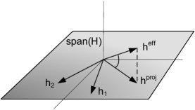
Figure 1: Quantization procedure for a two antenna mobile

IV Sum Rate Analysis

The effective channel quantization procedure converts the multiple transmit, multiple receive antenna downlink channel into a multiple transmit, single receive antenna downlink channel with channel vectors ${\bf h}^{\textrm{eff}}_{1},\ldots,{\bf h}^{\textrm{eff}}_{M}$ and channel quantizations $\hat{{\bf h}}_{i}\cdots\hat{{\bf h}}_{M}$. In fact, the transmitter need not even be aware of the number of receive antennas, since the multiple receive antennas are used only during quantization.

After receiving the quantization indices from each of the mobiles, the transmitter performs zero-forcing beamforming (as described in Section II-B) based on the channel quantizations. The resulting SINR at the $i$-th receiver is given by:

$$SINR_{i}=\frac{\frac{P}{M}|({\bf h}^{\textrm{eff}}_{i})^{H}{\bf v}_{i}|^{2}}{1+\sum_{j\neq i}\frac{P}{M}|({\bf h}^{\textrm{eff}}_{i})^{H}{\bf v}_{j}|^{2}}.$$ (11)

We are interested in the long-term average sum rate achieved in this channel, and thus the expectation of $\sum_{i=1}^{M}\log(1+SINR_{i})$. Since the beamforming vectors are chosen according to the ZFBF criterion based on the quantized channels, they satisfy $||{\bf v}_{i}||=1$ for all $i$ and $\hat{{\bf h}}_{i}{\bf v}_{j}=0$ for all $j\neq i$. Quantization error, however, leads to mismatch between the effective channels and their quantizations, and thus strictly positive interference terms (of the form $|({\bf h}^{\textrm{eff}}_{i})^{H}{\bf v}_{j}|^{2}$) in the denominator of the SINR expression.

IV-A Preliminary Calculations

In order to analyze the expected rate of such a system, the distribution of the quantization error (between ${\bf h}^{\textrm{eff}}_{i}$ and $\hat{{\bf h}}_{i}$) and of the effective channel must be characterized. Note that we consider these distributions over the randomly generated channels as well as the random vector quantization.

Lemma 1

The quantity $\cos^{2}(\angle(\hat{{\bf h}_{i}},{\bf h}^{\textrm{eff}}_{i}))$, which is one minus the quantization error $\sin^{2}(\angle(\hat{{\bf h}_{i}},{\bf h}^{\textrm{eff}}_{i}))$, is the maximum of $2^{B}$ independent beta $(N,M-N)$ random variables.

Proof:

Let ${\bf q}_{1},\ldots,{\bf q}_{N}$ represent an orthonormal basis for span$({\bf H}_{i})$. Since the quantization vectors are unit norm, $\cos^{2}\left(\angle({\bf w}_{j},\textrm{span}({\bf H}_{i})\right)=\sum_{k=1}^{N}|{\bf w}_{j}^{H}{\bf q}_{k}|^{2}$ for any quantization vector. Since the basis vectors and quantization vectors are isotropically chosen, this quantity is the squared norm of the projection of a random vector in ${\mathcal{C}}^{M}$ onto a random $N$-dimensional subspace, which is described by the beta distribution with parameters $N$ and $M-N$ [9]. Furthermore, these random variables are independent for different quantization vectors (i.e., different $j$) due to the independence of the quantization vectors and channels. ∎

Using the basic properties of the beta distribution, this implies that the quantization error which is one minus the quantization error $\sin^{2}(\angle(\hat{{\bf h}_{i}},{\bf h}^{\textrm{eff}}_{i}))$, is the minimum of $2^{B}$ independent beta $(M-N,N)$ random variables.

The following lemma and conjecture characterize the distribution of the effective channel vectors.

Lemma 2

The normalized effective channels $\frac{{\bf h}^{\textrm{eff}}_{1}}{||{\bf h}^{\textrm{eff}}_{1}||},\ldots,\frac{{\bf h}^{\textrm{eff}}_{M}}{||{\bf h}^{\textrm{eff}}_{M}||}$ are iid isotropic vectors in ${\mathcal{C}}^{M}$.

Proof:

From the earlier description of effective channel quantization, note that $\frac{{\bf h}^{\textrm{eff}}_{i}}{||{\bf h}^{\textrm{eff}}_{i}||}={\bf s}_{i}^{\textrm{proj}}$, which is the projection of the best quantization vector onto span$({\bf H}_{i})$. Since each quantization vector is chosen isotropically, its projection is isotropically distributed within the subspace. Furthermore, the best quantization vector is chosen based solely on the angle between the quantization vector and its projection. Thus ${\bf s}_{i}^{\textrm{proj}}$ is isotropically distributed in span$({\bf H}_{i})$. Since this subspace is also isotropically distributed, the vector ${\bf s}_{i}^{\textrm{proj}}$ is isotropically distributed in ${\mathcal{C}}^{M}$. To show independence, note that the quantization vectors and the channel realizations, from which the effective channel is generated, are independent from mobile to mobile. ∎

Conjecture 1

The squared norm of the effective channel ${\bf h}^{\textrm{eff}}_{i}$ is chi-squared with $2(M-N+1)$ degrees of freedom.

While this conjecture can be proven for the case when $N=M$ using the fact that the diagonal entries of $({\bf H}_{i}{\bf H}_{i}^{H})^{-1}$ are each inverted chi-square with two degrees of freedom when ${\bf H}_{i}$ is square [10, Theorem 3.2.12], this proof does not yet extend to the scenario where $1<N<M$. However, numerical results very strongly indicate that the conjecture is true for all values of $N$ and $M$. The claim is trivially true when $N=1$ because ${\bf h}^{\textrm{eff}}_{i}={\bf h}_{i}$ when mobiles have a single antenna). Furthermore, it is known that $1/({\bf v}^{H}{\bf H}_{i}^{H}{\bf H}_{i})^{-1}{\bf v})$ is chi-square distributed with $2(M-N+1)$ degrees of freedom for any unit norm ${\bf v}$ [10].

Note that if $N=M$, there is zero quantization error but the resulting effective channels have only two degrees of freedom. This scenario is not relevant, however, because higher rates can be achieved by simply transmitting to a single user using point-to-point MIMO techniques, since such a system has the same number of spatial degrees of freedom as the downlink channel. If $N<M$, the quantization error is strictly positive with probability one by the properties of the beta distribution.

IV-B Sum Rate Performance Relative to Perfect CSIT

In order to study the effect of finite rate feedback, we compare the sum rate achieved using finite rate feedback and effective channel quantization (for $N\geq 1$), denoted $R_{FB}(P)$, to the sum rate achieved with perfect CSIT in an $M$ transmit, single receive antenna downlink channel, denoted $R_{ZF}(P)$. We use the single receive antenna downlink with perfect CSIT as the benchmark instead of the $N$ receive antenna perfect CSIT downlink channel because the proposed method effectively utilizes a single receive antenna per mobile for reception, and thus cannot outperform a single receive antenna downlink channel with perfect CSIT, even in the limit of an infinite number of feedback bits. Furthermore, this analysis allows us to compare the required feedback load with $N>1$ and the proposed method to the required feedback load for downlink channels with single receive antennas, studied in [3].

Let us first analyze the rates achieved in a single receive antenna downlink channel using ZFBF under the assumption of perfect CSIT. If the transmitter has perfect CSIT, the beamforming vectors (denoted ${\bf v}_{ZF,i}$) can be chosen perfectly orthogonal to all other channels, thereby eliminating all multi-user interference. Thus, the SNR of each user is as given in (5) with zero interference terms in the denominator. The resulting average rate is given by:

$$E_{{\bf H}}[R_{ZF}(P)]=E_{{\bf H}}\left[\log\left(1+\frac{P}{M}|{\bf h}_{i}^{H}{\bf v}_{ZF,i}|^{2}\right)\right].$$

Since the beamforming vector ${\bf v}_{ZF,i}$ is chosen orthogonal to the $(M-1)$ other channel vectors $\{{\bf h}_{j}\}_{j\neq i}$, each of which is an iid isotropic vector, the beamforming vector is also an isotropic vector, independent of the channel vector ${\bf h}_{i}$. Because the effective channel vectors are isotropically distributed (Lemma 2), the same is true of the beamforming vectors and the effective channel vectors when the proposed method is used.

If the number of feedback bits is fixed, the rates achieved with finite rate feedback are bounded even as the SNR is taken to infinity. Thus, the number of feedback bits must be appropriately scaled in order to avoid this limitation. Furthermore, it is useful to consider the scaling of bits required to maintain a desired rate (or power) gap between perfect CSIT and limited feedback. Thus, we study the rate gap at asymptotically high SNR, denoted as $\Delta R$. Some simple algebra yields the following upper bound to $\Delta R$:

$$\Delta R \triangleq \lim_{P\rightarrow\infty}E_{{\bf H},W}[R_{ZF}(P)-R_{LF}(P)]$$

$$\leq \lim_{P\rightarrow\infty}E_{{\bf H}}\left[\log\left(1+\frac{P}{M}|{\bf h}_{i}^{H}{\bf v}_{ZF}|^{2}\right)\right]-$$

$$E_{{\bf H},W}\left[\log\left(1+\frac{P}{M}|({\bf h}^{\textrm{eff}}_{i})^{H}{\mathbf{v}}_{i}|^{2}\right)\right]+$$

$$E_{{\bf H},W}\left[\log\left(1+\sum_{j\neq i}\frac{P}{M}|({\bf h}^{\textrm{eff}}_{i})^{H}{\mathbf{v}}_{j}|^{2}\right)\right]$$

The difference of the first two terms, which is the rate loss due to the reduced effective channel norm (Conjecture 1), can be computed in closed form using the expectation of the log of chi-square random variables, giving a loss of $\Delta_{a}\triangleq\log_{2}e\sum_{l=M-N+1}^{M-1}\frac{1}{l}$. The final term, which is the rate loss due to the quantization error, can be upper bounded using Jensen’s inequality and some of the techniques from [3] to give:

$$\Delta R \leq \Delta_{a}+\log E_{{\bf H},W}\left[1+\sum_{j\neq i}\frac{P}{M}|({\bf h}^{\textrm{eff}}_{i})^{H}{\mathbf{v}}_{j}|^{2}\right]$$

$$= \Delta_{a}+\log\left[1\!+\!P\!\left(\frac{M\!-N\!+1}{M}\right)\!E[\sin^{2}(\angle(\hat{{\bf h}_{i}},{\bf h}^{\textrm{eff}}_{i}))]\right]$$

We now utilize Lemma 1 to estimate the quantization error. If we let $X$ be a beta$(M-N,N)$ random variable, the CCDF of $X$ can be accurately approximated for $x\approx 1$ as $\textrm{Pr}(X\geq x)\approx{M\!-\!1\choose N\!-\!1}(1-x)^{(M-N)}$. Since the quantization error is one minus the maximum of $2^{B}$ such random variables, we use extreme value theory and find $x$ such that $\textrm{Pr}(X\geq x)=2^{-B}$ to get the following approximation for the quantization error:

$$E[\sin^{2}(\angle(\hat{{\bf h}_{i}},{\bf h}^{\textrm{eff}}_{i}))]\approx 2^{-\frac{B}{M-N}}{M\!-\!1\choose N\!-\!1}^{-\frac{1}{M-N}}$$

Thus we have

$$\Delta R \approx \log_{2}e\sum_{l=M-N+1}^{M-1}\frac{1}{l}+$$

$$\log\left(1\!+\!P\cdot\left(\frac{M\!-\!N\!+\!1}{M}\right)2^{-\frac{B}{M-N}}{M\!-\!1\choose N\!-\!1}^{-\frac{1}{M-N}}\right)$$

If we set this quantity equal to a desired rate gap $r>0$ and solve for the required scaling of $B$ as a function of the SNR (in dB) we get:

$$B = \frac{M-N}{3}P_{dB}-(M-N)\log_{2}c$$

$$-(M-N)\log_{2}\left(\frac{M}{M\!-\!N\!+\!1}\right)-\log_{2}{M\!-\!1\choose N\!-\!1},$$

where $c=2^{r}\cdot e^{-(\sum_{l=M-N+1}^{M-1}\frac{1}{l})}-1$. Note that a per user rate gap of $r=1$ bps/Hz is equivalent to a 3 dB gap in the sum rate curves. If we compute the difference between this expression and the feedback load required when $N=1$ (given in (1)) and a 3 dB gap is desired ($r=1$), we can get the following approximation for the feedback reduction as a function of the number of mobile antennas $N$:

$$\Delta_{FB}(N)\approx\frac{N-1}{3}P_{dB}+\log_{2}{M\!-\!1\choose N\!-\!1}-(N-1)\log_{2}e.$$

For $N=2$, the feedback savings is given by:

$$\Delta_{FB}(2)\approx\frac{1}{3}P_{dB}+\log_{2}(M-1)-\log_{2}e.$$

The sum rate of a 6 transmit antenna downlink channel is plotted in Fig. 2. The perfect CSIT zero-forcing curve is plotted along with the rates achieved using finite rate feedback with the feedback load scaled as specified in (IV-B) for $N=1,2$ and $3$. Notice that the rates achieved for different numbers of transmit antennas are nearly indistinguishable, and all three curves are approximately 3 dB shifts of the perfect CSIT curve. In this system, the feedback savings at 20 dB is 7 and 12 bits, respectively, for $2$ and $3$ receive antennas.

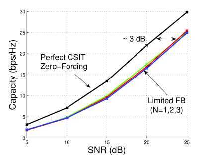
Figure 2: Sum rate of $M=K=6$ downlink channel

References

- [1] G. Caire and S. Shamai, “On the achievable throughput of a multiantenna Gaussian broadcast channel,” IEEE Trans. Inform. Theory, vol. 49, no. 7, pp. 1691–1706, July 2003.
- [2] N. Jindal and A. Goldsmith, “Dirty paper coding vs. TDMA for MIMO broadcast channels,” IEEE Trans. Inform. Theory, vol. 51, no. 5, pp. 1783–1794, May 2005.
- [3] N. Jindal, “MIMO broadcast channels with finite rate feedback,” in Proceedings of IEEE Globecom, 2005.
- [4] P. Ding, D. Love, and M. Zoltowski, “Multiple antenna broadcast channels with partial and limited feedback,” 2005, submitted to IEEE Trans. Sig. Proc.
- [5] W. Santipach and M. Honig, “Asymptotic capacity of beamforming with limited feedback,” in Proceedings of Int. Symp. Inform. Theory, July 2004, p. 290.
- [6] D. Love, R. Heath, W. Santipach, and M. Honig, “What is the value of limited feedback for MIMO channels?” IEEE Communications Magazine, vol. 42, no. 10, pp. 54–59, Oct. 2004.
- [7] D. Love, R. Heath, and T. Strohmer, “Grassmannian beamforming for multiple-input multiple-output wireless systems,” IEEE Trans. Inform. Theory, vol. 49, no. 10, pp. 2735–2747, Oct. 2003.
- [8] K. Mukkavilli, A. Sabharwal, E. Erkip, and B. Aazhang, “On beamforming with finite rate feedback in multiple-antenna systems,” IEEE Trans. Inform. Theory, vol. 49, no. 10, pp. 2562–2579, Oct. 2003.
- [9] A. K. Gupta and S. Nadarajah, Handbook of Beta Distribution and Its Applications. CRC, 2004.
- [10] R. J. Muirhead, Aspects of Multivariate Statistical Theory. Wiley, 1982.