Universal Lossless Compression with Unknown Alphabets - The Average Case

Abstract

Universal compression of patterns of sequences generated by independently identically distributed (i.i.d.) sources with unknown, possibly large, alphabets is investigated. A pattern is a sequence of indices that contains all consecutive indices in increasing order of first occurrence. If the alphabet of a source that generated a sequence is unknown, the inevitable cost of coding the unknown alphabet symbols can be exploited to create the pattern of the sequence. This pattern can in turn be compressed by itself. It is shown that if the alphabet size $k$ is essentially small, then the average minimax and maximin redundancies as well as the redundancy of every code for almost every source, when compressing a pattern, consist of at least $0.5\log\left(n/k^{3}\right)$ bits per each unknown probability parameter, and if all alphabet letters are likely to occur, there exist codes whose redundancy is at most $0.5\log\left(n/k^{2}\right)$ bits per each unknown probability parameter, where $n$ is the length of the data sequences. Otherwise, if the alphabet is large, these redundancies are essentially at least $O\left(n^{-2/3}\right)$ bits per symbol, and there exist codes that achieve redundancy of essentially $O\left(n^{-1/2}\right)$ bits per symbol. Two sub-optimal low-complexity sequential algorithms for compression of patterns are presented and their description lengths analyzed, also pointing out that the pattern average universal description length can decrease below the underlying i.i.d. entropy for large enough alphabets.

Index Terms: patterns, index sequences, universal coding, average redundancy, individual redundancy, minimax redundancy, maximin redundancy, redundancy for most sources, i.i.d. sources, MDL, redundancy-capacity theorem, sequential codes.

1 Introduction

Classical universal compression [5] usually considers coding sequences that were generated by a source with a known alphabet but with some unknown statistics. In this paper, we consider the universal coding problem, where an independently identically distributed (i.i.d.) source generates data from an alphabet that is totally unknown to both encoder and decoder, and whose size $k$ can grow with $n$. In this case, the cost of coding the alphabet letters is inevitable and depends strictly on the alphabet letters themselves. However, after coding of the alphabet letters, the data sequence can be uniquely represented by its pattern. The pattern of a sequence is a sequence of pointers that point to the actual alphabet letters, where the alphabet letters are assigned indices in order of first occurrence. For example, the pattern of the sequence “lossless” is “12331433”. A pattern sequence thus contains all positive integers from $1$ up to a maximum value $k$ in increasing order of first occurrence, and is also independent of the alphabet of the actual data. One can separate the coding of the alphabet symbols from that of the pattern, and use universal coding techniques to encode patterns. The universal coding cost of a totally unknown alphabet is inevitable regardless of the code used, and depends strictly on the actual alphabet letters. Therefore, the more interesting universal coding problem becomes that of efficiently encoding the alphabet independent patterns.

To the best of our knowledge, the idea of separating the description of the alphabet symbols from the representation of the pattern of a sequence for universal coding first appeared in the literature in [1]. This procedure was motivated in [1] by the multi-alphabet coding problem [41], i.e., the problem in which a sequence is generated by a known alphabet, but contains only a small subset of the alphabet letters. A separate description was used to inform the decoder which symbols from the alphabet have occurred in a sequence, and then their pattern was coded separately. However, no theoretical evidence was provided to show that such a technique has advantage over other multi-alphabet coding techniques, as those proposed in [41].

Stronger motivation for coding patterns of sequences was first given by Jevtić, Orlitsky, and Santhanam [13] (see also [17]-[21]), who motivated this problem by the problem of universal coding of sequences generated by sources over alphabets that are initially unknown to both the encoder and the decoder. The encoder then has to send the decoder complete information about the alphabet letters, and can utilize this inevitable cost to improve the coding performance by representing the actual data sequence by its pattern. This problem can be strongly motivated by many practical applications that compress sequences generated by either a small or a large alphabet. For example, consider transmission of text in a language that was never seen before. The graphical structure of the letters must first be transmitted. If it is transmitted in the order of first occurrence, the pattern of the text can then be compressed. This application further motivates the problem of pattern compression over large alphabets because in text the natural alphabet unit can be a word instead of a letter. Another example is compression of sequences of species first seen on another planet. Since there is no prior knowledge of their forms, they can be designated by their pattern, i.e., the first specie encountered is number $1$, the second number $2$, and so on.

The i.i.d. case is the simplest one to consider. However, coding of patterns whose underlying process is i.i.d. is different from coding of i.i.d. sequences because the constraints that are imposed by the definition of a pattern result in a non-i.i.d. probability mass function over the patterns that is different from the i.i.d. one of the original sequence. This allows shorter representations for patterns than those that would be used for the underlying i.i.d. sequences. Of course, this improvement is not free, and it only comes because of the inevitable price of representing the alphabet itself. However, while it was shown by Kieffer in [14] that if the alphabet size is very large (goes to infinity), no universal code exists, i.e., no code can achieve vanishing redundancy for i.i.d. sequences, this is not the case for the resulting patterns, as was first shown by Orlitsky et. al. in [13], [17]-[20], because only at most $n$ letters of the actual alphabet appear in the pattern sequence. Furthermore, better universal compression performance is also possible in the case where the alphabet size $k$ is sub-linear in $n$ or even fixed. Moreover, even better non-universal compression is sometimes possible because every pattern represents a collection of many sequences, thus reducing the overall pattern entropy (see, e.g., [31], [34], [36], [38], [39]).

The classical setting of the universal lossless compression problem [5] assumes that a sequence $x^{n}$ of length $n$ that was generated by a source $\theta$ is to be compressed without knowledge of the particular $\theta$ that generated $x^{n}$ but with knowledge of the class $\Lambda$ of all possible sources $\theta$. The average performance of any given code, that assigns a length function $L(\cdot)$, is judged on the basis of the redundancy function $R_{n}\left(L,\mbox{\boldmath$\theta$}\right)$, which is defined as the difference between the expected code length of $L\left(\cdot\right)$ with respect to (w.r.t.) the given source probability mass function $P_{\theta}$ and the $n$th-order entropy of $P_{\theta}$ normalized by the length $n$ of the un-coded sequence.

Naturally, the lack of knowledge of the source parameters in universal coding results in some redundancy when coding data emitted by any or almost any unknown source from a known class. To measure the universality of such a class, some notion of this redundancy is used to represent the best possible performance for some worst case, i.e., the redundancy expected from the best code for the worst case. This notion of redundancy thus serves as a lower bound on the worst case redundancy of any code for this class of sources. Two such notions are the maximin redundancy and the minimax redundancy, defined in Davisson [5]. In the maximin Bayesian approach, the parameter $\theta$ is considered random, and the maximin redundancy is obtained by the worst distribution that maximizes the minimum expected redundancy, i.e., the worst distribution for the best code. The minimax approach considers the parameter to be deterministic, and defines the minimax redundancy as the redundancy of the best code for the worst choice of $\theta$. A third stronger notion of redundancy for “most” sources in a class was later established by Rissanen [24]. This notion describes the performance of the best possible code for almost every source in the class except a subset of the class whose probability under the uniform prior (i.e., distribution in $\Lambda$) is negligible, and for which smaller redundancy can be obtained. A different approach to the study of universal codes is that of individual sequences. The minimax redundancy for individual sequences [40] is the redundancy of the best code for the worst possible sequence $x^{n}$ that can be generated by any source in the class. In this paper, however, we focus on average redundancies.

Several publications [5], [6], [7], [10], [24] investigated the average redundancy performance in standard compression of classes of parametric sources and in particular i.i.d. sources over alphabets of size $k$, which are governed by $k-1$ parameters. It was shown that for a finite size alphabet, each unknown probability parameter costs at least $0.5\log n$ extra redundancy bits. This lower bound applies in all average senses: minimax and maximin (which were demonstrated to be identical), and for almost all sources in the class. It also applies in the minimax individual sense. Furthermore, it was shown to be achievable, and in particular by using a linear complexity (fixed per symbol) sequential coding scheme that combines the universal mixture based Krichevsky-Trofimov (KT) probability estimators [15] with arithmetic coding [25]. Recently, [29], [30], [33], we extended the average results and showed that if the alphabet size is allowed to grow sub-linearly with $n$, each probability parameter costs $0.5\log(n/k)$ bits in all average senses, and also this redundancy is achievable even sequentially with the KT estimators. At the same time, related results have been independently obtained for the individual case by Orlitsky, Santhanam, and Zhang [19], [21].

While standard universal compression, in particular that of i.i.d. sources, has been extensively researched, the problem of compression of patterns has only been addressed recently, with focus, until now, only on the individual sequence case. The initial work on this problem was presented in [1]. However, Jevtić, Orlitsky, Santhanam, and Zhang [13], [17]-[21] have recently achieved significant progress in understanding this problem. In particular, they considered the performance of the best universal code for the worst sequence over all possible patterns generated by underlying i.i.d. sequences of length $n$. Using combinatoric techniques, they have shown that the minimax individual redundancy is lower bounded by $O\left(n^{-2/3}\right)$ bits per symbol and upper bounded by $O\left(n^{-1/2}\right)$ bits per symbol. They have also derived a high complexity sequential algorithm that achieves the order of the upper bound and a sub-optimal computationally heavy low complexity sequential algorithm that achieves redundancy of $O\left(n^{-1/3}\right)$ bits per symbol.

In this paper, we focus, unlike previous work, on the average redundancy performance of universal codes for coding patterns. We also consider the different behavior for different alphabet sizes $k$, and investigate the actual description length required for patterns. First, lower bounds on the average minimax/maximin redundancies are obtained as a function of the alphabet size $k$. (These bounds naturally apply also to the worst case individual redundancies.) Then, we derive lower bounds on the redundancy for most sources. Next, we obtain upper bounds on the redundancy focusing on the case in which all actual alphabet symbols are likely to be observed in the coded sequence. Although we use techniques that are much different from those used in [1], [13], [17]-[21] for the derivation of the minimax lower bound and the upper bound, the average case results we obtain in this paper demonstrate similar behavior of the redundancy in the average cases to that of the individual worst case. This is very important, because it demonstrates that the expected behavior for the worst setting is not much better than the worst sequence behavior. Hence, when coding patterns, like when coding standard sequences, one cannot expect to perform significantly better for the worst source than the performance for the worst sequence. Next, two sub-optimal low-complexity sequential algorithms are presented. The actual description length of these algorithms is studied (where the displacement relative to the i.i.d. source entropy, defined as the modified redundancy for patterns is considered). The description length for these algorithms demonstrates an interesting result, where the pattern entropy for large enough alphabets must decrease compared to the i.i.d. one. Subsequently to the work presented here (see also [36]), pattern entropy and entropy rate have been extensively studied, first in [34], and later in [11]-[12], [22]-[23], [31], [38]-[39].

To derive the lower bounds, we use the relations between redundancy and capacity that are presented in Section 3 based on [5], [9], [16]. The minimax/maximin bound we obtain for larger $k$’s is larger than that obtained for most sources. This is because we must use different techniques to derive the two bounds, where the more demanding conditions to obtain the bound for most sources result in a smaller bound. This hints to the fact that it may be possible that in the case of patterns, it may cost more redundancy beyond the entropy to code the worst source than it costs to code most other sources in the class. The upper bounds are obtained by a constructive approach. For small $k$’s it combines Rissanen’s approach [24] with our recent approach from [30], [33] and with the more demanding conditions in coding patterns.

For readability and convenience, each of the sections that contain heavy analysis is structured such that the results and their properties are described first. Then, a short description of the structure of the proof is given. Finally, each such section is concluded with the technical proofs, where steps that require much technical detail are relegated to appendices.

The outline of the paper is as follows. In Section 2, we define the notation. Section 3 reviews the individual sequence results of coding patterns, and the techniques we use to derive the new results. Section 4 summarizes the main results in the paper. Sections 5 and 6 contain the derivations of the minimax/maximin lower bounds and the bounds for most sources, respectively. In Section 7, we derive upper bounds on the redundancy with focus on the class of sources for which all symbols are likely to be observed. In Section 8, we present the sequential algorithms and study their description lengths and their displacements from the i.i.d. entropy. Then, in Section 9, a discussion about the results is presented. Finally, some concluding remarks are brought in Section 10.

2 Notation and Definitions

2.1 Universal Coding

Let $x^{n}\stackrel{{\scriptstyle\triangle}}{{=}}\left(x_{1},x_{2},\ldots,x_{n}\right)$ denote a sequence of $n$ symbols over an unknown alphabet $\Sigma$ of size $k$. The class of all i.i.d. sources that can generate any sequence $x^{n}$ over $\Sigma$ will be denoted by $\Lambda$. The subclass of i.i.d. sources that generate up to $k$ alphabet symbols will be denoted by $\Lambda_{k}$. The subclass of sources that generate $k$ symbols that are likely to be observed with probability greater than $1-o(k/n)$ will be denoted by $\tilde{\Lambda}_{k}$. A parameter $\mbox{\boldmath$\theta$}\in\Lambda_{k}$ is a vector of $k-1$ probability parameters $\mbox{\boldmath$\theta$}\stackrel{{\scriptstyle\triangle}}{{=}}\left(\theta_{1},\theta_{2},\ldots,\theta_{k-1}\right)$. For convenience, we will sometimes use the constrained component $\theta_{k}$ of $\theta$. All $k$ components of $\theta$ are non-negative and sum up to $1$. In general, boldface letters will denote vectors, whose components will be denoted by their indices in the vector. We will use hat to denote the Maximum Likelihood (ML) estimator of a parameter obtained from the data sequence $x^{n}$, e.g. $\hat{\mbox{\boldmath$\theta$}}$ will denote the ML estimator of $\theta$. Capital letters will denote random variables.

Let $\mbox{\boldmath$\theta$}\in\Lambda_{k}$ be a parameter vector that determines the statistical parameters of some source in the class $\Lambda_{k}$. Let $x^{n}$ be a sequence of $n$ symbols generated by the source $\theta$. The average $n$th-order redundancy obtained by a code that assigns length function $L(\cdot)$ for source $\theta$ is defined as

$$R_{n}\left(L,\mbox{\boldmath$\theta$}\right)\stackrel{{\scriptstyle\triangle}}{{=}}\frac{1}{n}E_{\theta}L\left[X^{n}\right]-H_{\theta}\left[X\right],$$ (1)

where $E_{\theta}$ denotes expectation w.r.t. the parameter $\theta$, and $H_{\theta}\left[X\right]$ is the (per-symbol) entropy of the source. (We will also use $H_{\theta}\left[X^{n}\right]$ as the $n$th-order sequence entropy of $\theta$, where in the i.i.d. case, $H_{\theta}\left[X^{n}\right]=nH_{\theta}\left[X\right]$.) It has been established in the literature (see, e.g., [15], [16], [24]) that assigning a universal probability $Q\left(x^{n}\right)$ is identical to designing a universal code for coding $x^{n}$, because entropy coding techniques can be used to code the sequence using a number of bits that equals, up to integer length constraints, to the negative logarithm to the base of $2$ of the assigned probability. In particular, one can use arithmetic coding [25] to allow sequential coding with sequential probability assignment schemes. We will thus ignore integer length constraints, and in places consider the redundancy as a function of the probability assignment scheme $Q\left(\cdot\right)$ instead of the code $L\left(\cdot\right)$.

We can also define the individual sequence redundancy (see, e.g., [40]) of a code with length function $L\left(\cdot\right)$ per sequence $x^{n}$ as

$$R_{n}\left(L,x^{n}\right)\stackrel{{\scriptstyle\triangle}}{{=}}\frac{1}{n}\left\{L\left(x^{n}\right)+\log P_{ML}\left(x^{n}\right)\right\},$$ (2)

where the logarithm function is taken to the base of $2$, here and elsewhere, and $P_{ML}\left(x^{n}\right)\stackrel{{\scriptstyle\triangle}}{{=}}P_{\hat{\theta}}\left(x^{n}\right)$ is the probability of $x^{n}$ given by the ML estimator $\hat{\mbox{\boldmath$\theta$}}$ of the governing parameters. The negative logarithm of this probability is the smallest possible code length for a particular sequence under a given statistical model (in our case the i.i.d. one).

The average minimax redundancy of the class $\Lambda_{k}$ is defined as

$$R_{n}^{+}\left(\Lambda_{k}\right)\stackrel{{\scriptstyle\triangle}}{{=}}\min_{L}\sup_{\mbox{\boldmath$\theta$}\in\Lambda_{k}}R_{n}\left(L,\mbox{\boldmath$\theta$}\right).$$ (3)

Similarly, we can define the individual minimax redundancy as that of the best code $L\left(\cdot\right)$ for the worst sequence $x^{n}$, i.e.,

$$\hat{R}_{n}^{+}\left(\Lambda_{k}\right)\stackrel{{\scriptstyle\triangle}}{{=}}\min_{L}\sup_{\mbox{\boldmath$\theta$}\in\Lambda_{k}}\max_{x^{n}}\frac{1}{n}\left\{L\left(x^{n}\right)+\log P_{\theta}\left(x^{n}\right)\right\}.$$ (4)

To define the maximin redundancy of $\Lambda_{k}$, let us assign a probability measure (prior) $w\left(\cdot\right)$ on $\Lambda_{k}$ and let us define the mixture source

$$P_{w}\left(x^{n}\right)\stackrel{{\scriptstyle\triangle}}{{=}}\int_{\Lambda_{k}}w\left(d\mbox{\boldmath$\theta$}\right)P_{\theta}\left(x^{n}\right).$$ (5)

The average redundancy associated with a length function $L\left(\cdot\right)$ is defined as

$$R_{n}\left(L,w\right)\stackrel{{\scriptstyle\triangle}}{{=}}\int_{\Lambda_{k}}w\left(d\mbox{\boldmath$\theta$}\right)R_{n}\left(L,\mbox{\boldmath$\theta$}\right).$$ (6)

The minimum expected redundancy for a given prior $w$ (which is attained by the ideal code length w.r.t. the mixture, $L\left(x^{n}\right)=-\log P_{w}\left(x^{n}\right)$) is defined as

$$R_{n}\left(w\right)\stackrel{{\scriptstyle\triangle}}{{=}}\min_{L}R_{n}\left(L,w\right).$$ (7)

Finally, the maximin redundancy of the class $\Lambda_{k}$ is the worst case minimum expected redundancy among all priors $w$, i.e.,

$$R_{n}^{-}\left(\Lambda_{k}\right)\stackrel{{\scriptstyle\triangle}}{{=}}\sup_{w}R_{n}\left(w\right).$$ (8)

2.2 Patterns

The pattern of a sequence $x^{n}$ will be denoted by $\Psi\left(x^{n}\right)$. Many different sequences over the same alphabet (and over different alphabets) have the same pattern. For example, for the sequences $x^{n}=$“lossless”, $x^{n}=$“sellsoll”, $x^{n}=$“12331433”, and $x^{n}=$“76887288”, the pattern is $\Psi\left(x^{n}\right)=$“12331433”. Therefore, for given $\Sigma$ and $\theta$, the probability of a pattern induced by an i.i.d. underlying probability is given by

$$P_{\theta}\left[\Psi\left(x^{n}\right)\right]=\sum_{y^{n}:\Psi(y^{n})=\Psi(x^{n})}P_{\theta}\left(y^{n}\right).$$ (9)

We note that the probability in (9) is dominated by some of the sequences, where others only contribute negligibly. This fact is used to derive an upper bound in Section 7. The per sequence (block) pattern entropy of order $n$ of a source $\theta$ is thus defined as

$$H_{\theta}\left[\Psi\left(X^{n}\right)\right]\stackrel{{\scriptstyle\triangle}}{{=}}-\sum_{\Psi\left(x^{n}\right)}P_{\theta}\left[\Psi\left(x^{n}\right)\right]\log P_{\theta}\left[\Psi\left(x^{n}\right)\right].$$ (10)

In order to define the redundancy function of patterns for a given code and a given source $\theta$, we need to realize that a vector $\mbox{\boldmath$\theta$}^{\prime}$ that is a permutation of another vector $\theta$ produces similar typical patterns, and is, in fact, the same source in the pattern domain. Therefore, we can define the notation $\mbox{\boldmath$\psi$}\left(\mbox{\boldmath$\theta$}\right)$ as the permutation of $\theta$ which is ordered in non-decreasing order of components, i.e., $\psi_{1}\left(\mbox{\boldmath$\theta$}\right)\leq\psi_{2}\left(\mbox{\boldmath$\theta$}\right)\leq\ldots\leq\psi_{k}\left(\mbox{\boldmath$\theta$}\right)$. For example, if $\mbox{\boldmath$\theta$}=\left(0.7,0.1,0.2\right)$, then $\mbox{\boldmath$\psi$}\left(\mbox{\boldmath$\theta$}\right)=\left(0.1,0.2,0.7\right)$. We can also, alternately, view a vector $\sigma$ as a permutation vector of indices, and use $\theta\left(\sigma_{i}\right)$ to denote the $i$th component of the permuted vector $\theta$, permuted according to $\sigma$. For the example above, if we define $\mbox{\boldmath$\sigma$}=\left(3,1,2\right)$, then $\mbox{\boldmath$\theta$}\left(\mbox{\boldmath$\sigma$}\right)=\left(0.2,0.7,0.1\right)$ and $\theta\left(\sigma_{2}\right)=\theta_{1}=0.7$. In most sections, we will consider the original vector $\theta$ to be already ordered non-decreasingly, and therefore the identity permutation $\mbox{\boldmath$\sigma$}=\left(1,2,\ldots,k\right)$ will give $\mbox{\boldmath$\psi$}\left(\mbox{\boldmath$\theta$}\right)=\mbox{\boldmath$\theta$}=\mbox{\boldmath$\theta$}\left(\mbox{\boldmath$\sigma$}\right)$. All vectors $\mbox{\boldmath$\psi$}\left(\mbox{\boldmath$\theta$}\right)$ for all $\mbox{\boldmath$\theta$}\in\Lambda_{k}$ will constitute the pattern space $\Psi\left(\Lambda_{k}\right)$, and similarly, we can define $\Psi\left(\Lambda\right)$ as the pattern space induced by (or projected from) the class $\Lambda$.

The average pattern redundancy for coding patterns generated by a source $\theta$ using a code that assigns a representation of length $L\left[\Psi\left(x^{n}\right)\right]$ to the pattern of sequence $x^{n}$ is defined as

$$R_{n}\left[L,\mbox{\boldmath$\psi$}\left(\mbox{\boldmath$\theta$}\right)\right]\stackrel{{\scriptstyle\triangle}}{{=}}\frac{1}{n}E_{\theta}L\left[\Psi\left(X^{n}\right)\right]-\frac{1}{n}H_{\theta}\left[\Psi\left(X^{n}\right)\right].$$ (11)

Similarly to (2), we can define the individual pattern redundancy for a given code as

$$R_{n}\left[L,\Psi\left(x^{n}\right)\right]\stackrel{{\scriptstyle\triangle}}{{=}}\frac{1}{n}\left\{L\left[\Psi\left(x^{n}\right)\right]+\max_{\mbox{\boldmath$\theta$}}\left\{\log P_{\theta}\left[\Psi\left(x^{n}\right)\right]\right\}\right\}.$$ (12)

Note that the ML probability is now different from that for the simple i.i.d. case, because the ML is taken over the pattern probability and not over the i.i.d. one.

Even in the simplest i.i.d. underlying case, it becomes very difficult to derive closed form expressions beyond (9) on the probability of a pattern, (except for very specific patterns). It will therefore be useful to define quantities that relate a code length to the i.i.d. entropy in the average case and to the i.i.d. ML probability in the individual case. We will refer to these quantities as the modified redundancies. The modified redundancy will be studied in Section 8, as part of the study of the description length of the proposed sequential schemes. The average modified redundancy for a code $L\left(\cdot\right)$ that codes patterns of a source $\theta$ is defined as

$$\tilde{R}_{n}\left[L,\mbox{\boldmath$\psi$}\left(\mbox{\boldmath$\theta$}\right)\right]\stackrel{{\scriptstyle\triangle}}{{=}}\frac{1}{n}E_{\theta}L\left[\Psi\left(X^{n}\right)\right]-H_{\theta}\left[X\right].$$ (13)

The individual pattern modified redundancy is defined as

$$\tilde{R}_{n}\left[L,\Psi\left(x^{n}\right)\right]\stackrel{{\scriptstyle\triangle}}{{=}}\frac{1}{n}\left\{L\left[\Psi\left(x^{n}\right)\right]+\max_{\mbox{\boldmath$\theta$}}\left\{\log P_{\theta}\left[x^{n}\right]\right\}\right\}.$$ (14)

We should note that unlike the regular redundancy, the modified redundancy does not actually satisfy conditions that must be satisfied by redundancy functions. In particular, it can be negative also in the average case. If this happens, it simply means that one can universally describe patterns using shorter descriptions than the entropy of the underlying i.i.d. source. We will see this phenomenon in Section 8 and in [31]. The modified redundancy thus becomes handy for bounding the description length a code can assign to a pattern, i.e,

$$E_{\theta}L\left[\Psi\left(X^{n}\right)\right]=H_{\theta}\left[\Psi\left(X^{n}\right)\right]+nR_{n}\left[L,\mbox{\boldmath$\psi$}\left(\mbox{\boldmath$\theta$}\right)\right]=H_{\theta}\left[X^{n}\right]+n\tilde{R}_{n}\left[L,\mbox{\boldmath$\psi$}\left(\mbox{\boldmath$\theta$}\right)\right],$$ (15)

and we can use either equalities to bound this description length.

Using the definition of the average pattern redundancy in (11), we can replace $R_{n}\left(L,\mbox{\boldmath$\theta$}\right)$ by $R_{n}\left[L,\mbox{\boldmath$\psi$}\left(\mbox{\boldmath$\theta$}\right)\right]$ in (3) to define the average minimax pattern redundancy $R_{n}^{+}\left[\Psi\left(\Lambda_{k}\right)\right]$. Similarly, we can define the average maximin pattern redundancy $R_{n}^{-}\left[\Psi\left(\Lambda_{k}\right)\right]$ by the same substitution in (6). Taking the maximum of (12) on $x^{n}$ and the minimum on $L\left(\cdot\right)$, similarly to (4), we obtain the individual minimax pattern redundancy $\hat{R}_{n}^{+}\left[\Psi\left(\Lambda_{k}\right)\right]$. Note that all these redundancies can also be obtained w.r.t. the class of all i.i.d. sources $\Lambda$ regardless of the alphabet size. Naturally, $R_{n}^{+}\left[\Psi\left(\Lambda\right)\right]$, $R_{n}^{-}\left[\Psi\left(\Lambda\right)\right]$, and $\hat{R}_{n}^{+}\left[\Psi\left(\Lambda\right)\right]$ will take the maximal redundancy value over all alphabet sizes $k$.

3 Technical Background

3.1 Individual Pattern Redundancy

To the best of our knowledge, universal compression of patterns was first introduced by Åberg, Shtarkov and Smeets [1]. Åberg et. al. addressed the compression problem of individual pattern sequences. In particular, they used the individual sequence minimax approach developed by Shtarkov [40] to design the best code in the individual minimax sense. For standard sequence compression, this approach assigns to an $n$-symbols sequence $x^{n}$ probability $Q\left(x^{n}\right)$ that equals its ML probability normalized by the sum of the ML probabilities over all possible sequences, i.e.,

$$Q\left(x^{n}\right)\stackrel{{\scriptstyle\triangle}}{{=}}\frac{P_{ML}\left(x^{n}\right)}{\sum_{y^{n}}P_{ML}\left(y^{n}\right)},$$ (16)

where $P_{ML}\left(x^{n}\right)$ is the ML probability of $x^{n}$, and the summation is over all possible sequences $y^{n}$ of length $n$. This approach guarantees (under negligible integer length constraints) individual redundancy of

$$R_{n}\left(Q,x^{n}\right)=\frac{1}{n}\log\frac{P_{ML}\left(x^{n}\right)}{Q\left(x^{n}\right)}=\frac{1}{n}\log\left\{\sum_{y^{n}}P_{ML}\left(y^{n}\right)\right\}$$ (17)

for every sequence $x^{n}$. Equation (17) is true in particular for the worst sequence $x^{n}$ for which this redundancy is the minimal attainable. Therefore, this approach achieves the minimax redundancy.

The approach above was modified for patterns by modifying (16) to

$$Q\left[\Psi\left(x^{n}\right)\right]\stackrel{{\scriptstyle\triangle}}{{=}}\frac{P_{\widehat{\psi\left(\theta\right)}}\left[\Psi\left(x^{n}\right)\right]}{\sum_{\Psi\left(y^{n}\right):\theta\in\Psi\left(\Lambda_{k}\right)}P_{\widehat{\psi\left(\theta\right)}}\left[\Psi\left(y^{n}\right)\right]},$$ (18)

where $P_{\widehat{\psi\left(\theta\right)}}\left[\Psi\left(x^{n}\right)\right]$ is the ML pattern probability for the pattern of the sequence $x^{n}$, and the normalization factor is the sum of all ML probabilities for all possible patterns of sequences generated by sources $\mbox{\boldmath$\theta$}\in\Lambda_{k}$. Restricting the derivation to $\Lambda_{k}$ (and not the wider i.i.d. class $\Lambda$), it was shown in [1] that the normalizing sum is approximately lower bounded by

$$\sum_{\Psi\left(y^{n}\right):\theta\in\Psi\left(\Lambda_{k}\right)}P_{\widehat{\psi\left(\theta\right)}}\left[\Psi\left(y^{n}\right)\right]\gtrsim\frac{1}{k!}\cdot\frac{\sqrt{\pi}}{\Gamma\left(k/2\right)}\cdot\left(n/2\right)^{(k-1)/2},$$ (19)

where $\Gamma\left(\cdot\right)$ is the Gamma function. If further analysis steps are performed beyond those in [1], this yields a lower bound on the individual minimax pattern redundancy for patterns with at most $k$ different alphabet symbols of

$$\hat{R}_{n}^{+}\left[\Psi\left(\Lambda_{k}\right)\right]\gtrsim\left(1-\varepsilon\right)\frac{(k-1)}{2n}\log\frac{n}{k^{3}},$$ (20)

where $\varepsilon>0$ can be made arbitrarily small. This bound is, of course, useful only for $k=o\left(n^{1/3}\right)$ and becomes negative for larger alphabet sizes. Based on this result and prior results in [41], Åberg et. al. also proposed a sequential scheme for coding patterns, for which they provided empirical results. The computational requirements of this scheme appear to be rather demanding.

Major progress in the research of individual pattern compression has been recently obtained by Jevtić, Orlitsky, Santhanam, and Zhang [13], [17]-[20]. The approach used in those papers was similar to that in [1] based on Shtarkov’s minimax results and on combinatoric techniques. These papers considered the compression of patterns generated by any source from the whole class $\Lambda$, independently of the alphabet size $k$, i.e., the maximum number of different indices in the pattern. First, it was shown [13] that probability assignment of

$$\tilde{Q}\left[\Psi\left(x^{n}\right)\right]\stackrel{{\scriptstyle\triangle}}{{=}}\frac{P_{ML}\left(x^{n}\right)}{\sum_{\Psi\left(y^{n}\right):\theta\in\Psi\left(\Lambda\right)}P_{ML}\left(y^{n}\right)},$$ (21)

where $P_{ML}\left(x^{n}\right)$ is the i.i.d. ML probability (not the pattern ML probability) but the summation is only on all possible patterns, results in modified individual redundancy of

$$\tilde{R}_{n}\left[\tilde{Q},\Psi\left(x^{n}\right)\right]=\frac{1.5\log e}{n^{2/3}}+o\left(\frac{1}{n^{2/3}}\right).$$ (22)

This redundancy is obtained for every pattern of length $n$ independently of the number of indices in the pattern, and is also the minimax modified individual pattern redundancy. Then, Orlitsky et. al. [17]-[20] demonstrated that this modified redundancy is, in fact, a lower bound on the actual pattern redundancy. (Note that if the analysis in [1] is modified to the whole class $\Lambda$, one can obtain the same bound.) Using integer partitioning of a sequence of length $n$, it was also shown in [17]-[20] that there exist codes that achieve individual minimax pattern redundancy of at most $O\left(n^{-0.5}\right)$. Summarizing all these results, it was shown that there exist codes for which

$$\frac{1.5\log e}{n^{2/3}}+o\left(\frac{1}{n^{2/3}}\right)\leq\hat{R}_{n}^{+}\left[\Psi\left(\Lambda\right)\right]\leq\frac{\pi\sqrt{2/3}\log e}{\sqrt{n}}.$$ (23)

Finally, a computationally demanding high complexity sequential scheme was shown in [18]-[20] to achieve the order of the upper bound in (23), as well as a low-complexity sequential scheme that achieves minimax individual redundancy of $O\left(n^{-1/3}\right)$.

3.2 Average Case - Background

Unlike the prior results on compression of patterns, we focus on the average case problem in compression of patterns induced by sequences generated by i.i.d. sources. To derive lower and upper bounds, we will use techniques that are based on Davisson’s [5] and Rissanen’s [24] approaches, and their extension [9], [16]. In particular, the well established connection between universal coding redundancy and channel capacity will be used to obtain lower bounds on the average pattern redundancy. In [5], it was established that the maximin redundancy of a class $\Lambda_{k}$ is bounded from below by (and asymptotically equals to) the normalized capacity of the “channel” defined by the conditional probability $P_{\theta}\left(x^{n}\right)$, i.e., the channel whose input is the parameter $\theta$ and whose output is the data sequence $x^{n}$. It was further established that the average minimax redundancy is lower bounded by the maximin redundancy. Using Gallager’s later result [10] that shows that the minimax and maximin redundancies are essentially equivalent, this leads to the bound on both minimax and maximin redundancies of

$$R_{n}^{+}\left(\Lambda_{k}\right)=R_{n}^{-}\left(\Lambda_{k}\right)\geq\sup_{w}\frac{1}{n}I_{w}\left({\mathbf{\Theta}};~{}X^{n}\right),$$ (24)

where $I_{w}\left({\mathbf{\Theta}};~{}X^{n}\right)$ is the mutual information induced by the joint measure $w\left(\mbox{\boldmath$\theta$}\right)\cdot P_{\theta}\left(x^{n}\right)$. Using (24), any lower bound on the capacity of the channel defined by $P_{\theta}\left(x^{n}\right)$ can be used to bound the minimax and maximin redundancies. In particular, one can pick a set $\Omega$ of $M$ points $\mbox{\boldmath$\theta$}\in\Lambda_{k}$. If these points can be shown to be distinguishable by the sequence $X^{n}$, then $(\log M)/n$ can serve as a lower bound on the normalized capacity of the respective channel, and thus on the minimax and maximin redundancies. This lower bound is specifically implied by Fano’s Inequality using the fact that the error probability goes to $0$ (see, e.g., [16]). Distinguishability in a set of points $\Omega$ is defined (in a stronger sense than needed to the result above) as follows. Let $\mbox{\boldmath$\theta$}\in\mbox{\boldmath$\Omega$}$ be a point that generates the random sequence $X^{n}$. Let $\hat{\mbox{\boldmath$\theta$}}=f\left(X^{n}\right)$ be an estimator of $\theta$ from $X^{n}$, and let $\hat{\mbox{\boldmath$\theta$}}_{\Omega}=g\left(\hat{\mbox{\boldmath$\theta$}}\right)$ be a point in $\Omega$ that is used to estimate $\theta$ from the estimator $\hat{\mbox{\boldmath$\theta$}}$, where $\hat{\mbox{\boldmath$\theta$}}$ is not necessarily a point in $\Omega$. Then, there exist functions $f(\cdot)$ and $g(\cdot)$, such that $P_{\theta}\left(\hat{\mbox{\boldmath$\theta$}}_{\Omega}\neq\mbox{\boldmath$\theta$}\right)\rightarrow 0$ as $n\rightarrow\infty$, for every $\mbox{\boldmath$\theta$}\in\mbox{\boldmath$\Omega$}$. In words, there exists an estimator of $\theta$ out of the points in $\Omega$, such that the probability that a sequence that was generated by one point in the set would appear to have been generated by a different point in the set vanishes with $n$.

The approach described above will be adopted to patterns in order to derive the bound in Section 5. In the patterns case, we will consider the set of sources $\mbox{\boldmath$\theta$}\in\Psi\left(\mbox{\boldmath$\Omega$}\right)$, and the pattern source estimator $\mbox{\boldmath$\psi$}\left(\hat{\mbox{\boldmath$\theta$}}\right)$ will be defined as a function of the pattern, i.e., $\mbox{\boldmath$\psi$}\left(\hat{\mbox{\boldmath$\theta$}}\right)=f\left[\Psi\left(X^{n}\right)\right]$, since the sequence itself is not observed. Then, the estimator $\hat{\mbox{\boldmath$\theta$}}^{\psi}_{\Omega}=g\left[\mbox{\boldmath$\psi$}\left(\hat{\mbox{\boldmath$\theta$}}\right)\right]$ must be in the pattern source space $\Psi\left(\mbox{\boldmath$\Omega$}\right)$. Since the minimax and maximin average redundancies are essentially the same, we will consider only the minimax one, and the results will apply to both.

Merhav and Feder [16] extended the concept of the redundancy-capacity and derived a strong version of the redundancy-capacity theorem. They showed that if it is possible to partition the class $\Lambda_{k}$ into disjoint sets of sources $\theta$, each of at least $M$ points that are distinguishable by $X^{n}$, then the redundancy is lower bounded by

$$R_{n}\left(L,\mbox{\boldmath$\theta$}\right)\geq\left(1-\varepsilon\right)\frac{\log M}{n},$$ (25)

for every code $L\left(\cdot\right)$, and almost every $\mbox{\boldmath$\theta$}\in\Lambda_{k}$, where $\varepsilon>0$ is arbitrarily small. In order to be able to use this result, one needs to make sure that the points in each set are uniformly distributed within the set, and every point in $\Lambda_{k}$ is included in one set (see also [27]-[29]). Sometimes such an assumption cannot be made unless a non-uniform prior is assumed within the class. In such cases the result in (25) does not apply to most sources in the class, but to all sources in the class except a subset whose probability under the prior assumed vanishes. The technique that will be presented in Section 5 for patterns will suffer from this problem, and thus cannot be used to obtain a lower bound on the redundancy of most sources. Therefore, a different technique that uses Merhav and Feder’s theorem will be applied in Section 6 to derive a lower bound for most sources. As in Section 5, the ideas described in this paragraph for standard compression will be applied to patterns in a similar manner to that described in the preceding paragraph.

Both versions of the redundancy-capacity theorem presented above can be used by taking grids of points from the class $\Lambda_{k}$, and showing that the points in each grid are distinguishable. Then, the normalized logarithm of the number of grid points gives a lower bound on the required redundancy. For the minimax redundancy, one such grid is sufficient using the weak version of the theorem. For the redundancy for most sources, we need to show how we shift the grid to cover the whole class without violating the conditions of the strong version of the redundancy-capacity theorem, where the points in each shift of the grid remain distinguishable. For standard compression with fixed alphabet size $k$, a uniform grid with spacing of $n^{-0.5(1-\varepsilon)}$ for an arbitrarily small $\varepsilon>0$ is sufficient for distinguishability. This yields the well known bound, for which the cost of each unknown probability parameter is $0.5\log n$ bits. Recently, we showed [30], [33] that in the case of large alphabets, the simple grid used to achieve the fixed $k$ bound is not sufficient. In the minimax case, a non-uniform grid with increasing spacing in each dimension was created, and resulted in a cost of $0.5\log(n/k)$ bits for each unknown probability parameter. The same cost with smaller second order term resulted for most sources using sphere packing [2] considerations to create a grid (or lattice) of distinguishable points. (Note that this idea is in line with Rissanen’s proof for a parametric source with a finite number of parameters [24].) The ideas that led to these bounds will be modified in Sections 5 and 6 for lower bounding the minimax and most sources redundancies of patterns.

In [9], Feder and Merhav showed that there exist classes that consist of different subclasses, each with different redundancy within itself. For example, a union of subclasses $\Lambda_{k}$ constitute the class $\Lambda$. If all the subclasses are coded as one class, the redundancy adapts to the worst one among the subclasses even if the actual source is from a subclass within which smaller redundancy can be obtained. However, in most simple cases, the cost of distinguishing between subclasses is negligible w.r.t. the universal cost within each subclass. Hierarchical coding first distinguishes between the different subclasses and then between sources within each subclass. For example, if the class $\Lambda$ is considered, the encoder will first code the alphabet size $k$ and then perform universal coding within the subclass $\Lambda_{k}$. Such an approach yields lower costs for coding sources in many subclasses than the cost of coding the whole class. Therefore, unlike the results in [13], [17]-[20], we will consider the subclass $\Psi\left(\Lambda_{k}\right)$ and analyze the pattern redundancy for each $k$. If $k$ is initially unknown, $\left(1+\varepsilon\right)\log k$ bits can be used to relay to the decoder the number of indices in the pattern using Elias’s [8] coding of the integers.

One technique that will be used in Section 7 to design a code for coding patterns will use ideas as in Rissanen’s quantization two-part code method [24]. This technique estimates the ML parameters from the sequence $X^{n}$ and then quantizes them onto a grid of points. Then, only the quantized version of the ML parameters is relayed to the decoder, and entropy coding is used w.r.t. this version as if the quantized parameters are the true source parameters. The redundancy of this code consists of the cost of relaying the quantized ML estimators and the cost caused by the quantization of the ML parameters. The latter results from the deviation of the quantized parameters from the actual parameters. Usually, the quantization cost can be made negligible by tuning the grid spacing properly. Unlike Rissanen’s approach, we will need to use a non-uniform grid for the quantization, as in [30], [33], although, unlike these references, we will be concerned with index probabilities for patterns and not the actual letter probabilities.

4 The Main Results

The paper contains the following main results:

• a lower bound on the maximin and minimax redundancy for universal coding of patterns,

• a lower bound on the redundancy for most sources when coding patterns,

• an upper bound on the redundancy of coding patterns, specifically for not very large alphabets where all alphabet letters are likely to occur in a sequence,

• two sub-optimal sequential low-complexity methods for coding patterns with upper bounds on the displacements of their description lengths from the i.i.d. ML description length and also with implications to the pattern entropy.

Each of the above results is studied in a separate subsequent section.

In particular, we show that the $n$th-order maximin and minimax average universal coding redundancies for patterns induced by i.i.d. sources with alphabet size $k$ are lower bounded by

$$R^{+}_{n}\left[\Psi\left(\Lambda_{k}\right)\right]\geq\left\{\begin{array}[]{ll}\frac{k-1}{2n}\log\frac{n^{1-\varepsilon}}{k^{3}}+\frac{k-1}{2n}\log\frac{\pi e^{3}}{2}-O\left(\frac{\log k}{n}\right),&\mbox{for }k\leq\left(\frac{\pi n^{1-\varepsilon}}{2}\right)^{1/3}\\ \left(\frac{\pi}{2}\right)^{1/3}\cdot(1.5\log e)\cdot n^{-(2+\varepsilon)/3}-O\left(\frac{\log n}{n}\right),&\mbox{for }k>\left(\frac{\pi n^{1-\varepsilon}}{2}\right)^{1/3}\end{array}\right..$$ (26)

The $n$th-order average universal coding redundancy is lower bounded by

$$R_{n}\left[L,\mbox{\boldmath$\psi$}\left(\mbox{\boldmath$\theta$}\right)\right]\geq\left\{\begin{array}[]{ll}\frac{k-1}{2n}\log\frac{n^{1-\varepsilon}}{k^{3}}-\frac{k-1}{2n}\log\frac{8\pi}{e^{3}}-O\left(\frac{\log k}{n}\right),&\mbox{for }k\leq\frac{1}{2}\cdot\left(\frac{n^{1-\varepsilon}}{\pi}\right)^{1/3}\\ \frac{1.5\log e}{2\pi^{1/3}}\cdot n^{-(2+\varepsilon)/3}-O\left(\frac{\log n}{n}\right),&\mbox{for }k>\frac{1}{2}\cdot\left(\frac{n^{1-\varepsilon}}{\pi}\right)^{1/3}\end{array}\right.$$ (27)

for every code $L(\cdot)$ and almost every i.i.d. source $\mbox{\boldmath$\theta$}\in\Lambda_{k}$. Both lower bounds demonstrate that for small $k$, each parameter costs at least $0.5\log\left(n/k^{3}\right)$ bits. For larger alphabets, the cost is at least $O\left(n^{(1-\varepsilon)/3}\right)$ bits overall.

Next, it is shown that there exist codes with length function $L^{*}\left(\cdot\right)$ that achieve redundancy

$$R_{n}\left[L^{*},\mbox{\boldmath$\psi$}\left(\mbox{\boldmath$\theta$}\right)\right]\leq\left\{\begin{array}[]{ll}\left(1+\varepsilon\right)\frac{k-1}{2n}\log\frac{n^{1+\varepsilon}}{k^{2}},&\mbox{for }k\leq\sqrt{n}^{1-\varepsilon}~{}\mbox{and}~{}\mbox{\boldmath$\theta$}\in\tilde{\Lambda}_{k}\\ \frac{\pi\sqrt{2/3}\log e}{\sqrt{n}}+O\left(\frac{1}{n}\right),&\mbox{for }k\geq\sqrt{n}^{1-\varepsilon}~{}\mbox{or}~{}\mbox{\boldmath$\theta$}\not\in\tilde{\Lambda}_{k}\end{array}\right.$$ (28)

for patterns induced by any i.i.d. source $\mbox{\boldmath$\theta$}\in\Lambda_{k}$. Namely, for small $k$, each parameter costs at most $0.5\log\left(n/k^{2}\right)$ bits, and for large $k$, $O\left(\sqrt{n}\right)$ overall.

Next, a linear (per sequence) complexity sequential method (with prior knowledge of $k$) is shown with modified individual redundancy that satisfies

$$\tilde{R}_{n}\left[Q_{k},\Psi\left(x^{n}\right)\right]\leq\frac{k}{2n}\log\frac{n}{k^{3}}+\left(\frac{19}{12}\log e\right)\frac{k}{n}-\frac{1}{2n}\log n+O\left(\frac{k^{2}}{n^{2}}\right).$$ (29)

for every pattern $\Psi\left(x^{n}\right)$ of a sequence $x^{n}$ with $k$ distinct indices and for every $k\leq n$. With increased complexity, identical performance is also achieved without prior knowledge of $k$. However, a second linear complexity scheme achieves similar asymptotic performance in $k$, with only second order penalty without prior knowledge of $k$. Finally, the implications of these bounds on the pattern entropy are noticed, in particular, indicating that the pattern entropy must decrease from the i.i.d. one if $k$ is larger than $cn^{1/3}$, for some constant $c$.

5 A Maximin and Minimax Lower Bound

In [30], [32]-[33], it was established that for a large known alphabet of size $k$, choosing a set $\Omega$ of $M$ sources $\theta$ whose $k-1$ free components are placed only at points on a non-uniform grid of increased spacing in each dimension yields a set of distinguishable sources if the grid spacing is properly chosen. The $k-1$ components of grid points take values only from the grid vector $\mbox{\boldmath$\tau$}\stackrel{{\scriptstyle\triangle}}{{=}}\left(\tau_{1},\tau_{2},\ldots,\tau_{b},\ldots,\tau_{B}\right)$. The components of $\tau$ satisfy $\tau_{1}<\tau_{2}<\cdots<\tau_{b}<\cdots<\tau_{B}$, and the spacing between every two consecutive components increases with $b$. The advantage of such a grid is that it yields a tighter bound on the redundancy, as we can include more points in regions of $\Lambda_{k}$ in which closer points are distinguishable, i.e., for small probability parameters. For coding patterns, we can build a similar grid of sources. However, we need to verify distinguishability in the pattern domain, as explained in Section 3. A valid grid point $\mbox{\boldmath$\theta$}\in\mbox{\boldmath$\Omega$}$ and a non-identity permutation $\mbox{\boldmath$\theta$}^{\prime}=\mbox{\boldmath$\theta$}\left(\mbox{\boldmath$\sigma$}\right)\neq\mbox{\boldmath$\theta$}$, $\mbox{\boldmath$\theta$}^{\prime}\in\mbox{\boldmath$\Omega$}$, of $\theta$ will not be distinguishable in the pattern domain, as they are likely to generate similar patterns. Hence, in order to build a grid of sources which are distinguishable in the pattern domain, we can take the grid $\Omega$ for i.i.d. sources, but keep only one point for each set of permutations of the same source vector $\mbox{\boldmath$\theta$}\stackrel{{\scriptstyle\triangle}}{{=}}\mbox{\boldmath$\psi$}\left(\mbox{\boldmath$\theta$}\right)$ (which is ordered in non-decreasing order of components). We then consider a new grid $\Psi\left(\mbox{\boldmath$\Omega$}\right)$ that contains only points $\mbox{\boldmath$\theta$}\stackrel{{\scriptstyle\triangle}}{{=}}\mbox{\boldmath$\psi$}\left(\mbox{\boldmath$\theta$}\right)$ in which the components are ordered in nondecreasing order. In this section, we will show how such a grid can be obtained, and then will use the weak-version of the redundancy-capacity theorem to derive a lower bound on the minimax redundancy using this grid. We start by stating the main result that lower bounds the minimax pattern redundancy, and then present its proof .

Theorem 1

Fix an arbitrarily small $\varepsilon>0$, and let $n\rightarrow\infty$. Then, the $n$th-order maximin and minimax average universal coding redundancies for patterns induced by i.i.d. sources with alphabet size $k$ are lower bounded by

$$R^{+}_{n}\left[\Psi\left(\Lambda_{k}\right)\right]\geq\left\{\begin{array}[]{ll}\frac{k-1}{2n}\log\frac{n^{1-\varepsilon}}{k^{3}}+\frac{k-1}{2n}\log\frac{\pi e^{3}}{2}-O\left(\frac{\log k}{n}\right),&\mbox{for }k\leq\left(\frac{\pi n^{1-\varepsilon}}{2}\right)^{1/3}\\ \left(\frac{\pi}{2}\right)^{1/3}\cdot(1.5\log e)\cdot n^{-(2+\varepsilon)/3}-O\left(\frac{\log n}{n}\right),&\mbox{for }k>\left(\frac{\pi n^{1-\varepsilon}}{2}\right)^{1/3}\end{array}\right..$$ (30)

Theorem 1 shows that as long as $k$ is small (of $o\left(n^{1/3}\right)$), each index probability parameter costs at least $0.5\log\left(n/k^{3}\right)$ extra code bits. However, if the alphabet size is larger, a threshold phenomenon occurs, and the redundancy is of $O\left(n^{-2/3}\right)$ overall. Note that this result applies even if $k>n$, because regardless of the actual alphabet size, the number of indices that will occur in a pattern is upper bounded by $n$. The bound in the first region coincides with the individual minimax bound obtained from [1], described in (20). The second region points to the same behavior as the worst case bound in (23). The average lower bound naturally applies to the individual minimax worst case redundancy, but not the other way around. Theorem 1 shows that we are unlikely to gain much in the average case over the worst sequence at least for the minimax redundancy. The $n^{-\varepsilon/3}$ gap may indicate a true small gap between the individual worst case and the average worst case, but may also be due to sub-optimal bounding.

The proof of Theorem 1 builds a non-uniform grid $\Omega$ of points as in the i.i.d. minimax case. Then, the grid size is reduced by a factor of $k!$ eliminating all permutations of any grid point $\theta$ except the ordered permutation $\mbox{\boldmath$\psi$}\left(\mbox{\boldmath$\theta$}\right)$, resulting in a new grid $\Psi\left(\mbox{\boldmath$\Omega$}\right)$ in the induced patterns space. This elimination is a worst case one, since sources for which there are identical components $\theta_{i}=\theta_{j}$ for $j\neq i$ have less than $k!$ permutations in the original i.i.d. grid. The elimination of more grid points than necessary becomes significant for $k=O\left(n^{1/3}\right)$ or larger. For alphabets of these sizes, most distinguishable grid points in the i.i.d. standard compression grid contain identical components. Therefore, we reduce the bound on the grid size by a factor that is too large. This results in a useless bound that is smaller than $1$ on the number of grid points $M$ in the pattern grid, and requires adaptation of the largest bound on $M$ as a function of $k$ to all large $k$’s.

A second issue that needs to be addressed in order to use the weak version of the redundancy-capacity theorem is that of distinguishability of the grid points in the pattern domain, as described in Section 3. Although the grid we will use is a subset of the distinguishable i.i.d. grid, we need to have distinguishability in the pattern domain, i.e., if point $\theta$ generated the sequence $X^{n}$, the pattern $\Psi\left(X^{n}\right)$ needs to appear as if it were generated by $\mbox{\boldmath$\psi$}\left(\mbox{\boldmath$\theta$}\right)$. If we observe the sequence $X^{n}$ and obtain the ML estimator $\hat{\mbox{\boldmath$\theta$}}$ of $\theta$ in the i.i.d. domain, we may have sequences for which $\hat{\theta}_{i}>\hat{\theta}_{j}$ for $j>i$. For such sequences, $\hat{\mbox{\boldmath$\theta$}}_{\Omega}$ may still be equal $\theta$ in the i.i.d. domain. In the pattern domain, however, if this happens, by observing $\Psi\left(X^{n}\right)$, $\hat{\theta}_{i}$ will appear to be the estimate of $\theta_{j}$ and $\hat{\theta}_{j}$ of $\theta_{i}$. We thus need to show, that despite that, distinguishability is still maintained, and thus by the restriction that $\hat{\mbox{\boldmath$\theta$}}^{\psi}_{\Omega}\in\Psi\left(\mbox{\boldmath$\Omega$}\right)$, we will still have $\hat{\mbox{\boldmath$\theta$}}^{\psi}_{\Omega}=\mbox{\boldmath$\psi$}\left(\mbox{\boldmath$\theta$}\right)$ for all cases in which $\hat{\mbox{\boldmath$\theta$}}_{\Omega}=\mbox{\boldmath$\theta$}$. This will be done as the last step of the proof of the theorem. The proof of Theorem 1 follows and concludes this section.

Proof of Theorem 1: Let $\Lambda_{k}$ be the class of i.i.d. sources with an alphabet of size $k$, and let $\Psi\left(\Lambda_{k}\right)$ denote its induced pattern class. First, let us consider a non-uniform grid $\Omega$ of points in $\Lambda_{k}$. Also, at this point, let us assume that $k\leq n^{1-2\varepsilon}$. This assumption will be justified later on, and then it will be shown how we can still obtain a bound for the redundancy over $\Psi\left(\Lambda_{k}\right)$ for larger values of $k$. Let $\tau$ be a vector of grid components, such that the first $k-1$ components $\theta_{i},~{}i=1,\ldots,k-1$, of $\mbox{\boldmath$\theta$}\in\mbox{\boldmath$\Omega$}$ must satisfy $\theta_{i}\in\mbox{\boldmath$\tau$}$. Let $\tau_{b}$ be the $b$th point in $\tau$, and define it as

$$\tau_{b}\stackrel{{\scriptstyle\triangle}}{{=}}\sum_{j=1}^{b}\frac{2(j-\frac{1}{2})}{n^{1-\varepsilon}}=\frac{b^{2}}{n^{1-\varepsilon}}.$$ (31)

Then, for the $b$th point in $\tau$,

$$b=\sqrt{\tau_{b}}\cdot\sqrt{n}^{1-\varepsilon},$$ (32)

and also, the spacing $\Delta\left(\tau_{b}\right)$ between points $\tau_{b}$ and $\tau_{b-1}$ satisfies

$$\Delta\left(\tau_{b}\right)\stackrel{{\scriptstyle\triangle}}{{=}}\tau_{b}-\tau_{b-1}=\frac{2\left(b-\frac{1}{2}\right)}{n^{1-\varepsilon}}=\frac{2\left(\sqrt{\tau_{b}}\sqrt{n}^{1-\varepsilon}-0.5\right)}{n^{1-\varepsilon}}\geq\frac{\sqrt{\tau_{b}}}{\sqrt{n}^{1-\varepsilon}},$$ (33)

where the last inequality is obtained because $\tau_{b}\geq n^{-(1-\varepsilon)}$. From (33), we see that for large $b$ and $\tau_{b}$ the spacing between grid points is the same spacing used to obtain the well known bounds for compression of i.i.d. fixed size alphabet sources. However, for small probability parameters, we obtain a denser grid. Figure 1 demonstrates this non-uniform grid.

Figure 1: Non-uniform grid for a large alphabet

Let us first lower bound the number of points in the standard i.i.d. grid. Let $\mbox{\boldmath$\theta$}=\left(\theta_{1},\theta_{2},\ldots,\theta_{k-1}\right)$ be a point on the grid $\Omega$. Let $b_{i}$ be the index of $\theta_{i}$ in $\tau$, i.e., $\theta_{i}=\tau_{b_{i}}$. Then, from (31)-(32),

$$\sum_{i=1}^{k-1}\theta_{i}=\sum_{i=1}^{k-1}\tau_{b_{i}}=\sum_{i=1}^{k-1}\frac{b_{i}^{2}}{n^{1-\varepsilon}}.$$ (34)

Hence, there is a one-to-one mapping between a grid point $\theta$ and the index vector ${\mathbf{b}}\stackrel{{\scriptstyle\triangle}}{{=}}\left(b_{1},b_{2},\ldots,b_{k-1}\right)$ of positive integers. Since the components of $\theta$ are probabilities, we must have

$$\sum_{i=1}^{k-1}\theta_{i}\leq 1.$$ (35)

From (34) and (35), it follows that if

$$\sum_{i=1}^{k-1}b_{i}^{2}\leq n^{1-\varepsilon},$$ (36)

$\theta$ must be a valid grid point. Hence, the total number of grid points is the number of nonnegative integer components vectors ${\mathbf{b}}$ satisfying (36). As shown in the next lemma, this number is lower bounded by the volume of a $k-1$ dimensional sphere with radius $\sqrt{n}^{1-\varepsilon^{\prime}}$, $V_{k-1}\left(\sqrt{n}^{1-\varepsilon^{\prime}}\right)$ (see [2] for this volume), where $\varepsilon^{\prime}>\varepsilon$ and $\varepsilon^{\prime}-\varepsilon$ is fixed, divided by $2^{k-1}$ for obtaining only positive components. Note that due to the integer length constraints on the components of ${\mathbf{b}}$ we must use the greater $\varepsilon^{\prime}$, and we obtain a lower bound (i.e., we consider the volume of a smaller sphere in order not to include integer vectors that are not in the sphere).

Lemma 5.1

For the standard i.i.d. case with $k\leq n^{1-2\varepsilon}$, the number of grid points satisfying (35) is lower bounded by

$$M_{\mbox{i.i.d.}}\geq\frac{V_{k-1}\left(\sqrt{n}^{1-\varepsilon^{\prime}}\right)}{2^{k-1}}=\frac{1}{2^{k-1}}\cdot\left\{\begin{array}[]{ll}\frac{\pi^{(k-1)/2}\cdot n^{(1-\varepsilon^{\prime})(k-1)/2}}{[(k-1)/2]!};&k~{}\mbox{odd},\\ \frac{[(k-2)/2]!\cdot\pi^{(k-2)/2}\cdot 2^{k-1}\cdot n^{(1-\varepsilon^{\prime})(k-1)/2}}{(k-1)!};&k~{}\mbox{even}.\end{array}\right.$$ (37)

The proof of Lemma 5.1 is in Appendix A. Taking the logarithm of the bound in (37), and approximating factorials by Stirling’s approximation

$$\sqrt{2\pi m}\cdot\left(\frac{m}{e}\right)^{m}\leq m!\leq\sqrt{2\pi m}\cdot\left(\frac{m}{e}\right)^{m}\cdot\exp\left\{\frac{1}{12m}\right\},$$ (38)

we obtain

$$\log M_{\mbox{i.i.d.}}\geq\frac{k-1}{2}\log\frac{n^{1-\varepsilon^{\prime}}}{k}+\frac{k-1}{2}\log\frac{\pi e}{2}-\frac{1}{2}\log k-O(1).$$ (39)

Now, let us consider only a portion $\Psi\left(\mbox{\boldmath$\Omega$}\right)$ of the grid $\Omega$ for the grid of distinguishable patterns. The grid $\Psi\left(\mbox{\boldmath$\Omega$}\right)$ includes all points $\mbox{\boldmath$\theta$}\in\mbox{\boldmath$\Omega$}$ for which $\mbox{\boldmath$\psi$}\left(\mbox{\boldmath$\theta$}\right)=\mbox{\boldmath$\theta$}$, i.e., only the permutation of any point $\mbox{\boldmath$\theta$}^{\prime}\in\mbox{\boldmath$\Omega$}$ for which the components are in non-decreasing order is included in $\Psi\left(\mbox{\boldmath$\Omega$}\right)$. Note that this condition applies to the $k$ dimensions of $\theta$ including the additional $k$th parameter $\theta_{k}$. (For this matter, if $\theta_{k}$ does not take a point from $\tau$, the nearest neighboring points from $\tau$ will be considered as its grid point value.) The transformation from the space $\Lambda_{k}$ to the space $\Psi\left(\Lambda_{k}\right)$, that contains all the points in $\Psi\left(\mbox{\boldmath$\Omega$}\right)$, is shown in Figure 2 for $k=2$ and $k=3$. In the second case, only a projection of two components on a two dimensional space is shown.

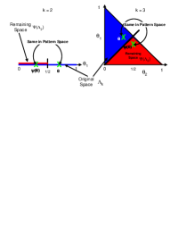
Figure 2: Transformation from i.i.d. space $\Lambda_{k}$ to pattern space $\Psi\left(\Lambda_{k}\right)$ for $k=2$ and $k=3$

In order to lower bound the size $M$ of the grid $\Psi\left(\mbox{\boldmath$\Omega$}\right)$, we need to take out from $\Omega$ any point $\mbox{\boldmath$\theta$}\in\mbox{\boldmath$\Omega$}$ that is a non-identity permutation of $\mbox{\boldmath$\psi$}\left(\mbox{\boldmath$\theta$}\right)$. For each point in $\Psi\left(\mbox{\boldmath$\Omega$}\right)$, there are at most $k!$ such permutations (although there may be less). Therefore, we can lower bound the logarithm of $M$, using Stirling’s approximation and (39), by

$$\log M \geq \log M_{\mbox{i.i.d.}}-\log\left(k!\right)$$ (40)

$$\geq \frac{k-1}{2}\log\frac{n^{1-\varepsilon^{\prime}}}{k^{3}}+\frac{k-1}{2}\log\frac{\pi e^{3}}{2}-2\log k-O(1).$$

From (40), we note that there exists a constant $c$ such that if $k>cn^{(1-\varepsilon^{\prime})/3}$ the bound above becomes negative. The reason is that we eliminated many points from the grid more than once. For example, the grid point $\mbox{\boldmath$\theta$}=\left[\tau_{1},\tau_{1},\cdots,\tau_{1}\right]$ only appears once in the grid $\Omega$ but was reduced by a factor of $k!$ times to obtain the bound in (40). This problem is negligible for small $k$’s, because such grid points make a negligible fraction of $\Omega$. However, for large $k$’s, almost all or all (for very large $k$’s) grid points contain many components that are identical.

To achieve a more useful bound on the logarithm of the number of grid points for large alphabets, we can find the value of $k$ for which the maximal lower bound is obtained from (40). Denote it by $k_{m}$. Then, for $k>k_{m}$ (including $k>n$), we can fix the first $k-k_{m}$ components of $\theta$ at a value of $o\left[1/(n^{1+\varepsilon}(k-k_{m}))\right]$ for all points in $\mbox{\boldmath$\theta$}\in\Psi\left(\mbox{\boldmath$\Omega$}\right)$, where the $i$th component, $i\leq k-k_{m}$, of all $\mbox{\boldmath$\theta$}\in\Psi\left(\mbox{\boldmath$\Omega$}\right)$ takes the same value, and any of these letters will appear in $x^{n}$ with probability going to $0$. The other $k_{m}$ components will take the values from a pattern grid for alphabet of size $k_{m}$. Note that now we can justify the assumption that $k_{m}\leq n^{1-2\varepsilon}$, assumed earlier for computing the number of grid points. In fact, $k_{m}$ is much smaller as indicated earlier. However, by fixing all other components of $\theta$ as described above, the bound for $k_{m}$ applies even for alphabets with $k>n^{1-2\varepsilon}$. If we now show that all points are distinguishable in the grid for $k=k_{m}$, they will also be distinguishable in the grid defined above for larger $k$. Therefore, the bound for $k_{m}$ will hold for every larger $k$ as well.

The bound in (40) attains a maximum value for $k_{m}=\left(\pi/2\right)^{1/3}\cdot n^{(1-\varepsilon^{\prime})/3}\approx 1.16n^{(1-\varepsilon^{\prime})/3}$. Substituting $k_{m}$ in (40), normalizing by $n$, and replacing $\varepsilon^{\prime}$ by $\varepsilon$, we obtain the second region of the bound in (30). The first region of the bound is obtained by normalizing the bound in (40) by $n$ and substituting $\varepsilon^{\prime}$ by $\varepsilon$. To conclude the proof of Theorem 1, we only need to prove distinguishability in the non-uniform pattern grid. By the weak version of the redundancy-capacity theorem, if distinguishability is proved, then the bounds we have obtained lower bound the minimax redundancy.

We will now show that distinguishability in the grid $\Psi\left(\mbox{\boldmath$\Omega$}\right)$ is a direct result of the distinguishability in the grid $\Omega$. Let the sequence $X^{n}$ be generated by the point $\mbox{\boldmath$\theta$}=\mbox{\boldmath$\psi$}\left(\mbox{\boldmath$\theta$}\right)\in\Psi\left(\mbox{\boldmath$\Omega$}\right)$. Let $\Psi\left(X^{n}\right)$ be the pattern of $X^{n}$. Consider the estimator $\mbox{\boldmath$\psi$}\left(\hat{\mbox{\boldmath$\theta$}}\right)$ of $\theta$ obtained as a function of $\Psi\left(X^{n}\right)$, and let $\hat{\mbox{\boldmath$\theta$}}^{\psi}_{\Omega}$ be the nearest point to $\mbox{\boldmath$\psi$}\left(\hat{\mbox{\boldmath$\theta$}}\right)$ on the grid $\Psi\left(\mbox{\boldmath$\Omega$}\right)$. We will show that there is an estimator $\mbox{\boldmath$\psi$}\left(\hat{\mbox{\boldmath$\theta$}}\right)$ for which $P_{\theta}\left(\hat{\mbox{\boldmath$\theta$}}^{\psi}_{\Omega}\neq\mbox{\boldmath$\theta$}\right)\rightarrow 0$ as $n\rightarrow\infty$. By definition of $\Psi\left(\mbox{\boldmath$\Omega$}\right)$, the components $\theta_{i};1\leq i\leq k,$ of $\theta$ are in non-decreasing order. Let $\hat{\mbox{\boldmath$\theta$}}$ be the ML estimator of $\theta$ from $X^{n}$, and $\hat{\mbox{\boldmath$\theta$}}_{\Omega}$ the closest point in $\Omega$ to $\hat{\mbox{\boldmath$\theta$}}$ that is used to estimate $\theta$ in the standard i.i.d. case. Let $\mbox{\boldmath$\psi$}\left(\hat{\mbox{\boldmath$\theta$}}\right)$ be the ordered permutation of $\hat{\mbox{\boldmath$\theta$}}$, that can be obtained directly from the pattern $\Psi\left(X^{n}\right)$. For every $\theta_{i}$, $i=1,\ldots,k$, let $\tau_{b_{i}}$ be the nearest point in $\tau$ to $\theta_{i}$ that is smaller than or equal to $\theta_{i}$. (Note that for $i<k$, $\tau_{b_{i}}=\theta_{i}$, and only for $\theta_{k}$ it may be smaller than $\theta_{k}$.) Define the event $A_{i}$ as

$$A_{i}~{}:~{}\left|\hat{\theta}_{i}-\theta_{i}\right|\geq\frac{\Delta\left(\tau_{b_{i}}\right)}{2},$$ (41)

i.e., the event in which the ML estimate of component $\theta_{i}$ is outside an interval of length $\Delta\left(\tau_{b_{i}}\right)$ centered at $\theta_{i}$. (If an error occurs in estimating $\theta_{i}$ by $\hat{\theta}_{\Omega i}$, this must be true because $\Delta\left(\tau_{b_{i}}\right)/2$ is at most half the distance between $\theta_{i}$ and its nearest neighbors.) Let event $\Psi\left(A_{i}\right)$ be defined as

$$\Psi\left(A_{i}\right)~{}:~{}\left|\mbox{\boldmath$\psi$}_{i}\left(\hat{\mbox{\boldmath$\theta$}}\right)-\theta_{i}\right|\geq\frac{\Delta\left(\tau_{b_{i}}\right)}{2},$$ (42)

where $\mbox{\boldmath$\psi$}_{i}\left(\hat{\mbox{\boldmath$\theta$}}\right)$ denotes the $i$th ordered component of the ML estimate of $\theta$, where the components are ordered in non-decreasing order. Define event $A\stackrel{{\scriptstyle\triangle}}{{=}}\bigcup_{i}A_{i}$ as the union of all events $A_{i}$ and event $\Psi\left(A\right)\stackrel{{\scriptstyle\triangle}}{{=}}\bigcup_{i}\Psi\left(A_{i}\right)$ as the union of all events $\Psi\left(A_{i}\right)$. The probability that event $A$ occurs when $X^{n}$ is generated by $\theta$ will be denoted by $P_{\theta}\left(A\right)$. In a similar manner, $P_{\theta}\left[\Psi\left(A\right)\right]$ will denote the probability that $\Psi\left(A\right)$ occurs given $X^{n}$ is generated by $\theta$. By definition of $\Psi\left(A\right)$ and (42), event $\Psi\left(A\right)$ implies that the ordered version $\mbox{\boldmath$\psi$}\left(\hat{\mbox{\boldmath$\theta$}}\right)$ of the ML estimator $\hat{\mbox{\boldmath$\theta$}}$ is outside the portion in $\Psi\left(\Lambda_{k}\right)$ of the box with edges $\Delta\left(\tau_{b_{i}}\right)$, for every $i$, centered at $\theta$. The following lemma, which is proved in Appendix B, bounds $P_{\theta}\left(A\right)$:

Lemma 5.2

$$P_{\theta}\left(A\right)\leq 2^{(\log k)+(\log n)-cn^{\varepsilon/2}}\rightarrow 0,$$ (43)

where $c$ is a constant.

Note that $P_{\theta}\left(A\right)\geq P_{\theta}\left(\hat{\mbox{\boldmath$\theta$}}_{\Omega}\neq\mbox{\boldmath$\theta$}\right)$, but we require a bound on the larger probability in order to apply it to the pattern space. In the standard i.i.d. case, there is thus a vanishing probability even to estimating $\theta$ outside the defined box. The following lemma relates between the probability of event $\Psi\left(A\right)$ and that of event $A$.

Lemma 5.3

$$P_{\theta}\left[\Psi\left(A\right)\right]\leq P_{\theta}\left(A\right).$$ (44)

Proof: We show that $\bar{A}\rightarrow\left(\overline{\Psi\left(A\right)}\cap B\right)$, where $\bar{A}$ is the complement to $A$, and event $B$ is defined below. Therefore, $\left[\Psi\left(A\right)\cup\bar{B}\right]=\left\{\left[\Psi\left(A\right)\cap B\right]\cup\bar{B}\right\}\rightarrow A$, and thus also $\Psi\left(A\right)\rightarrow A$ and $P_{\theta}\left\{\Psi\left(A\right)\right\}\leq P_{\theta}\left(A\right)$. The proof consists of the following steps: First, let $\mbox{\boldmath$\varphi$}\subseteq\left(\theta_{1},\theta_{2},\ldots,\theta_{k-1},\tau_{b_{k}}\right)$ be a subset of $\theta$ with $\theta_{k}$ replaced by the nearest smaller grid point. Let $\varphi$ consist only of distinct (unequal) elements. Let the components of $\varphi$ be ordered in increasing order. We show that $\bar{A}$ implies that $\hat{\mbox{\boldmath$\varphi$}}$ is also in increasing order for any choice of $\varphi$ as described above. The latter event is denoted by $B$. Hence, the respective ordered components of $\mbox{\boldmath$\psi$}\left(\hat{\mbox{\boldmath$\varphi$}}\right)$ will not be permuted from those of $\hat{\mbox{\boldmath$\varphi$}}$. This means that if $\mbox{\boldmath$\psi$}\left(\hat{\mbox{\boldmath$\varphi$}}\right)\neq\hat{\mbox{\boldmath$\varphi$}}$ (i.e., $\mbox{\boldmath$\psi$}\left(\hat{\mbox{\boldmath$\varphi$}}\right)$ is a non-identity permutation of $\hat{\mbox{\boldmath$\varphi$}}$ and event $\bar{B}$ occurs), $A$ must occur. Then, we show that for equal components of $\theta$, although the components of $\hat{\mbox{\boldmath$\theta$}}$ may not be ordered, if $\bar{A}$ is satisfied, then each of the ordered components of $\mbox{\boldmath$\psi$}\left(\hat{\mbox{\boldmath$\theta$}}\right)$ must satisfy $\overline{\Psi\left(A_{i}\right)}$. Together with the first step, this means that given $\bar{A}$, at least $k-2$ components of $\mbox{\boldmath$\psi$}\left(\hat{\mbox{\boldmath$\theta$}}\right)$ must satisfy event $\overline{\Psi\left(A_{i}\right)}$. The only remaining components of $\mbox{\boldmath$\psi$}\left(\hat{\mbox{\boldmath$\theta$}}\right)$ consist of at most $\mbox{\boldmath$\psi$}_{k}\left(\hat{\mbox{\boldmath$\theta$}}\right)$ and one more component $\mbox{\boldmath$\psi$}_{l}\left(\hat{\mbox{\boldmath$\theta$}}\right)$ which takes the value of $\hat{\theta}_{k}$ if $\hat{\theta}_{k}$ is not the maximal ML component of $\hat{\mbox{\boldmath$\theta$}}$. (Otherwise, the proof is complete.) For these two components, we show that $\left\{\left[\Psi\left(A_{l}\right)\cup\Psi\left(A_{k}\right)\right]\cap B\right\}\rightarrow A$, concluding the proof.

First, assume that $\bar{A}$ occurs. Then, for all $i;1\leq i\leq k$,

$$\left|\hat{\theta}_{i}-\theta_{i}\right|<\frac{\Delta\left(\tau_{b_{i}}\right)}{2}~{}\Rightarrow~{}-\frac{\Delta\left(\tau_{b_{i}}\right)}{2}<\hat{\theta}_{i}-\theta_{i}<\frac{\Delta\left(\tau_{b_{i}}\right)}{2}.$$ (45)

Let $\tau_{b_{j}}>\tau_{b_{i}}$. Note that by definition of $\theta$ as an ordered vector and of $\tau_{b}$, $\tau_{b_{j}}>\tau_{b_{i}}$ implies that $\theta_{j}>\theta_{i}$ (and also that $j>i$). (The other direction is true for $j<k$.) Given $\bar{A}$, we thus have,

$$\hat{\theta}_{j}-\hat{\theta}_{i}=\left(\hat{\theta}_{j}-\theta_{j}\right)+\left(\theta_{j}-\theta_{i}\right)+\left(\theta_{i}-\hat{\theta}_{i}\right)>-\frac{\Delta\left(\tau_{b_{j}}\right)}{2}+\Delta\left(\tau_{b_{j}}\right)-\frac{\Delta\left(\tau_{b_{i}}\right)}{2}>0,$$ (46)

where the first inequality is obtained by applying the left hand side of inequality (45) to the first two and the last two terms, respectively, and by applying the left hand side of (33) to the two middle terms. The last inequality is from the monotonicity of $\Delta\left(\tau_{b}\right)$ in $b$. Hence, if $\tau_{b_{j}}>\tau_{b_{i}}$, then $\bar{A}$ implies that we must also have $\hat{\theta}_{j}>\hat{\theta}_{i}$ (and event $B$ must occur). This means that if the ML estimates of two letters separated by at least one grid spacing unit are within the boxes defined in (45), then these ML estimates are still ordered in the same order as the original letters. Hence, the only case where ML estimates of two different letters may not be in the original order of the letters is when $\tau_{b_{j}}=\tau_{b_{i}}$ for $j>i$. For $j<k$, this implies also that $\theta_{j}=\theta_{i}$, and thus if $\mbox{\boldmath$\psi$}_{i}\left(\hat{\mbox{\boldmath$\theta$}}\right)=\hat{\theta}_{j}$ but also (45) holds for $\theta_{j}$, then,

$$\left|\mbox{\boldmath$\psi$}_{i}\left(\hat{\mbox{\boldmath$\theta$}}\right)-\theta_{i}\right|=\left|\hat{\theta}_{j}-\theta_{i}\right|=\left|\hat{\theta}_{j}-\theta_{j}\right|<\frac{\Delta\left(\tau_{b_{j}}\right)}{2}=\frac{\Delta\left(\tau_{b_{i}}\right)}{2}.$$ (47)

Therefore, for all $i\leq k$, except for at most $i=k$ and one value $i=l<k$, for which $\tau_{b_{l}}=\tau_{b_{k}}$, if $\bar{A}$ occurs, also $\overline{\Psi\left(A_{i}\right)}$ occurs. This is because except for permutations with $\hat{\theta}_{k}$, the only permutations violating the order of $\theta$ in the resulting $\hat{\mbox{\boldmath$\theta$}}$ can occur between letters with equal probabilities in $\theta$. From the last inequality, such permutations still result in occurrence of $\overline{\Psi\left(A_{i}\right)}$.

The only case in which $\theta_{j}>\theta_{i}$ does not necessarily imply $\hat{\theta}_{j}>\hat{\theta}_{i}$ is when $j=k$ and $\tau_{b_{i}}=\tau_{b_{k}}$. Let us now consider this case when $\hat{\theta}_{k}$ is not the maximal component of $\hat{\mbox{\boldmath$\theta$}}$. (If $\hat{\theta}_{k}$ is the maximal component of $\hat{\mbox{\boldmath$\theta$}}$, the order of the estimates in $\hat{\mbox{\boldmath$\theta$}}$ is not violated beyond permutations of equal components in $\theta$, and we are back in the previous cases, for which the lemma has already been proved.) Let $\hat{\theta}_{i}$ be the maximum component of $\hat{\mbox{\boldmath$\theta$}}$. Then, $\mbox{\boldmath$\psi$}_{k}\left(\hat{\mbox{\boldmath$\theta$}}\right)=\hat{\theta}_{i}$. Also, there exists $l$, for which $\tau_{b_{l}}=\tau_{b_{k}}$, such that $\mbox{\boldmath$\psi$}_{l}\left(\hat{\mbox{\boldmath$\theta$}}\right)=\hat{\theta}_{k}$. We show that if either $\Psi\left(A_{l}\right)$ or $\Psi\left(A_{k}\right)$ occur together with $B$, then either $A_{i}$ or $A_{k}$ must occur as well.

First, let $\Psi\left(A_{k}\right)$ occur, i.e.,

$$\left|\hat{\theta}_{i}-\theta_{k}\right|\geq\frac{\Delta\left(\tau_{b_{k}}\right)}{2}.$$ (48)

If $\hat{\theta}_{i}>\theta_{k}$,

$$\hat{\theta}_{i}-\theta_{i}=\left(\hat{\theta}_{i}-\theta_{k}\right)+\left(\theta_{k}-\theta_{i}\right)\geq\frac{\Delta\left(\tau_{b_{k}}\right)}{2},$$ (49)

where the inequality is by definition of this case and by the ordering of $\theta$. The last inequality means that $A_{i}$ occurs. If $\hat{\theta}_{i}<\theta_{k}$,

$$\theta_{k}-\hat{\theta}_{k}=\left(\theta_{k}-\hat{\theta}_{i}\right)+\left(\hat{\theta}_{i}-\hat{\theta}_{k}\right)\geq\frac{\Delta\left(\tau_{b_{k}}\right)}{2},$$ (50)

where the inequality is, again, by definition of the case, and by the assumption that $\hat{\theta}_{i}$ is the maximum component of the ML estimate of $\theta$. This inequality implies that $A_{k}$ occurs. Now, let $\Psi\left(A_{l}\right)$ occur for $l$ defined above. Then,

$$\left|\mbox{\boldmath$\psi$}_{l}\left(\hat{\mbox{\boldmath$\theta$}}\right)-\theta_{l}\right|=\left|\hat{\theta}_{k}-\theta_{l}\right|\geq\frac{\Delta\left(\tau_{b_{l}}\right)}{2}=\frac{\Delta\left(\tau_{b_{k}}\right)}{2}=\frac{\Delta\left(\tau_{b_{i}}\right)}{2},$$ (51)

where the equalities are since the occurrence of $B$ implies $\tau_{b_{l}}=\tau_{b_{k}}=\tau_{b_{i}}$. If $\hat{\theta}_{k}<\theta_{l}$,

$$\theta_{k}-\hat{\theta}_{k}=\left(\theta_{k}-\theta_{l}\right)+\left(\theta_{l}-\hat{\theta}_{k}\right)\geq\frac{\Delta\left(\tau_{b_{l}}\right)}{2}=\frac{\Delta\left(\tau_{b_{k}}\right)}{2},$$ (52)

where the inequality is obtained similarly to the previous cases. The last equality is from the occurrence of $B$. This implies that $A_{k}$ occurs. If $\hat{\theta}_{k}>\theta_{l}$, in a similar manner,

$$\hat{\theta}_{i}-\theta_{i}=\left(\hat{\theta}_{i}-\hat{\theta}_{k}\right)+\left(\hat{\theta}_{k}-\theta_{i}\right)=\left(\hat{\theta}_{i}-\hat{\theta}_{k}\right)+\left(\hat{\theta}_{k}-\theta_{l}\right)\geq\frac{\Delta\left(\tau_{b_{l}}\right)}{2}=\frac{\Delta\left(\tau_{b_{i}}\right)}{2},$$ (53)

where the second and last equalities are because of the occurrence of $B$. This implies $A_{i}$ occurs, and concludes the proof of Lemma 5.3. $\Box$

The proof of Lemma 5.3 considered three different cases relating between two components $\theta_{i}$ and $\theta_{j}$; $j>i$, of $\theta$. Figure 3 shows the projection of these three cases onto a two dimensional subspace that contains only components $i$ and $j$. The dots represent grid points. A rectangular box surrounding a dot contains all the ML estimator points that are in event $\bar{A}_{i}\cap\bar{A}_{j}$ if $(\theta_{i},\theta_{j})$ is on the dot. The first two cases are in part $(a)$ of the figure, and the last in part $(b)$. In the first case, the complete box is contained in $\Psi\left(\Lambda_{k}\right)$. This is the case in which $\theta_{j}>\theta_{i};j<k$. The occurrence of $\bar{A}$ implies event $B$, which means that the ML estimates in this case will remain in the original ordering, i.e., estimating the components of $\mbox{\boldmath$\psi$}\left(\hat{\mbox{\boldmath$\theta$}}\right)$ out of $\Psi\left(X^{n}\right)$ will give the same estimates as those obtained by estimating $\hat{\mbox{\boldmath$\theta$}}$ out of $X^{n}$. Note that $P_{\theta}\left\{\Psi\left(A_{i}\right)\cup\Psi\left(A_{j}\right)\right\}\leq P_{\theta}\left(A_{i}\cup A_{j}\right)$, where a possible decrease is because some un-typical sequences that have ML estimates $\hat{\mbox{\boldmath$\theta$}}\not\in\Psi\left(\Lambda_{k}\right)$ will be projected into the same box around $\theta$ by estimating out of $\Psi\left(X^{n}\right)$ and will (insignificantly) increase the probability of $\overline{\Psi\left(A_{i}\right)\cup\Psi\left(A_{j}\right)}$ from that of $\overline{A_{i}\cup A_{j}}$.

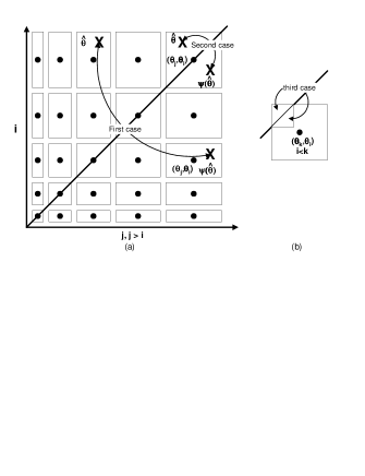
Figure 3: Decision regions in a two dimensional projection of the pattern grid $\Psi\left(\mbox{\boldmath$\Omega$}\right)$

In the second and third cases, the box around $\theta$ contains a region that is in $\Lambda_{k}$ but outside $\Psi\left(\Lambda_{k}\right)$, i.e., there exist sequences $x^{n}$ that can be generated by $\theta$ and result in an ML i.i.d. estimator $\hat{\mbox{\boldmath$\theta$}}$ of $\theta$ that is still within the box defined above, but is not properly ordered, and thus $\mbox{\boldmath$\psi$}\left(\hat{\mbox{\boldmath$\theta$}}\right)\neq\hat{\mbox{\boldmath$\theta$}}$. As shown in the proof of Lemma 5.3, this can only occur when $\theta_{i}=\theta_{j}$, as in the second case in Figure 3, or when $j=k$, and $\tau_{b_{i}}=\tau_{b_{k}}$, as shown in the third case of Figure 3. As shown in the proof of Lemma 5.3, both cases still result in $\bar{A}\rightarrow\overline{\Psi\left(A\right)}$ when estimation is done according to $\Psi\left(x^{n}\right)$. From Figure 3, we see that this is the case, because the re-ordering of $\hat{\mbox{\boldmath$\theta$}}$ to generate $\mbox{\boldmath$\psi$}\left(\hat{\mbox{\boldmath$\theta$}}\right)$ means projection of components of $\hat{\mbox{\boldmath$\theta$}}$ over the diagonal lines as shown for both cases in the figure.

To conclude the proof of Theorem 1, we need to consider the estimator $\hat{\mbox{\boldmath$\theta$}}^{\psi}_{\Omega}\in\Psi\left(\mbox{\boldmath$\Omega$}\right)$, which estimates $\mbox{\boldmath$\theta$}=\mbox{\boldmath$\psi$}\left(\mbox{\boldmath$\theta$}\right)$ by the point in $\Psi\left(\mbox{\boldmath$\Omega$}\right)$ nearest to $\mbox{\boldmath$\psi$}\left(\hat{\mbox{\boldmath$\theta$}}\right)$. Based on Lemmas 5.2 and 5.3, we show that the error probability for this estimator, which is solely based on the pattern $\Psi\left(X^{n}\right)$ of $X^{n}$, vanishes with $n$. An error occurs if $\hat{\mbox{\boldmath$\theta$}}^{\psi}_{\Omega}\neq\mbox{\boldmath$\theta$}$. If this happens, event $\Psi\left(A\right)$ must happen, because the distance between two adjacent grid points is not smaller than $2\Delta\left(\tau_{b_{i}}\right)/2=\Delta\left(\theta_{i}\right)$. (Note that now we only need to estimate the first $k-1$ components of $\theta$, since the last component $\theta_{k}$ is then determined by the others). Also, for the second region of the bound, no error is possible in the first $k-k_{m}$ small parameters because they need not be estimated since they are equal for all points on the grid $\Psi\left(\mbox{\boldmath$\Omega$}\right)$, and the probability that any of these letters occurs vanishes. Hence,

$$P_{\theta}\left(\hat{\mbox{\boldmath$\theta$}}^{\psi}_{\Omega}\neq\mbox{\boldmath$\theta$}\right)\leq P_{\theta}\left[\Psi\left(A\right)\right]\leq P_{\theta}\left(A\right)\rightarrow 0.$$ (54)

This concludes the proof of Theorem 1. $\Box$

6 A Lower Bound for Most Sources

The analysis in Section 5 cannot be used to lower bound the average pattern redundancy for most sources. This is because of the non-uniform grid. The strong version of the redundancy-capacity theorem requires the sources in each set of $M$ sources to be uniformly distributed for the result in (25) to hold. However, randomly choosing a non-uniform grid, generating a uniform distribution of the sources in the grid, results in an overall non-uniform distribution of the sources in $\Psi\left(\Lambda_{k}\right)$, because sources in the dense areas are more likely to be chosen. The redundancy-capacity theorem can still be used, but the bound that is obtained will be a bound on the class, assuming the sources are distributed with a non-uniform prior in the class $\Psi\left(\Lambda_{k}\right)$. Such a bound is not a bound for most sources in the class in Rissanen’s sense.

To derive a lower bound on the redundancy for most sources in the class $\Psi\left(\Lambda_{k}\right)$, a different approach from that in Section 5 must, therefore, be used. Instead of a non-uniform grid, we show that sources in the centers of disjoint spheres with radius $r=n^{-0.5(1-\varepsilon)}$ in the $k-1$ dimensional pattern space are distinguishable, and count the number of spheres that can be packed in the space $\Psi\left(\Lambda_{k}\right)$ (see [2] for information about the sphere packing problem). This sphere lattice can be shifted to cover the whole class for different choices of $M$ points. Hence, the conditions of the strong version of the redundancy-capacity theorem are then satisfied, and the normalized logarithm of the bound on the number of spheres becomes the lower bound on the redundancy for most sources. (This approach resembles Rissanen’s pioneering work [24] for sources with a finite number of parameters. However, here the asymptotics change due to the consideration of patterns and large alphabets.)

Since we no longer take advantage of the fact that sources that vary only in small parameters are still distinguishable, the size of the grid that is constructed reduces w.r.t. that of the minimax bound. This leads to a smaller lower bound on the redundancy for most sources, hinting that it may be possible to compress most sources in the class better than the worst sources. This is reasonable because many sources, with large $k$ in particular, may generate very compressible pattern sequences, that may decrease the overall average redundancy. On the other hand, however, this redundancy reduction may also be due to looseness in the bounding techniques. The orders of the bounds obtained remain the same as those of the minimax bound, but for large alphabets, the coefficients become smaller. For small alphabets, the decrease in the bound is reflected in a smaller second order term. We proceed with Theorem 2, that lower bounds the redundancy of patterns generated by most sources in the class $\Lambda_{k}$ and conclude this section with its proof.

Theorem 2

Fix an arbitrarily small $\varepsilon>0$, and let $n\rightarrow\infty$. Then, the $n$th-order average universal coding redundancy for coding patterns induced by i.i.d. sources with alphabet size $k$ is lower bounded by

$$R_{n}\left[L,\mbox{\boldmath$\psi$}\left(\mbox{\boldmath$\theta$}\right)\right]\geq\left\{\begin{array}[]{ll}\frac{k-1}{2n}\log\frac{n^{1-\varepsilon}}{k^{3}}-\frac{k-1}{2n}\log\frac{8\pi}{e^{3}}-O\left(\frac{\log k}{n}\right),&\mbox{for }k\leq\frac{1}{2}\cdot\left(\frac{n^{1-\varepsilon}}{\pi}\right)^{1/3}\\ \frac{1.5\log e}{2\pi^{1/3}}\cdot n^{-(2+\varepsilon)/3}-O\left(\frac{\log n}{n}\right),&\mbox{for }k>\frac{1}{2}\cdot\left(\frac{n^{1-\varepsilon}}{\pi}\right)^{1/3}\end{array}\right.$$ (55)

for every code $L(\cdot)$ and almost every i.i.d. source $\mbox{\boldmath$\theta$}\in\Lambda_{k}$, except for a set of sources $A_{\varepsilon}\left(n\right)$ whose volume goes to $0$ as $n\rightarrow\infty$.

Theorem 2 shows similar behavior of the redundancy for most sources to that shown by Theorem 1 for the minimax redundancy. For small $k$, each probability parameter, again, costs $0.5\log(n/k^{3})$ extra code bits. For large $k$’s (including $k>n$), we obtain a redundancy bound of $O\left(n^{-2/3}\right)$, identical for all large values of $k$. The lower bound of Theorem 2 naturally is the strongest sense bound and applies also to the minimax average and individual redundancies. It is therefore smaller than the other two sets of bounds. While the first order term in the first region of (55) is equal to that of (30), the second order term here is negative and decreases the redundancy for most sources linearly with $k$, whereas the second order term of the first region in (30) is positive and increases the minimax redundancy linearly with $k$. In the second region of the bound in (55), the coefficient of the redundancy which approximately equals $0.74$ decreases w.r.t. that of the minimax redundancy in (30), which approximately equals $2.52$.

The proof of Theorem 2 lower bounds the volume of the space $\Psi\left(\Lambda_{k}\right)$, and then uses sphere packing density results [2] to lower bound the number of spheres that can be packed in this volume. Then, it is shown that sources at centers of disjoint spheres with radius $r=n^{-0.5(1-\varepsilon)}$ are distinguishable also in the pattern space, i.e., by observing $\Psi\left(X^{n}\right)$. There are two methods that bound the volume of the space $\Psi\left(\Lambda_{k}\right)$. The first takes the volume of $\Lambda_{k}$, which by condition (35) must be $1/(k-1)!$, and divides it by $k!$ to extract all permutations of the same sources, resulting in a volume of $1/[(k-1)!k!]$. The other method directly computes the volume of $\Psi\left(\Lambda_{k}\right)$ from the conditions defining an ordered vector $\mbox{\boldmath$\psi$}\left(\mbox{\boldmath$\theta$}\right)$. Both methods obtain the same bound on the volume of $\Psi\left(\Lambda_{k}\right)$. We will, therefore, demonstrate only the second one. Since the second method is tight, it hints to the fact that, unlike the reduction of the grid $\Omega$ in Section 5 by a factor of $k!$ to form the grid $\Psi\left(\mbox{\boldmath$\Omega$}\right)$, the reduction of the volume of $\Lambda_{k}$ by a factor of $k!$ to bound the volume of $\Psi\left(\Lambda_{k}\right)$ is tight. This is because of the difference in considering a grid and a continuous space. In the continuous space $\Lambda_{k}$, sources with several exactly identical components make a negligible portion of the space (as the probability of any single point is zero), whereas such sources are not negligible when we construct a grid as in Section 5.

Although the bounding of the volume of $\Psi\left(\Lambda_{k}\right)$ is tight, we still encounter a similar phenomenon to that in Section 5, where there exists a constant $c$, such that for every $k>cn^{(1-\varepsilon)/3}$, the bound becomes negative. This is due to another step in the bounding. In this analysis, we bound the number of spheres packed in $\Psi\left(\Lambda_{k}\right)$ dividing the volume of $\Psi\left(\Lambda_{k}\right)$ by a volume of a single sphere and factoring a packing density factor. However, as $k$ increases, most spheres contained in $\Psi\left(\Lambda_{k}\right)$ have only portions in the space, whereas big portions of those spheres are outside the space. Therefore, division by the complete volume of a sphere results in loose bounding of the number of sources that are still distinguishable in the space. We solve this problem in a manner that resembles the solution in Section 5. Let $k_{m}$ be the value of $k$ for which the bound is maximal. Then, for $k>k_{m}$, instead of considering the whole space $\Psi\left(\Lambda_{k}\right)$ and bounding the number of spheres in it, we bound the number of spheres in a slice of this space, in which there are only $k_{m}$ sufficiently large probability parameters, and all the other $k-k_{m}$ probability parameters sum to an insignificantly small total probability. This idea is best pictured if one considers packing spheres in a triangular based pyramid. The number of circles that can be packed on its basis is larger than the number of circles that can be packed in any horizontal two dimension cut above the basis. If the spheres are very large, we may not be able to pack any complete two dimensional cuts of these spheres above the basis. Since we are not interested in complete spheres in all dimensions, it is sufficient to consider the number of dimensions that will give the maximum number of sphere portions that are packed in the space. This number is a lower bound on the total number of sphere portions that can be packed in the space. Using only $k_{m}$ dimensions in the sphere packing analysis, we obtain the second region of the bound. Note that when we shift the sphere lattice to obtain a covering of the whole space, some center points that represent sources in the set will no longer be in the space, reducing $M$. However, the lower bound on $M$ obtained from the $k_{m}$ dimensional cut will not be affected, when at the same time the shifting allows the space covering condition of the strong version of the redundancy-capacity theorem to be satisfied.

As in Section 5, we also need to show that distinguishability in the i.i.d. space carries over to the pattern space. This is, in fact, easier than in the minimax case. All we need to show is that a point $\hat{\mbox{\boldmath$\theta$}}$ in $\Lambda_{k}$ outside $\Psi\left(\Lambda_{k}\right)$ but still in a sphere that is centered inside $\Psi\left(\Lambda_{k}\right)$ projects onto a point $\mbox{\boldmath$\psi$}\left(\hat{\mbox{\boldmath$\theta$}}\right)$ that is still in the same sphere. The point $\mbox{\boldmath$\psi$}\left(\hat{\mbox{\boldmath$\theta$}}\right)$ is the one that will be obtained directly from $\Psi\left(X^{n}\right)$. Therefore, if the ML i.i.d. estimator $\hat{\mbox{\boldmath$\theta$}}$ of $\theta$ based on $X^{n}$ is outside $\Psi\left(\Lambda_{k}\right)$ but still distinguishable in the i.i.d. space, its projection $\mbox{\boldmath$\psi$}\left(\hat{\mbox{\boldmath$\theta$}}\right)$ into $\Psi\left(\Lambda_{k}\right)$, obtained from $\Psi\left(X^{n}\right)$, is still in the same sphere. This is shown by geometric considerations demonstrated as a series of exchanges that rearrange the components of $\hat{\mbox{\boldmath$\theta$}}$ into $\mbox{\boldmath$\psi$}\left(\hat{\mbox{\boldmath$\theta$}}\right)$ by exchanging a pair in each step. We conclude this section with the proof of Theorem 2.

Proof of Theorem 2: We begin with bounding the volume of the $k-1$ dimensional space $\Psi\left(\Lambda_{k}\right)$. Only ordered vectors $\theta$ for which $\theta_{1}\leq\theta_{2}\leq\cdots\leq\theta_{k-1}$ are contained in $\Psi\left(\Lambda_{k}\right)$. This can be used to set constraints on a $k-1$ dimensional integral that bounds the volume of $\Psi\left(\Lambda_{k}\right)$. By condition (35),

$$1\geq\sum_{i=1}^{k-1}\theta_{i}\geq\left(k-1\right)\theta_{1}~{}\Rightarrow~{}\theta_{1}\leq\frac{1}{k-1}.$$ (56)

Similarly (and more generally),

$$1-\sum_{j=1}^{i-1}\theta_{j}\geq\sum_{l=i}^{k-1}\theta_{l}\geq(k-i)\theta_{i}~{}\Rightarrow~{}\theta_{i}\leq\frac{1-\sum_{j=1}^{i-1}\theta_{j}}{(k-i)}.$$ (57)

Now, (57) gives upper limits on every component of $\theta$. The ordering condition of $\theta$ that is necessary for $\theta$ to be in $\Psi\left(\Lambda_{k}\right)$ gives lower limits on each component of $\theta$. Ordering is maintained by the above conditions except for the $k$th component $\theta_{k}$. Therefore, the volume obtained by a $k-1$ dimensional integral over $1$ within all these limits needs to be reduced by a factor of $k$ to only take the $k$ dimensional permutations for which $\theta_{k}$ is not smaller than all other components of $\theta$. Including all the constraints, $V\left[\Psi\left(\Lambda_{k}\right)\right]$ is computed in the following equations:

$$V\left[\Psi\left(\Lambda_{k}\right)\right] = \frac{1}{k}\cdot\int_{0}^{\frac{1}{k-1}}d\theta_{1}\int_{\theta_{1}}^{\frac{1}{k-2}\left(1-\theta_{1}\right)}d\theta_{2}\int_{\theta_{2}}^{\frac{1}{k-3}\left(1-\theta_{1}-\theta_{2}\right)}d\theta_{3}\cdots\int_{\theta_{k-2}}^{\frac{1}{1}\left(1-\theta_{1}-\theta_{2}-\cdots-\theta_{k-2}\right)}d\theta_{k-1}$$ (58)

$$= \cdots~{}~{}=\frac{1}{k}\cdot\int_{0}^{\frac{1}{k-1}}d\theta_{1}\left\{\frac{1}{\left[\left(k-2\right)!\right]^{2}}\left[1-\left(k-1\right)\theta_{1}\right]^{k-2}\right\}$$

$$= \frac{1}{k}\cdot\left[-\frac{1}{\left[\left(k-1\right)!\right]^{2}}\left[1-\left(k-1\right)\theta_{1}\right]^{k-1}\right]_{0}^{\frac{1}{k-1}}~{}=~{}\frac{k}{\left[k!\right]^{2}}~{}=~{}\frac{1}{\left(k-1\right)!\cdot k!}$$

Now, consider packing of $k-1$ dimensional spheres with radius $r=n^{-0.5\left(1-\varepsilon\right)}$ in $\Psi\left(\Lambda_{k}\right)$ so that no spheres share the same point in the space. The ratio between the volume $V\left[\Psi\left(\Lambda_{k}\right)\right]$ of $\Psi\left(\Lambda_{k}\right)$ and the volume of one sphere $V_{k-1}(r)$ is

$$\rho\stackrel{{\scriptstyle\triangle}}{{=}}\frac{V\left[\Psi\left(\Lambda_{k}\right)\right]}{V_{k-1}(r)}=\frac{1}{(k-1)!\cdot k!\cdot V_{k-1}(r)}=\left\{\begin{array}[]{ll}\frac{\left[\left(k-1\right)/2\right]!\cdot n^{\frac{1}{2}\left(1-\varepsilon\right)\left(k-1\right)}}{\pi^{(k-1)/2}\cdot\left(k-1\right)!\cdot k!};&k~{}\mbox{odd}\\ \frac{n^{\frac{1}{2}\left(1-\varepsilon\right)\left(k-1\right)}}{\left[\left(k-2\right)/2\right]!\cdot 2^{k-1}\cdot\pi^{(k-2)/2}\cdot k!};&k~{}\mbox{even},\end{array}\right.$$ (59)

where we substituted the volume of $\Psi\left(\Lambda_{k}\right)$ from (58). However, the number of spheres that can be packed in $\Psi\left(\Lambda_{k}\right)$ is bounded by

$$M\geq\Delta\rho\geq\frac{1}{(k-1)!\cdot k!\cdot V_{k-1}\left(r\right)\cdot 2^{k-1}},$$ (60)

where the factor $\Delta=2^{-(k-1)}$ is a lower bound on the sphere packing density, i.e., the fraction of the space that is actually occupied by spheres (see [2]). Now, let us choose a grid that contains the sources $\theta$ at the centers of all the $M$ spheres packed in $\Psi\left(\Lambda_{k}\right)$. We can lower bound the number of sources in one such grid by using (59)-(60). Taking the logarithm of the bound in (60) and using Stirling’s formula to bound factorials, we obtain the bound

$$\log M\geq\left(1-\varepsilon\right)\frac{k-1}{2}\log n-\frac{k-1}{2}\log k^{3}-\frac{k-1}{2}\log\frac{8\pi}{e^{3}}-\frac{3}{2}\log k+\frac{1}{2}\log\frac{e^{3}}{4\pi}-O\left(\frac{1}{k}\right).$$ (61)

As long as the lower bound on $M$ is large, we can (cyclicly) shift the whole grid to allow different choices of grids in $\Psi\left(\Lambda_{k}\right)$ to cover the whole space, and satisfy the conditions of the strong version of the redundancy-capacity theorem. All random shifts of the original grid will form a covering of $\Psi\left(\Lambda_{k}\right)$, and can be designed so that uniform distribution is preserved for choosing a point $\mbox{\boldmath$\theta$}\in\Psi\left(\Lambda_{k}\right)$ over the whole class and also within every set of $M$ points that is chosen. Hence, in this case we can use the normalized logarithm of the number $M$ of points on this random grid as a lower bound on the redundancy for most sources if all sources within any shift of the grid are distinguishable by the observed random sequence. This yields the first region of the bound in (55). However, observing (61), as in the minimax case, the bound becomes negative and useless for large $k$’s. As in Section 5, we solve this problem by fixing the bound at its maximum value as a function of $k$. Assume this value is attained at $k=k_{m}$. Then, for every $k>k_{m}$, we will obtain the same bound, resulting in the second region in (55). By straightforward differentiation it can be shown that the bound in (61) attains its maximum value for $k_{m}=0.5\left(n^{1-\varepsilon}/\pi\right)^{1/3}$. Substituting this value of $k_{m}$ in (61), normalizing by $n$, we obtain the bound of the second region of (55).

When $k_{m}$ is used to obtain the bound for a larger $k$, we still shift the complete grid to create a covering of the space $\Psi\left(\Lambda_{k}\right)$ in which each source is contained in one grid. Unlike the minimax case, here we cannot simply discard points in the grid with $k>k_{m}$ nonzero parameters. These must be included in the grid, and distinguishability between them and other points must be proven. However, we can lower bound the number of sources in the grid by the number of spheres in $k_{m}$ dimensional cut of $\Psi\left(\Lambda_{k}\right)$ for which all the other (first) $k-k_{m}$ parameters are very small, and insignificant. This analysis is valid also if $k>n$, and thus the bound in the second region is general, and applies also to such large alphabets.

Finally, to satisfy the covering of the whole space, we need to show that every source in $\Lambda_{k}$ is included in a grid. Demonstrating that only for the ordered permutation is not sufficient. This can be done by taking different grids for each permutation vector, i.e., each ordered source $\mbox{\boldmath$\psi$}\left(\mbox{\boldmath$\theta$}\right)$ will appear in $k!$ different grids through its permutations. (Since the probability of a single point is zero in a continuous space, sources for which identical components exist do not pose a problem.)

To conclude the proof of Theorem 2, we need to show distinguishability of the grids defined above in the pattern space. We show that this is a direct result of distinguishability of the respective grids in the i.i.d. space. First, we state a lemma showing distinguishability in the i.i.d. space, i.e., by observing $X^{n}$, and then we prove another lemma that implies that distinguishability in the i.i.d. space causes distinguishability in the pattern space on the reduced pattern grid, obtained by observing only $\Psi\left(X^{n}\right)$.

Lemma 6.1

Consider one choice of a random grid in the i.i.d. space $\Lambda_{k}$ as defined above. Let $\mbox{\boldmath$\theta$}\in\Lambda_{k}$ be a point on this grid, and let the random sequence $X^{n}$ be generated by the conditional probability $P_{\theta}(X^{n})$ (given $\theta$). Then, the probability that the ML estimator of $\theta$ from the observed $X^{n}$ is outside the sphere of radius $1/\sqrt{n}^{1-\varepsilon}$ centered in $\theta$ vanishes with $n$,

$$\lim_{n\rightarrow\infty}P_{\theta}\left\{\left\|\hat{\mbox{\boldmath$\theta$}}-\mbox{\boldmath$\theta$}\right\|>\frac{1}{\sqrt{n}^{1-\varepsilon}}\right\}=0,$$ (62)

for every alphabet size $k$.

The proof of Lemma 6.1 is presented in Appendix C. The next lemma shows that the distance between two points, one in $\Psi\left(\Lambda_{k}\right)$ and the other in $\Lambda_{k}$, can only decrease if the latter is projected into $\Psi\left(\Lambda_{k}\right)$. This lemma is necessary, because the ordered ML estimator $\mbox{\boldmath$\psi$}\left(\hat{\mbox{\boldmath$\theta$}}\right)$ obtained directly from $\Psi\left(X^{n}\right)$ simply performs this projection over the i.i.d. ML estimator $\hat{\mbox{\boldmath$\theta$}}$. Hence, this lemma implies that the ordered estimator must be closer to the point estimated, which is in the pattern space.

Lemma 6.2

Let $\theta$ and $\mbox{\boldmath$\theta$}^{\prime}$ be two points in $\Lambda_{k}$, such that $\mbox{\boldmath$\theta$}\in\Psi\left(\Lambda_{k}\right)$. Then,

$$\left\|\mbox{\boldmath$\theta$}-\mbox{\boldmath$\psi$}\left(\mbox{\boldmath$\theta$}^{\prime}\right)\right\|\leq\left\|\mbox{\boldmath$\theta$}-\mbox{\boldmath$\theta$}^{\prime}\right\|.$$ (63)

Proof: Vector $\mbox{\boldmath$\psi$}\left(\mbox{\boldmath$\theta$}^{\prime}\right)$, which is ordered in non-decreasing order, can be obtained from $\mbox{\boldmath$\theta$}^{\prime}$ by a series of exchanges between two components $i_{l}$ and $j_{l}$; $i_{l}<j_{l}$, where each exchange must decrease the (index) distances of both components from their location in $\mbox{\boldmath$\psi$}\left(\mbox{\boldmath$\theta$}^{\prime}\right)$. Namely, let $\mbox{\boldmath$\theta$}^{\prime(l)}$ denote the vector obtained after the $l$-th exchange. Then, $\theta^{\prime(l-1)}_{i_{l}}>\theta^{\prime(l-1)}_{j_{l}}$, and also $i_{l}\geq\iota$ and $j_{l}\leq\rho$, where $\mbox{\boldmath$\psi$}_{\iota}\left(\mbox{\boldmath$\theta$}^{\prime}\right)=\theta^{\prime(l-1)}_{j_{l}}$ and $\mbox{\boldmath$\psi$}_{\rho}\left(\mbox{\boldmath$\theta$}^{\prime}\right)=\theta^{\prime(l-1)}_{i_{l}}$, i.e., the final destination of each of the components in the ordered vector is in the same direction as the exchange. For simplicity, we omit the index $l$ from $i_{l}$ and $j_{l}$ when it can be inferred from the context. We show that each exchange can only decrease the Euclidean distance to $\theta$. For notation simplicity, let $\varphi_{i}\stackrel{{\scriptstyle\triangle}}{{=}}\theta^{\prime(l)}_{i}=\theta^{\prime(l-1)}_{j}$ and $\varphi_{j}\stackrel{{\scriptstyle\triangle}}{{=}}\theta^{\prime(l)}_{j}=\theta^{\prime(l-1)}_{i}$. Thus $\varphi_{j}>\varphi_{i}$. The difference between the square of the Euclidean distance from $\theta$ before and after the exchange satisfies

$$\left\|\mbox{\boldmath$\theta$}-\mbox{\boldmath$\theta$}^{\prime(l-1)}\right\|^{2}-\left\|\mbox{\boldmath$\theta$}-\mbox{\boldmath$\theta$}^{\prime(l)}\right\|^{2} = \left(\theta_{i}-\theta^{\prime(l-1)}_{i}\right)^{2}+\left(\theta_{j}-\theta^{\prime(l-1)}_{j}\right)^{2}-\left(\theta_{i}-\theta^{\prime(l)}_{i}\right)^{2}-\left(\theta_{j}-\theta^{\prime(l)}_{j}\right)^{2}$$ (64)

$$= \left(\theta_{i}-\varphi_{j}\right)^{2}+\left(\theta_{j}-\varphi_{i}\right)^{2}-\left(\theta_{i}-\varphi_{i}\right)^{2}-\left(\theta_{j}-\varphi_{j}\right)^{2}$$

$$= 2\left(\varphi_{j}-\varphi_{i}\right)\left(\theta_{j}-\theta_{i}\right)\geq 0,$$

where the last inequality is obtained since $\varphi_{j}>\varphi_{i}$ and $\theta_{j}\geq\theta_{i}$ since $\mbox{\boldmath$\theta$}\in\Psi\left(\Lambda_{k}\right)$. Figure 4 shows a two dimensional projection of components $i$ and $j$ of all vectors for one exchange as described above. It demonstrates the decrease in distance to $\theta$ resulting from the exchange.

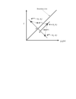
Figure 4: One exchange step in projection of a source $\mbox{\boldmath$\theta$}^{\prime}\in\Lambda_{k}$ onto the pattern space $\Psi\left(\Lambda_{k}\right)$

Now, using (64),

$$\left\|\mbox{\boldmath$\theta$}-\mbox{\boldmath$\theta$}^{\prime}\right\|^{2}-\left\|\mbox{\boldmath$\theta$}-\mbox{\boldmath$\psi$}\left(\mbox{\boldmath$\theta$}^{\prime}\right)\right\|^{2} = \sum_{l}\left\{\left\|\mbox{\boldmath$\theta$}-\mbox{\boldmath$\theta$}^{\prime(l-1)}\right\|^{2}-\left\|\mbox{\boldmath$\theta$}-\mbox{\boldmath$\theta$}^{\prime(l)}\right\|^{2}\right\}$$ (65)

$$= 2\sum_{l}\left(\theta^{\prime(l)}_{j_{l}}-\theta^{\prime(l)}_{i_{l}}\right)\left(\theta_{j_{l}}-\theta_{i_{l}}\right)\geq 0.$$

Since all components of the sum are non-negative, the sum is also non-negative. This concludes the proof of Lemma 6.2. $\Box$

From Lemma 6.2, if $\left\|\mbox{\boldmath$\theta$}-\hat{\mbox{\boldmath$\theta$}}\right\|\leq 1/\sqrt{n}^{1-\varepsilon}$, then also $\left\|\mbox{\boldmath$\theta$}-\mbox{\boldmath$\psi$}\left(\hat{\mbox{\boldmath$\theta$}}\right)\right\|\leq 1/\sqrt{n}^{1-\varepsilon}$. Similarly to the proof of Theorem 1, now let $\hat{\mbox{\boldmath$\theta$}}^{\psi}_{\Omega}$ be the point in the random pattern grid, denoted by $\Psi\left(\mbox{\boldmath$\Omega$}\right)$, nearest to $\mbox{\boldmath$\psi$}\left(\hat{\mbox{\boldmath$\theta$}}\right)$. Then, using Lemmas 6.1 and 6.2, the probability that a sequence generated by $\theta$ will appear by $\Psi\left(X^{n}\right)$ to have been generated by another source in the same grid is upper bounded, as $n\rightarrow\infty$, by

$$P_{\theta}\left(\hat{\mbox{\boldmath$\theta$}}^{\psi}_{\Omega}\neq\mbox{\boldmath$\theta$}\right)\leq P_{\theta}\left\{\left\|\mbox{\boldmath$\psi$}\left(\hat{\mbox{\boldmath$\theta$}}\right)-\mbox{\boldmath$\theta$}\right\|>\frac{1}{\sqrt{n}^{1-\varepsilon}}\right\}\leq P_{\theta}\left\{\left\|\hat{\mbox{\boldmath$\theta$}}-\mbox{\boldmath$\theta$}\right\|>\frac{1}{\sqrt{n}^{1-\varepsilon}}\right\}\rightarrow 0.$$ (66)

The first bound is since not all points in $\Psi\left(\mbox{\boldmath$\Omega$}\right)$ are contained in spheres. Hence, distinguishability is attained. This concludes the proof of Theorem 2. $\Box$

7 Upper Bounds

We now show how to design codes that attain low redundancy for coding patterns induced by i.i.d. sequences. We propose a code with good performance for smaller alphabets sizes, namely, $k\leq\sqrt{n}^{1-\varepsilon}$, for an arbitrarily small $\varepsilon>0$, and combine it with the method in [20] to asymptotically achieve the better compression of the two for a specific pattern. The new code uses Rissanen’s [24] two-part grid based coding approach combined with a non-uniform grid that resembles that in Section 5. For a given sequence with $\hat{k}$ distinct symbols, we find the best $\hat{k}$-dimensional pattern probability vector $\widehat{\mbox{\boldmath$\psi$}\left(\mbox{\boldmath$\theta$}\right)}$, which is the vector that gives the $\hat{k}$th-order ML probability for the pattern of the sequence. Note that $\widehat{\mbox{\boldmath$\psi$}\left(\mbox{\boldmath$\theta$}\right)}$ may be different from $\hat{\mbox{\boldmath$\theta$}}$ and $\mbox{\boldmath$\psi$}\left(\hat{\mbox{\boldmath$\theta$}}\right)$. (Furthermore, the actual ML estimate of a pattern may contain more letters than those actually observed. However, in analyzing this code, we constrain the analysis to the average case, in which our reference is the $k$-dimensional pattern probability, and to the class $\tilde{\Lambda}_{k}$ in which it is unlikely that $\hat{k}<k$.) Then, $\widehat{\mbox{\boldmath$\psi$}\left(\mbox{\boldmath$\theta$}\right)}$ is quantized to a grid. The quantized components are first coded, and then, the sequence is assigned a probability according to these quantized probability parameters. In [20], the number of all different types of patterns of length $n$ is shown to equal the number of unordered partitioning of the integer $n$. Given the type, the pattern ML probability vector $\widehat{\mbox{\boldmath$\psi$}_{u}\left(\mbox{\boldmath$\theta$}\right)}$ can be computed, as well as its ML probability, which is used to then encode the sequence using a number of bits that equals its negative logarithm. Hence, the redundancy is the logarithm of the number of types, as shown in the upper bound of (23). The combined code can compute both description lengths, and then choose between them, and use the one that requires fewer bits. One bit is needed to relay to the decoder which of the codes is used. We summarize the performance of the code combined of both codes in the next theorem.

Theorem 3

Fix an arbitrarily small $\varepsilon>0$, and let $n\rightarrow\infty$. Then, there exist codes with length function $L^{*}\left(\cdot\right)$ that achieve redundancy

$$R_{n}\left[L^{*},\mbox{\boldmath$\psi$}\left(\mbox{\boldmath$\theta$}\right)\right]\leq\left\{\begin{array}[]{ll}\left(1+\varepsilon\right)\frac{k-1}{2n}\log\frac{n^{1+\varepsilon}}{k^{2}},&\mbox{for }k\leq\sqrt{n}^{1-\varepsilon}~{}\mbox{and}~{}\mbox{\boldmath$\theta$}\in\tilde{\Lambda}_{k}\\ \frac{\pi\sqrt{2/3}\log e}{\sqrt{n}}+O\left(\frac{1}{n}\right),&\mbox{for }k\geq\sqrt{n}^{1-\varepsilon}~{}\mbox{or}~{}\mbox{\boldmath$\theta$}\not\in\tilde{\Lambda}_{k}\end{array}\right.$$ (67)

for patterns induced by any i.i.d. source $\mbox{\boldmath$\theta$}\in\Lambda_{k}$, with alphabet of size $k$.

The first region of Theorem 3 applies to the class $\tilde{\Lambda}_{k}$, i.e., it is assumed that the probability that less than $k$ letters will be observed in $X^{n}$ is $o(k/n)$. If the probabilities of all letters are greater than $1/n^{1-\varepsilon}$, this condition is satisfied. Note that the proposed code should also achieve good performance even if less than $k$ letters are likely to be observed in $X^{n}$. However, further research still needs to guarantee that the penalty does not increase in this case, and is still bounded as in the first region of (67). The bound of the first region of (67) also applies to the individual pattern redundancy under the assumption that the underlying alphabet contains no symbols other than those observed. A weaker upper bound, which is to first order twice the bound of the first region of (67) was subsequently derived in [21] for coding individual patterns with $k$ occurring indices as long as $k=o\left(n^{1/3}\right)$. While the bound in [21] is larger (thus weaker) and applies only to smaller $k$’s, it is stronger in the sense that it applies to a wider class containing all sequences in which $k$ symbols occur, without restricting the pattern generating alphabet to contain only symbols observed in $X^{n}$. The bound in the second region of Theorem 3 applies to the class $\Lambda_{k}$.

The upper bounds in (67) show that we can design universal codes for patterns that require at most $0.5\log(n/k^{2})$ bits for each unknown probability parameter, as long as $k$ is small enough, essentially of $O\left(\sqrt{n}\right)$ or less. If $k$ is larger, we observe a similar phenomenon as that of the lower bounds, in which we achieve the same redundancy for every large $k$, which is of $O\left(n^{-1/2}\right)$ bits per symbol overall. This performance is better than that attainable in standard i.i.d. compression. In particular, in the first region we gain $0.5\log k$ bits for each parameter, and the gain increases with $k$ in the second region. In Section 9, we discuss a different method that can be used to bound the redundancy in the second region. The ideas considered can be used (as in subsequent work [35]) to obtain stronger bounds in this region.

As indicated earlier, we observe gaps between the upper bounds and the lower bounds considered in the previous sections. In the first region, the lower bound is smaller by $0.5\log k$ bits for each parameter, whereas in the second region (as in the results in [17]-[21]), the lower bound is of $O\left(n^{-2/3}\right)$ overall instead of $O\left(n^{-1/2}\right)$. Naturally, the second region for the lower bounds starts with smaller $k$. Gaps between the upper and the lower bounds are still an open problem and will be discussed in Section 9 in somewhat more detail. This section is concluded with the proof of Theorem 3.

Proof of Theorem 3: To prove Theorem 3, we demonstrate and analyze the code that achieves the redundancy bound for the first region of (67). As mentioned earlier, a given pattern is encoded by this code as well as the code in [20], and the one with the smaller description length is then chosen. One bit is used to convey which code has been used (resulting in the additional $O(1/n)$ term of the second region). The rest of the proof is thus focused on the first region and bounding the performance of the new code. The proof for the second region is concluded using [20].

Using the code for the first region, we first need $\left(1+\varepsilon\right)\log\hat{k}$ bits to encode the number of occurring letters $\hat{k}$ with Elias’s coding for the integers [8]. Let $\mbox{\boldmath$\theta$}\in\tilde{\Lambda}_{k}$ and $k\leq\sqrt{n}^{1-\varepsilon}$. Let $\widehat{\mbox{\boldmath$\psi$}\left(\mbox{\boldmath$\theta$}\right)}=\left(\psi_{1},\psi_{2},\ldots,\psi_{\hat{k}}\right)$ be the $\hat{k}$-dimensional probability vector that maximizes the probability of $\Psi\left(X^{n}\right)$ in (9) for $X^{n}$. Let $\hat{\mbox{\boldmath$\theta$}}$ be the i.i.d. ML estimator of $\theta$ from $X^{n}$. Let $\mbox{\boldmath$\tau$}\stackrel{{\scriptstyle\triangle}}{{=}}\left(\tau_{1},\tau_{2},\ldots,\tau_{b},\ldots,\tau_{B}\right)$ be a grid of $B$ points whose $b$th component is defined in a similar manner to (31), where $-\varepsilon$ is replaced by $\varepsilon$, i.e.,

$$\tau_{b}\stackrel{{\scriptstyle\triangle}}{{=}}\sum_{j=1}^{b}\frac{2(j-\frac{1}{2})}{n^{1+\varepsilon}}=\frac{b^{2}}{n^{1+\varepsilon}}.$$ (68)

Thus, there are

$$B=\sqrt{n}^{1+\varepsilon}$$ (69)

points in $\tau$. Let $\mbox{\boldmath$\varphi$}\stackrel{{\scriptstyle\triangle}}{{=}}\left(\varphi_{1},\varphi_{2},\ldots,\varphi_{k-1},\varphi_{k}\right)$ be a quantized version of $\widehat{\mbox{\boldmath$\psi$}\left(\mbox{\boldmath$\theta$}\right)}$, for which each of the first $k-1$ components $\varphi_{i}$ takes one of the two nearest grid points surrounding $\psi_{i}$, i.e., if $\psi_{i}\in\left[\tau_{b},\tau_{b+1}\right]$, $\varphi_{i}$ equals either $\tau_{b}$ or $\tau_{b+1}$. The point that is chosen for $\varphi_{i}$ between the two grid points is the one that minimizes the absolute value of the cumulative difference between the first $k-1$ components of $\widehat{\mbox{\boldmath$\psi$}\left(\mbox{\boldmath$\theta$}\right)}$ and those of $\varphi$ such that the non-decreasing order of the components of $\varphi$ is retained. This ensures that the last largest component $\varphi_{k}$ of $\varphi$ is within the defined grid spacing around $\psi_{k}$, even if it does not take a value in $\tau$.

The code first codes the first $k-1$ components of $\varphi$, and then computes $P_{\varphi}\left[\Psi\left(X^{n}\right)\right]$, and uses (up to integer length constraints) $-\log P_{\varphi}\left[\Psi\left(X^{n}\right)\right]$ bits to code the pattern. The average code length for $\mbox{\boldmath$\theta$}\in\tilde{\Lambda}_{k}$ and $k\leq\sqrt{n}^{1-\varepsilon}$ is thus bounded (up to integer length constraints) by

$$E_{\theta}L^{*}\left[\Psi\left(X^{n}\right)\right]\leq 1+\left(1+\varepsilon\right)\log k+E_{\theta}\left\{L^{*}_{R}\left[\widehat{\mbox{\boldmath$\psi$}\left(\mbox{\boldmath$\theta$}\right)}\right]\right\}-E_{\theta}\left\{\log P_{\varphi}\left[\Psi\left(X^{n}\right)\right]\right\},$$ (70)

where $L^{*}_{R}\left[\widehat{\mbox{\boldmath$\psi$}\left(\mbox{\boldmath$\theta$}\right)}\right]$ is the cost of representing the quantized version $\varphi$ of $\widehat{\mbox{\boldmath$\psi$}\left(\mbox{\boldmath$\theta$}\right)}$. The first term of $1$ is the cost of one bit distinguishing between the two codes. The second term is a bound on the cost of representing $\hat{k}<k$. The last term is the cost of coding the pattern using the quantized ML estimates in $\varphi$. The inequality is also since some patterns may be represented shorter by the code from [20]. Denoting an upper bound on the representation cost of an up to $k$-dimensional vector $\varphi$ by $\bar{L}^{*}_{R,k}$, the average redundancy for $\mbox{\boldmath$\theta$}\in\tilde{\Lambda}_{k}$ and $k\leq\sqrt{n}^{1-\varepsilon}$ is, therefore, upper bounded by

$$nR_{n}\left[L^{*},\mbox{\boldmath$\psi$}\left(\mbox{\boldmath$\theta$}\right)\right] \leq 1+\left(1+\varepsilon\right)\log k+E_{\theta}\left\{L^{*}_{R}\left[\widehat{\mbox{\boldmath$\psi$}\left(\mbox{\boldmath$\theta$}\right)}\right]\right\}+E_{\theta}\left\{\log\frac{P_{\theta}\left[\Psi\left(X^{n}\right)\right]}{P_{\varphi}\left[\Psi\left(X^{n}\right)\right]}\right\}$$ (71)

$$\leq 1+\left(1+\varepsilon\right)\log k+\bar{L}^{*}_{R,k}+P_{\theta}\left(\hat{k}<k\right)n\log k+E_{\theta}\left\{\left.\log\frac{P_{\widehat{\psi\left(\theta\right)}}\left[\Psi\left(X^{n}\right)\right]}{P_{\varphi}\left[\Psi\left(X^{n}\right)\right]}\right|\hat{k}=k\right\}$$

$$= \bar{L}^{*}_{R,k}+E_{\theta}\left\{\left.\log\frac{P_{\widehat{\psi\left(\theta\right)}}\left[\Psi\left(X^{n}\right)\right]}{P_{\varphi}\left[\Psi\left(X^{n}\right)\right]}\right|\hat{k}=k\right\}+o\left(k\log\frac{n}{k^{2}}\right).$$

The second inequality is since at most $\log k$ bits are required to code every index, and also because the pattern probability w.r.t. the $k$-dimensional ML estimate is not smaller than the probability w.r.t. the actual parameter $\theta$. The next equality is because of the assumption that $P_{\theta}\left(\hat{k}<k\right)=o(k/n)$, and since $o\left(\log k\right)=o\left(\log(n/k^{2})\right)$ by definition of the region.

To complete the bound in the first region, we now need to bound the remaining first two terms of (71). These two costs are the cost of coding $\varphi$, and the cost of using the quantized version $\varphi$ of the $k$-dimensional pattern ML probability estimator $\widehat{\mbox{\boldmath$\psi$}\left(\mbox{\boldmath$\theta$}\right)}$ instead of using the actual $k$-dimensional pattern ML probability estimator. For the remainder of the proof, we can now assume that $\hat{k}=k$ because for the first term, we will obtain a bound that increases with $\hat{k}$, and for the second term, we compute the expectation conditioned on this event. We next bound the two costs and show that the second is negligible w.r.t. the first in the first region of the bound. This together with (71) results in the upper bound for this region.

Instead of coding the first $k-1$ components $\varphi_{i}$ of $\varphi$, we can code their indices in $\tau$. Let $b\left(\varphi_{i}\right)$ be the index in $\tau$ of the grid point that equals $\varphi_{i}$. Since the vector $\varphi$ is ordered, we can use a differential code which uses

$$\left(1+\varepsilon^{\prime}\right)\log\left[b\left(\varphi_{i}\right)-b\left(\varphi_{i-1}\right)+c\right]$$

bits, where $c$ is a constant, to represent the integer displacement to the index of $\varphi_{i}$ from that of $\varphi_{i-1}$ with Elias’s code, where $\varepsilon^{\prime}>0$ is arbitrarily small, $b\left(\varphi_{0}\right)\stackrel{{\scriptstyle\triangle}}{{=}}0$, and extra $c$ bits are added to apply for zero or small displacements. Hence, altogether, we will need

$$L^{*}_{R}\left[\widehat{\mbox{\boldmath$\psi$}\left(\mbox{\boldmath$\theta$}\right)}\right] = \sum_{i=1}^{k-1}\left(1+\varepsilon^{\prime}\right)\log\left[b\left(\varphi_{i}\right)-b\left(\varphi_{i-1}\right)+c\right]$$ (72)

$$\leq \left(1+\varepsilon^{\prime}\right)\left(k-1\right)\log\frac{B+ck}{k-1}$$

$$\leq \left(1+\varepsilon_{1}\right)\frac{k-1}{2}\log\frac{n^{1+\varepsilon}}{k^{2}}\stackrel{{\scriptstyle\triangle}}{{=}}\bar{L}^{*}_{R,k}$$

bits to represent $\varphi$, where the first inequality is obtained by Jensen’s inequality, and the second follows directly from (69) and the assumption that $k=o\left(\sqrt{n}\right)$ by absorbing low-order terms in $\varepsilon_{1}$. Note that the last inequality in (72) holds only for $k=o\left(\sqrt{n}\right)$. The bound of (72) is used to bound the cost of representing $\varphi$ in (71). (We note that in Section 9, we will demonstrate a method that yields representation cost for $\varphi$ which is fixed at $O\left(n^{(1+\varepsilon)/3}\right)$ bits. For $k\geq n^{1/3}$, this cost is better than that in (72). However, the cost of quantizing the pattern ML estimator, which is shown next, will overwhelm this cost for large $k$.)

We now bound the second term of (71). The probability of $\Psi\left(x^{n}\right)$ can be expressed as in (9) by summing over all sequences that have the same pattern with a fixed parameter vector. On the other hand, we can express the same probability by fixing the actual sequence and summing over all permutations of the parameter vector

$$P_{\theta}\left[\Psi\left(x^{n}\right)\right]=\sum_{\mbox{\boldmath$\sigma$}}P_{\theta(\sigma)}\left(x^{n}\right).$$ (73)

Now, to bound the cost of quantizing the pattern ML estimator reflected in the second term of (71), we consider the logarithm of the ratio between $P_{\widehat{\psi\left(\theta\right)}}\left[\Psi\left(X^{n}\right)\right]$ and $P_{\varphi}\left[\Psi\left(X^{n}\right)\right]$. We can express each of the two probabilities using (73). Then, we discard permutations of $\widehat{\psi\left(\theta\right)}$ that give negligible probability for $X^{n}$ (and their respective quantized versions) from each of the sums in the ratio. Next, we bound the ratio between the probability of $X^{n}$ given a non-negligible permutation of $\widehat{\psi\left(\theta\right)}$ and that obtained by the quantized version of this permutation. We obtain the same bound for all these permutations. This bound can, in turn, be used to bound the ratio between $P_{\widehat{\psi\left(\theta\right)}}\left[\Psi\left(X^{n}\right)\right]$ and $P_{\varphi}\left[\Psi\left(X^{n}\right)\right]$. To obtain the bound for all permutations, we need to bound the absolute differences between $\psi_{i}$ and $\varphi_{i}$, and between $\hat{\theta}_{i}$ and $\varphi(\sigma_{i})$, which is the $\sigma_{i}$th component of the permutation of $\varphi$ according to permutation vector $\sigma$. The first difference is a direct result of the definition of the components of $\tau$ in (68). The second difference is the reason we need to omit negligible permutations of $\widehat{\psi\left(\theta\right)}$ from the analysis. If we do not omit such permutations, we will be unable to bound this difference. Lemma 7.1, which is presented next, demonstrates that if the distance of components of a permutation of $\widehat{\psi\left(\theta\right)}$ from the respective non-permuted components of $\hat{\mbox{\boldmath$\theta$}}$ is too large, then the contribution of the conditional probability of this permutation to the probability of the pattern of $X^{n}$ in (73) will be negligible. A corollary to the lemma (which is shown in Appendix E as part of the proof of Lemma 7.2) will give us a bound on the absolute difference between components of a non-negligible permuted version of $\widehat{\psi\left(\theta\right)}$ and those of $\hat{\mbox{\boldmath$\theta$}}$, which, in turn, will lead to a bound on the desired difference between $\hat{\theta}_{i}$ and $\varphi(\sigma_{i})$.

We begin by showing that there are permutations of the pattern ML estimator that contribute negligibly to the pattern probability. The following lemma can be used to demonstrate that. The lemma is stated more generally.

Lemma 7.1

Let $n\rightarrow\infty$. Let $\hat{\mbox{\boldmath$\theta$}}$ be the standard i.i.d. ML estimator with $k$ non-zero components of the probability vector that governs $X^{n}$. Let $\mbox{\boldmath$\phi$}\stackrel{{\scriptstyle\triangle}}{{=}}\left(\phi_{1},\phi_{2},\ldots,\phi_{k}\right)$ be another $k$-dimensional probability vector. Define

$$\delta_{i}\stackrel{{\scriptstyle\triangle}}{{=}}\hat{\theta}_{i}-\phi_{i},~{}~{}i=1,2,\ldots,k.$$ (74)

Assume that there exists a set $J$ of at least $j$ indices $i\in J$, $1\leq i\leq k$, such that

$$\left|\delta_{i}\right|\geq\left\{\begin{array}[]{ll}\frac{k}{j}\cdot\frac{\sqrt{\hat{\theta}_{i}}}{\sqrt{n}^{1-\varepsilon/4}};&\mbox{if}~{}\phi_{i}>2\hat{\theta}_{i},\\ \sqrt{\frac{k}{j}}\cdot\frac{\sqrt{\hat{\theta}_{i}}}{\sqrt{n}^{1-\varepsilon/4}};&\mbox{if}~{}\phi_{i}\leq 2\hat{\theta}_{i}.\end{array}\right.$$ (75)

Then, as $n\rightarrow\infty$,

$$\frac{k!P_{\phi}\left(X^{n}\right)}{P_{\hat{\theta}}\left(X^{n}\right)}\rightarrow 0.$$ (76)

Lemma 7.1 shows that if there are too many components of a vector $\phi$ that are far from those of $\hat{\mbox{\boldmath$\theta$}}$, then even if we multiply the probability of $X^{n}$ given $\phi$ by $k!$ it still remains negligible w.r.t. the ML probability of $X^{n}$. The lemma shows that this is true for large distance with few components, as well as smaller distance with more components. Lemma 7.1 is proved in Appendix D.

For the sake of simple notation, let $\mbox{\boldmath$\psi$}\stackrel{{\scriptstyle\triangle}}{{=}}\widehat{\mbox{\boldmath$\psi$}\left(\mbox{\boldmath$\theta$}\right)}$ denote the pattern ML probability parameter vector from this point on to the end of the proof of the redundancy of the code for the first region. (This is a slight abuse of notation, but is much less tedious.) Now, $\mbox{\boldmath$\psi$}\left(\mbox{\boldmath$\sigma$}\right)$ and $\mbox{\boldmath$\varphi$}\left(\mbox{\boldmath$\sigma$}\right)$ are the permutations of $\psi$ and $\varphi$, respectively, obtained by permutation vector $\sigma$. Define the set ${\cal A}$ as the set of all permutation vectors $\sigma$, for which $\mbox{\boldmath$\phi$}\stackrel{{\scriptstyle\triangle}}{{=}}\mbox{\boldmath$\psi$}(\mbox{\boldmath$\sigma$})$ satisfies the condition in Lemma 7.1 w.r.t. $\hat{\mbox{\boldmath$\theta$}}$. Note that Lemma 7.1 also implies that $\psi$ cannot satisfy its conditions w.r.t. $\hat{\mbox{\boldmath$\theta$}}$. Then, given that for every $\mbox{\boldmath$\psi$}(\mbox{\boldmath$\sigma$})\not\in{\cal A}$, we obtain $P_{\psi\left(\sigma\right)}\left(X^{n}\right)/P_{\varphi\left(\sigma\right)}\left(X^{n}\right)\leq\alpha$, for some expression $\alpha$, the normalized contribution of the quantization of $\psi$ to the redundancy for every $x^{n}$ with $\hat{k}=k\leq\sqrt{n}^{1-\varepsilon}$ observed symbols can be upper bounded by

$$\frac{1}{n}\log\frac{P_{\widehat{\psi(\theta)}}\left[\Psi\left(x^{n}\right)\right]}{P_{\varphi}\left[\Psi\left(x^{n}\right)\right]} = \frac{1}{n}\log\frac{\sum_{\mbox{\boldmath$\sigma$}}P_{\psi(\sigma)}\left(x^{n}\right)}{\sum_{\mbox{\boldmath$\sigma$}}P_{\varphi(\sigma)}\left(x^{n}\right)}$$ (77)

$$= \frac{1}{n}\log\frac{\sum_{\mbox{\boldmath$\sigma$}:\mbox{\boldmath$\psi$}(\mbox{\boldmath$\sigma$})\not\in{\cal A}}P_{\psi(\sigma)}\left(x^{n}\right)+\sum_{\mbox{\boldmath$\sigma$}:\mbox{\boldmath$\psi$}(\mbox{\boldmath$\sigma$})\in{\cal A}}P_{\psi(\sigma)}\left(x^{n}\right)}{\sum_{\mbox{\boldmath$\sigma$}:\mbox{\boldmath$\psi$}(\mbox{\boldmath$\sigma$})\not\in{\cal A}}P_{\varphi(\sigma)}\left(x^{n}\right)+\sum_{\mbox{\boldmath$\sigma$}:\mbox{\boldmath$\psi$}(\mbox{\boldmath$\sigma$})\in{\cal A}}P_{\varphi(\sigma)}\left(x^{n}\right)}$$

$$\leq \frac{1}{n}\log\frac{\left(1+\varepsilon_{2}\right)\sum_{\mbox{\boldmath$\sigma$}:\mbox{\boldmath$\psi$}(\mbox{\boldmath$\sigma$})\not\in{\cal A}}P_{\psi(\sigma)}\left(x^{n}\right)}{\sum_{\mbox{\boldmath$\sigma$}:\mbox{\boldmath$\psi$}(\mbox{\boldmath$\sigma$})\not\in{\cal A}}P_{\varphi(\sigma)}\left(x^{n}\right)}$$

$$\leq \frac{1}{n}\log\frac{\left(1+\varepsilon_{2}\right)\sum_{\mbox{\boldmath$\sigma$}:\mbox{\boldmath$\psi$}(\mbox{\boldmath$\sigma$})\not\in{\cal A}}\alpha P_{\varphi(\sigma)}\left(x^{n}\right)}{\sum_{\mbox{\boldmath$\sigma$}:\mbox{\boldmath$\psi$}(\mbox{\boldmath$\sigma$})\not\in{\cal A}}P_{\varphi(\sigma)}\left(x^{n}\right)}~{}\leq~{}\frac{\varepsilon_{2}\log e}{n}+\frac{\log\alpha}{n}.$$

The first inequality is obtained from Lemma 7.1, using a fixed arbitrarily small $\varepsilon_{2}>0$, and also by decreasing the denominator. The last inequality is obtained since $\ln\left(1+x\right)\leq x$ for every $x>-1$. To complete the bound, we need to find $\alpha$. This is done in the following lemma.

Lemma 7.2

Let $\psi$ be the $k$-dimensional pattern ML estimator obtained from $X^{n}$ for $k\leq\sqrt{n}^{1-\varepsilon}$, let $\varphi$ be its quantized version, and let $\sigma$ be a permutation vector such that $\mbox{\boldmath$\psi$}(\mbox{\boldmath$\sigma$})\not\in{\cal A}$. Then,

$$\log\frac{P_{\psi(\sigma)}\left(X^{n}\right)}{P_{\varphi(\sigma)}\left(X^{n}\right)}\leq\frac{ck\ln k}{n^{\varepsilon/4}},$$ (78)

where $c$ is a constant.

The proof of Lemma 7.2 is in Appendix E. We can plug (78) in (77) for a particular $x^{n}$ to show that

$$\frac{1}{n}\log\frac{P_{\widehat{\psi(\theta)}}\left[\Psi\left(x^{n}\right)\right]}{P_{\varphi}\left[\Psi\left(x^{n}\right)\right]}\leq\frac{\varepsilon_{2}\log e}{n}+\frac{ck\ln k}{n^{1+\varepsilon/4}}=o\left(\frac{k}{n}\right),$$ (79)

and hence the quantization cost is negligible w.r.t. the cost of representing $\varphi$ in (72). Plugging the bounds of (72) and (79) in (71), absorbing all low order terms in the leading $\varepsilon$, normalizing by $n$, we obtain the upper bound of the first region of (67), thus concluding the proof of Theorem 3. $\Box$

8 Low Complexity Sequential Schemes and Pattern Entropy

We now present two sub-optimal low-complexity sequential algorithms for compressing patterns. We are interested in analyzing the performance for various alphabet sizes, and in the total description length of a pattern, which can be obtained by adding the modified redundancy we obtain here to the i.i.d. entropy as in (15). The results in this section provide bounds on the universal description length for coding patterns. A very interesting corollary is that for sufficiently large alphabets, the universal description length of patterns is smaller than the i.i.d. entropy. This points out to an interesting phenomenon where the pattern entropy must decrease from the i.i.d. one for sufficiently large alphabets. Subsequently to the work reported in this paper, pattern entropy and entropy rate have been extensively studied, first in [34], and later in [11]-[12], [22]-[23], [31], [38]-[39].

8.1 Known Alphabet Size and A Mixture Code

Let us first assume that although the alphabet $\Sigma$ itself is unknown, its size $k$ is known. For coding i.i.d. sequences, Krichevsky and Trofimov [15] demonstrated that the minimum description length (MDL) for i.i.d. sequences [24], [30] can be sequentially achieved using sequential probability assignment, which when combined with arithmetic coding [25] results in an optimal sequential code. In particular, they defined the probability $Q_{KT}\left(x^{n}\right)$ which is sequentially assigned to the sequence $x^{n}$ as

$$Q_{KT}\left(x^{n}\right)=\prod_{i=1}^{n}Q_{KT}\left(x_{i}~{}|~{}x^{i-1}\right),$$ (80)

where $Q_{KT}\left(x_{i}~{}|~{}x^{i-1}\right)$ is a conditional probability assigned to the $i$th symbol $x_{i}$, given the subsequence of all the preceding symbols $x^{i-1}$. It is defined as

$$Q_{KT}\left(x_{i}~{}|~{}x^{i-1}\right)\stackrel{{\scriptstyle\triangle}}{{=}}\frac{n^{i-1}\left(x_{i}\right)+1/2}{i-1+k/2},$$ (81)

where $n^{i-1}\left(x_{i}\right)$ is the number of occurrences of the symbol $x_{i}$ in the subsequence $x^{i-1}$.

We can adopt this approach for coding patterns if we know that $k$ symbols occur in the sequence. If a letter (or index) has already occurred, we can still update the probability as in (81). However, once a new symbol occurs, i.e., $x_{i}$ is not contained in the subsequence $x^{i-1}$, $\Psi\left(x_{i}\right)$ will be determined as the next available index, regardless of the actual value of $x_{i}$. This means that the event that $\Psi\left(x_{i}\right)$ will take a new value not in $\Psi\left(x^{i-1}\right)$ should be assigned the sum of the probabilities of all letters $u\in\Sigma$ that have not yet occurred. Hence, similarly to (80), $\Psi\left(x^{n}\right)$ will be assigned probability

$$Q_{k}\left[\Psi\left(x^{n}\right)\right]=\prod_{i=1}^{n}Q_{k}\left[\Psi\left(x_{i}\right)~{}|~{}x^{i-1}\right],$$ (82)

where

$$Q_{k}\left[\Psi\left(x_{i}\right)~{}|~{}x^{i-1}\right]=\left\{\begin{array}[]{ll}\frac{n^{i-1}\left(x_{i}\right)+1/2}{i-1+k/2},&\mbox{if~{}}n^{i-1}\left(x_{i}\right)>0,\\ \frac{\left(k-C_{i-1}\right)/2}{i-1+k/2},&\mbox{otherwise},\end{array}\right.$$ (83)

where $C_{i-1}$ is the number of distinct letters that occurred in the subsequence $x^{i-1}$. Theorem 4 summarizes the performance of the probability assignment in (82)-(83).

Theorem 4

Let $n\rightarrow\infty$. Then, the individual modified redundancy of the probability assignment in (82)-(83) is upper bounded by

$$\tilde{R}_{n}\left[Q_{k},\Psi\left(x^{n}\right)\right]\leq\frac{k}{2n}\log\frac{n}{k^{3}}+\left(\frac{19}{12}\log e\right)\frac{k}{n}-\frac{1}{2n}\log n+O\left(\frac{k^{2}}{n^{2}}\right).$$ (84)

for every pattern $\Psi\left(x^{n}\right)$ of a sequence $x^{n}$ with $k$ distinct indices and for every $k\leq n$.

The proof of Theorem 4 is purely technical relying on Stirling’s approximation and is presented in Appendix F. From the proof, we can see that the last term is $k^{2}(\log e)/\left(4n^{2}\right)$, which is always negligible w.r.t. the sum of all other terms. We can also notice from the proof that if almost all letters in $x^{n}$ (except $o(k)$) occur more than a fixed number of occurrences, (84) reduces to

$$\tilde{R}_{n}\left[Q_{k},\Psi\left(x^{n}\right)\right]\leq\frac{k}{2n}\log\frac{n}{k^{3}}+\left(1.5\log e\right)\frac{k}{n}-\frac{1}{2n}\log n+O\left(\frac{k^{2}}{n^{2}}\right),$$ (85)

for every $k$ (i.e., the second term is slightly smaller). However, if there are $O(k)$ letters that occur only one time, we must include the term of at most $k(\log e)/12$, obtained from the upper bound of Stirling’s approximation. Worst sequence case bounds on the individual true redundancy can be easily obtained from Theorem 4. If the alphabet size is limited to $k$, the pattern probability of the worst sequence will be at most $k!$ times its i.i.d. ML probability. Hence, the redundancy will increase by $\log(k!)$, yielding the same redundancy as that of the i.i.d. case of $0.5(k-1)\log(n/k)$ bits, which diminishes for $k=o(n)$.

The expression in (85) attains a maximum for $k=n^{1/3}$ (neglecting the last two terms). The maximum of (85) meets the performance of the minimax code in (22). In fact, a minimax code that does not distinguish between different $k$’s adopts the worst case performance of $k=n^{1/3}$ for every value of $k$. For $k>e\cdot n^{1/3}$, $\tilde{R}_{n}\left[Q_{k},\Psi\left(x^{n}\right)\right]$ in (85) becomes negative. (This is also true for (84) for $k>e^{19/18}\cdot n^{1/3}$.) This means that the number of bits required to code the pattern is smaller than the negative logarithm of the ML i.i.d. probability of $x^{n}$, and that the pattern entropy is much smaller than that of i.i.d. sequences for large $k$’s. This result cannot be observed from the lower and upper bounds of the previous sections because they refer to the true redundancy w.r.t. the pattern entropy. Further study of pattern entropy [31] extensively characterized the behavior of the pattern entropy for different alphabet sizes and arrangements of the letter probabilities in $\theta$.

The main drawback of the code above is that it requires knowledge of $k$. A “semi-sequential” two pass code that identifies $k$ during the first pass can be used to achieve almost similar performance with additional $(1+\varepsilon)\log k$ bits to inform the decoder of $k$. Elias’s coding of the integers [8] can be used to first encode $k$, and then the scheme of (82)-(83) is used to code the pattern. To avoid the use of a two pass code, one can perform a mixture over all possible values $j$ of $k$. This can be done by assigning at every $i$; $1\leq i\leq n$,

$$Q\left[\Psi\left(x^{i}\right)\right]\stackrel{{\scriptstyle\triangle}}{{=}}\frac{1}{n-1}\sum_{j=2}^{n}\tilde{Q}_{j}\left[\Psi\left(x^{i}\right)\right],$$ (86)

where $\tilde{Q}_{j}\left[\Psi\left(x^{n}\right)\right]$ is defined by

$$\tilde{Q}_{j}\left[\Psi\left(x_{i}\right)~{}|~{}x^{i-1}\right]\stackrel{{\scriptstyle\triangle}}{{=}}\left\{\begin{array}[]{ll}\frac{n^{i-1}\left(x_{i}\right)+1/2}{i-1+j/2},&\mbox{if}~{}j>C_{i-1}~{}\mbox{and}~{}n^{i-1}\left(x_{i}\right)>0,\\ \frac{\left(j-C_{i-1}\right)/2}{i-1+j/2},&\mbox{if~{}}j>C_{i-1}~{}\mbox{and}~{}n^{i-1}\left(x_{i}\right)=0,\\ \frac{1}{C_{i-1}+1},&\mbox{if}~{}j\leq C_{i-1},\end{array}\right.$$ (87)

i.e., as long as the number of distinct occurring letters does not exceed $j-1$, $\tilde{Q}_{j}\left[\Psi\left(x^{i}\right)\right]$ is equal to $Q_{j}\left[\Psi\left(x^{i}\right)\right]$. Otherwise, $\tilde{Q}_{j}\left[\Psi\left(x^{i}\right)\right]$ assigns equal probability to all existing indices and also to the innovation index. Then, $Q\left[\Psi\left(x^{i}\right)\right]$ is averaged over $\tilde{Q}_{j}\left[\Psi\left(x^{i}\right)\right]$. The assigned probability satisfies for the actual $k$,

$$Q\left[\Psi\left(x^{n}\right)\right]\geq\frac{1}{n}Q_{k+1}\left[\Psi\left(x^{n}\right)\right],$$ (88)

where we must consider index $k+1$ in case all $k$ symbols occur first earlier than at time $n$. This leads to modified redundancy of

$$\tilde{R}_{n}\left[Q,\Psi\left(x^{n}\right)\right]\leq\frac{k}{2n}\log\frac{n}{k^{3}}+\left(\frac{19}{12}\log e\right)\frac{k}{n}+\frac{1}{2n}\log\frac{n^{2}}{k^{3}}+O\left(\frac{k^{2}}{n^{2}}\right),$$ (89)

where the third term diverges from (84) because of the mixing and the use of $k+1$ instead of $k$, for this linear per-symbol complexity scheme.

8.2 Unknown Alphabet Size

The assignment described requires extra manipulations or complexity for an unknown $k$. In [41], a more generalized form of (81) was presented, in which

$$Q_{GKT}\left(x_{i}~{}|~{}x^{i-1}\right)\stackrel{{\scriptstyle\triangle}}{{=}}\left\{\begin{array}[]{ll}\frac{n^{i-1}\left(x_{i}\right)+\nu}{i-1+C_{i-1}\nu+\chi_{i-1}},&\mbox{if~{}}n^{i-1}\left(x_{i}\right)>0,\\ \frac{\chi_{i-1}}{\left(M-C_{i-1}\right)\left(i-1+C_{i-1}\nu+\chi_{i-1}\right)},&\mbox{otherwise}\end{array}\right.,$$ (90)

where $\nu>0$ is some constant, $\chi_{i-1}$ is some function of the subsequence $x^{i-1}$, and $M$ is a bound on the maximum number of alphabet letters. This extension of (81) allows asymptotically optimal performance for coding i.i.d. sequences. This performance depends only on the actual number $k$ of alphabet letters that occur, and not on the total alphabet size $M$.

It turns out that with correct modification of (90), one can sequentially (with fixed per symbol complexity) asymptotically (with $k\rightarrow\infty$) achieve the same performance of (84)-(85) for patterns. Let us consider the code in which

$$Q\left[\Psi\left(x_{i}\right)~{}|~{}x^{i-1}\right]\stackrel{{\scriptstyle\triangle}}{{=}}\left\{\begin{array}[]{ll}\frac{n^{i-1}\left(x_{i}\right)+1/2}{i-1+C_{i-1}/2+\left(C_{i-1}+1\right)^{1-\varepsilon}/2},&\mbox{if~{}}n^{i-1}\left(x_{i}\right)>0,\\ \frac{\left(C_{i-1}+1\right)^{1-\varepsilon}/2}{i-1+C_{i-1}/2+\left(C_{i-1}+1\right)^{1-\varepsilon}/2},&\mbox{otherwise},\end{array}\right.$$ (91)

where $\varepsilon>0$ can be chosen arbitrarily small. Theorem 5 summarizes the performance of this code.

Theorem 5

Let $n\rightarrow\infty$. Then, the individual modified redundancy of the probability assignment in (91) is upper bounded by

$$\tilde{R}_{n}\left[Q,\Psi\left(x^{n}\right)\right] \leq \frac{k}{2n}\log\frac{n}{k^{3}}+\left(\frac{19}{12}-\varepsilon\right)\left(\log e\right)\frac{k}{n}-\frac{1}{2n}\log n+$$ (92)

$$\frac{k^{1-\varepsilon}}{2n}\log\frac{2n}{k}+\frac{\varepsilon k\log k}{n}+O\left(\frac{k^{2}}{n^{2}}\right),$$

for every pattern $\Psi\left(x^{n}\right)$ of a sequence $x^{n}$ with $k$ distinct indices and for every $k\leq n$.

The proof of Theorem 5, again, relies on Stirling’s approximation. It is presented in Appendix G. The bound in (92) is shown such that the first row contains the terms (up to $\varepsilon$) identical to the upper bound in (84). The second row contains the additional terms that increase the bound due to the reduced complexity. If $k\rightarrow\infty$ and $\varepsilon$ is arbitrarily small, the bound in (92) asymptotically meets the modified redundancy upper bound of (84), even if $k$ goes to infinity at a slower rate than $n$. However, for smaller $k$’s, the two terms in the bottom row increase the redundancy, and if $k>n^{1/3}$, work against the dominant negative first term. In practice, $k$ may be too small, and the gap between the redundancy of the first scheme in (84) and that of the second scheme in (92) will be noticed. A mixture of the assigned probability of the new scheme and of those for known small $k$’s in (82)-(83) can be used to achieve the performance of (84) for every $k$.

Under the assumption leading to (85), the worst case modified redundancy of the first scheme is obtained when $k=n^{1/3}$, where the extra number of bits required beyond $-\log P_{ML}\left(x^{n}\right)$ is linear in $k$. The additional terms of the redundancy of the second scheme shift the maximum redundancy to a larger value of $k$, yielding larger redundancy. For example, if $k\rightarrow\infty$, a value of $\varepsilon=0.1$ will attain the worst $k$ (under the assumption leading to (85)) at $k\approx n^{0.5/(1.5-\varepsilon)}=n^{0.5/1.4}\approx n^{0.357}$, which is larger than $n^{1/3}$. If $n$ is not as large, the maximal redundancy will be attained for finite $k$’s, and will increase w.r.t. $k$. For example, if $n=10^{6}$, and $\varepsilon=0.1$, the worst case $k$ is slightly above $k=400$, which is approximately $n^{0.44}$. Figure 5 shows the un-normalized modified redundancy bounds (in bits) of both schemes (using a second order term of $1.5(\log e)k/n$, and for the first scheme with a known $k$), as well as the individual modified redundancies obtained using the two proposed schemes for patterns of actual sequences $x^{n}$. The results are shown for $n=10^{6}$, for alphabets of sizes $k=2$ to $k=1000$, and for $\varepsilon=0.1$ in the second scheme. For the second scheme, the results are also shown for the worst possible sequence, i.e., the one that is used to obtain the bound of Theorem 5, in which all the $k$ letters occur in the first $k$ symbols of $x^{n}$. The figure shows that the bound in (85) is tight. As expected, the first scheme performs better than the second. The bound of (92) is loose because the proof of Theorem 5 makes a loose assumption in order to use Stirling’s bounds. The algorithm is thus much better than the bound in (92). Since the performance is for an individual sequence, the simulation curve for the second scheme is rather noisy. The reason is that the behavior varies depending on where in the sequence first occurrences are. Since each point is for a different individual sequence, the locations of the first occurrences vary. Figure 5 also verifies the worst values of $k$ mentioned above.

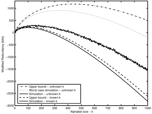
Figure 5: Bounds and simulation results for the individual modified pattern redundancies of two sequential schemes with $n=10^{6}$ and $\varepsilon=0.1$

For a given sequence $x^{n}$, the schemes described in this section assign probability based on only a single permutation of $\hat{\mbox{\boldmath$\theta$}}$. However, a pattern probability can be expressed as a sum of all permutations of its ML estimator. Naturally, if the probabilities of all $k!$ permutations are included in the assigned probability, better redundancy can be obtained. Subsequently to the derivation of the schemes described here, a class of computationally more demanding schemes that accounts to many such permutations was obtained and described in [18]-[20]. Unlike those schemes, the methods proposed here can more easily be integrated into efficient low-complexity implementations of adaptive arithmetic coding (see, e.g., [26]).

8.3 Pattern and I.I.D. Entropies

The description length in (84) can lead to an upper bound on the pattern entropy in terms of the i.i.d. one. In particular, it follows from (84), that if for an arbitrarily small $\varepsilon>0$, the probability that at least $k^{\prime}$ distinct symbols will occur in a sequence of length $n$ is at least $1-\varepsilon$, then

$$\frac{1}{n}H_{\theta}\left[\Psi\left(X^{n}\right)\right]\leq\left\{\begin{array}[]{ll}H_{\theta}\left(X\right);&\mbox{if}~{}k^{\prime}\leq e^{19/18}\cdot n^{1/3},\\ H_{\theta}\left(X\right)-\left(1-\varepsilon\right)\frac{3}{2}\frac{k^{\prime}}{n}\log\frac{k^{\prime}}{e^{19/18}n^{1/3}}+O\left(\frac{k^{\prime 2}+n\log n}{n^{2}}\right);&\mbox{if}~{}k^{\prime}>e^{19/18}\cdot n^{1/3}.\end{array}\right.$$ (93)

The last equation can be shown by bounding the entropy by the average description length of the following probability assignment code. The code assigns the pattern $\Psi\left(x^{n}\right)$ a codeword of length $-\log P_{\theta}\left[\Psi\left(x^{n}\right)\right]\leq-\log P_{\theta}\left(x^{n}\right)$ bits if less than $k^{\prime}$ indices occur in $\Psi\left(x^{n}\right)$. Otherwise, it uses the code leading to (84). One negligible bit is required to distinguish between the two cases, and at most $O(\log n)$ bits are needed to inform the decoder of the actual number of indices if greater than or equal $k^{\prime}$. Hence, for a large $k^{\prime}$, the pattern entropy is significantly smaller than the i.i.d. one. In fact, from (93) and the bounds derived in this paper, we observe that not only does the pattern entropy decrease significantly from the i.i.d. one, but also the true pattern redundancy becomes negligible compared to this decrease. The extensive study of the pattern entropy has been the subject of several subsequent works, first in [34], and later in [11]-[12], [22]-[23], [31], [38]-[39].

9 Discussion

This paper considered the average case of the problem of universal pattern compression. Both lower and upper bounds on the redundancies of codes for this problem were obtained. However, a gap still exists between the lower bounds and the attainable upper bounds. While we considered the average problem, other work [1], [13], [17]-[21] considered the individual sequence case, using different techniques based on combinatorics. Although the aim and the techniques in those independent works were different, similar qualitative results were obtained, and in particular the same gap was shown to exist between the orders of magnitudes of the lower and the upper bounds.

Future work should try to bridge the two sets of bounds. In our work, it is clear that there is room for improvement and tightening both lower and upper bounds. The minimax lower bounds derived in Section 5 are not tight because we decreased the grid size dividing by $k!$, which eliminated many permutations of $\mbox{\boldmath$\psi$}\left(\mbox{\boldmath$\theta$}\right)$, more than once each. In Section 6, the assumption that complete spheres are contained in the pattern space, and the division by their complete volume to find the number of spheres packed in the space resulted in a possibly loose bound for most sources. It may be possible to use techniques from combinatorics to tighten the bounds. The question is whether such techniques will improve the first order asymptotics or not.

On the other hand, the quantization approach of the upper bound in the first region may be useful also for the second region with larger $k$’s. The derivation of the upper bound of the second region does not quantize the estimators of the probability parameters, possibly leading to a loose bound. One can show that quantization of the ML parameters into the vector $\varphi$ whose components are on the grid points of $\tau$ defined in (68) can result in representation cost of $O\left(n^{(1+\varepsilon)/3}\right)$ even for large $k$’s. More precisely, let $\beta$ be some partitioning index in the grid $\tau$. Consider representing the quantized ML pattern probability parameters of $\varphi$ as follows: For each of the first $\beta$ grid points in $\tau$ use up to $(1+\varepsilon)\log k$ bits to represent how many letters have probabilities quantized in $\varphi$ to this grid point. In the remaining grid points (bounded by $B=\sqrt{n}^{1+\varepsilon}$) there are at most $n^{1+\varepsilon}/\beta^{2}$ quantized probability parameters in the components of $\varphi$ (see, e.g., (68)-(69)). For each of these components of $\varphi$, one can use up to $(1+\varepsilon)\log B$ bits to represent the index in $\tau$ of the point that equals this component. This results in a total representation cost upper bounded by

$$\left(1+\delta\right)\beta\log k+\left(1+\delta\right)\frac{n^{1+\varepsilon}}{2\beta^{2}}\log n$$ (94)

for some fixed $\delta>\varepsilon$. Differentiating w.r.t. $\beta$ to find the value of the partition point $\beta$ of $\tau$ that yields the minimum of the expression above yields a bound on the representation cost of

$$\left(1+\delta\right)1.5\cdot n^{\frac{1}{3}(1+\varepsilon)}\cdot\left(\log n\right)^{1/3}\cdot\left(\log k\right)^{2/3}$$ (95)

bits for coding $\varphi$. A more complex analysis takes the second cost above as the number of choices of at most $n^{1+\varepsilon}/\beta^{2}$ elements out of at most $\sqrt{n}^{1+\varepsilon}$ with repetitions allowed. Asymptotically, it yields the bound of (95) divided by a factor of $3^{1/3}$. Considering the bound only for $k\geq n^{1/3}$, this stronger bound can be bounded by $\left(1+\delta\right)1.5\cdot n^{\frac{1}{3}(1+\varepsilon)}\cdot\log k$.

From (95) we know that the representation of a quantized version of the pattern ML estimator whose components are quantized as proposed in Section 7 can cost $O\left(n^{(1+\varepsilon)/3}\right)$ bits for every $k$, including all large values of $k$ up to $k=n$. However, the quantization cost, in this case, increases and becomes of $O\left(k/n^{1+\varepsilon}\right)$ bits per symbol. While subsequent work in [35] has already improved the upper bound by trading off between the two costs, a gap to the lower bound still remains. Therefore, further research should explore this direction more in order to attempt to reduce the upper bound that consists of these two components even more.

10 Summary and Conclusions

We studied the average universal coding problem of patterns of sequences generated by i.i.d. sources. Lower bounds on the average minimax redundancy and the redundancy for most sources were obtained, as well as upper bounds obtained for specific codes. It was shown that for essentially small alphabet sizes, the redundancy cost in coding patterns is between $0.5\log(n/k^{3})$ and $0.5\log(n/k^{2})$ bits per each unknown probability parameter in all average senses. For essentially large alphabets, this cost is between $O\left(n^{1/3}\right)$ and $O\left(n^{1/2}\right)$ bits overall. These redundancies are better than those attained in standard i.i.d. sequence compression. In particular, for large $k$’s where universal compression with vanishing redundancy is impossible in the i.i.d. case, here it has vanishing redundancy. The gain over i.i.d. compression increases with $k$, since for large $k$’s, a fixed cost is maintained, regardless of the value of $k$. This gain is reflected even more in the existence of universal pattern codes whose pattern universal description length is smaller than the i.i.d. non-universal MDL of the underlying sequence if the alphabet is large enough. This implies a decrease of the pattern entropy w.r.t. the underlying i.i.d. one. This overall gain, of course, does not come for free, and the cost is embedded in coding the unknown alphabet characters before the patterns are obtained. Two low-complexity sub-optimal sequential algorithms were presented and were used to demonstrate the gain in coding patterns over the i.i.d. case. Future work should attempt to bridge the gap between the upper and lower bounds. Also, the results on the i.i.d. problem can serve as a basis for further research on pattern compression for patterns induced by non-memoryless sources.

Appendix Appendix A –   Proof of Lemma 5.1

The number of vectors ${\mathbf{b}}$ with integer components that satisfy (36) is lower bounded by the number of cubes with edge $1$ that are fully contained in the positive quadrant of the $k-1$ dimensional sphere centered at the origin with radius $\sqrt{n}^{1-\varepsilon}$. (This is a lower bound, because there are, in fact, more vectors with zero components than this number). The number of these cubes equals the total volume of these cubes. However, since there can exist cubes that are only partially contained in the sphere, the volume of the sphere with radius $\sqrt{n}^{1-\varepsilon}$ cannot be used to bound the total volume of these cubes. Instead, we can subtract the longest diagonal of these cubes $\sqrt{k-1}$ from the radius of the original sphere, and use the new sphere with radius $\sqrt{n}^{1-\varepsilon}-\sqrt{k-1}$ to bound the total volume of these cubes, or even use a shorter radius $\sqrt{n}^{1-\varepsilon^{\prime}}\leq\sqrt{n}^{1-\varepsilon}-\sqrt{k-1}$ for this bound (this radius is shorter by the assumption that $k\leq n^{1-2\varepsilon}\ll n^{1-\varepsilon}$). The volume of the positive quadrant of this sphere is bounded in (37). It is thus only left to show that all cubes that are only partially contained (or are not contained) in the sphere with radius $\sqrt{n}^{1-\varepsilon}$ are completely outside the sphere with radius $\sqrt{n}^{1-\varepsilon}-\sqrt{k-1}$. Hence, the volume of this sphere is a lower bound on the total volume of cubes for which the farthest points from the origin satisfy (36), and thus a lower bound on the number of integer components vectors ${\mathbf{b}}$ that satisfy this condition.

Let ${\mathbf{a}}\stackrel{{\scriptstyle\triangle}}{{=}}\left(a_{1},a_{2},\ldots,a_{k-1}\right)$ be the farthest point from the origin in an edge $1$ cube that is either partially in the sphere with radius $\sqrt{n}^{1-\varepsilon}$ centered at the origin or not in the sphere. By definition,

$$\sum_{i=1}^{k-1}a_{i}^{2}>n^{1-\varepsilon}~{}\Rightarrow~{}\sqrt{\sum_{i=1}^{k-1}a_{i}^{2}}>\sqrt{n}^{1-\varepsilon}~{}\Rightarrow~{}\frac{1}{\sqrt{n}^{1-\varepsilon}}>\frac{1}{\sqrt{\sum_{i=1}^{k-1}a_{i}^{2}}}.$$ (A.1)

By Jensen’s inequality on the function $x^{2}$,

$$\sum_{i=1}^{k-1}a_{i}^{2}\geq(k-1)\left(\sum_{i=1}^{k-1}\frac{a_{i}}{k-1}\right)^{2}=\frac{1}{k-1}\left(\sum_{i=1}^{k-1}a_{i}\right)^{2}~{}\Rightarrow~{}\sum_{i=1}^{k-1}a_{i}\leq\sqrt{k-1}\sqrt{\sum_{i=1}^{k-1}a_{i}^{2}}.$$ (A.2)

The nearest point to the origin of the cube considered is the point $\left(a_{1}-1,a_{2}-1,\ldots,a_{k-1}-1\right)$. To prove that the cube is completely outside the new sphere, we need to show that this nearest point to the origin is outside this sphere, i.e., that $\sum\left(a_{i}-1\right)^{2}>\rho^{2}$ where $\rho=\sqrt{n}^{1-\varepsilon}-\sqrt{k-1}$ is the radius of the new sphere. The difference between the two sides of this equation is

$$\sum_{i=1}^{k-1}\left(a_{i}-1\right)^{2}-\left(\sqrt{n}^{1-\varepsilon}-\sqrt{k-1}\right)^{2}=\left(\sum_{i=1}^{k-1}a_{i}^{2}-n^{1-\varepsilon}\right)-2\left(\sum_{i=1}^{k-1}a_{i}-\sqrt{k-1}\sqrt{n}^{1-\varepsilon}\right)$$ (A.3)

$$\geq \sqrt{n}^{1-\varepsilon}\left(\sqrt{\sum_{i=1}^{k-1}a_{i}^{2}}-\sqrt{n}^{1-\varepsilon}\right)-2\sqrt{k-1}\left(\sqrt{\sum_{i=1}^{k-1}a_{i}^{2}}-\sqrt{n}^{1-\varepsilon}\right)$$

$$= \left(\sqrt{n}^{1-\varepsilon}-2\sqrt{k-1}\right)\left(\sqrt{\sum_{i=1}^{k-1}a_{i}^{2}}-\sqrt{n}^{1-\varepsilon}\right)>0.$$

The first inequality is obtained by using (A.1) for the first term and (A.2) for the second. The next inequality is because the left term is positive as long as $k<n^{1-\varepsilon}/4+1$, and the right term is positive by (A.1). This proves that any point in a cube that is not completely inside the sphere with radius $\sqrt{n}^{1-\varepsilon}$ must be outside the sphere we defined with a smaller radius, and thus the volume of this sphere in the positive quadrant lower bounds the number of nonnegative integer components vectors that satisfy (36). This concludes the proof of Lemma 5.1. $\Box$

Appendix Appendix B –   Proof of Lemma 5.2

Let the observed data sequence $X^{n}$ be generated with distribution $P_{\theta}(x^{n})$, where $\mbox{\boldmath$\theta$}\in\mbox{\boldmath$\Omega$}$. Let $\hat{\mbox{\boldmath$\theta$}}$ be the ML estimate of $\theta$ from $X^{n}$. To bound the probability of event $A$, we will use the union bound on events $A_{i}$. Define

$$\delta_{i}\stackrel{{\scriptstyle\triangle}}{{=}}\hat{\theta}_{i}-\theta_{i}.$$ (B.1)

As defined in (41), event $A_{i}$ for $1\leq i\leq k$ occurs if $\left|\delta_{i}\right|\geq\Delta\left(\tau_{b_{i}}\right)/2$, where $\Delta\left(\tau_{b_{i}}\right)$ is as defined in (33). Recall that for $i<k$, $\tau_{b_{i}}=\theta_{i}$. For $i=k$, the constrained parameter $\theta_{k}$ may not be on $\tau$ and we define $\tau_{b_{k}}$ as the nearest point in $\tau$ to $\theta_{k}$ that is smaller than or equal to $\theta_{k}$. Note that in order to generate a bound that can be useful for the distinguishability of patterns, we must bound $P_{\theta}(A)$, which is greater than $P_{\theta}\left(\hat{\mbox{\boldmath$\theta$}}_{\Omega}\neq\mbox{\boldmath$\theta$}\right)$. The latter is sufficient for distinguishability in the i.i.d. case (see, e.g., [30]). In particular, we must include $A_{k}$ in the error event, although we can use the assumption that $\theta_{k}\geq\theta_{i}$, for all $i;1\leq i\leq k-1$. Hence, for all $i$, $\theta_{i}\geq 1/n^{1-\varepsilon}$ from the definition of the minimum grid point in (31).

In the following lemma, we lower bound $\left|\delta_{i}\right|$ as a function of $\hat{\theta}_{i}$ given event $A_{i}$ occurred. Following the lemma and its proof, we use this bound and the union bound on the components of $\theta$ to show that the overall probability of $A$ vanishes.

Lemma B.1

If event $A_{i}$ occurs, then event

$$B_{i}~{}:~{}\left|\delta_{i}\right|=\left|\hat{\theta}_{i}-\theta_{i}\right|\geq\frac{\sqrt{\hat{\theta}_{i}}}{10\sqrt{n}^{1-\varepsilon}}$$ (B.2)

must occur as well.

Note that if $\hat{\theta}_{i}=0$, Lemma B.1 holds simply because the right hand side of (B.2) is zero.

Proof: First, extend the definition of the function $\Delta\left(\theta\right)$, defined in (33), to every value of $\theta\geq 1/n^{1-\varepsilon}$,

$$\Delta\left(\theta\right)\stackrel{{\scriptstyle\triangle}}{{=}}\frac{2\left(\sqrt{\theta}\sqrt{n}^{1-\varepsilon}-0.5\right)}{n^{1-\varepsilon}}\geq\frac{\sqrt{\theta}}{\sqrt{n}^{1-\varepsilon}}.$$ (B.3)

The function $\Delta\left(\theta\right)$ is increasing in $\theta$. Now, given $A_{i}$ occurred, consider two separate cases: (1) $\hat{\theta}_{i}\leq\tau_{b_{i}+2}$, and (2) $\hat{\theta}_{i}>\tau_{b_{i}+2}$. For case (1),

$$\left|\delta_{i}\right|=\left|\hat{\theta}_{i}-\theta_{i}\right|\geq\frac{\Delta\left(\tau_{b_{i}}\right)}{2}\geq\frac{\Delta\left(\tau_{b_{i}+2}\right)}{10}\geq\frac{\sqrt{\tau_{b_{i}+2}}}{10\sqrt{n}^{1-\varepsilon}}\geq\frac{\sqrt{\hat{\theta}_{i}}}{10\sqrt{n}^{1-\varepsilon}}.$$ (B.4)

To obtain the second inequality, we use the fact that $\Delta\left(\tau_{b_{i}+2}\right)\leq 5\Delta\left(\tau_{b_{i}}\right)$, which can be shown by observing the case $b_{i}=1$. Then, inequality (B.3) is used. Finally, the definition of this case leads to the last inequality. (Note that we need to consider $\tau_{b_{i}+2}$ instead of $\tau_{b_{i}+1}$ only in case $\theta_{k}$ is closer to $\tau_{b_{k}+1}$ than to $\tau_{b_{k}}$, resulting in $\hat{\theta}_{k}>\tau_{b_{k}+1}$ still satisfying the complement event to $A_{k}$.) For case (2), let $\hat{b}_{i}$ be the index of the largest grid point still smaller than $\hat{\theta}_{i}$, i.e., $\hat{\theta}_{i}>\tau_{\hat{b}_{i}}$. Then, since there is more than one unit of grid spacing between $\theta_{i}$ and $\hat{\theta}_{i}$,

$$\left|\delta_{i}\right|=\hat{\theta}_{i}-\theta_{i}>\Delta\left(\tau_{\hat{b}_{i}}\right)=\frac{2\left(\hat{b}_{i}-\frac{1}{2}\right)}{n^{1-\varepsilon}}\geq\frac{\hat{b}_{i}+\frac{1}{2}}{n^{1-\varepsilon}}=\frac{\Delta\left(\tau_{\hat{b}_{i}+1}\right)}{2}\geq\frac{\Delta\left(\hat{\theta}_{i}\right)}{2}\geq\frac{\sqrt{\hat{\theta}_{i}}}{2\sqrt{n}^{1-\varepsilon}}.$$ (B.5)

The second inequality is obtained since $\hat{b}_{i}\geq 2$. This concludes the proof of Lemma B.1. $\Box$

Using Lemma B.1 and the union bound,

$$P_{\theta}\left(A\right)\leq\sum_{i=1}^{k}P_{\theta}\left(A_{i}\right)\leq\sum_{i=1}^{k}P_{\theta}\left(B_{i}\right),$$ (B.6)

and we need to bound $P_{\theta}\left(B_{i}\right)$. Consider the Bernoulli $n$-sequence ${\mathbf{Y}}_{i}$, whose $j$th symbol is defined by

$$Y_{ij}=\left\{\begin{array}[]{ll}1,&\mbox{if}~{}X_{j}=i\\ 0,&\mbox{otherwise}\end{array}\right.,$$ (B.7)

where $X_{j}$ is the $j$th symbol of $X^{n}$, and we assume, without loss of generality, that the $k$ alphabet letters are $1,2,\ldots,k$. Let $P_{\theta_{i}}\left({\mathbf{Y}}_{i}=y^{n}\right)$ be the probability that ${\mathbf{Y}}_{i}$ takes value $y^{n}\stackrel{{\scriptstyle\triangle}}{{=}}\left(y_{1},y_{2},\ldots,y_{n}\right)$, where the symbols $y_{j}$ can be either $0$ or $1$. Let $P_{\hat{\theta}_{i}}$ be the empirical distribution of $y^{n}$ which was drawn by $P_{\theta_{i}}\left({\mathbf{Y}}_{i}\right)$, i.e., the Bernoulli probability mass function induced by the ML estimator $\hat{\theta}_{i}$ of $\theta_{i}$ on the random vector ${\mathbf{Y}}_{i}$. For a given value of the random sequence $X^{n}$, the sequence ${\mathbf{Y}}_{i}$, defined in (B.7), will give the exact same ML estimator $\hat{\theta}_{i}$ as the one obtained from $X^{n}$. Therefore, by typical sequences analysis (see [3], [4]),

$$P_{\theta}\left(B_{i}\right)=P_{\theta_{i}}\left(B_{i}\right)\leq n\cdot 2^{-n\cdot\min_{y^{n}\in B_{i}}D\left(P_{\hat{\theta}_{i}}~{}||~{}P_{\theta_{i}}\right)},$$ (B.8)

where $D\left(P_{\hat{\theta}_{i}}~{}||~{}P_{\theta_{i}}\right)$ is the divergence (relative entropy) between the two distributions, and the coefficient $n$ bounds the number of possible different $n$-sequence types, for which event $B_{i}$ occurs.

We now need to lower bound $D\left(P_{\hat{\theta}_{i}}~{}||~{}P_{\theta_{i}}\right)$ given event $B_{i}$ has occurred. This is done as follows: First, let us define the function

$$f\left(x\right)\stackrel{{\scriptstyle\triangle}}{{=}}\left\{\begin{array}[]{ll}\frac{x^{2}}{4};&0\leq x\leq 1,\\ \left(1-\ln 2\right)x;&x>1.\end{array}\right.$$ (B.9)

Using Taylor series expansions, it can be shown that

$$-\log\left(1+x\right) \geq \left[-x+f(x)\right]\log e,~{}~{}\mbox{if}~{}x\geq 0$$ (B.10)

$$-\log\left(1-x\right) \geq \left(x+\frac{x^{2}}{2}\right)\log e,~{}~{}\mbox{if}~{}0\leq x<1.$$ (B.11)

We will use these inequalities in the following derivations. Given $B_{i}$ has occurred, for $\hat{\theta}_{i}>0$,

$$D\left(P_{\hat{\theta}_{i}}~{}||~{}P_{\theta_{i}}\right) = \hat{\theta}_{i}\log\frac{\hat{\theta}_{i}}{\theta_{i}}+\left(1-\hat{\theta}_{i}\right)\log\frac{1-\hat{\theta}_{i}}{1-\theta_{i}}$$ (B.14)

$$= \hat{\theta}_{i}\log\frac{\hat{\theta}_{i}}{\hat{\theta}_{i}-\delta_{i}}+\left(1-\hat{\theta}_{i}\right)\log\frac{1-\hat{\theta}_{i}}{1-\hat{\theta}_{i}+\delta_{i}}$$

$$= -\hat{\theta}_{i}\log\left(1-\frac{\delta_{i}}{\hat{\theta}_{i}}\right)-\left(1-\hat{\theta}_{i}\right)\log\left(1+\frac{\delta_{i}}{1-\hat{\theta}_{i}}\right)$$

$$\geq \left\{\begin{array}[]{ll}\log e\cdot\left[\hat{\theta}_{i}\left(\frac{\delta_{i}}{\hat{\theta}_{i}}+\frac{\delta_{i}^{2}}{2\hat{\theta}_{i}^{2}}\right)+\left(1-\hat{\theta}_{i}\right)\left[-\frac{\delta_{i}}{1-\hat{\theta}_{i}}+f\left(\frac{\delta_{i}}{1-\hat{\theta}_{i}}\right)\right]\right];&\mbox{if}~{}\delta_{i}>0\\ \log e\cdot\left[\hat{\theta}_{i}\left[\frac{\delta_{i}}{\hat{\theta}_{i}}+f\left(\frac{\left|\delta_{i}\right|}{\hat{\theta}_{i}}\right)\right]+\left(1-\hat{\theta}_{i}\right)\left(-\frac{\delta_{i}}{1-\hat{\theta}_{i}}+\frac{\delta_{i}^{2}}{2\left(1-\hat{\theta}_{i}\right)^{2}}\right)\right];&\mbox{otherwise}\end{array}\right.$$

$$= \left\{\begin{array}[]{ll}\log e\cdot\left[\frac{\delta_{i}^{2}}{2\hat{\theta}_{i}}+\left(1-\hat{\theta}_{i}\right)f\left(\frac{\delta_{i}}{1-\hat{\theta}_{i}}\right)\right];&\mbox{if}~{}\delta_{i}>0\\ \log e\cdot\left[\hat{\theta}_{i}f\left(\frac{\left|\delta_{i}\right|}{\hat{\theta}_{i}}\right)+\frac{\delta_{i}^{2}}{2\left(1-\hat{\theta}_{i}\right)}\right];&\mbox{otherwise}\end{array}\right.$$ (B.17)

$$\geq \left\{\begin{array}[]{ll}\frac{\log e}{200n^{1-\varepsilon}};&\mbox{if}~{}\delta_{i}>0,\\ \frac{\log e}{400n^{1-\varepsilon}};&\mbox{if}~{}\delta_{i}<0~{}\mbox{and}~{}0<\frac{\left|\delta_{i}\right|}{\hat{\theta}_{i}}<1,\\ \frac{\left(\log e\right)\left(1-\ln 2\right)}{10n^{1-\varepsilon/2}};&\mbox{if}~{}\delta_{i}<0~{}\mbox{and}~{}\frac{\left|\delta_{i}\right|}{\hat{\theta}_{i}}\geq 1.\end{array}\right.$$ (B.21)

The first inequality is obtained by applying (B.10)-(B.11). (Note that it is true also in the limits of $\hat{\theta}_{i}\rightarrow 0$ and $\hat{\theta}_{i}\rightarrow 1$.) Then, the first order terms cancel each other out. Finally, since all remaining terms are positive, we only use the first term in each case with the definition of event $B_{i}$ in (B.2) to obtain the last inequality. In the third case, we also assume that a nonzero ML estimator must satisfy $\hat{\theta}_{i}\geq 1/n$ to obtain the bound. For $\hat{\theta}_{i}=0$,

$$D\left(P_{\hat{\theta}_{i}}~{}||~{}P_{\theta_{i}}\right)=-\log\left(1-\theta_{i}\right)\geq\theta_{i}\log e\geq\frac{\log e}{n^{1-\varepsilon}},$$ (B.22)

where the first inequality is obtained since $-\ln(1-x)\geq x$ for $0\leq x\leq 1$, and the second by the definition of the minimum grid point in (31).

We can now plug the lower bounds on $D\left(P_{\hat{\theta}_{i}}~{}||~{}P_{\theta_{i}}\right)$ in (B.8) to bound $P_{\theta}\left(B_{i}\right)$

$$P_{\theta}\left(B_{i}\right)\leq n\cdot 2^{-n\cdot\frac{c}{n^{1-\varepsilon/2}}}=2^{\log n-cn^{\varepsilon/2}},$$ (B.23)

where $c$ is a constant that is the minimum over all the cases described above. Finally, by the union bound in (B.6), we obtain

$$P_{\theta}\left(A\right)\leq k\cdot\max_{i}\left\{P_{\theta}\left(B_{i}\right)\right\}\leq 2^{(\log k)+(\log n)-cn^{\varepsilon/2}}\rightarrow 0.$$ (B.24)

This concludes the proof of Lemma 5.2. $\Box$

Appendix Appendix C –   Proof of Lemma 6.1

Let $X^{n}$ be the observed random data sequence, which was generated by point $\theta$ on the uniform random grid. Let $\hat{\mbox{\boldmath$\theta$}}$ be the ML estimator of $\theta$ from $X^{n}$. Let $\delta_{i}$ be defined as in (B.1). Then, for the event in (62), we have

$$\left\|\hat{\mbox{\boldmath$\theta$}}-\mbox{\boldmath$\theta$}\right\|=\sqrt{\sum_{i=1}^{k-1}\delta_{i}^{2}}>\frac{1}{\sqrt{n}^{1-\varepsilon}}.$$ (C.1)

As in Appendix B, we will show that the event in (C.1) is a union of events, and use the union bound on these events to bound the error probability. However, here, the events are more complicated. We start with a lemma, that will be used to define the events.

Lemma C.1

Let $n\rightarrow\infty$ and let $\hat{\mbox{\boldmath$\theta$}}$ and $\theta$ satisfy (C.1). Then, there exists $j$; $1\leq j\leq k^{\prime}\stackrel{{\scriptstyle\triangle}}{{=}}\min\left\{2n^{1-\varepsilon/2},k-1\right\}$; such that for at least $j$ components $\theta_{i}$ of $\theta$,

$$\left(\hat{\theta}_{i}-\theta_{i}\right)^{2}\geq\frac{1}{jn^{1-\varepsilon/2}}.$$ (C.2)

Proof: Let ${\cal F}$ contain all the indices $i$ for which either $\theta_{i}\geq 1/n^{1-\varepsilon/2}$ or $\hat{\theta}_{i}\geq 1/n^{1-\varepsilon/2}$. The cardinality of ${\cal F}$ is bounded by $\left|{\cal F}\right|\leq 2n^{1-\varepsilon/2}$. We separate the components of $\theta$ in ${\cal F}$ from those outside of it. For $i\in\bar{{\cal F}}$, let $\theta_{i}\stackrel{{\scriptstyle\triangle}}{{=}}\alpha_{i}/n^{1-\varepsilon/2}$ and $\hat{\theta}_{i}\stackrel{{\scriptstyle\triangle}}{{=}}\hat{\alpha}_{i}/n^{1-\varepsilon/2}$, where $0<\alpha_{i}<1$ and $0<\hat{\alpha}_{i}<1$. The contribution of all $i\in\bar{{\cal F}}$ to the sum in (C.1) is negligible, and thus the event defined in (C.1) depends mostly on $i\in{\cal F}$. This step is necessary to show that distinguishability includes also sources with more than $k_{m}$ letters for larger $k$.

Now, assume that no $j$ as defined above exists. Then, for every $i$,

$$\left(\hat{\theta}_{i}-\theta_{i}\right)^{2}<\frac{1}{n^{1-\varepsilon/2}}.$$ (C.3)

Then, for every component $i$, but one,

$$\left(\hat{\theta}_{i}-\theta_{i}\right)^{2}<\frac{1}{2n^{1-\varepsilon/2}},$$ (C.4)

and for at most one component $\theta_{i}$ of $\theta$,

$$\frac{1}{2n^{1-\varepsilon/2}}\leq\left(\hat{\theta}_{i}-\theta_{i}\right)^{2}<\frac{1}{n^{1-\varepsilon/2}}.$$ (C.5)

Next, there are at most two components $\theta_{i}$ of $\theta$, for which

$$\left(\hat{\theta}_{i}-\theta_{i}\right)^{2}\geq\frac{1}{3n^{1-\varepsilon/2}},$$ (C.6)

but for at least one of them, (C.4) must also be satisfied, and for both (C.3) must be satisfied. We can proceed this process up to $j=\min\left\{k-1,2n^{1-\varepsilon/2}\right\}\leq 2n^{1-\varepsilon/2}$. Using this process, (C.3)-(C.6), and the following similar equations that can be obtained for larger $j$’s, we can obtain the upper bound

$$\left\|\hat{\mbox{\boldmath$\theta$}}-\mbox{\boldmath$\theta$}\right\|^{2} = \sum_{i\in\bar{{\cal F}}}\left(\hat{\theta}_{i}-\theta_{i}\right)^{2}+\sum_{i\in{\cal F}}\left(\hat{\theta}_{i}-\theta_{i}\right)^{2}~{}<~{}\sum_{i\in\bar{{\cal F}}}\theta_{i}^{2}+\sum_{i\in\bar{{\cal F}}}\hat{\theta}_{i}^{2}+\sum_{j=1}^{2n^{1-\varepsilon}}\frac{1}{j\cdot n^{1-\varepsilon/2}}$$ (C.7)

$$\leq \sum_{i\in\bar{{\cal F}}}\frac{\alpha_{i}^{2}}{n^{2-\varepsilon}}+\sum_{i\in\bar{{\cal F}}}\frac{\hat{\alpha}_{i}^{2}}{n^{2-\varepsilon}}+\frac{1}{n^{1-\varepsilon/2}}\left(1+\int_{1}^{2n^{1-\varepsilon/2}+1}\frac{1}{x}dx\right)$$

$$< \sum_{i\in\bar{{\cal F}}}\frac{\alpha_{i}}{n^{2-\varepsilon}}+\sum_{i\in\bar{{\cal F}}}\frac{\hat{\alpha}_{i}}{n^{2-\varepsilon}}+\frac{1}{n^{1-\varepsilon/2}}\ln\left[e\left(2n^{1-\varepsilon/2}+1\right)\right]$$

$$< \frac{2}{n^{1-\varepsilon/2}}+\frac{n^{\varepsilon/4}}{n^{1-\varepsilon/2}}~{}<~{}\frac{1}{n^{1-\varepsilon}}.$$

The first inequality is by applying the above relations and by bounding the square distance for small probabilities by the sum of their squares. The third inequality is since $\alpha_{i}^{2}<\alpha_{i}$ since $\alpha_{i}<1$ for $i\in\bar{{\cal F}}$, and the same applies for $\hat{\alpha}_{i}$. The next inequality is since $\sum_{i\in\bar{{\cal F}}}\alpha_{i}\leq n^{1-\varepsilon/2}$ since $\sum_{i\in\bar{{\cal F}}}\theta_{i}\leq 1$, and again, the same is applied for $\hat{\alpha}_{i}$. In addition, we apply $n\rightarrow\infty$ to bound the last term for this inequality and for the last inequality. Inequality (C.7) contradicts (C.1). This concludes the proof of Lemma C.1. $\Box$

Before we use Lemma C.1, let us partition $\theta$ into the set $\mbox{\boldmath$\theta$}^{-}$ containing all letters with $\theta_{i}<1/n^{2+\varepsilon}$ and $\mbox{\boldmath$\theta$}^{+}$, containing all the remaining letters. This is, again, necessary for the case in which $k>k_{m}$. Let event ${\cal T}$ contain all $x^{n}$ for which any of the letters in $\mbox{\boldmath$\theta$}^{-}$ occurs more than once. We can now use (C.2) to define event $A_{j}$ as all sequences $x^{n}$ for which there are (at least) $j$ components $\hat{\theta}_{i}$ of $\mbox{\boldmath$\theta$}^{+}$, for which (C.2) is satisfied. Thus,

$$P_{\theta}\left\{\left\|\hat{\mbox{\boldmath$\theta$}}-\mbox{\boldmath$\theta$}\right\|>\frac{1}{\sqrt{n}^{1-\varepsilon}}\right\}\leq P_{\theta}\left({\cal T}\right)+\sum_{j=1}^{k^{\prime\prime}}P_{\theta}\left(A_{j}\right),$$ (C.8)

where $k^{\prime\prime}=\min\left\{\left|\mbox{\boldmath$\theta$}^{+}\right|,k^{\prime}\right\}\leq 2n^{1-\varepsilon/2}$. Inequality (C.8) is because if (C.1) is satisfied, either $A_{j}$ occurs for some $j$, or there exist components in $\mbox{\boldmath$\theta$}^{-}$ for which (C.2) is satisfied. For such components, the occurrence of (C.2) means that the letter occurred (significantly) more than once.

First, let us bound the first term of (C.8). The probability that letter $i\in\mbox{\boldmath$\theta$}^{-}$ occurs in $X^{n}$ is given by

$$P_{\theta}\left(i\in X^{n}\right)=1-\left(1-\theta_{i}\right)^{n}\geq n\theta_{i}-\left(\raisebox{-4.0pt}{$\stackrel{{\scriptstyle\mbox{\large$n$}}}{{2}}$}\right)\theta_{i}^{2}.$$ (C.9)

The average re-occurrences (beyond the first occurrence) of such a letter is then upper bounded by

$$EN_{x}\left(i\right)-P_{\theta}\left(i\in X^{n}\right)\leq\left(\raisebox{-4.0pt}{$\stackrel{{\scriptstyle\mbox{\large$n$}}}{{2}}$}\right)\theta_{i}^{2},$$ (C.10)

where $EN_{x}\left(i\right)$ is the expected number of occurrences of letter $i$. Then, the average re-occurrence of any of the letters in $\mbox{\boldmath$\theta$}^{-}$ is bounded by

$$\sum_{\theta_{i}\in\theta^{-}}\left\{EN_{x}\left(i\right)-P_{\theta}\left(i\in X^{n}\right)\right\}\leq\left(\raisebox{-4.0pt}{$\stackrel{{\scriptstyle\mbox{\large$n$}}}{{2}}$}\right)\sum_{\theta_{i}\in\theta^{-}}\theta_{i}^{2}\leq\frac{n^{2}}{2}\sum_{\theta_{i}\in\theta^{-}}\frac{\alpha_{i}^{2}}{n^{4+2\varepsilon}}\leq\frac{1}{2n^{\varepsilon}}\to 0,$$ (C.11)

where $\theta_{i}\stackrel{{\scriptstyle\triangle}}{{=}}\alpha_{i}/n^{2+\varepsilon}$, $\alpha_{i}<1$, and the last inequality is obtained similarly to the derivation in (C.7), where $\sum_{i}\alpha_{i}^{2}<\sum_{i}\alpha_{i}<n^{2+\varepsilon}$. Using Markov inequality, the probability of ${\cal T}$ is bounded by the bound above, i.e., $P_{\theta}\left({\cal T}\right)\to 0$.

Event $A_{j}$ in (C.8) is the union of all events for which any $j$ components of $\mbox{\boldmath$\theta$}^{+}$ satisfy (C.2). This applies to any choice of $j$ components out of $\tilde{k}=\left|\mbox{\boldmath$\theta$}^{+}\right|\leq n^{2+\varepsilon}$. Let $A_{jl}$ be the event in which the $j$ components of the $l$th choice out of

$$L\leq\left(\raisebox{-4.0pt}{$\stackrel{{\scriptstyle\mbox{\large$\tilde{k}$}}}{{j}}$}\right)$$ (C.12)

choices of components of $\mbox{\boldmath$\theta$}^{+}$ satisfy (C.2). Using the union bound, again,

$$P_{\theta}\left(A_{j}\right)\leq\sum_{l=1}^{L}P_{\theta}\left(A_{jl}\right)\leq\left(\raisebox{-4.0pt}{$\stackrel{{\scriptstyle\mbox{\large$\tilde{k}$}}}{{j}}$}\right)\cdot\max_{l}P_{\theta}\left(A_{jl}\right)<\tilde{k}^{j}\cdot\max_{l}P_{\theta}\left(A_{jl}\right).$$ (C.13)

To bound $P_{\theta}\left(A_{jl}\right)$ for given $j$ and $l$, let us define a transformation of the alphabet of $\Lambda_{k}$ to the alphabet $\Sigma_{jl}$ with cardinality $j+1$. The $j$ letters denoted by $u_{1},u_{2},\ldots,u_{j}$, whose ML estimates satisfy (C.2) will be numbered from $1$ to $j$, and all other letters will be transformed into the letter $j+1\in\Sigma_{jl}$. Let ${\mathbf{Y}}_{l}$ be an $n$-dimensional transformation of $X^{n}$ that takes a value $y^{n}$, such that, in a similar manner to (B.7),

$$Y_{lm}=\left\{\begin{array}[]{ll}i,&\mbox{if}~{}X_{m}=u_{i},\\ j+1,&\mbox{otherwise}\end{array}\right..$$ (C.14)

Let $\varphi_{i}=\theta_{u_{i}}$ for $1\leq i\leq j$, be the probability of $Y_{lm}$ taking the value $i$, where $\varphi_{j+1}$ is the sum of all the remaining probability components of $\theta$. Let $\hat{\varphi}_{i}$ be the ML estimate of $\varphi_{i}$ from the vector ${\mathbf{Y}}_{l}$. Let $\varphi$ be the $j$ dimensional vector that defines the i.i.d. distribution of vector ${\mathbf{Y}}_{l}$. Since the probability of $A_{jl}$ depends only on the $j$ parameters that satisfy (C.2), we can now use the new parameter vector $\varphi$, which is a permutation of these $j$ parameters with all other components of $\theta$ condensed into one probability parameter, to bound this probability. By typical sets analysis,

$$P_{\theta}\left(A_{jl}\right)=P_{\varphi}\left(A_{jl}\right)\leq\left(n+1\right)^{j}2^{-n\min_{y^{n}\in A_{jl}}D\left(P_{\hat{\varphi}}~{}||~{}P_{\varphi}\right)},$$ (C.15)

where the polynomial coefficient is a bound on the number of types. To bound the expression in (C.15), we can lower bound the divergence in its exponent. Let $U_{1}$ be the set of components of $\varphi$ for which $\hat{\varphi}_{i}\geq\varphi_{i}$, and $U_{2}$ the set for which $\hat{\varphi}_{i}<\varphi_{i}$. Also define $\delta_{i}$ now w.r.t. $\varphi$ and $\hat{\mbox{\boldmath$\varphi$}}$. Then,

$$D\left(P_{\hat{\varphi}}~{}||~{}P_{\varphi}\right) = \sum_{\varphi_{i}\in U_{1}}\hat{\varphi_{i}}\log\frac{\hat{\varphi_{i}}}{\varphi_{i}}+\sum_{\varphi_{i}\in U_{2}}\hat{\varphi_{i}}\log\frac{\hat{\varphi_{i}}}{\varphi_{i}}$$ (C.16)

$$= -\sum_{\varphi_{i}\in U_{1}}\hat{\varphi}_{i}\log\left(1-\frac{\delta_{i}}{\hat{\varphi}_{i}}\right)-\sum_{\varphi_{i}\in U_{2}}\hat{\varphi}_{i}\log\left(1-\frac{\delta_{i}}{\hat{\varphi}_{i}}\right)$$

$$\geq \log e\cdot\left\{\sum_{\varphi_{i}\in U_{1}}\hat{\varphi}_{i}\left[\frac{\delta_{i}}{\hat{\varphi}_{i}}+\frac{\delta_{i}^{2}}{2\hat{\varphi}_{i}^{2}}\right]+\sum_{\varphi_{i}\in U_{2}}\hat{\varphi}_{i}\left[-\frac{-\delta_{i}}{\hat{\varphi}_{i}}+f\left(\frac{-\delta_{i}}{\hat{\varphi}_{i}}\right)\right]\right\}$$

$$= \log e\cdot\left\{\sum_{\varphi_{i}\in U_{1}}\frac{\delta_{i}^{2}}{2\hat{\varphi}_{i}}+\sum_{\varphi_{i}\in U_{2}}\hat{\varphi}_{i}f\left(\frac{-\delta_{i}}{\hat{\varphi}_{i}}\right)\right\}.$$

The inequality is obtained from (B.10) and (B.11) and the definition of the function $f(\cdot)$ in (B.9). The last equality is since all the first order terms cancel each other. Now, define the set $U^{\prime}_{1}$ as the union of all components $\varphi_{i}$, $1\leq i\leq j$, in $U_{1}$ and these components in $U_{2}$ for which $\left|\delta_{i}\right|\leq\hat{\varphi}_{i}$, and $U^{\prime}_{2}$ as the set of all the remaining components in $U_{2}$. (Note that we extract $\varphi_{j+1}$ from both sets.) Assume that there are $\alpha j$, $0\leq\alpha\leq 1$, components in $U^{\prime}_{2}$. Then, by definition of $f\left(\cdot\right)$ in (B.9), and since all $j$ components in both sets satisfy (C.2), we obtain from (C.16),

$$D\left(P_{\hat{\varphi}}~{}||~{}P_{\varphi}\right) \geq \sum_{\varphi_{i}\in U^{\prime}_{1}}\frac{\log e}{4jn^{1-\varepsilon/2}\hat{\varphi}_{i}}+\sum_{\varphi_{i}\in U^{\prime}_{2}}\frac{\log(e/2)}{\sqrt{j}\sqrt{n}^{1-\varepsilon/2}}$$ (C.17)

$$\geq \frac{\left(\log e\right)\left(1-\alpha\right)j}{4jn^{1-\varepsilon/2}}\sum_{\varphi_{i}\in U^{\prime}_{1}}\frac{1}{\left(1-\alpha\right)j}\cdot\frac{1}{\hat{\varphi}_{i}}+\frac{\alpha\sqrt{j}\log(e/2)}{\sqrt{n}^{1-\varepsilon/2}}$$

$$\geq \frac{\left(\log e\right)\left(1-\alpha\right)^{2}j^{2}}{4jn^{1-\varepsilon/2}}+\frac{4\alpha j^{2}\log(e/2)}{\sqrt{2}\cdot 4jn^{1-\varepsilon/2}}~{}\geq~{}\frac{cj}{n^{1-\varepsilon/2}}.$$

The first term of the third inequality is obtained by Jensen’s inequality over the convex function $1/x$, and since the sum on all $\hat{\varphi}_{i}\in U^{\prime}_{1}$ is not larger than $1$. The second term is obtained since $j\leq 2n^{1-\varepsilon/2}$. The last inequality is obtained since the expression is greater than $0$ for every value of $\alpha$, and we can choose a proper constant $c>0$, for which the inequality is satisfied. (We note that the derivation above also applies in the limit if there exist components of $\varphi$ whose ML estimates are $0$.) Combining (C.8) and the bound on $P_{\theta}\left({\cal T}\right)$, (C.13), (C.15), and (C.17), we conclude that

$$P_{\theta}\left\{\left\|\hat{\mbox{\boldmath$\theta$}}-\mbox{\boldmath$\theta$}\right\|>\frac{1}{\sqrt{n}^{1-\varepsilon}}\right\} \leq \frac{1}{n^{\varepsilon}}+\sum_{j=1}^{k^{\prime\prime}}2^{-j\cdot\left[cn^{\varepsilon/2}-\log(n+1)-\log\tilde{k}\right]}$$ (C.18)

$$\leq \frac{1}{n^{\varepsilon}}+2^{-\left[cn^{\varepsilon/2}-\log(n+1)-(2+\varepsilon)\log n-\log\left(2n^{1-\varepsilon/2}\right)\right]}\rightarrow 0.$$

This concludes the proof of Lemma 6.1. $\Box$

Appendix Appendix D –   Proof of Lemma 7.1

Let us first bound the logarithm of the ratio between the probability given by the parameter vector $\phi$ and the ML probability of $X^{n}$. Similarly to (B.10)-(B.11), if $x<1$, then

$$\log\left(1-x\right)\leq\left(\log e\right)\cdot\left[-x-f^{\prime}(x)\right],$$ (D.1)

where

$$f^{\prime}(x)\stackrel{{\scriptstyle\triangle}}{{=}}\left\{\begin{array}[]{ll}\frac{x^{2}}{2};&\mbox{if}~{}x\geq 0,\\ \frac{x^{2}}{4};&\mbox{if}~{}0>x\geq-1,\\ -\left(1-\ln 2\right)x;&\mbox{if}~{}x<-1.\end{array}\right.$$ (D.2)

Using the above,

$$\log\frac{P_{\phi}\left(X^{n}\right)}{P_{\hat{\theta}}\left(X^{n}\right)} = \log\prod_{i=1}^{k}\left(\frac{\phi_{i}}{\hat{\theta}_{i}}\right)^{n\hat{\theta}_{i}}~{}=~{}n\sum_{i=1}^{k}\hat{\theta}_{i}\log\left(1-\frac{\delta_{i}}{\hat{\theta}_{i}}\right)$$ (D.3)

$$\leq \left(\log e\right)n\sum_{i=1}^{k}\hat{\theta}_{i}\left[-\frac{\delta_{i}}{\hat{\theta}_{i}}-f^{\prime}\left(\frac{\delta_{i}}{\hat{\theta}_{i}}\right)\right]~{}=~{}-\left(\log e\right)n\sum_{i=1}^{k}\hat{\theta}_{i}f^{\prime}\left(\frac{\delta_{i}}{\hat{\theta}_{i}}\right)$$ (D.4)

$$= -\left(\log e\right)n\sum_{i=1}^{k}\hat{\theta}_{i}\cdot\left\{\begin{array}[]{ll}\frac{\delta_{i}^{2}}{2\hat{\theta}_{i}^{2}};&\mbox{if}~{}\frac{\delta_{i}}{\hat{\theta}_{i}}\geq 0,\\ \frac{\delta_{i}^{2}}{4\hat{\theta}_{i}^{2}};&\mbox{if}~{}0\geq\frac{\delta_{i}}{\hat{\theta}_{i}}\geq-1,\\ -\left(1-\ln 2\right)\frac{\delta_{i}}{\hat{\theta}_{i}};&\mbox{if}~{}\frac{\delta_{i}}{\hat{\theta}_{i}}<-1\end{array}\right.$$ (D.8)

$$\leq -\left(\log e\right)n\sum_{i=1}^{k}\hat{\theta}_{i}\cdot\left\{\begin{array}[]{ll}\frac{\delta_{i}^{2}}{4\hat{\theta}_{i}^{2}};&\mbox{if}~{}\phi_{i}\leq 2\hat{\theta}_{i},\\ -\left(1-\ln 2\right)\frac{\delta_{i}}{\hat{\theta}_{i}};&\mbox{if}~{}\phi_{i}>2\hat{\theta}_{i}\end{array}\right.$$ (D.11)

$$\leq -\left(\log e\right)n\sum_{i\in J}\left\{\begin{array}[]{ll}\frac{k}{4jn^{1-\varepsilon/4}};&\mbox{if}~{}\phi_{i}\leq 2\hat{\theta}_{i},\\ \left(1-\ln 2\right)\frac{k}{j}\cdot\frac{\sqrt{\hat{\theta}_{i}}}{\sqrt{n}^{1-\varepsilon/4}};&\mbox{if}~{}\phi_{i}>2\hat{\theta}_{i}\end{array}\right.$$ (D.14)

$$\leq -\left(\log e\right)n\sum_{i\in J}\frac{k}{4jn^{1-\varepsilon/8}}~{}\leq~{}-\frac{kn^{\varepsilon/8}}{4(\ln 2)}.$$ (D.15)

The inequality in (D.4) is obtained from (D.1), and the equality since the summation on all $\delta_{i}$ must be zero. The boundaries in (D.11) are obtained from the definition of $\delta_{i}$ in (74). To obtain (D.14), we bound all (negative) elements of the sum for which $i\not\in J$ by zero, and all elements $i\in J$ using (75). Then, to obtain (D.15), we take the maximum over the different regions, and also use the fact that by the definition of a $k$-dimensional i.i.d. ML vector, $\hat{\theta}_{i}\geq 1/n$. The last inequality follows the fact that there are at least $j$ elements in $J$.

Taking the bound of (D.15), we obtain

$$\frac{k!P_{\phi}\left(X^{n}\right)}{P_{\hat{\theta}_{i}}\left(X^{n}\right)}\leq k!\cdot\exp\left\{-\frac{kn^{\varepsilon/8}}{4}\right\}\leq\exp\left\{-k\left(\frac{n^{\varepsilon/8}}{4}-\ln k\right)\right\}\rightarrow 0.$$ (D.16)

This concludes the proof of Lemma 7.1. $\Box$

Appendix Appendix E –   Proof of Lemma 7.2

To prove Lemma 7.2, we express the logarithm of the desired ratio as a function of the components of $\varphi$ and of distances between components of $\mbox{\boldmath$\psi$}(\mbox{\boldmath$\sigma$})$, $\mbox{\boldmath$\varphi$}(\mbox{\boldmath$\sigma$})$, and $\hat{\mbox{\boldmath$\theta$}}$. First, we bound distances between corresponding components of the three vectors under the assumption that $\mbox{\boldmath$\psi$}\left(\mbox{\boldmath$\sigma$}\right)\not\in{\cal A}$, and use these bounds to bound the logarithm of the ratio in (78). Let $\delta(a,b)\stackrel{{\scriptstyle\triangle}}{{=}}a-b$ be the difference between $a$ and $b$. Then, by definition of $\varphi$ as the quantized form of $\psi$, quantized onto points in $\tau$, and by definition of $\tau$, we must have for every $i$, $1\leq i\leq k-1$,

$$\left|\delta\left(\psi_{i},\varphi_{i}\right)\right|\leq\Delta\left(\tau_{b(\varphi_{i})+1}\right)=\frac{2\left[b\left(\varphi_{i}\right)+\frac{1}{2}\right]}{n^{1+\varepsilon}}\leq\frac{2.5b\left(\varphi_{i}\right)}{n^{1+\varepsilon}}=\frac{2.5\sqrt{\varphi_{i}}}{\sqrt{n}^{1+\varepsilon}},$$ (E.1)

where $\Delta\left(\cdot\right)$ is defined as in (33) but w.r.t. $\tau$ defined in (68). The first inequality is obtained since either $\psi\in\left[\tau_{b(\varphi_{i})-1},\tau_{b(\varphi_{i})}=\varphi_{i}\right]$ or $\psi\in\left[\tau_{b(\varphi_{i})},\tau_{b(\varphi_{i})+1}\right]$. In either case, $\psi_{i}$ is at most $\Delta\left(\tau_{b(\varphi_{i})+1}\right)$ away from $\varphi_{i}$. The last equality is obtained using a similar equation to (32) where $-\varepsilon$ is replaced by $\varepsilon$ for the proper grid. The distance between the last $k$th components of $\psi$ and $\varphi$ can be bounded similarly by

$$\left|\delta\left(\psi_{k},\varphi_{k}\right)\right|\leq\frac{2.5\sqrt{\varphi_{k-1}}}{\sqrt{n}^{1+\varepsilon}}\leq\frac{2.5\sqrt{\varphi_{k}}}{\sqrt{n}^{1+\varepsilon}}.$$ (E.2)

This is because of the procedure used to quantize $\psi$ into $\varphi$, that ensures that the absolute value of the cumulative difference between the components of $\psi$ and those of $\varphi$ is minimized, and is therefore bounded by the maximal spacing around the largest free component.

From Lemma 7.1, in order for $P_{\psi\left(\sigma\right)}\left(X^{n}\right)$, the probability of $X^{n}$ that is given by a permutation $\mbox{\boldmath$\psi$}(\mbox{\boldmath$\sigma$})$, not to be negligible w.r.t. the ML probability of $X^{n}$, $\mbox{\boldmath$\psi$}(\mbox{\boldmath$\sigma$})$ must have, for every $j$, no more than $j-1$ components for which (75) is satisfied (where $\delta_{i}$ is replaced by $\delta\left[\hat{\theta}_{i},\psi(\sigma_{i})\right]$, and $\phi_{i}$ by $\psi(\sigma_{i})$). This implies that if a permutation $\mbox{\boldmath$\psi$}(\mbox{\boldmath$\sigma$})$ of $\psi$ is not negligible, it must have at least $k-j+1$ components for every $j$, $1\leq j\leq k$, that satisfy

$$\left|\delta\left[\hat{\theta}_{i},\psi(\sigma_{i})\right]\right|\leq\left\{\begin{array}[]{ll}\frac{k}{j}\cdot\frac{\sqrt{\hat{\theta}_{i}}}{\sqrt{n}^{1-\varepsilon/4}};&\mbox{if}~{}\psi(\sigma_{i})>2\hat{\theta}_{i},\\ \sqrt{\frac{k}{j}}\cdot\frac{\sqrt{\hat{\theta}_{i}}}{\sqrt{n}^{1-\varepsilon/4}};&\mbox{if}~{}\psi(\sigma_{i})\leq 2\hat{\theta}_{i}.\end{array}\right.$$ (E.3)

Hence, in the worst case, there is one distance component for which the tightest upper bound is obtained from (E.3) with $j=1$, one for $j=2$, and so on, up to $j=k$, i.e., for each $j$, the inequality is satisfied for a distinct component $i$. Conversely, for the worst case, we can denote the distinct value of $j$ for each $i$ as a function of $i$ and of the two vectors $\hat{\mbox{\boldmath$\theta$}}$ and $\mbox{\boldmath$\psi$}\left(\mbox{\boldmath$\sigma$}\right)$, i.e., as $j\left(\hat{\mbox{\boldmath$\theta$}},\mbox{\boldmath$\psi$}\left(\mbox{\boldmath$\sigma$}\right),i\right)$.

We can now express $\delta\left[\hat{\theta}_{i},\varphi(\sigma_{i})\right]$ as

$$\delta\left[\hat{\theta}_{i},\varphi(\sigma_{i})\right] = \hat{\theta}_{i}-\varphi(\sigma_{i})=\hat{\theta}_{i}-\psi(\sigma_{i})+\psi(\sigma_{i})-\varphi(\sigma_{i})$$ (E.4)

$$= \delta\left[\hat{\theta}_{i},\psi(\sigma_{i})\right]+\delta\left[\psi(\sigma_{i}),\varphi(\sigma_{i})\right].$$

By the triangle inequality, (E.1), (E.2), and (E.3), if $\mbox{\boldmath$\psi$}(\mbox{\boldmath$\sigma$})\not\in{\cal A}$, for the $k-j+1$ components of $\psi\left(\sigma_{i}\right)$ that satisfy (E.3),

$$\left|\delta\left[\hat{\theta}_{i},\varphi(\sigma_{i})\right]\right| \leq \left|\delta\left[\hat{\theta}_{i},\psi(\sigma_{i})\right]\right|+\left|\delta\left[\psi(\sigma_{i}),\varphi(\sigma_{i})\right]\right|$$ (E.7)

$$\leq 2\cdot\max\left\{\left|\delta\left[\hat{\theta}_{i},\psi(\sigma_{i})\right]\right|,\left|\delta\left[\psi(\sigma_{i}),\varphi(\sigma_{i})\right]\right|\right\}$$

$$\leq \left\{\begin{array}[]{ll}\frac{5\sqrt{2\varphi(\sigma_{i})}}{\sqrt{n}^{1-\varepsilon/4}}\cdot\frac{k}{j};&\mbox{if}~{}\hat{\theta}_{i}\leq 2\varphi(\sigma_{i}),\\ \frac{5\sqrt{\hat{\theta}_{i}}}{\sqrt{n}^{1-\varepsilon/4}}\cdot\sqrt{\frac{k}{j}};&\mbox{if}~{}\hat{\theta}_{i}>2\varphi(\sigma_{i}).\end{array}\right.$$

The first region is obtained by combining the worse bound of (E.3) with that of (E.1). The bound in the second region is true because $2\hat{\theta}_{i}>4\varphi(\sigma_{i})>\psi(\sigma_{i})$ since it can be shown by definition of $\tau$ that always $\psi(\sigma_{i})\leq 3\varphi(\sigma_{i})$.

The first region of the bound in (E.7) is expressed as a function of $\varphi\left(\sigma_{i}\right)$. However, the second region is in terms of $\hat{\theta}_{i}$. In order to obtain the bound of (78), we need to express both bounds in terms of $\varphi\left(\sigma_{i}\right)$. Hence, we need to first bound the second region of (E.7) in terms of $\varphi\left(\sigma_{i}\right)$, or alternatively bound $\sqrt{\hat{\theta}_{i}}$ in terms of $\sqrt{\varphi\left(\sigma_{i}\right)}$. To achieve that, we observe that $\varphi(\sigma_{i})$ is smaller than half $\hat{\theta}_{i}$. This means that we represent the i.i.d. ML probability component $\hat{\theta}_{i}$ using $\mbox{\boldmath$\psi$}(\mbox{\boldmath$\sigma$})$ by a probability that is roughly smaller than its half (since $\psi(\sigma_{i})$ is asymptotically much closer to $\varphi(\sigma_{i})$). If $\hat{\theta}_{i}$ is large, this must yield a negligible probability because $\psi(\sigma_{i})$ will be too far from $\hat{\theta}_{i}$. Therefore, there must be an upper bound on $\hat{\theta}_{i}$ for which the second region of (E.7) still applies while $\mbox{\boldmath$\psi$}\left(\mbox{\boldmath$\sigma$}\right)\not\in{\cal A}$. By the bound in the second region of (E.7), we must have

$$\frac{5\sqrt{\hat{\theta}_{i}}}{\sqrt{n}^{1-\varepsilon/4}}\cdot\sqrt{\frac{k}{j}}\geq\left|\delta\left[\hat{\theta}_{i},\varphi(\sigma_{i})\right]\right|=\hat{\theta}_{i}-\varphi(\sigma_{i})\geq\frac{\hat{\theta}_{i}}{2}.$$ (E.8)

Hence, by rearranging terms of the last inequality,

$$\hat{\theta}_{i}\leq\frac{100k}{jn^{1-\varepsilon/4}}.$$ (E.9)

Now, we need the following lemma.

Lemma E.1

Let $\hat{k}=k\leq\sqrt{n}^{1-\varepsilon}$, and let $\xi>0$ be arbitrarily small. Then, for all $i$; $1\leq i\leq k$,

$$\varphi_{i}\geq(1-\xi)/n.$$ (E.10)

Proof: Let $\hat{\theta}_{k}=n_{x}(k)/n$ be the maximal component of $\hat{\mbox{\boldmath$\theta$}}$, where $n_{x}(k)$ is the occurrence count of the respective letter. Then, first, we must have $\psi_{k}\geq(1-\xi/2)\hat{\theta}_{k}$. Otherwise, $\widehat{\mbox{\boldmath$\psi$}\left(\mbox{\boldmath$\theta$}\right)}\in{\cal A}$, and cannot be the pattern ML estimate, using Lemma 7.1. This is shown below. Assume $\psi_{k}<(1-\xi/2)\hat{\theta}_{k}$. Then,

$$\delta\left(\hat{\theta}_{k},\psi_{k}\right)>\frac{\xi\hat{\theta}_{k}}{2}\geq\frac{\xi\sqrt{\hat{\theta}_{k}}}{2n^{(1-\varepsilon)/4}}\geq\sqrt{\frac{k}{1}}\cdot\frac{\sqrt{\hat{\theta}_{k}}}{\sqrt{n}^{1-\varepsilon/4}}\cdot\frac{\xi}{2}\sqrt{n}^{3\varepsilon/4}>\sqrt{\frac{k}{1}}\cdot\frac{\sqrt{\hat{\theta}_{k}}}{\sqrt{n}^{1-\varepsilon/4}}.$$ (E.11)

The second inequality is since $\hat{\theta}_{k}\geq 1/k\geq 1/\sqrt{n}^{1-\varepsilon}$. The next inequality is again by the assumption that $k\leq\sqrt{n}^{1-\varepsilon}$. The right hand side above shows that if $\psi_{k}<(1-\xi/2)\hat{\theta}_{k}<2\hat{\theta}_{k}$, the condition of Lemma 7.1 is satisfied w.r.t. $\widehat{\mbox{\boldmath$\psi$}\left(\mbox{\boldmath$\theta$}\right)}$, thus contradicting the fact that $\widehat{\mbox{\boldmath$\psi$}\left(\mbox{\boldmath$\theta$}\right)}$ is the pattern ML probability vector.

Using the fact that $\psi_{k}\geq(1-\xi/2)\hat{\theta}_{k}$, we now show by differentiation that $P_{\psi}\left[\Psi\left(X^{n}\right)\right]$ attains its maximum w.r.t. $\psi_{1}$ for $\psi_{1}\geq(1-\xi/2)/n$. First, from (73),

$$\frac{dP_{\psi}\left[\Psi\left(X^{n}\right)\right]}{d\psi_{1}}=\sum_{\mbox{\boldmath$\sigma$}}\left[\frac{n_{x}\left(\sigma_{1}\right)}{\psi_{1}}-\frac{n_{x}\left(\sigma_{k}\right)}{\psi_{k}}\right]P_{\psi\left(\sigma\right)}\left(X^{n}\right),$$ (E.12)

where $n_{x}\left(\sigma_{i}\right)$ is the permuted entry of the occurrence vector at index $i$. This derivative is a weighted sum of decreasing functions in $\psi_{1}$, each attaining the value $0$ at

$$\psi_{1}=\frac{n_{x}\left(\sigma_{1}\right)}{n_{x}\left(\sigma_{k}\right)}\psi_{k}\geq\left(1-\xi/2\right)\frac{n_{x}(k)}{n}\cdot\frac{n_{x}\left(\sigma_{1}\right)}{n_{x}\left(\sigma_{k}\right)}\geq\frac{1-\xi/2}{n},$$ (E.13)

where the first inequality is since $\psi_{k}\geq(1-\xi/2)\hat{\theta}_{k}$, and the second is because $n_{x}\left(\sigma_{1}\right)\geq 1$ and $n_{x}(k)\geq n_{x}\left(\sigma_{k}\right)$. Finally, by the quantization of $\psi_{1}$ to $\varphi_{1}$ (using the definition of $\tau$) and the ordering in vector $\varphi$, we obtain $\varphi_{i}\geq\varphi_{1}\geq(1-\xi)/n$. $\Box$

Using Lemma E.1 (in particular, (E.10)), we can now bound $\sqrt{\hat{\theta}_{i}}$ for the second region of the bound in (E.7). From (E.9) and bounding, we have

$$\sqrt{\hat{\theta}_{i}}\leq 10\cdot\sqrt{\frac{k}{j}}\cdot\frac{1}{\sqrt{n}^{1-\varepsilon/4}}\leq 10\cdot\sqrt{\frac{k}{(1-\xi)j}}\cdot n^{\varepsilon/8}\cdot\sqrt{\varphi(\sigma_{i})}.$$ (E.14)

We can now bound the logarithm of the desired ratio. This is done below:

$$\log\frac{P_{\psi(\sigma)}\left(X^{n}\right)}{P_{\varphi(\sigma)}\left(X^{n}\right)} = \log\left\{\prod_{i=1}^{k}\left[\frac{\psi(\sigma_{i})}{\varphi(\sigma_{i})}\right]^{n\hat{\theta}_{i}}\right\}$$ (E.15)

$$= n\sum_{i=1}^{k}\hat{\theta}_{i}\log\frac{\psi(\sigma_{i})}{\varphi(\sigma_{i})}$$ (E.16)

$$= n\sum_{i=1}^{k}\hat{\theta}_{i}\log\left(1+\frac{\delta\left[\psi(\sigma_{i}),\varphi(\sigma_{i})\right]}{\varphi(\sigma_{i})}\right)$$ (E.17)

$$\leq n(\log e)\sum_{i=1}^{k}\hat{\theta}_{i}\cdot\frac{\delta\left[\psi(\sigma_{i}),\varphi(\sigma_{i})\right]}{\varphi(\sigma_{i})}$$ (E.18)

$$= n(\log e)\sum_{i=1}^{k}\varphi(\sigma_{i})\cdot\left[1+\frac{\delta\left[\hat{\theta}_{i},\varphi(\sigma_{i})\right]}{\varphi(\sigma_{i})}\right]\cdot\frac{\delta\left[\psi(\sigma_{i}),\varphi(\sigma_{i})\right]}{\varphi(\sigma_{i})}$$ (E.19)

$$= n(\log e)\sum_{i=1}^{k}\frac{\delta\left[\hat{\theta}_{i},\varphi(\sigma_{i})\right]\cdot\delta\left[\psi(\sigma_{i}),\varphi(\sigma_{i})\right]}{\varphi(\sigma_{i})}$$ (E.20)

$$\leq n(\log e)\sum_{i=1}^{k}\left\{\begin{array}[]{ll}\frac{12.5\sqrt{2}}{n^{1+3\varepsilon/8}}\cdot\frac{k}{j\left(\hat{\mbox{\boldmath$\theta$}},\mbox{\boldmath$\psi$}(\mbox{\boldmath$\sigma$}),i\right)};&\mbox{if}~{}\hat{\theta}_{i}\leq 2\varphi(\sigma_{i}),\\ \frac{12.5}{n^{1+3\varepsilon/8}}\cdot\sqrt{\frac{\hat{\theta}_{i}}{\varphi(\sigma_{i})}\cdot\frac{k}{j\left(\hat{\mbox{\boldmath$\theta$}},\mbox{\boldmath$\psi$}(\mbox{\boldmath$\sigma$}),i\right)}};&\mbox{if}~{}\hat{\theta}_{i}>2\varphi(\sigma_{i}).\end{array}\right.$$ (E.23)

$$\leq \left(\log e\right)\cdot\sum_{j=1}^{k}\frac{125k}{\sqrt{1-\xi}n^{\varepsilon/4}j}~{}\leq~{}\frac{125}{\sqrt{1-\xi}\ln 2}\cdot\frac{k\ln(e(k+1))}{n^{\varepsilon/4}}.$$ (E.24)

Equalities (E.17) and (E.19) are obtained by using $\psi(\sigma_{i})=\varphi(\sigma_{i})+\delta\left[\psi(\sigma_{i}),\varphi(\sigma_{i})\right]$ and $\hat{\theta}_{i}=\varphi(\sigma_{i})+\delta\left[\hat{\theta}_{i},\varphi(\sigma_{i})\right]$, respectively. Inequality (E.18) is true because $\ln(1+x)\leq x$ for $x>-1$. The sum on all displacements of one distribution w.r.t. the other is zero, yielding (E.20). Then, the bounds in (E.1), (E.2), and (E.7) result in (E.23), where we use the worst case defined following (E.3). Then, we rearrange the sum by $j$ instead of $i$ and use (E.14) to obtain (E.24). The last inequality of (E.24) is obtained since $\sum_{j=1}^{k}1/j\leq\ln(e(k+1))$. This concludes the proof of Lemma 7.2. $\Box$

Appendix Appendix F –   Proof of Theorem 4

The individual modified redundancy of the code defined in (82)-(83) is obtained by

$$n\tilde{R}_{n}\left[Q_{k},\Psi\left(x^{n}\right)\right]=-\log Q_{k}\left[\Psi\left(x^{n}\right)\right]+\log P_{ML}\left(x^{n}\right).$$ (F.1)

From (82)-(83), it can be observed that

$$Q_{k}\left[\Psi\left(x^{n}\right)\right]=k!\cdot Q_{KT}\left(x^{n}\right).$$ (F.2)

Therefore, the individual modified redundancy of this code is $\log(k!)$ bits less than the i.i.d. redundancy of the KT code, which is well known. This yields the bound of (84). However, for the sake of completeness, we show the main steps of the derivation of the bound from $Q_{k}\left[\Psi\left(x^{n}\right)\right]$ itself.

By definition of $Q_{k}\left[\Psi\left(x^{n}\right)\right]$ in (82)-(83),

$$-\log Q_{k}\left[\Psi\left(x^{n}\right)\right]=\left\{\begin{array}[]{ll}-\log\left[\frac{\left(\frac{k}{2}-1\right)!\cdot k!}{\left(n+\frac{k}{2}-1\right)!}\cdot\prod_{j=1}^{k}\frac{\left[2n_{x}(j)\right]!}{2^{2n_{x}(j)}\left[n_{x}(j)\right]!}\right];&\mbox{for even}~{}k,\\ -\log\left[\frac{(k-1)!\cdot\left(n+\frac{k-1}{2}\right)!\cdot 2^{2n+k-1}\cdot k!}{\left(\frac{k-1}{2}\right)!\cdot\left(2n+k-1\right)!\cdot 2^{k-1}}\cdot\prod_{j=1}^{k}\frac{\left[2n_{x}(j)\right]!}{2^{2n_{x}(j)}\left[n_{x}(j)\right]!}\right];&\mbox{for odd}~{}k,\end{array}\right.$$ (F.3)

where $n_{x}(j)$ is the number of occurrences of index $j$ in the pattern $\Psi\left(x^{n}\right)$, and the $k!$ factor is the only different additional factor to the expression above beyond that of the standard KT probability. The terms to the left of the product on the right hand side of the equation (except the $k!$ term) are the result of multiplying the values of the denominator at all time points from $1$ to $n$. The product on the right hand side with the $k!$ term are the result of multiplying the numerators. To complete the derivation of the bound in (84), we plug (F.3) into (F.1) to compute the redundancy, use Stirling’s approximation (38) to upper and lower bound factorials, use the relationship $\ln(1+x)\leq x$, and combine similar order terms. The ML i.i.d. probability is reduced by the occurrence of the same factors in $Q_{k}\left[\Psi\left(x^{n}\right)\right]$ resulting from the product term on the right hand side of (F.3). This concludes the proof of Theorem 4. $\Box$

Appendix Appendix G –   Proof of Theorem 5

To prove Theorem 5, we need to make one key observation. Let

$$m=\left\lceil\frac{k}{2}+\frac{(k+1)^{1-\varepsilon}}{2}\right\rceil.$$ (G.1)

Then, we can use (G.1) to upper bound the product in the denominator of $Q\left[\Psi\left(x^{n}\right)\right]$ by $(n+m-1)!/(m-1)!$. This bound bounds each term of the product over the time $n$ by an expression that is larger than each such term, resulting in a somewhat loose bound. This is true even for the worst sequence in which all the $k$ distinct letters occur in the first $k$ time units, for which the denominator of $Q\left[\Psi\left(x^{n}\right)\right]$ is maximal. Using this bound,

$$Q\left[\Psi\left(x^{n}\right)\right]\geq\frac{(m-1)!\cdot(k!)^{1-\varepsilon}}{(n+m-1)!\cdot 2^{2n}}\cdot\prod_{j=1}^{k}\frac{\left[2n_{x}(j)\right]!}{\left[n_{x}(j)\right]!}.$$ (G.2)

The remaining steps use Stirling’s bounds (38) to bound factorial terms, and the bound $\ln(1+x)\leq x$, and then combine similar order terms, eventually substituting (G.1) to express the bound as a function of $k$. Finally, we plug an upper bound on the negative logarithm of $Q\left[\Psi\left(x^{n}\right)\right]$ in (F.1) instead of $Q_{k}\left[\Psi\left(x^{n}\right)\right]$. The components of the i.i.d. ML probability cancel out, and (92) is attained. This concludes the proof of Theorem 5. $\Box$

References

- [1] J. Åberg, Y. M. Shtarkov, and B. J. M. Smeets, “Multialphabet coding with separate alphabet description,” in Proceedings of Compression and Complexity of Sequences, pp. 56-65, June 1997.
- [2] J. H. Conway, N. J. A. Sloane, Sphere Packings, Lattices and Groups, Springer-Verlag, Third Edition, 1998.
- [3] T. M. Cover and J. A. Thomas, Elements of Information Theory, John Wiley & Sons, 1991.
- [4] I. Csiszar and J. Korner, Information Theory: Coding Theorems for Discrete Memoryless Systems., Academic Press, New York, 1981.
- [5] L. D. Davisson, “Universal Noiseless Coding,” IEEE Trans. Inform. Theory, Vol. IT-19, No. 6, pp. 783-795, November 1973.
- [6] L. D. Davisson, R. J. McEliece, M. B. Pursley, and M. S. Wallace, “Efficient universal noiseless source codes,” IEEE Trans. Inform. Theory, Vol. IT-27, No. 3, pp. 269-279, May 1981.
- [7] L. D. Davisson, “Minimax noiseless universal coding for Markov sources,” IEEE Trans. Inform. Theory, Vol. IT-29, pp. 211-215, March 1983.
- [8] P. Elias, “Universal codeword sets and representation of the integers,” IEEE Trans. Inform. Theory, Vol. IT-21, No. 2, pp. 194-203, March 1975.
- [9] M. Feder and N. Merhav, “Hierarchical Universal Coding,” IEEE Trans. Inform. Theory, Vol. 42, No. 5, pp. 1354-1364, September 1996.
- [10] R. G. Gallager, “Source coding with side information and universal coding,” unpublished manuscript, September 1976.
- [11] G. M. Gemelos, T. Weissman, “On the entropy rate of pattern processes,” HP Laboratories Palo Alto, Technical Report HPL-2004-159, Sept. 2004. (Also in DCC-2005 and in arXiv:cs.IT/0504046.)
- [12] G. M. Gemelos, T. Weissman, “On the relationship between process and entropy rate,” in Proceedings of the 2005 IEEE International Symposium on Information Theory, Adelaide, Australia, pp. 2208-2212, Sept. 4-9, 2005.
- [13] N. Jevtić, A. Orlitsky, N. Santhanam, “Universal compression of unknown alphabets,” in Proceedings of 2002 IEEE International Symposium on Information Theory, Lausanne, Switzerland, p. 320, June 30-July 5, 2002.
- [14] J. C. Kieffer, “A unified approach to weak universal source coding,” IEEE Trans. Inform. Theory, Vol. IT-24, No. 6, pp. 674-682, November 1978.
- [15] R. E. Krichevsky and V. K. Trofimov, “The performance of universal encoding,” IEEE Trans. Inform. Theory, Vol. IT-27, pp. 199-207, March 1981.
- [16] N. Merhav and M. Feder, “A strong version of the redundancy-capacity theorem of universal coding,” IEEE Trans. Inform. Theory, Vol. 41, pp. 714-722, May 1995.
- [17] A. Orlitsky, N. P. Santhanam, J. Zhang, Private communication, Sept. 2002-.
- [18] A. Orlitsky, N. P. Santhanam, “Performance of universal codes over infinite alphabets,” in Proceedings of the 2003 Data Compression Conference, Snowbird, Utah, March 2003.
- [19] A. Orlitsky, N. P. Santhanam, J. Zhang, “Bounds on compression of unknown alphabets,” in Proceedings of 2003 IEEE International Symposium on Information Theory, Yokohama, Japan, June 29-July 4, 2003.
- [20] A. Orlitsky, N. P. Santhanam, and J. Zhang, “Universal compression of memoryless sources over unknown alphabets,” IEEE Trans. Inform. Theory, Vol. 50, No. 7, pp. 1469-1481, July 2004.
- [21] A. Orlitsky, and N. P. Santhanam, “Speaking of infinity,” IEEE Trans. Inform. Theory, Vol. 50, No. 10, pp. 2215-2230, Oct. 2004.
- [22] A. Orlitsky, N. P. Santhanam, K. Viswanathan, and J. Zhang, “Limit results on pattern entropy,” in Proceedings of 2004 IEEE Information Theory Workshop, San Antonio, TX, U.S.A., Oct. 24-29, 2004. (Also in Allerton 2004)
- [23] A. Orlitsky, N. P. Santhanam, K. Viswanathan, and J. Zhang, “Innovation and pattern entropy of stationary processes,” in Proceedings of the 2005 IEEE International Symposium on Information Theory, Adelaide, Australia, pp. 2203-2207, Sept. 4-9, 2005.
- [24] J. Rissanen, “Universal coding, information, prediction, and estimation,” IEEE Trans. Inform. Theory, Vol. IT-30, No. 4, pp. 629-636, July 1984.
- [25] J. Rissanen and G. G. Langdon, Jr., “Arithmetic coding,” IBM J. Res. Dev., Vol. 23, No. 2, pp. 149-162, March 1979.
- [26] B. Ryabko, J. Rissanen, “Fast adaptive arithmetic code for large alhpabet sources with asymmetrical distributions,” IEEE Commun. Letters, Vol. 7, No. 1, pp. 33-35, Jan. 2003.
- [27] G. I. Shamir and D. J. Costello, Jr., “On the redundancy of universal lossless coding for general piecewise stationary sources,” Communications in Information and Systems, Vol. 1, No. 3, pp. 305-322, September 2001.
- [28] G. I. Shamir and D. J. Costello, Jr., “Universal lossless coding for sources with repeating statistics,” IEEE Trans. Inform. Theory, Vol. 50, No. 8, pp. 1620-1635, Aug. 2004.
- [29] G. I. Shamir, “Applications of coding theory to universal lossless source coding performance bounds,” in DIMACS Series in Discrete Mathematics and Theoretical Computer Science, A. Ashikhmin, A. Barg, Eds. American Mathematical Society, vol. 68, pp. 21-55, 2005.
- [30] G. I. Shamir, “On the MDL principle for i.i.d. sources with large alphabets,” IEEE Trans. Inform. Theory, submitted.
- [31] G. I. Shamir, “Patterns of Sequences and Their Entropy,” IEEE Trans. Inform. Theory, submitted.
- [32] G. I. Shamir, “On the MDL Principle for Universal Compression of Unknown Alphabets,” in Proceedings of The 40th Annual Allerton Conference on Communication, Control, and Computing, Monticello, IL, U.S.A., pp. 1238-1247, October 2-4, 2002.
- [33] G. I. Shamir, “Universal compression for i.i.d. sources with large alphabets,” in Proceedings of 2003 IEEE International Symposium on Information Theory, Yokohama, Japan, June 29-July 4, 2003.
- [34] G. I. Shamir and L. Song, “On the entropy of patterns of i.i.d. sequences,” in Proceedings of The 41st Annual Allerton Conference on Communication, Control, and Computing, Monticello, IL, U.S.A., October 1-3, 2003.
- [35] G. I. Shamir, “A new redundancy bound for universal lossless compression of unknown alphabets,” in Proceedings of The 38th Annual Conference on Information Sciences and Systems - CISS, Princeton, New-Jersey, U.S.A., pp. 1175-1179, March 17-19, 2004.
- [36] G. I. Shamir, “Sequential universal lossless techniques for compression of patterns and their description length,” in Proceedings of The Data Compression Conference, Snowbird, Utah, U.S.A., pp. 419 - 428, March 23-25, 2004.
- [37] G. I. Shamir, “Average case universal lossless compression with unknown alphabets,” in Proceeding of 2004 IEEE International Symposium on Information Theory, Chicago, IL, p. 27, June 27 - July 2, 2004.
- [38] G. I. Shamir, “Sequence-patterns entropy and infinite alphabets,” in Proceedings of The 42nd Annual Allerton Conference on Communication, Control, and Computing, Monticello, IL, U.S.A., pp. 1458-1467, September 29 - October 1, 2004.
- [39] G. I. Shamir, “Bounds on the entropy of patterns of i.i.d. sequences,” in Proceedings of the IEEE Information Theory Workshop on Coding and Complexity, Rotorua, New Zealand, pp. 202-206, Aug. 29-Sept. 1, 2005. Also in http://www.arxiv.org/cs.IT/0504049.
- [40] Y. M. Shtarkov, “Universal sequential coding of single messages,” Problems of Information Transmission, 23(3):3-17, July-Sept. 1987.
- [41] Y. M. Shtarkov, T. J. Tjalkens and F. M. J. Willems, “Multi-alphabet universal coding of memoryless sources,” Problems of Information Transmission, Vol. 31, No. 2, pp 20-35, April-June, 1995.
- [42] F. M. J. Willems, Y. M. Shtarkov and T. J. Tjalkens, “The Context-Tree weighting method: basic properties,” IEEE Trans. Inform. Theory, Vol. 41, No. 3, pp. 653-664, May 1995.