MIMO Broadcast Channels with Finite Rate Feedback

Abstract

Multiple transmit antennas in a downlink channel can provide tremendous capacity (i.e. multiplexing) gains, even when receivers have only single antennas. However, receiver and transmitter channel state information is generally required. In this paper, a system where each receiver has perfect channel knowledge, but the transmitter only receives quantized information regarding the channel instantiation is analyzed. The well known zero forcing transmission technique is considered, and simple expressions for the throughput degradation due to finite rate feedback are derived. A key finding is that the feedback rate per mobile must be increased linearly with the SNR (in dB) in order to achieve the full multiplexing gain, which is in sharp contrast to point-to-point MIMO systems in which it is not necessary to increase the feedback rate as a function of the SNR.

I Introduction

In multiple antenna broadcast (downlink) channels, capacity can be tremendously increased by adding antennas at only the access point [1][2]. In essence, an access point (AP) equipped with $M$ antennas can support downlink rates up to a factor of $M$ times larger than a single antenna access point, even when each mobile device has only a single antenna. In order to realize these benefits, however, the access point must:

• Simultaneously transmit to multiple users over the same bandwidth (orthogonal schemes such as TDMA or CDMA are generally highly sub-optimal).

• Obtain accurate channel state information (CSI).

Practical transmission structures that allow for simultaneous transmission to multiple mobiles, such as downlink beamforming, do exist. The requirement that the AP have accurate CSI, however, is far more difficult to meet, particularly in frequency division duplexed (FDD) systems. Training can be used to obtain channel knowledge at each of the mobile devices, but obtaining CSI at the AP generally requires feedback from each mobile. Such feedback channels do exist in current systems (e.g., for power control), but the required rate of feedback is clearly an important quantity for system designers.

In this paper, we consider the practically motivated finite rate feedback model, in which each mobile feeds back a finite number of bits regarding its channel instantiation at the beginning of each block or frame. This model was first considered for point-to-point MIMO channels in [3] [4] [5], where the transmitter uses such feedback to more accurately direct its transmitted energy towards the receiver’s antenna array, and even a small number of bits per antenna can be quite beneficial [6]. In point-to-point MIMO channels, the level of CSI available at the transmitter only affects the SNR-offset; it does not affect the slope of the capacity vs. SNR curve, i.e., the multiplexing gain. However, the level of CSI available to the transmitter does affect the multiplexing gain of the MIMO downlink channel [1]. As a result, channel feedback is considerably more important for MIMO downlink channels than for point-to-point channels.

In contrast to most recent work on the MIMO downlink channel which has primarily concentrated on channels with a very large number of mobiles [7][8][9], we consider systems in which the number of mobiles is equal to the number of transmit antennas. This regime is applicable for inherently smaller systems, as well as large systems in which stringent delay constraints do not allow a small subset of users to be selected for transmission. Random beamforming is an alternative limited feedback strategy for MIMO downlink channels in which each mobile feeds back a very low rate quantization of the channel ($\log_{2}M$ bits) as well as an analog SNR value [7]. While this strategy performs well when there are a large number of mobiles relative to the number of transmit antennas, it performs poorly in the small system regime which we consider.

In this work we propose a simple downlink transmission scheme that uses zero-forcing precoding in conjunction with finite rate feedback. We consider systems in which each mobile performs vector quantization on its channel realization using random quantization codebooks, i.e. random vector quantization [10][11]. Our key findings are:

• The throughput of a feedback-based zero-forcing system is bounded if the SNR is taken to infinity and the number of feedback bits per mobile is kept fixed.

• The number of feedback bits per mobile ($B$) must be increased linearly with the SNR (in dB) at the rate

  $$B=(M-1)\log_{2}P = \frac{(M-1)\log_{2}10}{10}P_{dB}$$

  $$\approx \frac{M-1}{3}P_{dB}$$

  in order to achieve the full multiplexing gain of $M$. In addition, this scaling of $B$ guarantees that the throughput loss relative to perfect CSIT-based zero-forcing is upper bounded by $M$ bps/Hz, which corresponds to a 3 dB power offset.

• Scaling the number of feedback bits according to $B=\alpha\log_{2}P$ for any $\alpha<M-1$ results in a strictly inferior multiplexing gain of $M\left(\frac{\alpha}{M-1}\right)$.

In essence, the channel estimation error at the access point must scale as the inverse of the SNR in order to allow the full multiplexing gain to be achieved, which results in the required linear scaling of feedback. As a result of this scaling, feedback requirements are considerably higher in downlink channels than in point-to-point MIMO channels, which will have considerable design implications.

The MIMO downlink finite-rate feedback model was also considered independently by Ding, Love, and Zoltowski [12]

The remainder of this paper is organized as follows. In Section II we describe the channel model and the finite rate feedback mechanism. In Section III we provide background material on MIMO downlink capacity, downlink precoding, and random vector quantization. In Section IV we described the proposed zero-forcing based system, and analyze the throughput of this system in Section V. We provide numerical results comparing finite-rate feedback systems to alternative transmission techniques in Section VI, and close by discussing conclusions and possible extensions of this work in Section VII.

II System Model

We consider a $K$ receiver multiple antenna broadcast channel in which the transmitter (access point, or AP) has $M>1$ antennas and each receiver has a single antenna. The broadcast channel is mathematically described as:

$$y_{i}={\mathbf{h}}_{i}^{\dagger}{\mathbf{x}}+n_{i},~{}~{}~{}i=1,\ldots,K$$ (1)

where ${\bf h}_{1},{\bf h}_{2},\ldots,{\bf h}_{K}$ are the channel vectors (with ${\bf h}_{i}\in{\mathbb{C}}^{M\times 1}$) of users 1 through $K$, the vector ${\bf x}\in{\mathbb{C}}^{M\times 1}$ is the transmitted signal, and ${\bf n}_{1},\ldots,{\mathbf{n}}_{K}$ are independent complex Gaussian noise terms with unit variance. The input must satisfy a transmit power constraint of $P$, i.e. $E[||{\mathbf{x}}||^{2}]\leq P$. We denote the concatenation of the channels by ${\mathbf{H}}^{\dagger}=[{\mathbf{h}}_{1}~{}{\mathbf{h}}_{2}\cdots{\mathbf{h}}_{K}]$, i.e. ${\mathbf{H}}$ is $K\times M$ with the $i$-th row equal to the channel of the $i$-th receiver (${\mathbf{h}}_{i}^{\dagger}$).

Figure 1: Finite Rate Feedback System Model

In order to focus our efforts on the impact of imperfect CSI, we consider a system where the number of mobiles is equal to the number of transmit antennas, i.e., $K=M$. However, this work can be combined with so-called user selection algorithms for systems with more mobiles than antennas ($K>M$), as studied in [13].

The channel is assumed to be block fading, with independent fading from block to block. The entries of the channel matrices are distributed as iid unit variance complex Gaussians (Rayleigh fading). Furthermore, each of the receivers is assumed to have perfect and instantaneous knowledge of its own channel vector, i.e. ${\mathbf{h}}_{i}$. Notice it is not required for mobiles to know the channel of other mobiles. Partial CSI is acquired at the transmitter via a finite rate feedback channel from each of the mobiles, as described below.

In the finite rate feedback model shown in Fig. 1 each receiver quantizes its channel (with ${\bf h}_{i}$ assumed to be known perfectly at the $i$-th receiver) to $B$ bits and feeds back the bits perfectly and instantaneously to the access point, which is assumed to have no other knowledge of the instantaneous state of the channel. The quantization is performed using a vector quantization codebook that is known at the transmitter and the receivers. A quantization codebook ${\mathcal{C}}$ consists of $2^{B}$ $M$-dimensional unit norm vectors ${\mathcal{C}}\triangleq\{\mathbf{w}_{1},\ldots,\mathbf{w}_{2^{B}}\}$, where $B$ is the number of feedback bits per mobile. Similar to point-to-point MIMO systems, each receiver quantizes its channel to the quantization vector that is closest to its channel vector, where closeness is measured in terms of the angle between two vectors or equivalently the inner product [4] [5]. Thus, user $i$ computes quantization index $F_{i}$ according to:

$$F_{i}=\textrm{arg}\max_{j=1,\ldots,2^{B}}|{\mathbf{h}}_{i}^{\dagger}{\mathbf{w}}_{j}|=\textrm{arg}\min_{j=1,\ldots,2^{B}}\sin^{2}\left(\angle({\bf h}_{i},{\mathbf{w}}_{j})\right).$$ (2)

and feeds this index back to the transmitter. Note that only the direction of the channel vector is quantized, and no information regarding the channel magnitude is conveyed to the transmitter. Magnitude information can be used to perform power and rate loading across multiple channels, but this generally of secondary concern when the number of mobiles is the same as the number of antennas. If there are more users than antennas (i.e. $K>M$), however, channel magnitude information can be used to assist with the user selection process [13].

Clearly, the choice of vector quantization codebook significantly affects the quality of the CSI provided to the access point. In this work, we analyze performance using random vector quantization (RVQ), in which an ensemble of random quantization codebooks is considered. Details of RVQ are discussed in Section III-C.

Notation: We use boldface to denote vectors and matrices and ${\mathbf{A}}^{\dagger}$ refers to the conjugate transpose, or Hermitian, of ${\mathbf{A}}$. The notation $||{\mathbf{x}}||$ refers the Euclidean norm of the vector ${\mathbf{x}}$, and $\angle({\mathbf{x}},{\mathbf{y}})$ refers to the angle between vectors ${\mathbf{x}}$ and ${\mathbf{y}}$ with the standard convention $|\cos(\angle({\mathbf{x}},{\mathbf{y}}))|=|{\bf x}^{\dagger}{\bf y}|/(||{\bf x}||\cdot||{\bf y}||)$.

III Background

III-A Capacity Results for MIMO Broadcast Channels

In this section we summarize relevant capacity results for the multiple-antenna broadcast channel. When perfect CSI is available at transmitter and receivers, the capacity region of the channel is achieved by dirty-paper coding [14][1][15][16][17], which is a technique that can be used to pre-cancel multi-user interference at the transmitter [18]. In this paper we study the total system throughput, or the sum rate, which we denote as $C_{sum}({\mathbf{H}},P)$. At high SNR, the sum rate capacity of the MIMO BC can be approximated as [19]:

$$C^{sum}_{TX/RX-CSI}({\mathbf{H}},P)\approx M\log\left(P\right)+c$$ (3)

where $c$ is a constant depending on the channel realization ${\mathbf{H}}$. The key feature to notice is that capacity grows linearly as a function of $M$. Though the $K$ (total) receive antennas are distributed amongst $K$ receivers, the linear growth is the same as in a $M$-transmit, $K$-receive antenna point-to-point MIMO system, i.e. both systems have the same multiplexing gain.

If each of the mobiles suffers from fading according to the same distribution and the transmitter has no instantaneous CSI, the situation is very different. In this scenario, the channels of all receivers are statistically identical, and thus the channel is degraded, in any order. Therefore, any codeword receiver 1 can decode can also be decoded by any other receiver, which implies that a TDMA strategy is optimal [20, Section VI] [21]. Thus, the sum capacity of this channel is equal to the capacity of the point-to-point channel from the transmitter to any individual receiver:

$$C^{sum}_{RX-CSI}=E_{{\mathbf{h}}_{1}}\left[\log\left(1+\frac{P}{M}||{\mathbf{h}}_{1}||^{2}\right)\right],$$ (4)

and therefore the multiplexing gain of this channel is only one. In fact, the downlink channel achieves a multiplexing gain of only one for any fading distribution (i.e., for any distribution on the magnitude of the channel) in which the spatial direction of each channel is isotropically distributed [21]. This includes a downlink channel in which users have unequal average SNR but each suffers from spatially uncorrelated Rayleigh fading.

There clearly is a huge gap between the capacity of the MIMO downlink channel with transmitter CSI (multiplexing gain of $M$) and without transmitter CSI (multiplexing gain of $1$). Thus, it is of interest to investigate the more practical assumption of partial CSI at the AP. If each of the mobiles has perfect CSI and the AP has imperfect CSI of fixed quality, (e.g., Rician fading with a fixed variance that is independent of the SNR), it has recently been shown that the multiplexing gain of the sum capacity is strictly smaller than $M$ [22]. Somewhat complementary to this result, our work shows that the full multiplexing gain of $M$ can be achieved if the feedback rate (i.e., the quality of the CSI) is appropriately increased as a function of SNR.

III-B Downlink Precoding

Though dirty paper coding is capacity achieving for the MIMO broadcast channel, the technique requires considerable complexity and practical implementations are still being actively pursued [23, 24, 25]. As a result, simpler downlink transmission schemes are of obvious interest. One such scheme is downlink beamforming, which incurs a rate/power loss relative to DPC but achieves the same multiplexing gain of $M$. In order to implement this scheme, the transmitter multiplies the symbol intended for each receiver by a beamforming vector and transmits the sum of these vector signals. Let $s_{i}$ denote the scalar symbol intended for the $i$-th receiver, and let ${\bf v}_{i}$ denote the corresponding unit norm beamforming vector. The transmitted signal is then given by:

$${\mathbf{x}}=\sum_{j=1}^{K}{\mathbf{v}}_{j}s_{j},$$ (5)

The received signal at user $i$ is therefore given by:

$$y_{i} = {\mathbf{h}}_{i}^{\dagger}{\mathbf{x}}+n_{i}=\sum_{j=1}^{K}{\mathbf{h}}_{i}^{\dagger}{\mathbf{v}}_{j}s_{j}+n_{i},$$ (6)

and the SINR at mobile $i$ is:

$$SINR_{i}=\frac{\frac{P}{M}|{\mathbf{h}}_{i}^{\dagger}{\mathbf{v}}_{i}|^{2}}{1+\sum_{j\neq i}\frac{P}{M}|{\mathbf{h}}_{i}^{\dagger}{\mathbf{v}}_{j}|^{2}},$$ (7)

under the assumption that each of the symbols has power $P/M$, and that no interference cancellation is performed at the mobiles. Note that the capacity-achieving strategy is similar to downlink beamforming with the addition of a pre-coding step at the transmitter which leads to the elimination of some of the multi-user interference terms in the SINR expression.

The performance of downlink beamforming clearly depends on the choice of beamforming vectors, but the problem of determining the sum rate maximizing beamforming vectors is generally very difficult. One simple choice of beamforming vectors are the zero-forcing vectors, which are chosen such that no multi-user interference is experienced at any of the receivers. This can be done by choosing the beamforming vector of user $i$ orthogonal to the channel vectors of all other users, i.e., by choosing ${\bf v}_{i}$ orthogonal to ${\bf h}_{j}$ for all $i\neq j$. It is easily seen that the zero-forcing beamforming vectors are simply the normalized columns of the inverse of the concatenated channel matrix ${\bf H}$. If such beamforming vectors are used, the received signal at the $i$-th mobile reduces to:

$$y_{i} = {\mathbf{h}}_{i}^{\dagger}{\mathbf{x}}+n_{i}=\sum_{j=1}^{K}{\mathbf{h}}_{i}^{\dagger}{\mathbf{v}}_{j}s_{j}+n_{i}={\mathbf{h}}_{i}^{\dagger}{\mathbf{v}}_{i}s_{i}+n_{i}$$ (8)

because ${\bf h}_{i}^{\dagger}{\bf v}_{j}=0$ for all $j\neq i$ by construction. Since all interference has been eliminated, the corresponding SNR is given as $SNR_{i}=\frac{P}{M}|{\mathbf{h}}_{i}^{\dagger}{\mathbf{v}}_{i}|^{2}$. In fact, zero-forcing is optimal amongst all downlink beamforming strategies at asymptotically optimal at high SNR [19].

Since zero-forcing creates $M$ independent and parallel channels, the resulting multiplexing gain is equal to $M$, which is the same as for the capacity-achieving DPC strategy. Zero forcing does however, incur a rate loss (or alternatively, a power loss) relative to capacity. At high SNR, the power loss of zero forcing relative to DPC converges to $\frac{3\log_{2}e}{M}\sum_{j=1}^{M-1}\frac{j}{M-j}$ dB, which is approximately equal to $3\log_{2}M$ dB [19]. Clearly, the transmitter must have perfect channel knowledge in order to choose the zero-forcing beamforming vectors. If there is any imperfection in this knowledge, there inevitably will be some multi-user interference, which leads to performance degradation.

III-C Random Vector Quantization

In this work we use random vector quantization (RVQ), in which each of the $2^{B}$ quantization vectors is independently chosen from the isotropic distribution on the $M$-dimensional unit sphere. We analyze performance averaged over all such choices of random codebooks, in addition to averaging over the fading distribution. Random codebooks are used because the optimal vector quantizer for this problem is not known in general, and known bounds are rather loose. RVQ, on the other hand, is very amenable to analysis and also performs measurably close to optimal quantization, as is shown in Section V-D. Note that each receiver is assumed to use a different and independently generated quantization codebook; if a common codebook was used, there would be a non-zero probability that multiple users return the same quantization vector, which complicates transmission.

Random vector quantization was first used to analyze the performance of CDMA and point-to-point MIMO channels with finite rate feedback, and has been shown to be asymptotically optimal in the large system limit (e.g., infinitely many antennas) [10][11]. There has also been very recent work characterizing the error performance of point-to-point MISO (multiple-input, single-output) systems utilizing RVQ [26].

We now review some basic results on RVQ from [26] that will be useful in later derivations. As stated earlier, the quantization vectors are iid isotropic vectors on the $M$-dimensional unit sphere, as are the channel directions $\tilde{\bf h}_{i}\triangleq\frac{{\bf h}_{i}}{||{\bf h}_{i}||}$ due to the assumption of iid Rayleigh fading. The most important quantity of interest is the statistical distribution of the quantization error. In order to determine this, first consider the inner product between a channel vector and a quantization vector:

$$|{\mathbf{w}}_{j}^{\dagger}{\mathbf{h}}_{i}|^{2}=||{\bf h}_{i}||^{2}\left|{\mathbf{w}}_{j}^{\dagger}\tilde{\bf h}_{i}\right|^{2}=||{\bf h}_{i}||^{2}\cos^{2}\left(\angle(\tilde{\bf h}_{i},{\mathbf{w}}_{j})\right).$$

Because $\tilde{\bf h}_{i}$ and ${\bf w}_{j}$ are independent isotropic vectors, the quantity $|{\mathbf{w}}_{j}^{\dagger}\tilde{\bf h}_{i}|^{2}=\cos^{2}\left(\angle(\tilde{\bf h}_{i},{\mathbf{w}}_{j})\right)$ is beta distributed with parameters $1$ and $M-1$, and $\sin^{2}\left(\angle(\tilde{\bf h}_{i},{\mathbf{w}}_{j})\right)=1-\cos^{2}\left(\angle({\bf h}_{i},{\mathbf{w}}_{j})\right)$ is beta distributed with parameters $M-1$ and $1$. Thus the CDF of $X=\sin^{2}\left(\angle(\tilde{\bf h}_{i},{\mathbf{w}}_{j})\right)$ is given by $\textrm{Pr}(X\leq x)=x^{M-1}$.

Let $\hat{\bf h}_{i}$ denote the quantization of the vector ${\bf h}_{i}$, i.e. the solution to (2). Since the quantization vectors are independent, the quantization error $Z\triangleq\sin^{2}\left(\angle(\tilde{\bf h}_{i},\hat{\bf h}_{i})\right)$ is the minimum of $2^{B}$ independent beta $(M-1,1)$ random variables, and the CCDF of $Z$ is given by $\textrm{Pr}(Z\geq z)=(1-z^{M-1})^{2^{B}}$ [26, Lemma 1]. The expectation of this quantity has been computed in closed form [26]:

$$E_{{\bf H},{\mathcal{W}}}\left[\sin^{2}\left(\angle(\tilde{\bf h}_{i},\hat{\bf h}_{i})\right)\right]=2^{B}\cdot\beta\left(2^{B},\frac{M}{M-1}\right).$$ (9)

Here we use $\beta(\cdot)$ to denote the beta function, which is defined in terms of the gamma function as $\beta(x,y)=\frac{\Gamma(x)\Gamma(y)}{\Gamma(x+y)}$ [27]. The gamma function is the extension of the factorial function to non-integers, and satisfies the fundamental properties $\gamma(n)=(n-1)!$ for positive integers and $\Gamma(x+1)=x\Gamma(x)$ for all $x$ [27]. While the derivation of the expectation in [26] depends on the Pochmann symbol, this result can alternatively be derived using an integral representation of the beta function, as shown in Appendix A. Furthermore, a simple extension of inequalities given in [26] gives a strict upper bound to the expected quantization error:

Lemma 1

The expected quantization error can be upper bounded as:

$$E_{{\bf H},{\mathcal{W}}}\left[\sin^{2}\left(\angle(\tilde{\bf h}_{i},\hat{\bf h}_{i})\right)\right]<2^{-\frac{B}{M-1}}.$$

Proof:

See Appendix B. ∎

III-D Point-to-Point MISO Systems with Finite Rate Feedback

In this section we briefly review some basic results on point-to-point MISO systems (i.e., $M$ transmit antennas, single receive antenna, which is equivalent to the given system model with $K=1$) with finite rate feedback, under the assumption of iid Rayleigh fading. If the transmitter has perfect CSI, it is well known that the optimum transmission strategy is to beamform along the channel vector ${\bf h}$ [28] and the corresponding (ergodic) capacity is $C_{\textrm{CSIT}}(P)=E_{{\bf h}}\left[\log\left(1+P||{\bf h}||^{2}\right)\right]$. If the transmitter has no CSIT and only has knowledge of the fading distribution, the optimum transmission strategy is to transmit independent and equal power signals from each of the $M$ transmit antennas, and the corresponding capacity is $C_{\textrm{no-CSIT}}(P)=E_{{\bf h}}\left[\log\left(1+\frac{P}{M}||{\bf h}||^{2}\right)\right]$. Clearly $C_{\textrm{no-CSIT}}(P)=C_{\textrm{CSIT}}(\frac{P}{M})$, which corresponds to a $10\log_{10}M$ dB shift in the capacity curve. Thus the lack of CSIT leads to a $10\log_{10}M$ dB SNR loss relative to perfect CSIT.

Providing the transmitter with partial CSIT via a finite rate feedback channel can be used to reduce this SNR loss. If the transmitter acquires CSIT through the finite rate feedback channel, an optimal or nearly optimal strategy is to beamform in the direction of the quantization vector. The average rate achieved with this strategy assuming RVQ is used is given by:

$$R_{FB}(P) = E_{{\bf h},{\mathcal{W}}}\left[\log\left(1+P||{\bf h}||^{2}\cos^{2}\left(\angle({\bf h},\hat{\bf h})\right)\right)\right]$$

$$\approx E_{{\bf h}}\left[\log\left(1+P||{\bf h}||^{2}(1-2^{-\frac{B}{M-1}})\right)\right],$$

where we have based the approximation on the upper bound given in Lemma 1, which is numerically very accurate. Thus, the use of limited feedback leads to an SNR degradation of approximately $10\log_{10}(1-2^{-\frac{B}{M-1}})$ dB relative to perfect CSIT. Note that this approximation agrees with the expression derived for an asymptotically large number of transmit antennas in [11]. If $B=M-1$ for example, a finite rate feedback system is expected to perform within about 3 dB of a perfect CSIT system. The capacity with CSIT, no CSIT, and finite rate feedback with $B=M-1=3$ is shown for a $4\times 1$ MISO system in Fig. 2. Notice that there is a 6 dB gap between the CSIT and no CSIT curves, while the finite rate feedback curve is 2.7 dB from the perfect CSIT curve, which is quite close to our approximation of 3 dB.

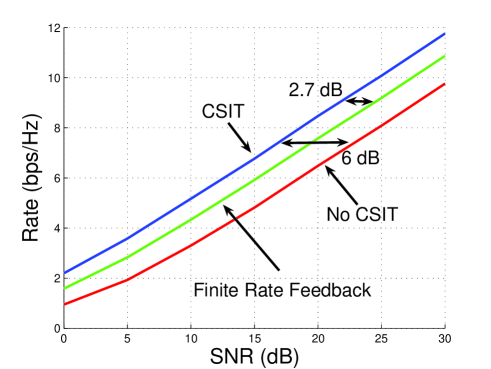
Figure 2: 4 x 1 MISO System with CSIT, No CSIT, & Feedback

The key point to take from this discussion is that the feedback load need not be increased as a function of SNR in order to maintain a constant power or rate gap relative to the perfect CSIT capacity curve. This is perhaps not surprising, since the amount of feedback only affects the $\cos^{2}\left(\angle({\bf h},\hat{\bf h})\right)$ term and thus leads to only a SNR degradation. Furthermore, also note that the multiplexing gain (i.e., the slope of the capacity curve) is not affected by the level of CSIT. For the MIMO downlink channel, however, the multiplexing gain of a $M$-transmit antenna, $K$ user system is $\min(N,K)$ when there is perfect CSIT, but is only $1$ if there is no CSIT. Clearly such a channel will be considerably more sensitive to the accuracy of the CSIT obtained through the finite rate feedback channels.

IV Downlink Precoding with Finite Rate Feedback

After the transmitter has received feedback bits from each of the $K$ receivers, an appropriate multi-user transmission strategy must be chosen. We propose using zero-forcing beamforming based on the channel quantizations available at the transmitter. Zero-forcing (ZF) is a low complexity transmission scheme that can be implemented by a simple linear precoder, and its performance is optimal amongst the set of all linear precoders at asymptotically high SNR [19]. We later provide numerical results describing the performance of regularized zero-forcing precoding [30], which outperforms pure zero-forcing at low SNR’s but is equivalent to ZF at asymptotically high SNR.

Note that dirty paper coding cannot be directly applied in this scenario because of the imperfection in CSIT. In order to implement DPC, the transmitter in fact requires knowledge of the multi-user interference at the receiver, and not at the transmitter. The received interference clearly depends on the channel state, which is not known perfectly at the transmitter in the finite rate feedback model. The transmitter could estimate the received interference based on the available channel quantization, but even this estimated interference cannot be cancelled perfectly using DPC due to the transmitter’s imperfect knowledge of the received signal power. In order to implement DPC, the transmitter must also know the received SNR (in the absence of any interference) in order to properly select the inflation factor, which is a key component in the dirty paper coding implementation [23]. Since the SNR also depends on the channel realization, the transmitter only has an imperfect estimate of the SNR and thus cannot properly select the inflation factor.

When the transmitter has perfect CSI, zero-forcing can be used to completely eliminate multi-user interference by precoding transmission by the inverse of the channel matrix ${\bf H}$. This creates a parallel, non-interfering channel to each of the $M$ receivers, and thus leads to a multiplexing gain of $M$. In the finite rate feedback setting, the imperfection in CSIT makes it impossible to completely eliminate all multi-user interference, but a zero-forcing based strategy can still be quite effective. Since the transmitter only has knowledge of the channel quantizations but does not have any information regarding the magnitude or spatial direction of the quantization error, a reasonable approach to take is to select beamforming vectors according to the zero-forcing criterion based on the channel quantizations.

Let $\hat{\bf h}_{i}$ refer to the quantized version of the mobile $i$’s channel. These quantized vectors are compiled into a matrix: $\hat{\bf H}=\left[\begin{array}[]{cccc}\hat{\bf h}_{1}&\hat{\bf h}_{2}&\cdots&\hat{\bf h}_{M}\end{array}\right]^{\dagger}$. The matrix ${\hat{\bf H}}$ is the estimate of the channels, upon which zero-forcing is performed. Thus, the beamforming vectors are chosen to be the normalized columns of the matrix ${\hat{\bf H}}^{-1}$. If equal power $\frac{P}{M}$ is used for each of the data streams, the received SINR at the $i$-th mobile is given by (7):

$$SINR_{i}=\frac{\frac{P}{M}|{\mathbf{h}}_{i}^{\dagger}{\mathbf{v}}_{i}|^{2}}{1+\sum_{j\neq i}\frac{P}{M}|{\mathbf{h}}_{i}^{\dagger}{\mathbf{v}}_{j}|^{2}}.$$ (10)

Since the beamforming vectors are chosen orthogonal to the channel quantizations and not the actual channel realizations, the interference terms in the denominator of the SINR expression are not zero. However, these terms directly depend on the quantization error and thus can be analyzed using the statistics of random vector quantization.

We study long-term average throughput (over both the fading distribution and RVQ), and thus the rate of transmission to User $i$ is equal to $R_{i}=E_{\mathbf{H},{\mathcal{W}}}\left[\log_{2}(1+SINR_{i})\right]$ if Gaussian inputs are used. By symmetry, the system throughput is given by:

$$R_{FB}(P)\triangleq ME_{\mathbf{H},{\mathcal{W}}}\left[\log_{2}(1+SINR)\right].$$

For a system that achieves a throughput of $R(P)$ (where $P$ is the SNR, or power constraint), the multiplexing gain is defined as:

$$r=\lim_{P\rightarrow\infty}\frac{R(P)}{\log_{2}(P)}.$$ (11)

V Throughput Analysis

In this section we analyze the throughput of a feedback-based zero-forcing system. We first state some useful preliminary calculations, and then study the achieved throughput for fixed and increasing feedback levels.

V-A Preliminary Calculations

In this section we prove a few useful results regarding the distribution of terms in the SINR expression in (10). For the remainder of this paper, we use $\tilde{\bf{h}}_{i}$ to denote the normalized channel vector, i.e., $\tilde{\bf{h}}_{i}={\bf{h}}_{i}/||{\bf{h}}_{i}||$. Using this notation, we can rewrite the SINR as:

$$SINR_{i}=\frac{\frac{P}{M}||{\bf{h}}_{i}||^{2}|\tilde{\mathbf{h}}_{i}^{\dagger}{\mathbf{v}}_{i}|^{2}}{1+\sum_{j\neq i}\frac{P}{M}||{\bf{h}}_{i}||^{2}|\tilde{\mathbf{h}}_{i}^{\dagger}{\mathbf{v}}_{j}|^{2}}.$$ (12)

We first characterize the numerator of this expression, i.e., the received signal power:

Lemma 2

The beamforming vector ${\bf v}_{i}$ is isotropically distributed in $\mathbb{C}^{M}$ and is independent of the channel direction $\tilde{\bf h}_{i}$ as well as the channel quantization $\hat{\bf h}_{i}$.

Proof:

By the zero-forcing procedure, ${\bf v}_{i}$ is chosen in the nullspace of $\{\hat{\bf h}_{j}\}_{j\neq i}$. Since RVQ is used and the channel directions $\{\tilde{\bf h}_{j}\}_{j\neq i}$ are independent isotropic vectors, the channel quantizations $\hat{\bf{h}}_{1},\ldots,\hat{\bf{h}}_{M}$ are mutually independent isotropically distributed vectors. Thus the nullspace of $\{\hat{\bf h}_{j}\}_{j\neq i}$ is an isotropically distributed direction in $\mathbb{C}^{M}$, independent of either $\tilde{\bf h}_{i}$ or $\hat{\bf h}_{i}$. ∎

Clearly the same argument holds if the transmitter performs zero-forcing on the basis of perfect CSIT (i.e., $\hat{\bf h}_{i}=\tilde{\bf h}_{i}$).

Next we characterize the interference terms that appear in the denominator of the SINR expression:

Lemma 3

The random variable $|\tilde{\mathbf{h}}_{i}^{\dagger}{\mathbf{v}}_{j}|^{2}$ for any $i\neq j$ is equal to the product of the quantization error $\sin^{2}\left(\angle(\tilde{\bf h}_{i},\hat{\bf h}_{i})\right)$ and an independent beta $(1,M-2)$ random variable.

Proof:

Without loss of generality, consider $i=2$ and $j=1$, i.e. the term $|\tilde{\mathbf{h}}_{2}^{\dagger}{\mathbf{v}}_{1}|^{2}$. The vector ${\mathbf{v}}_{1}$ is chosen in the nullspace of $\hat{\bf{h}}_{2},\ldots,\hat{\bf{h}}_{M}$, each of which is an independent isotropically distributed vector. Therefore, ${\mathbf{v}}_{1}$ is isotropically distributed within the $(M-1)$-dimensional nullspace of $\hat{\bf{h}}_{2}$. Now consider the normalized channel vector $\tilde{\bf{h}}_{2}$. Since RVQ is used, the quantization error has no preferential direction, i.e. the error is isotropically distributed in $\mathbb{C}^{M}$. Thus, conditioned on the magnitude of the quantization error $a\triangleq\sin^{2}\left(\angle(\tilde{\bf h}_{i},\hat{\bf h}_{i})\right)$, the channel direction can be written as the sum of two vectors, one in the direction of the quantization, and the other isotropically distributed in the nullspace of the quantization: $\tilde{\bf{h}}_{2}=\sqrt{1-a}\hat{\bf{h}}_{2}+\sqrt{a}{\mathbf{s}}$, where ${\mathbf{s}}$ is isotropically distributed in the nullspace of $\hat{\bf{h}}_{2}$, and is independent of $a$. Therefore, the random variable $\tilde{\bf{h}}_{2}$ can be written as:

$$\tilde{\bf{h}}_{2}=(\sqrt{1-Z})\hat{\bf{h}}_{2}+\sqrt{Z}{\mathbf{s}},$$

where ${\bf s}$ and $Z$ are independent, with ${\bf s}$ isotropically distributed in the nullspace of $\hat{\bf{h}}_{2}$ and $Z$ distributed according to the quantization error distribution, i.e., the minimum of $2^{B}$ beta $(M-1,1)$ random variables, as described in Section III-C.

The inner product of $\tilde{\bf{h}}_{2}$ and ${\mathbf{v}}_{1}$ is then given by:

$$|\tilde{\mathbf{h}}_{2}^{\dagger}{\mathbf{v}}_{1}|^{2} = (1-Z)|\hat{\bf{h}}_{2}^{\dagger}{\mathbf{v}}_{1}|^{2}+Z|{\mathbf{s}}^{\dagger}{\mathbf{v}}_{1}|^{2}$$

$$= Z|{\mathbf{s}}^{\dagger}{\mathbf{v}}_{1}|^{2}.$$

Since ${\bf s}$ and ${\bf v}_{1}$ are iid isotropic vectors in the $(M-1)$-dimensional nulllspace of $\hat{\bf{h}}_{2}$, the quantity $|{\mathbf{s}}^{\dagger}{\mathbf{v}}_{1}|^{2}$ is beta $(1,M-2)$ distributed, and is independent of $Z$. ∎

Since a beta random variable has support $[0,1]$, we have

$$|\tilde{\mathbf{h}}_{i}^{\dagger}{\mathbf{v}}_{j}|^{2}\leq\sin^{2}\left(\angle(\tilde{\bf h}_{i},\hat{\bf h}_{i})\right),~{}~{}~{}~{}\forall i\neq j,$$ (13)

i.e., the interference from any single user is no larger than the quantization error. When $M=2$, we clearly have $|\tilde{\mathbf{h}}_{i}^{\dagger}{\mathbf{v}}_{j}|^{2}=\sin^{2}\left(\angle(\tilde{\bf h}_{i},\hat{\bf h}_{i})\right)$, and no beta random variable is needed.

Finally, a derivation of the expectation of the logarithm of the quantization error, which is useful in a few subsequent theorems, is given:

Lemma 4

The expectation of the logarithm of the quantization error is given by:

$$E_{\mathbf{H},{\mathcal{W}}}\left[\log_{2}\left(\sin^{2}(\angle(\tilde{\mathbf{h}}_{i},\hat{{\bf h}}_{i}))\right)\right]=-\frac{\log_{2}e}{M-1}\sum_{k=1}^{2^{B}}\frac{1}{k}.$$

Furthermore, this quantity can be bounded as:

$$\frac{B}{M-1}\leq-E_{\mathbf{H},{\mathcal{W}}}\left[\log_{2}\left(\sin^{2}(\angle(\tilde{\mathbf{h}}_{i},\hat{{\bf h}}_{i}))\right)\right]\leq\frac{B+\log_{2}e}{M-1}.$$

Proof:

See Appendix C. ∎

V-B Fixed Feedback Quality

We now analyze the average throughput achieved by the proposed zero-forcing scheme, and quantify the performance degradation as a function of the feedback rate. In order to study the performance loss, we define the rate gap $\Delta R(P)$ to be the difference between the per mobile throughput achieved by perfect CSIT-ZF and finite-rate feedback based ZF:

$$\Delta R(P) \triangleq \frac{1}{M}[R_{ZF}(P)-R_{FB}(P)].$$

In this expression $R_{ZF}(P)$ refers to the throughput achieved by perfect CSIT-based zero-forcing (i.e., $\hat{\bf h}_{i}=\tilde{\bf h}_{i}$), which is given by:

$$R_{ZF}(P)=ME_{{\bf H}}\log_{2}\left(1+\frac{P}{M}|{\mathbf{h}}_{i}^{\dagger}{\mathbf{v}}_{ZF,i}|^{2}\right),$$

where each beamforming vector ${\mathbf{v}}_{ZF,i}$ is chosen orthogonal to $\{{\bf h}_{j}\}_{j\neq i}$.

Theorem 1

Finite rate feedback with $B$ feedback bits per mobile incurs a throughput loss relative to perfect CSIT zero forcing that can be upper bounded by:

$$\Delta R(P)<\log_{2}\left(1+P\cdot 2^{-\frac{B}{M-1}}\right).$$

Proof:

The rate gap can be upper bounded as:

$$\Delta R(P) = E_{{\bf H}}\left[\log_{2}\left(1+\frac{P}{M}|{\bf h}_{i}^{\dagger}{\bf v}_{ZF,i}|^{2}\right)\right]-E_{{\bf H},W}\left[\log_{2}\left(1+\frac{\frac{P}{M}|{\mathbf{h}}_{i}^{\dagger}{\mathbf{v}}_{i}|^{2}}{1+\sum_{j\neq i}\frac{P}{M}|{\mathbf{h}}_{i}^{\dagger}{\mathbf{v}}_{j}|^{2}}\right)\right]$$

$$= E_{{\bf H}}\left[\log_{2}\left(1+\frac{P}{M}|{\bf h}_{i}^{\dagger}{\bf v}_{ZF,i}|^{2}\right)\right]-E_{{\bf H},W}\left[\log_{2}\left(1+\frac{P}{M}|{\mathbf{h}}_{i}^{\dagger}{\mathbf{v}}_{i}|^{2}+\sum_{j\neq i}\frac{P}{M}|{\mathbf{h}}_{i}^{\dagger}{\mathbf{v}}_{j}|^{2}\right)\right]$$

$$+E_{{\bf H},W}\left[\log_{2}\left(1+\sum_{j\neq i}\frac{P}{M}|{\mathbf{h}}_{i}^{\dagger}{\mathbf{v}}_{j}|^{2}\right)\right]$$

$$\stackrel{{\scriptstyle(a)}}{{\leq}} E_{{\bf H}}\left[\log_{2}\left(1+\frac{P}{M}|{\bf h}_{i}^{\dagger}{\bf v}_{ZF,i}|^{2}\right)\right]-E_{{\bf H},W}\left[\log_{2}\left(1+\frac{P}{M}|{\mathbf{h}}_{i}^{\dagger}{\mathbf{v}}_{i}|^{2}\right)\right]$$

$$+E_{{\bf H},W}\left[\log_{2}\left(1+\sum_{j\neq i}\frac{P}{M}|{\mathbf{h}}_{i}^{\dagger}{\mathbf{v}}_{j}|^{2}\right)\right]$$

$$\stackrel{{\scriptstyle(b)}}{{=}} E_{{\bf H},W}\left[\log_{2}\left(1+\sum_{j\neq i}\frac{P}{M}|{\mathbf{h}}_{i}^{\dagger}{\mathbf{v}}_{j}|^{2}\right)\right],$$

where (a) follows because $\sum_{j\neq i}\frac{P}{M}|{\mathbf{h}}_{i}^{\dagger}{\mathbf{v}}_{j}|^{2}\geq 0$ and $\log(\cdot)$ is a monotonically increasing function. To get (b), note that ${\bf v}_{ZF,i}$ and ${\bf v}_{i}$ are each isotropically distributed unit vectors, independent of ${\bf h}_{i}$, by Lemma 2, which implies $E_{{\bf H}}\left[\log_{2}\left(1+\frac{P}{M}|{\bf h}_{i}^{\dagger}{\bf v}_{ZF,i}|^{2}\right)\right]=E_{{\bf H},W}\left[\log_{2}\left(1+\frac{P}{M}|{\mathbf{h}}_{i}^{\dagger}{\mathbf{v}}_{i}|^{2}\right)\right]$. Applying Jensen’s inequality and exploiting the independence of the channel norm (which satisfies $E[||{\bf{h}}_{i}||^{2}]=M$) and channel direction, we get:

$$\Delta R(P) \leq \log_{2}\left(1+\frac{P}{M}(M-1)E[||{\bf{h}}_{i}||^{2}]E[|\tilde{\bf h}_{i}^{\dagger}{\bf v}_{j}|^{2}]\right)$$

$$= \log_{2}\left(1+P(M-1)E[|\tilde{\bf h}_{i}^{\dagger}{\bf v}_{j}|^{2}]\right).$$

By Lemma 3, the term $E[|\tilde{\bf h}_{i}^{\dagger}{\bf v}_{j}|^{2}]$ is the product of the expectation of the quantization error and the expectation of a beta$(1,M-2)$ random variable, which is equal to $\frac{1}{M-1}$. Using Lemma 1 we have:

$$\Delta R(P) \leq \log_{2}\left(1+P\cdot E[\sin^{2}(\angle(\tilde{\mathbf{h}}_{i},\hat{{\bf h}}_{i}))]\right)$$

$$< \log_{2}\left(1+P\cdot 2^{-\frac{B}{M-1}}\right).$$

∎

The most important feature to notice is that the rate loss is an increasing function of the system SNR ($P$), which can be explained by the linear relationship between $P$ and the multi-user interference power. This intuition motivates the following result, which shows that a finite-rate feedback system with fixed feedback quality is interference-limited at high SNR:

Theorem 2

The throughput achieved by finite-rate feedback-based zero-forcing with a fixed number of feedback bits per mobile $B$ is bounded as the SNR is taken to infinity:

$$R_{FB}(P) \leq M\left(1+\frac{B+\log_{2}e}{M-1}+\log_{2}e+\log_{2}(M-2)\right).$$

Proof:

Consider the following upper bounds to the throughput $R_{FB}(P)$:

$$\frac{1}{M}R_{FB}(P) = E_{\mathbf{H},{\mathcal{W}}}\left[\log_{2}\left(1+\frac{\frac{P}{M}|{\mathbf{h}}_{i}^{\dagger}{\mathbf{v}}_{i}|^{2}}{1+\sum_{j\neq i}\frac{P}{M}|{\mathbf{h}}_{i}^{\dagger}{\mathbf{v}}_{j}|^{2}}\right)\right]$$

$$\leq E_{\mathbf{H},{\mathcal{W}}}\left[\log_{2}\left(1+\frac{||{\mathbf{h}}_{i}||^{2}|\tilde{\mathbf{h}}_{i}^{\dagger}{\mathbf{v}}_{i}|^{2}}{\sum_{j\neq i}||{\mathbf{h}}_{i}||^{2}|\tilde{\mathbf{h}}_{i}^{\dagger}{\mathbf{v}}_{j}|^{2}}\right)\right]$$

$$\stackrel{{\scriptstyle(a)}}{{\leq}} E_{\mathbf{H},{\mathcal{W}}}\left[\log_{2}\left(1+\frac{|\tilde{\mathbf{h}}_{i}^{\dagger}{\mathbf{v}}_{i}|^{2}}{|\tilde{\mathbf{h}}_{i}^{\dagger}{\mathbf{v}}_{j}|^{2}}\right)\right]$$

$$= E_{\mathbf{H},{\mathcal{W}}}\left[\log_{2}\left(|\tilde{\mathbf{h}}_{i}^{\dagger}{\mathbf{v}}_{j}|^{2}+|\tilde{\mathbf{h}}_{i}^{\dagger}{\mathbf{v}}_{i}|^{2}\right)\right]-E_{\mathbf{H},{\mathcal{W}}}\left[\log_{2}\left(|\tilde{\mathbf{h}}_{i}^{\dagger}{\mathbf{v}}_{j}|^{2}\right)\right]$$

$$\stackrel{{\scriptstyle(b)}}{{\leq}} 1-E_{\mathbf{H},{\mathcal{W}}}\left[\log_{2}\left(|\tilde{\mathbf{h}}_{i}^{\dagger}{\mathbf{v}}_{j}|^{2}\right)\right].$$

where in (a) we consider only one of the multi-user interference terms, and (b) uses the fact that $|\tilde{\mathbf{h}}_{i}^{\dagger}{\mathbf{v}}_{j}|\leq 1$ and $|\tilde{\mathbf{h}}_{i}^{\dagger}{\mathbf{v}}_{i}|\leq 1$. Since $|\tilde{\mathbf{h}}_{i}^{\dagger}{\mathbf{v}}_{j}|^{2}$ is the product of the quantization error and a beta random variable (Lemma 3), we have

$$-E_{\mathbf{H},{\mathcal{W}}}\left[\log_{2}\left(|\tilde{\mathbf{h}}_{i}^{\dagger}{\mathbf{v}}_{j}|^{2}\right)\right] = -E_{\mathbf{H},{\mathcal{W}}}\left[\log_{2}\left(\sin^{2}(\angle(\tilde{\mathbf{h}}_{i},\hat{{\bf h}}_{i}))\right)\right]-E_{Y}\left[\log_{2}Y\right]$$

$$= \frac{\log_{2}e}{M-1}\sum_{k=1}^{2^{B}}\frac{1}{k}+\log_{2}e\sum_{k=1}^{M-2}\frac{1}{k}$$

$$\leq \frac{B+\log_{2}e}{M-1}+\log_{2}(M-2)+\log_{2}e,$$

where we have used Lemma 4 as well as the easily verifiable fact that $E[-\log_{2}Y]=(\log_{2}e)\sum_{k=1}^{M-2}\frac{1}{k}\leq\log_{2}(M-2)+\log_{2}e$ when $Y$ is beta $(1,M-2)$. Plugging this expression into the upper bound on $R_{FB}(P)$ gives the result. ∎

Regardless of how many feedback bits ($B$) are used, the system eventually becomes interference limited because interference and signal power both scale linearly with $P$. In Fig. 3 the performance of a 5 antenna, 5 user system with 10, 15, and 20 feedback bits per mobile is shown. When the SNR is small, limited feedback performs nearly as well as zero-forcing. However, as the SNR is increased, the limited feedback system becomes interference limited and the rates converge to an upper limit, as expected. Although the upper bound in Theorem 2 is quite loose in general, it does correctly predict the roughly linear dependence of the limiting throughput and $B$.

Notice that this interference-limited behavior can easily be avoided by reverting to a TDMA strategy, but this only provides a multiplexing gain of one. However, as validated by numerical results in Section VI, TDMA is preferable to feedback-based zero forcing at high SNR’s if $B$ is kept fixed.

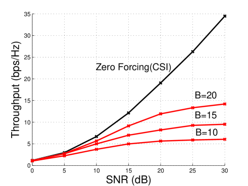
Figure 3: 5 $\times$ 5 Channel with Fixed # Feedback Bits

V-C Increasing Feedback Quality

In the previous section we studied systems with fixed feedback rates, and showed that the throughputs of such systems are bounded. In this section we show that this interference-limited behavior can be avoided by scaling the feedback rate linearly with the SNR (in dB). In fact, if the feedback rate is scaled at the appropriate rate, the full multiplexing gain of $M$ is achievable. In addition to achieving the full multiplexing gain, it is also desirable to maintain a constant rate offset between the rates achievable with zero-forcing with perfect CSI and with finite-rate feedback. Note that if a bounded rate gap is maintained, the full multiplexing gain is also achieved. The following theorem specifies a sufficient scaling of feedback bits to maintain a bounded rate gap:

Theorem 3

In order to maintain a rate offset no larger than $\log_{2}b$ (per user) between zero forcing with perfect CSI and with finite-rate feedback, it is sufficient to scale the number of feedback bits per mobile according to:

$$B = (M-1)\log_{2}P-(M-1)\log_{2}(b-1)$$ (14)

$$\approx \frac{M-1}{3}P_{dB}-(M-1)\log_{2}(b-1).$$ (15)

Proof:

In order to characterize a sufficient scaling of feedback bits, we set the rate gap upper bound given in Theorem 1 equal to the maximum allowable gap of $\log_{2}b$:

$$\Delta R(P)<\log_{2}\left(1+P\cdot 2^{-\frac{B}{M-1}}\right)\triangleq\log_{2}b.$$

By inverting this expression and solving for $B$ as a function of $b$ and $P$ we get:

$$B = (M-1)\log_{2}P-(M-1)\log_{2}(b-1)$$ (16)

$$= \frac{(M-1)\log_{2}10}{10}P_{dB}-(M-1)\log_{2}(b-1)$$ (17)

$$\approx \frac{M-1}{3}P_{dB}-(M-1)\log_{2}(b-1).$$ (18)

With this scaling of feedback bits, we clearly have $\Delta R(P)<\log_{2}b$ for all $P$, as desired. ∎

The rate offset of $\log_{2}b$ (per user) can easily be translated into a power offset, which is a more useful metric from the design perspective. Since a multiplexing gain of $M$ is achieved with zero-forcing, the zero-forcing curve has a slope of $M$ bps/Hz/3 dB at asymptotically high SNR. Therefore, a rate offset of $\log_{2}b$ bps/Hz per user, or equivalently $M\log_{2}b$ bps/Hz in throughput, corresponds to a power offset of $3\log_{2}b$ dB [31][32]. Thus, $b=2$ corresponds to a 3 dB offset, and the resulting scaling of bits takes on a particularly simple form when a 3 dB offset is desired:

$$B=\frac{M-1}{3}P_{dB}~{}~{}\textrm{bits/mobile}$$. (19)

In order to achieve a smaller power offset, $b$ needs to be made appropriately smaller. For example, a 1-dB offset corresponds to $b=10^{1/10}=1.259$ and thus an additional $1.95(M-1)$ feedback bits are required at all SNR’s.

In Fig. 4, throughput curves are shown for a 5 antenna, 5 user system. The feedback load is assumed to scale according to the relationship given in (19), and limited feedback is seen to perform within 2.6 dB of perfect CSI zero-forcing. Notice that the actual power offset is smaller than 3 dB primarily due to the use of Jensen’s inequality in deriving the upper bound to $\Delta R(P)$ in Theorem 1. The sum capacity, which outperforms zero-forcing by 5.55 dB in a $5\times 5$ system [19], is also shown. In Fig. 5, throughput curves are shown for a 6 antenna, 6 user system. In this figure, $B$ is scaled to guarantee a 3 dB and 6 dB gap from perfect CSIT zero-forcing (i.e., $b=2$ and $b=4$ in (15)). Again, the actual gaps are smaller than the bounds (2.5 dB and 5 dB, respectively), but are still sufficiently close to make the bounds useful.

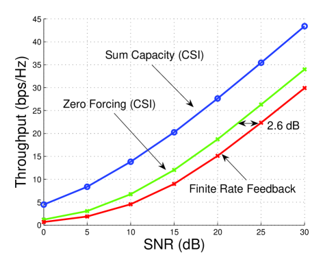
Figure 4: 5 $\times$ 5 Channel with Increasing # Feedback Bits

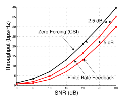
Figure 5: 6 $\times$ 6 Channel with Increasing # Feedback Bits

If $B$ is scaled at a rate strictly greater than $(M-1)\log_{2}P$, i.e. $B=\alpha\log_{2}P$ for any $\alpha>M-1$, the upper bound to the rate gap (Theorem 1) is easily shown to converge to zero:

$$\lim_{P\rightarrow\infty}\Delta R(P)\leq\lim_{P\rightarrow\infty}\log_{2}\left(1+P\cdot 2^{-\frac{B}{M-1}}\right)=0,$$

which implies that the rate gap itself converges to zero. Thus, the throughput achieved with limited feedback converges (absolutely) to the perfect CSIT throughput at asymptotically high SNR.

However, scaling $B$ at a rate slower than $(M-1)\log_{2}P$ results in a strict reduction in the multiplexing gain, as the following theorem shows:

Theorem 4

If $B$ is scaled as $B=\alpha\log_{2}P$ for $\alpha<M-1$, the throughput curve achieves a multiplexing gain of $M\left(\frac{\alpha}{M-1}\right)$.

Proof:

See Appendix D. ∎

Intuitively, the signal power grows linearly with $P$, while the interference power scales as the product of $P$ and the quantization error. Since the quantization error is of order $P^{-\frac{\alpha}{M-1}}$, the interference power scales as $P^{\left(1-\frac{\alpha}{M-1}\right)}$, which gives an SNR that scales as $P^{\frac{\alpha}{M-1}}$. Thus, the resulting multiplexing gain is $M\left(\frac{\alpha}{M-1}\right)$.

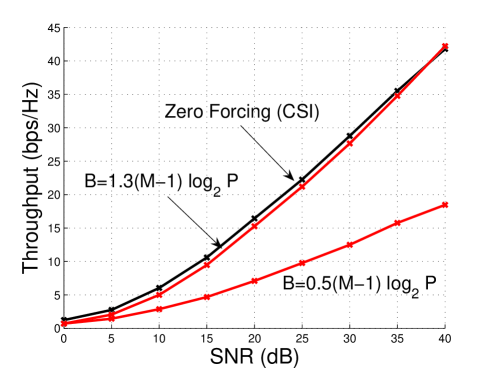
Figure 6: Multiplexing Gain as a Function of Feedback Scaling

In Figure 6 the throughputs achieved with feedback rates given by $B=0.5(M-1)\log_{2}P$ and $B=1.3(M-1)\log_{2}P$ in a $4\times 4$ channel are shown. When $\alpha=0.5(M-1)$, the achieved multiplexing gain is only $0.5M=2$, which corresponds to a slope of 2 bps/Hz per 3 dB. On the other hand, when $\alpha=1.3(M-1)$, the full multiplexing gain is achieved and the rate gap relative to perfect CSIT zero-forcing converges to zero at high SNR.

V-D RVQ vs. Optimal Vector Quantization

Given the previous sections results, an important issue to consider is the possible performance loss incurred by use of random vector quantization instead of an optimal vector quantizer. In this section we derive an upper bound to the bit savings that can result from using optimum vector quantization, and find that the RVQ penalty is actually very small. This is in accordance with results on the optimality of RVQ for point-to-point MIMO and MISO systems [11].

In order to determine the sub-optimality of RVQ, we utilize a lower bound to the quantization error of any vector quantization codebook developed in [33, 5]:

Lemma 5

Consider an arbitrary $B$-bit quantization codebook $\{{\bf w}_{1},\ldots,{\bf w}_{2^{B}}\}$, and let the random variable $Y$ denote the quantization error $Y=\sin^{2}(\angle(\tilde{\bf{h}}_{i},\hat{{\bf{h}}_{i}}))$. The random variable $Y$ stochastically dominates the random variable $\tilde{Z}$, whose CDF is given by:

$$F_{\tilde{Z}}(z)=\left\{\begin{array}[]{ll}2^{B}z^{M-1},&0\leq z\leq 2^{-\frac{B}{M-1}}\\ 1,&z\geq 2^{-\frac{B}{M-1}}\end{array}\right.$$ (22)

or $F_{\tilde{Z}}(z)\geq F_{Y}(z)$ for all $0\leq z\leq 1$.

This lemma applies to the quantization error for a fixed quantization codebook, where the randomness is due only to the isotropic distribution of the channel vector. If RVQ is used, this result can be applied to each quantization codebook, and therefore still holds when considering the random variable describing the quantization error, where there is randomness over both the channel realizations as well as the codebooks:

Corollary 1

If the random variable $Z=\sin^{2}(\angle({\bf{h}}_{i},\hat{{\bf{h}}_{i}}))$ denotes the quantization error achieved when using RVQ (as described in Section III-C), then $Z$ stochastically dominates $\tilde{Z}$, whose CDF is given in (22).

In order to determine the difference between RVQ and and a possibly optimal quantizer, we compute the feedback scaling required to maintain a bounded rate offset as in Theorem 3, but assuming the quantization error is described by $\tilde{Z}$ instead of $Z$. In order to compute this scaling, we first must compute the expectation of $\tilde{Z}$. A simple calculation yields:

$$E[\tilde{Z}] = \int_{0}^{1}\left(1-F_{\tilde{Z}}(z)\right)dz=\left(\frac{M-1}{M}\right)2^{-\frac{B}{M-1}}.$$

Notice that this differs from the upper bound to $E[Z]$ (Lemma 1) only in the term $\frac{M-1}{M}$, and thus the interference power is reduced by at most a factor of $\frac{M-1}{M}$. In order to solve for the required feedback with this bound on the quantization error we set:

$$\log_{2}\left(1+P\cdot\frac{M-1}{M}2^{-\frac{B}{M-1}}\right)\triangleq\log_{2}b,$$

and solve for $B$, which gives:

$$B = (M-1)\log_{2}P-(M-1)\log_{2}(b-1)-(M-1)\log_{2}\left(\frac{M}{M-1}\right).$$ (23)

Comparing this with the similar term for RVQ in (16), we see that the bit savings is a constant factor of $(M-1)\log_{2}\left(\frac{M}{M-1}\right)$ bits at all SNR’s. Furthermore, using the fact that $\log_{e}(1+x)\leq x$ for $x>0$ we have $(M-1)\log_{e}\left(\frac{M}{M-1}\right)=(M-1)\log_{e}\left(1+\frac{1}{M-1}\right)\leq(M-1)\frac{1}{M-1}=1$. Converting to base 2, we see that $(M-1)\log_{2}\left(\frac{M}{M-1}\right)\leq\log_{2}e$ bits, or approximately 1.44 bits. Thus, using RVQ leads to at most a 1.44 bit penalty relative to optimum vector quantization, which is quite small relative to the total feedback load. We should note that this is somewhat of an approximation because we have used Jensen’s inequality to derive the feedback load for both RVQ and for the lower bound. However, numerical results validate the accuracy of Theorem 3, and thus of this metric.

An alternative method to measure RVQ against optimum vector quantization is to compare the performance for the same number of feedback bits, as opposed to the above analysis in which we compared the required feedback load required for identical performance. As stated earlier, the quantization error, and thus the interference, is a factor of $\frac{M-1}{M}$ smaller in the lower bound. If the feedback is scaled in order to maintain a 3 dB gap from perfect CSI zero forcing, the noise and interference term are kept bounded by two (which corresponds to 3 dB). The lower bound, on the other hand, would be $1+\frac{M-1}{M}$ instead of 2. For $M=5$, this corresponds to 2.55 dB, or a 0.45 dB advantage relative to RVQ. As the number of transmit antennas $M$ increases, this gap clearly goes to zero.

V-E Regularized Zero-Forcing

Although zero-forcing precoding performs quite well at moderate and high SNR’s, regularization can significantly increase throughput at low SNR’s [30]. In fact, this is exactly analogous to the difference between zero-forcing equalization and MMSE equalization: while zero-forcing results in complete cancellation of (inter-symbol) interference, an MMSE equalizer alternatively allows a measured amount of interference into the filtered output such that the output SNR is maximized. Regularized zero-forcing is also implemented through a linear precoder, but with a slightly different selection of beamforming vectors. If $\hat{\bf H}$ denotes the concatenation of quantization vectors available to the access point, the zero-forcing beamforming vectors are chosen as the normalized columns of $\hat{\bf H}^{-1}$, or equivalently of $\hat{\bf H}^{\dagger}(\hat{\bf H}\hat{\bf H}^{\dagger})^{-1}$. With regularized zero-forcing, the beamforming vectors ${\bf v}_{1},\ldots,{\bf v}_{K}$ are chosen to be the normalized columns of the matrix:

$$\hat{\bf H}^{\dagger}\left(\hat{\bf H}\hat{\bf H}^{\dagger}+\frac{M}{P}{\bf I}\right)^{-1}.$$

The use of the regularization constant $\frac{M}{P}$ is well motivated by results in [30] as well as the optimal MMSE filters on the dual multiple access channel [16]. It is clear from this regularization that the regularized beamforming vectors will converge to standard zero-forcing vectors at asymptotically high SNR.

Since the rates achieved by zero-forcing and regularized zero-forcing converge at asymptotically high SNR, the feedback scaling specified in Theorem 3 gives the desired rate/power offset for regualarized ZF at asymptotically high SNR. Although we have not been able to extend Theorems 1 or 3 to the rate offset between regularized ZF based on perfect versus feedback-based CSIT, numerical results indicate that these results actually hold at all SNR’s, and not just at very high SNR values. In fact, numerical results indicate that Theorem 3 more accurately predicts the rate offset for regularized ZF than for standard ZF at low and moderate SNR values.

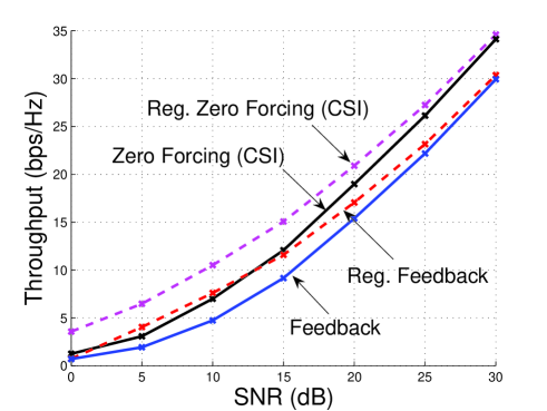
Figure 7: $5\times 5$ Channel with Regularized Zero-Forcing

Throughput curves for zero-forcing (solid lines) and regularized zero-forcing (dotted lines) with perfect CSIT and feedback-based CSIT (with $B=\frac{M-1}{3}P_{dB}$) are shown for a $5\times 5$ channel in Figure 7. The throughput achieved with regularized ZF with perfect CSIT is significantly larger (by approximately 4 bps/Hz) than the throughput with perfect CSIT based ZF for SNR’s between 0 and 15 dB, but the two curves converge at very high SNR. The same is true for the throughput achieved with finite rate feedback and regularized ZF vs. standard ZF. Furthermore, while the rate offset between perfect CSIT-ZF and feedback-CSIT ZF increases from nearly zero at low SNR to its limiting value at high SNR, the rate offset between the two regularized ZF curves is relatively constant over the entire SNR range, as noted earlier.

VI Performance Comparison

In this section we present numerical results comparing the throughput achieved with finite rate feedback and two alternative transmission techniques for the MIMO downlink, random beamforming and TDMA. Because regularized ZF outperforms ZF at all SNR’s, we only consider regularized ZF systems.

Random beamforming is an extension of opportunistic beamforming [34] to the multiple antenna downlink [7]. The transmitter randomly chooses $M$ orthogonal beamforming vectors and transmits pilot symbols along these vectors. Each mobile measures the SINR of each beamforming vector, and feeds back the index of the vector with the highest SINR (requiring $\log_{2}M$ bits), along with the corresponding SINR. The access point then transmits to the best user on each of the beamforming vectors. The required feedback per mobile is quite small ($\log_{2}M$ bits plus an analog SNR value, which will presumably be sufficiently quantized), but this scheme does not perform well in systems with a moderate number of mobiles (i.e., $K\approx M$). In addition, random beamforming is interference limited at asymptotically large SNR if the number of mobiles is kept fixed.

TDMA, in which the access point serves a single user at a time, is perhaps the simplest downlink transmission scheme. We consider the TDMA throughput achievable with perfect CSIT, in which the access point transmits (using the capacity-achieving beamforming strategy) to only the user with the largest SNR. While it is possible to incorporate the effect of finite-rate feedback into a TDMA system (as described in Section III-D), the effect is relatively negligible at the feedback levels considered here and thus for simplicity we consider perfect CSIT. Since a TDMA system achieves a multiplexing gain of only one, we expect to see a significant throughput degradation if TDMA is used, particularly at high SNR. However, note that the difference between the sum capacity of the MIMO downlink (achieved by DPC) and the achievable TDMA throughput is not particularly large at SNR’s less than 5 or 10 dB [2].

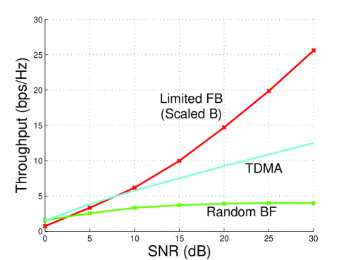
Figure 8: $4\times 4$ Channel with Scaled Feedback, TDMA, & Random BF

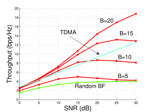
Figure 9: $4\times 4$ Channel with Fixed Feedback, TDMA, & Random BF

Figure 8 plots achievable throughput for a finite-rate feedback system with $B$ scaled to maintain a 3 dB offset (equation (19)), TDMA, and random beamforming, in a $4\times 4$ channel. Finite-rate feedback outperforms random BF beyond 5 dB, which is not surprising given that the feedback level per mobile (which is given by $B=P_{dB}$ for this particular channel) is significantly higher than for random BF. Finite-rate feedback and TDMA give approximately the same throughput up to 10 dB, after which the feedback system begins to significantly outperform TDMA, due to the superior multiplexing gain of the zero-forcing system. The same channel is considered in Figure 9, but with fixed feedback levels ($B=5,10,15,20$) in the finite-rate feedback system. Here we see that TDMA is a better choice than finite-rate feedback with either 5 or 10 bits of feedback per mobile. If 15 or 20 feedback bits are permitted, however, finite-rate feedback can provide a significant advantage over TDMA, particularly above 10 dB.

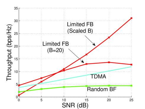
Figure 10: $8\times 8$ Channel with Feedback, TDMA, & Random BF

Figure 10 displays achievable throughput in a $8\times 8$ channel for finite-rate feedback systems with $B$ scaled according to equation (19) and with $B=20$, along with TDMA and random BF throughputs. The throughput achieved with scaled feedback is considerably larger than the TDMA throughput, due to the large number of spatial degrees of freedom used by the zero-forcing system. The 20 feedback bit system outperforms TDMA at moderate SNR’s, but hits the interference limited regime around 15 or 20 dB.

In general, finite-rate feedback based zero-forcing outperforms TDMA at SNR’s above 5 or 10 dB if the feedback per mobile is sufficiently large, but does not provide a significant advantage at low SNR’s. Furthermore, random beamforming is outperformed by both TDMA and finite-rate feedback at essentially all SNR levels. However, this is largely due to the limited number of mobiles, as random beamforming does provide excellent performance in systems with many more mobiles than AP antennas.

VII Conclusions

The use of multi-user MIMO techniques can significantly increase downlink throughput without requiring large numbers of antennas at each mobile device. However, it is crucial that the transmitter have accurate channel state information in order to realize these gains. In fact, the availability of channel state information appears to be the critical issue that will determine the feasibility of multi-user MIMO techniques in future wireless communication systems.

We investigated the finite-rate feedback model, in which each mobile quantizes its channel realization to a finite number of bits that are fed back to the transmitter. Although this model has been extensively studied for point to point MIMO channels, conclusions are quite different in the multi-user setting. Our primary result showed that the number of feedback bits per mobile must be increased linearly with the SNR (in dB) in order to realize multi-user MIMO benefits. As a result of this, feedback levels are quite high in MIMO downlink channels: in a 4 antenna system, for example, each mobile must feed back 10 bits at an overall system SNR of 10 dB. In contrast, feedback does not need to scale with SNR in point to point MIMO systems, and even a relatively small number of bits (e.g., 4 or 5) can be very beneficial at all SNR levels. This scaling relationship is particularly troublesome because multi-user MIMO techniques are generally most beneficial in the high SNR regime.

The intuition for the extreme sensitivity of the MIMO downlink channel to imperfection in CSIT, as compared to point-to-point MIMO channels, is actually quite straightforward. In point-to-point MIMO channels, imperfect CSIT leads to mismatch between the input and the transmission modes of the channel and thus some “wasted” transmission power (e.g., power that is transmitted into the nullspace of the channel), which reduces the received SNR but has no other deleterious effect. In a MIMO downlink channel, imperfect CSIT also leads to mismatch between the input and the channel, but the effect of this is increased multi-user interference, which is significantly more harmful than a reduction in desired signal power.

There are, however, a number of reasons to be optimistic regarding the issue of CSI feedback in downlink channels. First note that we have considered only the most basic iid Rayleigh block fading model, and feedback rates can surely be decreased by exploiting spatial and temporal correlation inherent in any physical fading process, as has already been extensively studied for point to point MIMO channels [35][36][37][38]. Furthermore, recent work has shown that a small number of mobile antennas can be used to significantly improve quantization quality and thereby decrease the required feedback rates [39]. In addition, it may also be possible to exploit multi-user diversity effects and thereby reduce feedback rates in systems with a large number of mobiles [7][13][9]. Within this body of work, one interesting idea is to have only a subset of mobiles (e.g., mobiles meeting a fixed SNR threshold) feed back their channel information [40][41][9]. While this technique can significantly reduce the total number of feedback bits to be transmitted, it also requires contention-based feedback (i.e., random access), which can lead to throughput reduction as well as additional latency on the feedback channels. Although we have considered only digital feedback methods, analog feedback appears to have a number of attractive properties for the downlink channel [42][43][44]. A careful comparison of analog and digital techniques remains to be performed.

We close by mentioning a few important issues not considered in this work. One key assumption made in this work is that the channel feedback is instantaneous. Of course, there will be some non-zero delay associated with transmitting feed back bits from the mobiles to the access point, and this delay can be quite significant in fast fading (large Doppler spread) channels. In fact, numerical results in [44] indicate that feedback delay can severely limit the performance of certain downlink transmission schemes at even moderate levels of Doppler. In addition, each mobile is assumed to have perfect CSI, while there will be non-zero receiver estimation error in any practical system. This will clearly lead to additional imperfection in the CSI provided to the access point, and could have significant effects. Frequency-selective channels also require attention; consider related work on frequency-selective point-to-point MIMO channels [45][46]. Finally, note that we have only considered frequency division duplexed systems. Channel reciprocity can be exploited to acquire downlink channel state information from the uplink in time division duplexed (TDD) channels, although recent results indicate that, somewhat counter-intuitively, TDD may in fact be less attractive than FDD from a channel state information perspective [42]. Many of the tools used here appear to be well suited to analyze the effect of imperfect CSIT in TDD systems as well.

Appendix A Expected Quantization Error

In this appendix we provide an alternative proof for the closed-form representation of the expected quantization error. The following integral representation for the beta function is given in [47, pg. 5]:

$$\beta\left(c,\frac{a}{b}\right)=b\int_{0}^{1}z^{a-1}\left(1-z^{b}\right)^{c-1}dz,~{}~{}a>0,~{}b>0,~{}c>0.$$

With $a=1$, $b=M-1$, and $c=2^{B}+1$ this yields:

$$\beta\left(2^{B}+1,\frac{1}{M-1}\right)=(M-1)\int_{0}^{1}\left(1-z^{M-1}\right)^{2^{B}}dz.$$

Using the fact that $\textrm{Pr}\left(\sin^{2}\left(\angle(\tilde{\bf h}_{i},\hat{\bf h}_{i})\right)\geq z\right)=(1-z^{M-1})^{2^{B}}$, we have:

$$E_{{\bf H},{\mathcal{W}}}\left[\sin^{2}\left(\angle(\tilde{\bf h}_{i},\hat{\bf h}_{i})\right)\right] = \int_{0}^{1}(1-z^{M-1})^{2^{B}}dz$$

$$= \frac{1}{M-1}\beta\left(2^{B}+1,\frac{1}{M-1}\right)$$

$$= \frac{\frac{1}{M-1}\Gamma\left(2^{B}+1\right)\Gamma\left(\frac{1}{M-1}\right)}{\Gamma\left(2^{B}+1+\frac{1}{M-1}\right)}$$

$$= \frac{2^{B}\Gamma\left(2^{B}\right)\Gamma\left(1+\frac{1}{M-1}\right)}{\Gamma\left(2^{B}+1+\frac{1}{M-1}\right)}$$

$$= 2^{B}\cdot\beta\left(2^{B},\frac{M}{M-1}\right),$$

where we have used the fundamental equality $\Gamma(z+1)=z\Gamma(z)$.

Appendix B Proof of Lemma 1

The expected quantization error is given by [26]:

$$E_{{\bf H},{\mathcal{W}}}\left[\sin^{2}\left(\angle(\tilde{\bf h}_{i},\hat{\bf h}_{i})\right)\right]=2^{B}\cdot\beta\left(2^{B},\frac{M}{M-1}\right).$$ (24)

For $M=2$, we have

$$2^{B}\cdot\beta\left(2^{B},2\right) = \frac{2^{B}\Gamma(2^{B})\Gamma(2)}{\Gamma\left(2^{B}+2\right)}$$

$$= \frac{2^{B}\Gamma(2^{B})}{\Gamma\left(2^{B}+2\right)}$$

$$= \frac{\left(2^{B}\right)!}{\left(2^{B}+1\right)!}$$

$$= \left(2^{B}+1\right)^{-1}$$

$$< 2^{-B}.$$

For $M>2$:

$$2^{B}\cdot\beta\left(2^{B},\frac{M}{M-1}\right) = 2^{B}\frac{\Gamma(2^{B})\Gamma\left(1+\frac{1}{M-1}\right)}{\Gamma\left(2^{B}+1+\frac{1}{M-1}\right)}$$

$$\leq \frac{2^{B}\Gamma(2^{B})}{\Gamma\left(2^{B}+1+\frac{1}{M-1}\right)}$$

$$= \frac{\Gamma(2^{B}+1)}{\Gamma\left(2^{B}+1+\frac{1}{M-1}\right)}.$$

The above inequality is reached because $\Gamma(x)\leq 1$ for $1\leq x\leq 2$, due to the convexity of the gamma function [27] and the fact that $\Gamma(1)=\Gamma(2)=1$. By applying Kershaw’s inequality for the gamma function[48]:

$$\frac{\Gamma(x+s)}{\Gamma(x+1)}<\left(x+\frac{s}{2}\right)^{s-1}~{}~{}~{}\forall x>0,~{}0<s<1,$$

with $x=2^{B}+\frac{1}{M-1}$ and $s=1-\frac{1}{M-1}$ we get

$$\frac{\Gamma(2^{B}+1)}{\Gamma\left(2^{B}+1+\frac{1}{M-1}\right)} < \left(2^{B}+\frac{M}{2(M-1)}\right)^{-\frac{1}{M-1}}.$$

Furthermore, the decreasing nature of the function $(\cdot)^{-\frac{1}{M-1}}$ gives a further upper bound of $2^{-\frac{B}{M-1}}$.

Appendix C Proof of Lemma 4

Let $Z=\sin^{2}(\angle(\tilde{\bf h}_{i},\hat{\bf h}_{i}))$ represent the quantization error. As stated in Section III-C, $Z$ is the minimum of $2^{B}$ beta $(M-1,1)$ random variables with CCDF given by: $\textrm{Pr}(Z\geq z)=(1-z^{M-1})^{L}$, where $L=2^{B}$. We wish to compute $E[\log_{e}Z]$, or equivalently $E[-\log_{e}Z]$. Since $0\leq Z\leq 1$, the random variable $-\log_{e}Z$ is non-negative with support $[0,\infty)$. Using the fact that $E[X]=\int_{0}^{\infty}\textrm{Pr}(X\geq x)dx$ for non-negative random variables and the binomial expansion, we have:

$$E[-\log_{e}Z] = \int_{0}^{\infty}\textrm{Pr}(-\log_{e}Z\geq z)dz$$

$$= \int_{0}^{\infty}\textrm{Pr}(Z\leq e^{-z})dz$$

$$= \int_{0}^{\infty}1-(1-e^{-z(M-1)})^{L}dz$$

$$= \int_{0}^{\infty}1-\sum_{k=0}^{L}{L\choose k}(-1)^{k}e^{-z(M-1)k}dz$$

$$= \int_{0}^{\infty}\sum_{k=1}^{L}{L\choose k}(-1)^{k+1}e^{-z(M-1)k}dz$$

$$= \sum_{k=1}^{L}{L\choose k}(-1)^{k+1}\left(\int_{0}^{\infty}e^{-z(M-1)k}dz\right)$$

$$= \frac{1}{M-1}\sum_{k=1}^{L}{L\choose k}\frac{(-1)^{k+1}}{k}$$

$$= \frac{1}{M-1}\sum_{k=1}^{L}\frac{1}{k},$$

where the final line follows from [49, Section 0.155].

Furthermore, since $\log_{e}a=\int_{1}^{a}\frac{1}{x}dx$, we have $\log_{e}L\leq\sum_{k=1}^{L}\frac{1}{k}\leq\log_{e}L+1$. We multiply by $\log_{2}e$ to translate to base 2, and thus get $E[-\log_{2}Z]=\frac{\log_{2}e}{M-1}\sum_{k=1}^{L}\frac{1}{k}$. Using $L=2^{B}$ we get the subsequent bounds.

Appendix D Proof of Theorem 4

The multiplexing gain can be expanded as:

$$m \triangleq \lim_{P\rightarrow\infty}\frac{ME_{{\bf H},W}[R_{FB}(P)]}{\log_{2}P}$$ (25)

$$= \lim_{P\rightarrow\infty}\frac{ME_{{\bf H},W}\left[\log_{2}\left(1+\frac{P}{M}|{\mathbf{h}}_{i}^{\dagger}{\mathbf{v}}_{i}|^{2}+\frac{P}{M}\sum_{j\neq i}|{\mathbf{h}}_{i}^{\dagger}{\mathbf{v}}_{j}|^{2}\right)\right]}{\log_{2}P}$$

$$-\lim_{P\rightarrow\infty}\frac{ME_{{\bf H},W}\left[\log_{2}\left(1+\frac{P}{M}\sum_{j\neq i}|{\mathbf{h}}_{i}^{\dagger}{\mathbf{v}}_{j}|^{2}\right)\right]}{\log_{2}P}$$

$$= M-\lim_{P\rightarrow\infty}\frac{ME_{{\bf H},W}\left[\log_{2}\left(1+\frac{P}{M}\sum_{j\neq i}|{\mathbf{h}}_{i}^{\dagger}{\mathbf{v}}_{j}|^{2}\right)\right]}{\log_{2}P}.$$

The final step follows because

$$\log_{2}\left(1+\frac{P}{M}|{\mathbf{h}}_{i}^{\dagger}{\mathbf{v}}_{i}|^{2}\right)\leq\log_{2}\left(1+\frac{P}{M}|{\mathbf{h}}_{i}^{\dagger}{\mathbf{v}}_{i}|^{2}+\frac{P}{M}\sum_{j\neq i}|{\mathbf{h}}_{i}^{\dagger}{\mathbf{v}}_{j}|^{2}\right)\leq\log_{2}\left(1+P||{\mathbf{h}}_{i}||^{2}\right),$$

and the multiplexing gain of the upper and lower bounds are easily shown to be one.

We first show that $m\leq\frac{\alpha}{M-1}$ (using $L=2^{B}=P^{\alpha}$):

$$E_{{\bf H},W}\left[\log_{2}\left(1+\frac{P}{M}\sum_{j\neq i}|{\mathbf{h}}_{i}^{\dagger}{\mathbf{v}}_{j}|^{2}\right)\right] \geq E_{{\bf H},W}\left[\log_{2}\left(\frac{P}{M}|{\mathbf{h}}_{i}^{\dagger}{\mathbf{v}}_{j}|^{2}\right)\right]$$

$$= \log_{2}\left(\frac{P}{M}\right)+E_{\bf H}\left[\log_{2}||{\bf{h}}_{i}||^{2}\right]+E_{{\bf H},W}\left[\log_{2}|\tilde{\mathbf{h}}_{i}^{\dagger}{\mathbf{v}}_{j}|^{2}\right]$$

$$= \log_{2}P+E_{\mathbf{H},{\mathcal{W}}}\left[\log_{2}\left(\sin^{2}(\angle(\tilde{\mathbf{h}}_{i},\hat{{\bf h}}_{i}))\right)\right]+O(1)$$

$$= -\log_{2}P-\frac{\log_{2}e}{M-1}\sum_{k=1}^{L}\frac{1}{k}+O(1)$$

$$\geq \log_{2}P-\frac{1}{M-1}\log_{2}L+O(1)$$

$$= \left(1-\frac{\alpha}{M-1}\right)\log_{2}P+O(1)$$

where we have used Lemma 4 to evaluate the expectation of the logarithm of the interference term. Plugging this bound in to (25) gives $m\leq M\left(\frac{\alpha}{M-1}\right)$.

To show $m\geq M\left(\frac{\alpha}{M-1}\right)$, we upper bound the limit in (25) using the fact that $|\tilde{\mathbf{h}}_{i}^{\dagger}{\mathbf{v}}_{j}|^{2}\leq\sin^{2}(\tilde{\bf{h}}_{i},\hat{\bf{h}}_{i})$ for any $i\neq j$ (from (13)) and Jensen’s inequality:

$$E_{{\bf H},W}\left[\log_{2}\left(1+\frac{P}{M}\sum_{j\neq i}||{\bf{h}}_{i}||^{2}|\tilde{\mathbf{h}}_{i}^{\dagger}{\mathbf{v}}_{j}|^{2}\right)\right] \leq E_{{\bf H},W}\left[\log_{2}\left(1+\frac{P}{M}(M-1)||{\bf{h}}_{i}||^{2}\sin^{2}(\tilde{\bf{h}}_{i},\hat{\bf{h}}_{i})\right)\right]$$

$$\leq \log_{2}\left(1+P(M-1)E\left[\sin^{2}(\tilde{\bf{h}}_{i},\hat{\bf{h}}_{i})\right]\right)$$

$$\leq \log_{2}\left(1+P(M-1)2^{-\frac{B}{M-1}}\right)$$

$$= \log_{2}\left(1+(M-1)P^{\left(1-\frac{\alpha}{M-1}\right)}\right)$$

Thus we have

$$\lim_{P\rightarrow\infty}\frac{ME_{{\bf H},W}\left[\log_{2}\left(1+\frac{P}{M}\sum_{j\neq i}|{\mathbf{h}}_{i}^{\dagger}{\mathbf{v}}_{j}|^{2}\right)\right]}{\log_{2}P}\leq M\left(1-\frac{\alpha}{M-1}\right),$$

which gives $m\geq M\left(\frac{\alpha}{M-1}\right)$.

References

- [1] G. Caire and S. Shamai, “On the achievable throughput of a multiantenna Gaussian broadcast channel,” IEEE Trans. Inform. Theory, vol. 49, no. 7, pp. 1691–1706, July 2003.
- [2] N. Jindal and A. Goldsmith, “Dirty paper coding vs. TDMA for MIMO broadcast channels,” IEEE Trans. Inform. Theory, vol. 51, no. 5, pp. 1783–1794, May 2005.
- [3] A. Narula, M. J. Lopez, M. D. Trott, and G. W. Wornell, “Efficient use of side information in multiple antenna data transmission over fading channels,” IEEE J. Select. Areas Commun., vol. 16, no. 8, Oct. 1998.
- [4] D. Love, R. Heath, and T. Strohmer, “Grassmannian beamforming for multiple-input multiple-output wireless systems,” IEEE Trans. Inform. Theory, vol. 49, no. 10, pp. 2735–2747, Oct. 2003.
- [5] K. Mukkavilli, A. Sabharwal, E. Erkip, and B. Aazhang, “On beamforming with finite rate feedback in multiple-antenna systems,” IEEE Trans. Inform. Theory, vol. 49, no. 10, pp. 2562–2579, Oct. 2003.
- [6] D. Love, R. Heath, W. Santipach, and M. Honig, “What is the value of limited feedback for MIMO channels?” IEEE Communications Magazine, vol. 42, no. 10, pp. 54–59, Oct. 2004.
- [7] M. Sharif and B. Hassibi, “On the capacity of MIMO broadcast channels with partial side information,” IEEE Trans. Inform. Theory, vol. 51, no. 2, pp. 506–522, Feb. 2005.
- [8] T. Yoo and A. Goldsmith, “On the optimality of multiantenna broadcast scheduling using zero-forcing beamforming,” IEEE J. Select. Areas in Commun., vol. 24, no. 3, pp. 528–541, March 2006.
- [9] C. Swannack, E. Uysal-Biyikoglu, and G. Wornell, “MIMO broadcast scheduling with limited channel state information,” in Proceedings of Allerton Conf. on Commun., Control, and Comput., Oct 2005.
- [10] W. Santipach and M. Honig, “Signature optimization for CDMA with limited feedback,” IEEE Trans. Inform. Theory, vol. 51, no. 10, pp. 3475–3492, Oct. 2005.
- [11] ——, “Asymptotic capacity of beamforming with limited feedback,” in Proceedings of Int. Symp. Inform. Theory, July 2004, p. 290.
- [12] P. Ding, D. Love, and M. Zoltowski, “Multiple antenna broadcast channels with shape feedback and limited feedback,” 2005, submitted to IEEE Trans. Sig. Proc.
- [13] T. Yoo, N. Jindal, and A. Goldsmith, “Finite rate feedback MIMO broadcast channels with a large number of users,” submitted to ISIT 2006.
- [14] H. Weingarten, Y. Steinberg, and S. Shamai, “The capacity region of the Gaussian MIMO broadcast channel,” in Proceedings of Conference on Information Sciences and Systems, March 2004.
- [15] S. Vishwanath, N. Jindal, and A. Goldsmith, “Duality, achievable rates, and sum-rate capacity of MIMO broadcast channels,” IEEE Trans. Inform. Theory, vol. 49, no. 10, pp. 2658–2668, Oct. 2003.
- [16] P. Viswanath and D. N. Tse, “Sum capacity of the vector Gaussian broadcast channel and uplink-downlink duality,” IEEE Trans. Inform. Theory, vol. 49, no. 8, pp. 1912–1921, Aug. 2003.
- [17] W. Yu and J. M. Cioffi, “Sum capacity of Gaussian vector broadcast channels,” IEEE Trans. Inform. Theory, vol. 50, no. 9, pp. 1875–1892, Sept. 2004.
- [18] M. Costa, “Writing on dirty paper,” IEEE Trans. Inform. Theory, vol. 29, no. 3, pp. 439–441, May 1983.
- [19] N. Jindal, “A high SNR analysis of MIMO broadcast channels,” in Proceedings of IEEE Int. Symp. Inform. Theory, Sept 2005.
- [20] T. Cover, “Broadcast channels,” IEEE Trans. Inform. Theory, vol. 18, no. 1, pp. 2–14, Jan. 1972.
- [21] S. Jafar and A. Goldsmith, “Isotropic fading vector broadcast channels: The scalar upperbound and loss in degrees of freedom,” IEEE Trans. Inform. Theory, vol. 51, no. 3, pp. 848–857, March 2005.
- [22] A. Lapidoth, S. Shamai, and M. Wigger, “On the capacity of a MIMO fading broadcast channel with imperfect transmitter side-information,” in Proceedings of Allerton Conf. on Commun., Control, and Comput., Sept. 2005.
- [23] R. Zamir, S. Shamai, and U. Erez, “Nested linear/lattice codes for structured multiterminal binning,” IEEE Trans. on Inform. Theory, vol. 48, no. 6, pp. 1250–1276, 2002.
- [24] S. ten Brink and U. Erez, “A close-to-capacity dirty paper coding scheme,” in Proceedings. Int. Symp. Inform. Theory, 2004.
- [25] T. Philosof, U. Erez, and R. Zamir, “Combined shaping and precoding for interference cancellation at low SNR,” in Proceedings. Int. Symp. Inform. Theory, 2003.
- [26] C. Au-Yeung and D. J. Love, “On the performance of random vector quantization limited feedback beamforming in a MISO system,” to appear, IEEE Trans. Wireless Commun.
- [27] J. P. Davis, “Leonhard Euler’s integral: A historical profile of the gamma function,” American Mathematics Monthly, vol. 66, no. 10, pp. 849–869, Dec. 1959.
- [28] E. Telatar, “Capacity of multi-antenna Gaussian channels,” European Trans. on Telecomm. ETT, vol. 10, no. 6, pp. 585–596, November 1999.
- [29] S. A. Jafar and S. Srinivasa, “On the optimality of beamforming with quantized feedback,” submitted to IEEE Trans. Inform. Theory.
- [30] C. Peel, B. Hochwald, and A. Swindlehurst, “Vector-perturbation technique for near-capacity multiantenna multiuser communication-Part I: channel inversion and regularization,” IEEE Trans. on Communications, vol. 53, no. 1, pp. 195–202, 2005.
- [31] S. Shamai and S. Verdu, “The impact of frequency-flat fading on the spectral efficiency of CDMA,” IEEE Trans. Inform. Theory, vol. 47, no. 4, pp. 1302–1327, May 2001.
- [32] A. Lozano, A. Tulino, and S. Verdu, “High-snr power offset in multiantenna communication,” IEEE Trans. Inform. Theory, vol. 51, no. 2, pp. 4134–4151, Dec. 2005.
- [33] S. Zhou, Z. Wang, and G. Giannakis, “Quantifying the power loss when transmit beamforming relies on finite rate feedback,” IEEE Trans. on Wireless Commun., vol. 4, no. 4, pp. 1948–1957, 2005.
- [34] P. Viswanath, D. Tse, and R. Laroia, “Opportunistic beamforming using dumb antennas,” IEEE Trans. Inform. Theory, vol. 48, no. 6, pp. 1277–1294, June 2002.
- [35] D. Love and R. Heath, “Grassmannian beamforming on correlated MIMO channels,” in Proceedings of IEEE Globecom, vol. 1, 2004, pp. 106–110.
- [36] P. Xia and G. B. Giannakis, “Design and analysis of transmit-beamforming based on limited-rate feedback,” in Proceedings of IEEE Vehicular Tech. Conf., 2004.
- [37] V. Raghavan, A. Sayeed, and N. Boston, “Near-optimal codebook constructions for limited-feedback beamforming in correlated MIMO channels,” submitted to ISIT 2006.
- [38] B. Banister and J. Zeidler, “Feedback assisted stochastic gradient adaptation of multiantenna transmission,” IEEE Trans. Wireless Commun., vol. 4, no. 3, pp. 1121–1135, May 2005.
- [39] N. Jindal, “A feedback reduction technique for MIMO broadcast channels,” submitted to ISIT 2006.
- [40] D. Gesbert and M. S. Alouini, “Selective multi-user diversity,” in Proceedings of Int. Symp. on Signal Proc. and Inform. Technology, Dec. 2003.
- [41] S. Sanayei and A. Nosratinia, “Opportunistic downlink transmission with limited feedback,” submitted to IEEE Trans. Inform. Theory, Aug. 2005.
- [42] T. Marzetta and B. Hochwald, “Fast transfer of channel state information in wireless channels,” submitted to IEEE Trans. Sig. Proc. Preprint available at http://mars.bell-labs.com.
- [43] T. Thomas, K. Baum, and P. Sartori, “Obtaining channel knowledge for closed-loop multi-stream broadband MIMO-OFDM communications using direct channel feedback,” in Proceedings of IEEE Globecom, 2005.
- [44] G. Caire, “MIMO downlink joint processing and scheduling: a survey of classical and recent results,” in Proceedings of Workshop on Information Theory and its Applications, San Diego, CA, 2006.
- [45] J. Choi and R. W. Heath, “Interpolation based transmit beamforming for MIMO-OFDM with limited feedback,” IEEE Trans. on Signal Processing, vol. 53, no. 11, pp. 4125–4135, Nov. 2005.
- [46] N. Khaled, B. Mondal, R. W. Heath, G. Leus, and F. Petre, “Interpolation- based multi-mode precoding for MIMO-OFDM systems with limited feedback,” submitted to IEEE Trans. Wireless Commun.
- [47] A. Gupta and S. Nadarajah, Handbook of Beta Distribution and Its Application. Marcel Dekker, Inc., 2004.
- [48] D. Kershaw, “Some extensions of W. Gautschi’s inequalities for the gamma function,” Mathematics of Computation, vol. 41, no. 164, pp. 607–611, Oct. 1983.
- [49] I. S. Gradshteyn, I. M. Ryzhik, A. Jeffrey, and D. Zwillinger, Table of Integrals, Series, and Products, 6th Edition. Academic Press, 2000.