On the Information Rate of MIMO Systems with Finite Rate Channel State Feedback Using Beamforming and Power On/Off Strategy

Abstract

It is well known that Multiple-Input Multiple-Output (MIMO) systems have high spectral efficiency, especially when channel state information at the transmitter (CSIT) is available. When CSIT is obtained by feedback, it is practical to assume that the channel state feedback rate is finite and the CSIT is not perfect. For such a system, we consider beamforming and power on/off strategy for its simplicity and near optimality, where power on/off means that a beamforming vector (beam) is either turned on with a constant power or turned off. The main contribution of this paper is to accurately evaluate the information rate as a function of the channel state feedback rate. Name a beam turned on as an on-beam and the minimum number of the transmit and receive antennas as the dimension of a MIMO system. We prove that the ratio of the optimal number of on-beams and the system dimension converges to a constant for a given signal-to-noise ratio (SNR) when the numbers of transmit and receive antennas approach infinity simultaneously and when beamforming is perfect. Asymptotic formulas are derived to evaluate this ratio and the corresponding information rate per dimension. The asymptotic results can be accurately applied to finite dimensional systems and suggest a power on/off strategy with a constant number of on-beams. For this suboptimal strategy, we take a novel approach to introduce power efficiency factor, which is a function of the feedback rate, to quantify the effect of imperfect beamforming. By combining power efficiency factor and the asymptotic formulas for perfect beamforming case, the information rate of the power on/off strategy with a constant number of on-beams is accurately characterized.

I Introduction

This paper considers multiple-input multiple-output (MIMO) systems with finite rate channel state feedback. Multiple-antenna wireless communication systems, also known as MIMO systems, have high spectral efficiency. It is also well known that the capacity of MIMO systems with channel state information (CSI) at the transmitter (CSIT) is generally higher than the systems without it. When perfect CSI is available at both transmitter and receiver (CSITR), the MIMO channel can be viewed as a set of parallel sub-channels. The transmission power on each sub-channel obeys water filling principle [1]. If CSIT is obtained from channel state feedback, however, perfect CSIT requires infinite feedback rates, which is not practical. On the other hand, in practical systems such as UMTS-HSDPA [2], there is a control field which can be used to carry a certain number of channel state feedback bits on a per-fading block basis. It is reasonable to consider MIMO systems with finite rate channel state feedback.

For a given feedback rate, this paper tries to answer two basic questions, how much benefit the feedback can bring and how to exploit the feedback to achieve that benefit. It is difficult to answer these two questions in general. To achieve or calculate the information rate for a given feedback rate, the optimal transmission strategy and the optimal feedback strategy need to be found. It has been shown in [3, 4] that the design of transmission and feedback strategies is an unconventional optimization problem. For memoryless channels, it is proved that the information theoretic limit can be achieved by memoryless transmission and feedback strategies. However, the explicit forms of the optimal strategies are still unknown. Lloyd algorithm is resorted to obtain suboptimal numerical solution in [3, 4].

On the other hand, the optimization problems can be simplified if the transmission strategy is restricted to power on/off strategy (with beamforming). In a general setting, the optimal transmission strategy is to choose the covariance matrix of the transmitted Gaussian coded symbols according to the current feedback [3, 4]. By the singular value decomposition, the covariance matrix can be decomposed to a unitary matrix and a non-negative diagonal matrix which are called as beamforming matrix and power control matrix respectively. We describe each column vector of the beamforming matrix as a beam and the diagonal element corresponding to a beam as the power on that beam. The power on/off strategy means that a beam is either turned on, i.e., its power is a positive constant $P_{\mathrm{on}}$, or turned off, i.e., its power is zero. As we will show later, the power on/off and beamforming assumption simplifies the analysis. Although power on/off is suboptimal, it has been shown in [5] and [6] that power on/off can achieve performance close to water filling power control for single antenna systems and parallel Gaussian channels respectively. This paper will show that power on/off is near optimal for MIMO channels as well.

The main contribution of this paper is to accurately characterize the information rate of the power on/off strategy with finite rate channel state feedback. Name a beam turned on as an on-beam. The optimization problem corresponding to power on/off strategy is to find the optimal number of on-beams, which is related to power control, and the directions of the on-beams, which is called as beamforming, according to the channel realization. Both power control and beamforming have influence on the overall information rate. By analyzing these two effects separately, this paper is able to characterize the overall information rate accurately.

To isolate the effect of beamforming, we first discuss the perfect beamforming case. Perfect beamforming means that the beamforming matrix at the transmitter changes the MIMO channel to parallel channels without interference. We analyze this case by asymptotics, where the numbers of the transmit and receive antennas approach infinity simultaneously. The derived asymptotic results are as follows.

• Define the minimum number of transmit and receive antennas as the dimension of a MIMO system. We prove that the ratio of the optimal number of on-beams and the system dimension converges to a constant for a given signal-to-noise ratio (SNR) and perfect beamforming. This result suggest a power on/off strategy with a constant number of on-beams. The assumption of a constant number of on-beams is crucial to analyze the effect of imperfect beamforming.

• We also prove that the optimal number of on-beams is a non-decreasing function of SNR.

• We derive asymptotic formulas to simplify the calculations. By following the method developed in [7, 8], we derive asymptotic formulas to evaluate the optimal number of on-beams and the corresponding information rate, which are obtained by simulation traditionally. Furthermore, for the CSITR case, asymptotic formulas are derived to calculate the Lagrange multiplier required for water filling power control and the corresponding channel capacity for the first time.

It is noteworthy that the asymptotic results are accurate enough for MIMO systems with finite many antennas.

Then we quantify the effect of imperfect beamforming accurately by assuming a constant number of on-beams. There are many works studying similar problems. Some works add some structures to make the MIMO system equivalent to a single-input single-output (SISO) system. The structures could be single receive antenna [9, 10, 11, 12, 13] and single beam for a single data stream [14, 15, 16, 17]. For MIMO systems with multiple beams, transmit antenna subset selection is viewed as a special case. Different antenna selection criteria are proposed in [18, 19] and the effect on information rate is analyzed for extreme SNR regimes in [20, 21], whose analysis is hard to be generalized to other SNR regimes. For general multiple beams, assuming that the transmitter knows some singular vectors of the channel matrix perfectly, power allocation to maximize information rate is discussed in [22] and beamforming matrix selection to minimize Bit Error Rate (BER) is proposed in [23]. More practically, if the information about the channel state is obtained through a finite rate feedback, it is reasonable to assume that the transmitter only knows quantized information about the channel state. The popular strategy is to construct a finite size beamforming codebook and select a beamforming matrix for transmission according to the channel state feedback. The algorithms to construct a beamforming codebook are proposed in [24, 25, 26]. The beamforming codebook design criteria and the beamforming matrix feedback criteria, which are often coupled, are discussed in [27, 28, 29, 23, 30]. Based on Grassmann manifolds, the effect of finite beamforming on performance is analyzed in [29, 27] and refined later in [31], all of which are based on Barg’s formula [32] which is only valid for MIMO systems with asymptotically large number of transmit antennas but fixed finite receive antennas. Applied for all MIMO systems, the performance of finite beamforming is analyzed for high SNR region in [30], which is difficult to be generalized to other SNR regimes. Valid for all SNR regimes, the information rate is quantified in [33, 34] by letting the numbers of transmit and receive antennas approach infinity simultaneously and applying extreme order statistics. The proposed formula over-estimates the performance. A correction of the result is in [35]. In the presenting paper, we take a novel approach by introducing the power efficiency factor to quantify the effect of imperfect beamforming. The power efficiency factor can be calculated using a closed form formula derived in [36], which is valid for MIMO systems with arbitrary number of antennas. As a result, the information rate is accurately analyzed as a function of feedback rate. The analysis matches the simulations almost perfectly for all SNR regimes.

Finally, we show the near optimality of the power on/off strategy with a constant number of on-beams by comparing it with a general power on/off strategy. For a general power on/off strategy, we derive the optimal feedback strategy for a given arbitrary beamforming codebook. Then we are able to compare the two different power on/off strategies numerically. Simulations show that a constant number of on-beams is near optimal for all SNR regimes. Therefore, power on/off strategy with a constant number of on-beams provides a simple but near optimal solution.

This paper is organized as follows. The system model and the related design problem are outlined in Section II, where preliminary knowledge about random matrices and Stiefel and Grassmann manifolds are also presented. In Section III, the power on/off strategy with a constant number of on-beams is derived as the optimal solution for perfect beamforming. Section IV considers the effect of imperfect beamforming due to finite rate channel state feedback. Section V shows that a constant number of on-beams is also near optimal for imperfect beamforming. Conclusions are given in Section VI.

II Preliminaries

In this section, we first describe the system model. Then we present some preliminary knowledge about random matrices and Stiefel and Grassmann manifolds.

In this paper, we use $\mathbb{Z}^{+}$ to denote the set of positive integers, $\mathbb{R}^{k}$ and $\mathbb{C}^{k}$ to denote the $k$-dimensional real and complex vector spaces respectively, $\mathbb{C}^{k\times l}$ to denote the vector space of $k\times l$ complex matrices, $\mathbf{I}_{k}$ to denote the $k\times k$ identity matrix, $\mathbf{A}^{\dagger}$ to denote the conjugate transpose of a matrix $\mathbf{A}$, $\mathrm{tr}\left(\cdot\right)$ to denote the trace of a matrix, $\mathrm{rank}\left(\cdot\right)$ to denote the rank of a matrix, $\left\|\cdot\right\|_{F}$ to denote the matrix Frobenius norm, $\left|\cdot\right|$ to denote the determinant of a matrix or the cardinality of a set according to its context, $\mathrm{E}_{X}\left[\cdot\right]$ to denote the expectation with respect to the random variable $X$, $\arg\;\max$ and $\arg\;\min$ to denote the functions that return the global maximizer and minimizer respectively.

II-A System Model and the Corresponding Design Problem

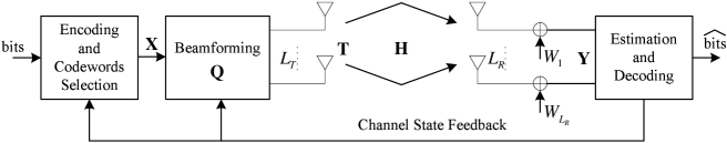
Figure 1: System model

A communication system with $L_{T}$-transmit antennas and $L_{R}$-receive antennas is shown in Fig. 1. Let $\mathbf{T}\in\mathbb{C}^{L_{T}\times 1}$ be the transmitted signal, $\mathbf{Y}\in\mathbb{C}^{L_{R}\times 1}$ be the received signal, $\mathbf{H}\in\mathbb{C}^{L_{R}\times L_{T}}$ be the channel state matrix and $\mathbf{Z}\in\mathbb{C}^{L_{R}\times 1}$ be the Gaussian noise with zero mean. The system model can be expressed as

$$\mathbf{Y}=\mathbf{HT}+\mathbf{Z}$$

where $\mathrm{E}\left[\mathbf{Z}\mathbf{Z}^{\dagger}\right]=\mathbf{I}_{L_{R}}$. In this paper, the Rayleigh flat fading channel is considered: the entries of $\mathbf{H}$ are independent and identically distributed (i.i.d.) circularly symmetric complex Gaussian variables with zero mean and unit variance ($\mathcal{CN}\left(0,1\right)$) and $\mathbf{H}$ is i.i.d. for each channel use. At the beginning of each channel use, the channel state $\mathbf{H}$ is assumed to be perfectly estimated at the receiver, then quantized to finite bits and fed back to the transmitter through a feedback channel. The feedback channel is assumed to be error-free and zero-delay. The rate of the feedback is up to $R_{\mathrm{fb}}$ bits/channel use. After receiving the channel state feedback, the transmitter transmits the encoded signal according to the current feedback.

The general design problem for finite rate channel state feedback is difficult to solve. It is well known that the optimal transmitted signal should be circular symmetric Gaussian signal with zero mean and covariance matrix adapted according to the feedback [3]. Define the covariance matrix of the transmitted signal as $\mathbf{\Sigma}\triangleq E\left[\mathbf{T}\mathbf{T}^{\dagger}\right]$, the codebook of the covariance matrices as

$$\mathcal{B}_{\mathbf{\Sigma}}=\left\{\mathbf{\Sigma}_{i}\in\mathbb{C}^{L_{T}\times L_{T}}:\;1\leq i\leq 2^{R_{\mathrm{fb}}}\right\}$$

and the feedback function $\varphi\left(\cdot\right)$ as a mapping from the space of $\mathbf{H}$ to a index set $\left\{i:\;1\leq i\leq 2^{R_{\mathrm{fb}}}\right\}$. The corresponding optimization problem is to find the optimal codebook $\mathcal{B}_{\mathbf{\Sigma}}$ and the optimal feedback function $\varphi\left(\cdot\right)$ to maximize the information rate

$$\underset{\mathcal{B}_{\mathbf{\Sigma}}}{\max}\;\underset{\varphi\left(\cdot\right)}{\max}\;\mathrm{E}_{\mathbf{H}}\left[\mathrm{ln}\left|\mathbf{I}+\mathbf{H\Sigma}_{\varphi\left(\mathbf{H}\right)}\mathbf{H}^{\dagger}\right|\right],$$

with the average power constraint $\rho$

$$\mathrm{E}_{\mathbf{H}}\left[\mathrm{tr}\left(\mathbf{\Sigma}_{\varphi\left(\mathbf{H}\right)}\right)\right]\leq\rho.$$

It has been shown in [3] that the design of covariance codebook and the design of feedback function are two coupled optimization problems and difficult to solve.

To obtain analytic solution that reflects the influence of feedback rate on the information rate, we simplify the general problem to suboptimal power on/off strategy (with beamforming). In the later parts of this paper, we’ll show that power on/off strategy is near optimal. Denote the singular value decomposition of the covariance matrix as $\mathbf{\Sigma}=\mathbf{QPQ}^{\dagger}$ where the matrices $\mathbf{Q}$ and $\mathbf{P}$ are called as beamforming matrix and power control matrix respectively. Describe the column vectors of $\mathbf{Q}$ as beams. Name the beam corresponding to a positive power as an on-beam. The statistics of the transmitted signal is uniquely determined by the on-beams and the power on them. In our power on/off model, every on-beam corresponds to a constant power $P_{\mathrm{on}}$. The transmitted Gaussian signal $\mathbf{T}$ can be expressed as

$$\mathbf{T} = \mathbf{QX}$$

where $\mathbf{X}$ is random Gaussian vector with zero mean and covariance matrix $P_{\mathrm{on}}\mathbf{I}_{s}$, $s$ is the number of on-beams and the beamforming matrix $\mathbf{Q}\in\mathbb{C}^{L_{T}\times s}$ is composed of the $s$ on-beams and satisfies $\mathbf{Q}^{\dagger}\mathbf{Q}=\mathbf{I}_{s}$. The system model for power on/off strategy is given by

$$\mathbf{Y} = \mathbf{HQX}+\mathbf{Z}.$$

The optimization problem for power on/off strategy is stated in Problem 1. Since the number of on-beams $s$ is the rank of the beamforming matrix $\mathbf{Q}$, the feedback only needs to specify $\mathbf{Q}$. Denote the codebook of beamforming matrices as $\mathcal{B}=\left\{\mathbf{Q}_{i}\in\mathbb{C}^{L_{T}\times s}:\;\mathbf{Q}_{i}^{\dagger}\mathbf{Q}_{i}=\mathbf{I}_{s},\;0\leq s\leq L_{T},\;1\leq i\leq 2^{R_{\mathrm{fb}}}\right\}$. The feedback function is a mapping from the space of $\mathbf{H}$ to the index set $\left\{i:\;1\leq i\leq 2^{R_{\mathrm{fb}}}\right\}$.

Problem 1

(Power On/Off Strategy Design Problem) Find the optimal beamforming codebook $\mathcal{B}$, feedback function $\varphi\left(\cdot\right)$ and $P_{\mathrm{on}}$ to maximize the information rate,

$$\underset{P_{\mathrm{on}}}{\max}\;\underset{\mathcal{B}}{\max}\;\underset{\varphi\left(\cdot\right)}{\max\;}\mathrm{E}_{\mathbf{H}}\left[\mathrm{ln}\left|\mathbf{I}+P_{\mathrm{on}}\mathbf{HQ}_{\varphi\left(\mathbf{H}\right)}\mathbf{Q}_{\varphi\left(\mathbf{H}\right)}^{\dagger}\mathbf{H}^{\dagger}\right|\right],$$

with the average power constraint

$$\mathrm{E}_{\mathbf{H}}\left[P_{\mathrm{on}}\mathrm{tr}\left(\mathbf{Q}_{\varphi\left(\mathbf{H}\right)}\mathbf{Q}_{\varphi\left(\mathbf{H}\right)}^{\dagger}\right)\right]=P_{\mathrm{on}}\mathrm{E}_{\mathbf{H}}\left[s\right]\leq\rho,$$

where $s=s\left(\mathbf{H}\right)=\mathrm{rank}\left(\mathbf{Q}_{\varphi\left(\mathbf{H}\right)}\right)$ is the number of on-beams for a channel realization $\mathbf{H}$.

As we will show later, the power on/off assumption is the key to decouple the beamforming codebook design and feedback function design.

II-B Random Matrix Theory

In this subsection, we review relevant results on the spectra of large random matrices. Recall that $\mathbf{H}$ is an $L_{R}\times L_{T}$ random matrix with i.i.d. complex Gaussian entries with zero mean and unit variance. Define $m\triangleq\min\left\{L_{T},L_{R}\right\}$ and $n\triangleq\max\left\{L_{T},L_{R}\right\}$. Define

$$\mathbf{W}\triangleq\left\{\begin{array}[]{cc}\frac{1}{m}\mathbf{H}\mathbf{H}^{\dagger}&\mathrm{if}\;L_{R}<L_{T}\\ \frac{1}{m}\mathbf{H}^{\dagger}\mathbf{H}&\mathrm{if}\;L_{R}\geq L_{T}\end{array}\right..$$

Let $\left\{\lambda_{i}\right\}$ be the set of the eigenvalues of $\mathbf{W}$. Define the empirical eigenvalue distribution of $\mathbf{W}$ as

$$F\left(\lambda\right)\triangleq\frac{1}{m}\left|\left\{j:\;\lambda_{j}<\lambda\right\}\right|.$$

Then as $m$ and $n$ approach infinity simultaneously with $\tau\triangleq\frac{n}{m}$ fixed,

$$\underset{\left(n,m\right)\rightarrow\infty}{\lim}\frac{dF\left(\lambda\right)}{d\lambda}=\left\{\begin{array}[]{ll}\frac{1}{2\pi\lambda}\sqrt{\left(\lambda^{+}-\lambda\right)\left(\lambda-\lambda^{-}\right)}&\mathrm{for}\;\lambda\in\left[\lambda^{-},\lambda^{+}\right]\\ 0&\mathrm{otherwise}\end{array}\right.$$ (3)

almost surely where $\lambda^{\pm}=\left(\sqrt{\tau}\pm 1\right)^{2}$ [37]. Furthermore, consider a spectral statistical function with the form

$$g\left(\mathbf{W}\right)=\frac{1}{m}\sum_{i=1}^{m}g\left(\lambda_{i}\right).$$

If $g$ is continuous and bounded on $\left[\lambda^{-},\lambda^{+}\right]$, then

$$\underset{\left(n,m\right)\rightarrow\infty}{\lim}g\left(\mathbf{W}\right) = \int g\left(\lambda\right)dF\left(\lambda\right)$$ (4)

almost surely [7, 8, 37].

II-C Stiefel and Grassmann Manifolds

Stiefel manifold and Grassmann manifold are the geometric objects relevant to the beamforming codebook design. The Stiefel manifold $\mathcal{S}_{L_{T},s}\left(\mathbb{C}\right)$ (where $L_{T}\geq s$) is the set of all complex unitary $L_{T}\times s$ matrices $\mathcal{S}_{L_{T},s}\left(\mathbb{C}\right)=\left\{\mathbf{Q}\in\mathbb{C}^{L_{T}\times s}:\;\mathbf{Q}^{\dagger}\mathbf{Q}=\mathbf{I}_{s}\right\}$. Define an equivalence relation on the Stiefel manifold, i.e., two matrices $\mathbf{P},\mathbf{Q}\in\mathcal{S}_{L_{T},s}\left(\mathbb{C}\right)$ are equivalent if their column vectors span the same subspace. The Grassmann manifold $\mathcal{G}_{L_{T},s}\left(\mathbb{C}\right)$ is defined as the quotient space of $\mathcal{S}_{L_{T},s}\left(\mathbb{C}\right)$ with respect to this equivalent relation. It can also be viewed as the set of all the $s$-dimensional planes through the origin in the $L_{T}$-dimensional Euclidean space [38, 39]. A generator matrix $\mathbf{Q}\in\mathcal{S}_{L_{T},s}\left(\mathbb{C}\right)$ for an $s$-plane $\mathcal{Q}\in\mathcal{G}_{L_{T},s}\left(\mathbb{C}\right)$ is defined as the matrix whose columns span $\mathcal{Q}$. The generator matrix is not unique. If $\mathbf{Q}$ is a generator matrix for an $s$-dimensional plane $\mathcal{Q}\in\mathcal{G}^{L_{T},s}\left(\mathbb{C}\right)$, then $\mathbf{QU}$ with $\mathbf{U}\in\mathcal{S}_{s,s}$ is also a generator matrix of the same plane $\mathcal{Q}$ [38].

This paper considers the projection Frobenius metric (chordal distance) on the Grassmann manifold because it is relevant to the the performance analysis of power on/off strategy. The chordal distance between two $s$-planes $\mathcal{Q}_{1},\mathcal{Q}_{2}\in\mathcal{G}_{L_{T},s}\left(\mathbb{C}\right)$ can be defined by their generator matrices,

$$d_{c} \triangleq \frac{1}{\sqrt{2}}\left\|\mathbf{Q}_{1}\mathbf{Q}_{1}^{\dagger}-\mathbf{Q}_{2}\mathbf{Q}_{2}^{\dagger}\right\|_{F}$$ (5)

$$= =s-\mathrm{trace}\left(\left(\mathbf{Q}_{1}^{\dagger}\mathbf{Q}_{2}\right)\left(\mathbf{Q}_{1}^{\dagger}\mathbf{Q}_{2}\right)^{\dagger}\right),$$

where $\mathbf{Q}_{1}$ and $\mathbf{Q}_{2}$ are the generator matrices of $\mathcal{Q}_{1}$ and $\mathcal{Q}_{2}$ respectively [38]. Since the chordal distance is independent with the choice of the generator matrices, it is well defined [38].

The invariant measure and the uniform distribution play a crucial role in the statistics on $\mathcal{S}_{L_{T},s}\left(\mathbb{C}\right)$ and $\mathcal{G}_{L_{T},s}\left(\mathbb{C}\right)$. Let $\mathcal{M}$ be a measurable set in $\mathcal{S}_{L_{T},s}\left(\mathbb{C}\right)$ or $\mathcal{G}_{L_{T},s}\left(\mathbb{C}\right)$, a measure $\zeta$ is called invariant if

$$\zeta\left(\mathbf{A}\mathcal{M}\right)=\zeta\left(\mathcal{M}\right)=\zeta\left(\mathcal{M}\mathbf{B}\right)$$

for arbitrary $L_{T}\times L_{T}$ unitary matrix $\mathbf{A}$ and $s\times s$ unitary matrix $\mathbf{B}$. The invariant probability measure defines the uniform distribution on $\mathcal{S}_{L_{T},s}\left(\mathbb{C}\right)$ or $\mathcal{G}_{L_{T},s}\left(\mathbb{C}\right)$ [40, 32].

III Power On/Off Strategy with Perfect Beamforming

To isolate the effect of power on/off from the effect of imperfect beamforming, this section discusses the perfect beamforming case. The effect of imperfect beamforming will be treated in Section IV.

In this section and throughout, the following notations are used. Define $m=\min\left(L_{T},L_{R}\right)$ and $n=\max\left(L_{T},L_{R}\right)$. Define the normalized number of on-beams as $\bar{s}\triangleq\frac{1}{m}s$ and the normalized on-power as $\bar{P}_{\mathrm{on}}=mP_{\mathrm{on}}$. Define $\mathbf{W}\triangleq\frac{1}{m}\mathbf{HH}^{\dagger}$ if $L_{R}<L_{T}$ or $\mathbf{W}\triangleq\frac{1}{m}\mathbf{H}^{\dagger}\mathbf{H}$ if $L_{R}\geq L_{T}$. Denote the $i^{\mathrm{th}}$ largest eigenvalue of $\mathbf{W}$ by $\lambda_{i}$.

To analyze the perfect beamforming case, Section III-A describes the corresponding optimization problem, Section III-B solves the optimization problem by letting $L_{T}$ and $L_{R}$ approach infinity simultaneously, and Section III-C shows that the asymptotic solution is near optimal for MIMO systems with finite many antennas.

III-A The Design Problem with Perfect Beamforming

The definition for perfect beamforming is given as follows. Consider the singular value decomposition of the channel state matrix $\mathbf{H}=\mathbf{U\Lambda V}^{\dagger}$. Perfect beamforming means that for $\forall\mathbf{H}\in\mathbb{C}^{L_{R}\times L_{T}}$ and $1\leq s\leq L_{T}$, there exists $\mathbf{Q}\in\mathcal{B}$ such that the $s$ columns of the beamforming matrix $\mathbf{Q}\in\mathbb{C}^{L_{T}\times s}$ are some columns of the right singular-vector matrix $\mathbf{V}$, i.e., $\mathbf{V}^{\dagger}\mathbf{Q}\in\mathbb{C}^{L_{T}\times s}$ is with elements either 1 or 0.

With perfect beamforming, the optimization problem can be simplified. Suppose that $P_{\mathrm{on}}$ and $s=s\left(\mathbf{H}\right)$ are given. For a channel realization $\mathbf{H}$, the optimal feedback beamforming matrix is $\mathbf{Q}_{\varphi\left(\mathbf{H}\right)}=\mathbf{V}_{s}$ where $\mathbf{V}_{s}$ is composed of the right singular vectors corresponding to the largest $s$ singular values of $\mathbf{H}$. Then, the mutual information between the transmitted signal and the received signal is

$$\mathcal{I}\left(\mathbf{H}\right) = \ln\left|\mathbf{I}_{L_{R}}+P_{\mathrm{on}}\mathbf{HQ}_{\varphi\left(\mathbf{H}\right)}\mathbf{Q}_{\varphi\left(\mathbf{H}\right)}^{\dagger}\mathbf{H}^{\dagger}\right|$$ (6)

$$= \sum_{i=1}^{s}\ln\left(1+\bar{P}_{\mathrm{on}}\lambda_{i}\right).$$

The corresponding optimization problem is stated as follows.

Problem 2

(Power On/Off Design with Perfect Beamforming) Find the optimal $s=s\left(\mathbf{H}\right)$ (or $\bar{s}=\bar{s}\left(\mathbf{H}\right)$) function and $P_{\mathrm{on}}$ (or $\bar{P}_{\mathrm{on}}$) to maximize the information rate,

$$\underset{P_{\mathrm{on}}}{\max}\;\underset{s\left(\cdot\right)}{\max}\;\mathrm{E}_{\mathbf{H}}\left[\sum_{i=1}^{s}\mathrm{ln}\left(1+\bar{P}_{\mathrm{on}}\lambda_{i}\right)\right],$$

with the power constraint

$$\mathrm{E}_{\mathbf{H}}\left[sP_{\mathrm{on}}\right]=\bar{P}_{\mathrm{on}}\mathrm{E}_{\mathbf{H}}\left[\bar{s}\right]\leq\rho.$$

The following theorem gives the form of the optimal $\bar{s}$ function to solve Problem 2.

Theorem 1

The optimal $\bar{s}$ function to solve Problem 2 is of the form

$$\bar{s}=\frac{1}{m}\left|\left\{k:\;\lambda_{k}\geq\kappa\right\}\right|$$ (7)

where $\kappa$ is the appropriate threshold chosen to satisfy the average power constraint

$$\bar{P}_{\mathrm{on}}\mathrm{E}_{\mathbf{H}}\left[\bar{s}\right]=\rho.$$

Proof:

See Appendix -A. ∎

The intuition behind the proof is that all the “good” beams (corresponding to $\lambda\geq\kappa$) and only the “good” beams should be turned on. This intuition will be used in the proof of Theorem 6 later.

Although the form of the optimal $\bar{s}$ function is given in (7), it is difficult to find the key parameters (the optimal $\bar{P}_{\mathrm{on}}$ and $\kappa$) and the corresponding information rate $\mathcal{I}$. Different from the water filling solution for CSITR case where the Lagrange multiplier is uniquely determined by $\rho$ [1], power on/off strategy has uncountable many pairs of $\bar{P}_{\mathrm{on}}$ and $\kappa$ corresponding to the same $\rho$. Numerical search may be employed to find the optimal $\bar{P}_{\mathrm{on}}$, $\kappa$ and the corresponding $\mathcal{I}$. However, if the numbers of transmit and receive antennas approach infinity simultaneously, as we will show in Section III-B, the corresponding key parameters and information rate can be explicitly computed.

III-B MIMO Systems with Infinitely Many Antennas

This section provides explicit formulas to solve Problem 2 by letting the numbers of transmit and receive antennas approach infinity simultaneously. As a byproduct of the employed method, this section also presents asymptotic formulas for the capacity of CSITR case. According to the authors knowledge, the derived asymptotic formulas are presented for the first time.

III-B1 Asymptotic Analysis for Power On/off Strategy

The main result of the asymptotic analysis is the following theorem, which gives the optimal $\bar{s}$ function when the numbers of transmit and receive antennas approach infinity simultaneously.

Theorem 2

Define $\tau\triangleq\frac{n}{m}$. For a given SNR $\rho$, if $m$ and $n$ approach infinity simultaneously with $\tau$ fixed, the optimal $\bar{s}$ function converges to a constant,

$$\bar{s}_{\infty}\triangleq\underset{\left(n,m\right)\rightarrow\infty}{\lim}\bar{s}=\int_{\kappa}^{\lambda^{+}}f\left(\lambda\right)d\lambda,$$

almost surely, and the corresponding normalized information rate $\bar{\mathcal{I}}\triangleq\frac{1}{m}\mathcal{I}$ also converges to a constant,

$$\bar{\mathcal{I}}_{\infty}\triangleq\underset{\left(n,m\right)\rightarrow\infty}{\lim}\bar{\mathcal{I}}=\int_{\kappa}^{\lambda^{+}}\mathrm{ln}\left(1+\frac{\rho}{\bar{s}_{\infty}}\lambda\right)f\left(\lambda\right)d\lambda,$$ (8)

where

$$f\left(\lambda\right) = \frac{1}{2\pi\lambda}\sqrt{\left(\lambda^{+}-\lambda\right)\left(\lambda-\lambda^{-}\right)},$$

$\lambda^{\pm}\triangleq\left(\sqrt{\tau}\pm 1\right)^{2}$ and $\lambda^{+}>\kappa\geq\lambda^{-}$ is the appropriate constant chosen to maximize the normalized information rate (8).

Proof:

Recall the optimal $\bar{s}$ function in (7). According to (3) in Section II-B,

$$\underset{\left(n,m\right)\rightarrow\infty}{\lim}\bar{s} = \underset{\left(n,m\right)\rightarrow\infty}{\lim}\frac{1}{m}\left|\left\{k:\;\lambda_{k}\geq\kappa\right\}\right|$$

$$= \underset{\left(n,m\right)\rightarrow\infty}{\lim}1-F\left(\lambda\right)$$

$$= \int_{\kappa}^{\lambda^{+}}f\left(\lambda\right)d\lambda$$

almost surely.

For any positive constant $\bar{P}_{\mathrm{on}}$ and a channel realization $\mathbf{H}$, according to the random matrix theory in (4), the normalized mutual information between the transmitted signal and the received signal converges to a constant,

$$\underset{\left(n,m\right)\rightarrow\infty}{\lim}\bar{\mathcal{I}}\left(\mathbf{H}\right) = \underset{\left(n,m\right)\rightarrow\infty}{\lim}\frac{1}{m}\sum_{i=1}^{s}\mathrm{ln}\left(1+\bar{P}_{\mathrm{on}}\lambda_{i}\right)$$

$$= \int_{\kappa}^{\lambda^{+}}\mathrm{ln}\left(1+\bar{P}_{\mathrm{on}}\lambda\right)f\left(\lambda\right)d\lambda,$$

almost surely. Thus the normalized information rate converges to a constant

$$\underset{\left(n,m\right)\rightarrow\infty}{\lim}\bar{\mathcal{I}} = \underset{\left(n,m\right)\rightarrow\infty}{\lim}\mathrm{E}_{\mathbf{H}}\left[\bar{\mathcal{I}}\left(\mathbf{H}\right)\right]$$

$$= \int_{\kappa}^{\lambda^{+}}\mathrm{ln}\left(1+\bar{P}_{\mathrm{on}}\lambda\right)f\left(\lambda\right)d\lambda.$$

Furthermore, an elementary calculation shows that the choice of $\bar{P}_{\mathrm{on}}=\rho/\bar{s}_{\infty}$ satisfies the average power constraint. Therefore, we have

$$\bar{\mathcal{I}}_{\infty}=\underset{\left(n,m\right)\rightarrow\infty}{\lim}\bar{\mathcal{I}}=\int_{\kappa}^{\lambda^{+}}\mathrm{ln}\left(1+\frac{\rho}{\bar{s}_{\infty}}\lambda\right)f\left(\lambda\right)d\lambda.$$

Finally, $\bar{s}_{\infty}$, $\bar{P}_{\mathrm{on}}$ and $\bar{\mathcal{I}}_{\infty}$ are all functions of $\kappa$, the optimization problem is to choose appropriate $\kappa$ to maximize $\bar{\mathcal{I}}_{\infty}$. ∎

This theorem proves that the optimal normalized number of on-beams $\bar{s}$ converges to a constant independent of the specific channel realization for a given SNR requirement. The principle behind this theorem is same as that of channel hardening [41]: the characteristic of a MIMO channel turns to be deterministic as the numbers of transmit and receive antennas approach infinity.

To find explicit formulas to calculate the key parameters and the corresponding performance, we need the following variable change

$$\lambda\left(t\right)=\frac{1}{y}\left(1+y-2\sqrt{y}\mathrm{cos}\left(t\right)\right),$$ (9)

where $y\triangleq\frac{m}{n}=\frac{1}{\tau}$ and $t\in\left[0,\pi\right]$. After the variable change, the asymptotic empirical density function of $t$ can be written as

$$f_{T}\left(t\right)=\left\{\begin{array}[]{ll}\frac{1}{\pi}\cdot\frac{1-\cos\left(2t\right)}{1+y-2\sqrt{y}\cos\left(t\right)}&\mathrm{if}\;y<1\\ \frac{1+\cos\left(t\right)}{\pi}&\mathrm{if}\;y=1\end{array}\right.$$ (12)

Define $a$ such that $\lambda\left(a\right)=\kappa$ where $\kappa$ is the optimal threshold in Theorem 2. Then we have the following corollary according to Theorem 2.

Corollary 1

If $m$ and $n$ approach infinity simultaneously with $y\triangleq\frac{m}{n}$ fixed, the optimal $\bar{s}$ function converges to a constant,

$$\bar{s}_{\infty}=\underset{\left(n,m\right)\rightarrow\infty}{\lim}\bar{s}=\int_{a}^{\pi}f_{T}\left(t\right)dt,$$ (13)

almost surely and the corresponding $\bar{\mathcal{I}}$ converges to a constant,

$$\bar{\mathcal{I}}_{\infty}=\underset{\left(n,m\right)\rightarrow\infty}{\lim}\bar{\mathcal{I}}=\int_{a}^{\pi}\ln\left(1+\frac{\rho}{y\bar{s}}\left(1+y-2\sqrt{y}\cos\left(t\right)\right)\right)f_{T}\left(t\right)dt,$$ (14)

where $a\in\left[0,\pi\right]$ is chosen to maximize the normalized information rate (14).

Since the variable change (9) is invertible, to find the optimal $\kappa$ in Theorem 2 is equivalent to find the optimal $a$ in Corollary 1. The following theorem gives a method to find the optimal $a$.

Theorem 3

If $m$ and $n$ approach infinity simultaneously with $y\triangleq\frac{m}{n}$ fixed, then $\frac{d\bar{\mathcal{I}}_{\infty}}{da}=0$ has at most one solution in the domain of $\left(0,\pi\right)$. The optimal $a$ to maximize $\bar{\mathcal{I}}_{\infty}$ is either the unique solution of $\frac{d\bar{\mathcal{I}}_{\infty}}{da}=0$ in $\left(0,\pi\right)$ if it exists, or 0 if $\frac{d\bar{\mathcal{I}}_{\infty}}{da}\neq 0$ for all $a\in\left(0,\pi\right)$.

Proof:

See Appendix -B. ∎

The following corollaries show how the optimal $a$ and the optimal $\bar{s}_{\infty}$ change when the average power constraint $\rho$ increases. The results will be applied to MIMO systems with finite many antennas in Section III-C.

Corollary 2

If $m$ and $n$ approach infinity simultaneously with $y\triangleq\frac{m}{n}$ fixed, the optimal $a$ to maximize $\bar{\mathcal{I}}_{\infty}$ is a non-increasing function of $\rho$.

Proof:

See Appendix -C. ∎

Corollary 3

If $m$ and $n$ approach infinity simultaneously with $y\triangleq\frac{m}{n}$ fixed, the optimal number of on-beams $\bar{s}_{\infty}$ to maximize $\bar{\mathcal{I}}_{\infty}$ is a nondecreasing function of $\rho$.

Proof:

Note that $\bar{s}_{\infty}=\int_{a}^{\pi}f_{T}\left(t\right)dt$ which is a monotone decreasing function of $a$. This corollary follows Corollary 2. ∎

Based on the above asymptotic results, the design problem for perfect beamforming (Problem 2) can be solved. According to Theorem 3, the asymptotic optimal threshold, say $a_{\infty}$, can be found by checking $\frac{d\bar{\mathcal{I}}_{\infty}}{da}$. The corresponding optimal normalized number of on-beams $\bar{s}_{\infty}$ and the normalized information rate $\bar{\mathcal{I}}_{\infty}$ can be computed by substituting $a_{\infty}$ into (13) and (14) respectively.

However, the calculations involve integrals, which may be computational complex. To simplify the computation, Propositions 1-3 express the integrals as some special functions which are defined by infinite series. Generally, the calculation of the series is much easier than numerical integrals. To make the expressions clear, the following notations are used.

$$r\triangleq\sqrt{y},$$ (15)

$$\alpha\triangleq\frac{\bar{s}_{\infty}y}{\rho},$$ (16)

$$w\triangleq\frac{1}{2}\left(1+y+\alpha+\sqrt{\left(1+y+\alpha\right)^{2}-4y}\right),$$ (17)

$$u\triangleq\frac{1}{2r}\left(1+y+\alpha-\sqrt{\left(1+y+\alpha\right)^{2}-4y}\right),$$ (18)

$$\theta_{r}\triangleq\tan^{-1}\left(\frac{r\sin\left(a\right)}{1-r\cos\left(a\right)}\right),$$ (19)

for $r\cos\left(a\right)\neq 1$ and

$$\theta_{u}\triangleq\tan^{-1}\left(\frac{u\sin\left(a\right)}{1-u\cos\left(a\right)}\right),$$ (20)

for $u\cos\left(a\right)\neq 1$. There are also three special functions defined by series. The first one is called Dilogarithm in literature [42] and defined as

$$\mathrm{Li}_{2}\left(x\right)\triangleq\sum_{n=1}^{\infty}\frac{x^{n}}{n^{2}},$$ (21)

for $\left|x\right|\leq 1$. We define the other two as

$$\mathrm{Sr}_{1}\left(u,r,t\right)\triangleq\sum_{l=1}^{\infty}\frac{r^{l}e^{ilt}}{l}\left(\sum_{k=1}^{l-1}\frac{\left(\frac{u}{r}\right)^{k}}{k}+\frac{1}{r^{2l}}\sum_{k=l}^{\infty}\frac{r^{2k}\left(\frac{u}{r}\right)^{k}}{k}\right)$$ (22)

and

$$\mathrm{Sr}_{2}\left(r,t\right)\triangleq\sum_{l=1}^{\infty}\frac{r^{l}e^{ilt}}{l}\left(\frac{1}{r^{2l}}\sum_{k=l}^{\infty}\frac{r^{2k}}{k}\right)$$ (23)

for $\left|u\right|<1$, $\left|r\right|<1$ and $\left|\frac{u}{r}\right|<1$.

Proposition 1

If $m$ and $n$ approach infinity simultaneously with $y\triangleq\frac{m}{n}$ fixed, the normalized number of on-beams $\bar{s}_{\infty}$ (as a function of $a$) is given by

$$\bar{s}_{\infty}=\left\{\begin{array}[]{ll}\frac{1}{\pi}\left\{\pi-a-\frac{1}{r}\sin\left(a\right)+\frac{1-r^{2}}{r^{2}}\theta_{r}\right\}&\mathrm{if}\>y<1\\ \frac{1}{\pi}\left\{\pi-a-\sin\left(a\right)\right\}&\mathrm{if}\>y=1\end{array}\right..$$

Proof:

See Appendix -D. ∎

Proposition 2

If $m$ and $n$ approach infinity simultaneously with $y\triangleq\frac{m}{n}$ fixed, the normalized information rate $\bar{\mathcal{I}}_{\infty}$ (as a function of the threshold $a$) is given by

$$\bar{\mathcal{I}}_{\infty}=\left\{\begin{array}[]{ll}\left[\ln\left(w\right)-\ln\left(\alpha\right)\right]\bar{s}_{\infty}+J_{0}+J_{1}+J_{2}&\mathrm{if}\>y<1\\ \left[\ln\left(w\right)-\ln\left(\alpha\right)\right]\bar{s}_{\infty}+J_{0}+J_{1}&\mathrm{if}\>y=1\end{array}\right.$$

where

$$J_{0}=\frac{1}{\pi r}\left\{\sin\left(a\right)\left[1-\ln\left(1+u^{2}-2u\cos\left(a\right)\right)\right]-u\left(\pi-a\right)-\left(\frac{1}{u}-u\right)\theta_{u}\right\}$$

$$J_{1}=\frac{1+r^{2}}{2\pi r^{2}}i\left[\mathrm{Li}_{2}\left(ue^{-ia}\right)-\mathrm{Li}_{2}\left(ue^{ia}\right)\right]$$

and

$$J_{2}=\frac{1-r^{2}}{2\pi r^{2}}\left[-2\ln\left(1-ur\right)\left(\pi-a-\theta_{r}\right)+i\mathrm{Sr}_{1}\left(u,r,a\right)-i\mathrm{Sr}_{1}\left(u,r,-a\right)\right].$$

Proof:

See Appendix -E. ∎

Proposition 3

If $m$ and $n$ approach infinity simultaneously with $y\triangleq\frac{m}{n}$ fixed, $\frac{d\bar{\mathcal{I}}_{\infty}}{da}$ is given by

$$\frac{d\bar{\mathcal{I}}_{\infty}}{da}=\frac{J_{3}}{\pi}\cdot\left[1-\ln\left(1+\frac{\rho}{\bar{s}_{\infty}y}\left(1+r^{2}-2r\cos\left(a\right)\right)\right)-\frac{y}{\rho}I^{d}\right],$$

where

$$J_{3}=\left\{\begin{array}[]{ll}\frac{1-\cos\left(2a\right)}{1+r^{2}-2r\cos\left(a\right)}&\mathrm{if}\>y<1\\ 1+\cos\left(a\right)&\mathrm{if}\>y=1\end{array}\right.$$

and

$$I^{d}=\left\{\begin{array}[]{ll}\frac{1}{\pi w\left(1-ur\right)}\left[\pi-a-\frac{1-u^{2}}{u\left(r-u\right)}\theta_{u}+\frac{1-r^{2}}{r\left(r-u\right)}\theta_{r}\right]&\mathrm{if}\>y<1\\ \frac{\pi-a}{\pi w\left(1-u\right)}-\frac{\left(1+u\right)\theta_{u}}{\pi wu\left(1-u\right)}&\mathrm{if}\>y=1.\end{array}\right.$$

Proof:

See Appendix -F. ∎

Following the method in [7, 8], Proposition 1-3 provide close form formulas to evaluate $\bar{s}_{\infty}$, $\bar{\mathcal{I}}_{\infty}$ and $\frac{d\bar{\mathcal{I}}_{\infty}}{da}$. In [7, 8], the closed form of the capacity is derived for CSIR only case, where all $L_{T}$ available beams are turned on. The results in [7, 8] can be viewed as a special case of Proposition 2 where $a=0$.

III-B2 Asymptotic Analysis for CSITR Case

To compare power on/off strategy with water filling power control (corresponds to CSITR case), we present asymptotic formulas to evaluate the CSITR capacity. As far as the authors know, these asymptotic results are presented for the first time.

It is well known that water filling power control can achieve the capacity assuming perfect CSIT [1]. Let $m=\mathrm{min}\left(L_{R},L_{T}\right)$, $n=\mathrm{max}\left(L_{R},L_{T}\right)$, $\tau=\frac{n}{m}$. When $m$ and $n$ approach infinity simultaneously with the ratio $\tau$ fixed, according to (4), the normalized capacity is given by

$$\bar{C}_{\infty}\triangleq\underset{\left(m,n\right)\rightarrow\infty}{\lim}\;\frac{1}{m}C=\int_{\max\left(\lambda^{-},\frac{1}{\nu}\right)}^{\lambda^{+}}\mathrm{ln}\left(\lambda\nu\right)f\left(\lambda\right)d\lambda,$$

where $f\left(\lambda\right)=\frac{1}{2\pi\lambda}\sqrt{\left(\lambda^{+}-\lambda\right)\left(\lambda-\lambda^{-}\right)}$, $\lambda^{\pm}=\left(\sqrt{\tau}\pm 1\right)^{2}$ and $\nu$ is the Lagrange multiplier chosen to satisfy the average power constraint,

$$\rho=\int_{\max\left(\lambda^{-},\frac{1}{\nu}\right)}^{\lambda^{+}}\left(\nu-\frac{1}{\lambda}\right)f\left(\lambda\right)d\lambda.$$

To derive closed forms for the integrals, consider the same variable change as in (9). Then the asymptotic normalized capacity $\bar{C}_{\infty}$ is given by

$$\bar{C}_{\infty}=\int_{a}^{\pi}\mathrm{ln}\left(\frac{\nu}{y}\left(1+y-2\sqrt{y}\cos\left(t\right)\right)\right)f_{T}\left(t\right)dt,$$

where

$$a=\left\{\begin{array}[]{ll}\cos^{-1}\left(\frac{1+y-\frac{y}{\nu}}{2\sqrt{y}}\right)&\mathrm{if}\;\lambda^{-}\leq\frac{1}{\nu}\leq\lambda^{+}\\ 0&\mathrm{if}\;\frac{1}{\nu}<\lambda^{-}\end{array}\right.,$$

$\nu$ is the Lagrange multiplier chosen to satisfy the average power constraint

$$\rho=\int_{a}^{\pi}\left(\nu-\frac{y}{1+y-2\sqrt{y}\cos\left(t\right)}\right)f_{T}\left(t\right)dt,$$

and $f_{T}\left(t\right)$ is given in (12).

The following propositions give the closed forms for the average power and the normalized capacity as a function of $\nu$. To make the presentation clearer, the notations in (15-23) are used.

Proposition 4

If $m$ and $n$ approach infinity simultaneously with $y=\frac{m}{n}$ fixed, the relationship between the power constraint $\rho$ and the Lagrange multiplier $\nu$ is given by

$$\rho=\nu\bar{s}_{\infty}-J_{4},$$

where

$$\bar{s}_{\infty}=\int_{a}^{\pi}f_{T}\left(t\right)dt,$$

$$J_{4}=\left\{\begin{array}[]{ll}\frac{1}{\pi}\left[\frac{r^{2}}{1-r^{2}}\left(\pi-a\right)-\frac{1+r^{2}}{1-r^{2}}\theta_{r}+\frac{i}{2}\left(\frac{1}{1-re^{-ia}}-\frac{1}{1-re^{ia}}\right)\right]&\mathrm{if}\;y<1\\ \frac{1}{2\pi}\left[\pi-a-\frac{2}{\tan\left(\frac{a}{2}\right)}\right]&\mathrm{if}\;y=1\end{array}\right.$$

and

$$a=\left\{\begin{array}[]{ll}\cos^{-1}\left(\frac{1+y-\frac{y}{\nu}}{2\sqrt{y}}\right)&\mathrm{if}\;\lambda^{-}\leq\frac{1}{\nu}\leq\lambda^{+}\\ 0&\mathrm{if}\;\frac{1}{\nu}<\lambda^{-}\end{array}\right..$$

Proof:

See Appendix -G. ∎

Proposition 5

If $m$ and $n$ approach infinity simultaneously with $y=\frac{m}{n}$ fixed, the normalized capacity $\bar{C}_{\infty}$ is given by

$$\bar{C}_{\infty}=\left\{\begin{array}[]{ll}\ln\left(\frac{\nu}{y}\right)\bar{s}_{\infty}+J_{5}+J_{6}+J_{7}&\mathrm{if}\;y<1\\ \ln\left(\frac{\nu}{y}\right)\bar{s}_{\infty}+J_{5}+J_{6}&\mathrm{if}\;y=1\end{array}\right.,$$

where

$$\bar{s}_{\infty}=\int_{a}^{\pi}f_{T}\left(t\right)dt,$$

$$J_{5}=\frac{1}{\pi r}\left\{\sin\left(a\right)\left[1-\ln\left(1+r^{2}-2r\cos\left(a\right)\right)\right]-r\left(\pi-a\right)-\left(\frac{1}{r}-r\right)\theta_{r}\right\},$$

$$J_{6}=\frac{1+r^{2}}{2\pi r^{2}}i\left[\mathrm{Li}_{2}\left(re^{-ia}\right)-\mathrm{Li}_{2}\left(re^{ia}\right)\right],$$

$$J_{7} = -\frac{1-r^{2}}{2\pi r^{2}}\left\{\frac{i}{2}\left[\ln^{2}\left(1-re^{-ia}\right)-\ln^{2}\left(1-re^{ia}\right)\right]\right.$$

$$\left.+2\ln\left(1-r^{2}\right)\left(\pi-a-\theta_{r}\right)+i\left[\mathrm{Sr}_{2}\left(r,-a\right)-\mathrm{Sr}_{2}\left(r,a\right)\right]\right\},$$

and

$$a=\left\{\begin{array}[]{ll}\cos^{-1}\left(\frac{1+y-\frac{y}{\nu}}{2\sqrt{y}}\right)&\mathrm{if}\;\lambda^{-}\leq\frac{1}{\nu}\leq\lambda^{+}\\ 0&\mathrm{if}\;\frac{1}{\nu}<\lambda^{-}.\end{array}\right..$$

Proof:

See Appendix -H. ∎

Based on the above propositions, the Lagrange multiplier $\nu$ and the corresponding normalized capacity $\bar{C}_{\infty}$ can be easily computed for a given SNR requirement $\rho$.

III-C MIMO Systems with Finite Many Antennas

The asymptotic results in Section III-B can be applied to MIMO systems with finite many antennas. It is often the case that the asymptotic results are accurate enough for MIMO systems with finite many antennas [7, 37, 8, 43, 41]. So are the asymptotic results in Section III-B. Theorem 2 proves that the optimal normalized number of on-beams $\bar{s}$ converges to a constant asymptotically. We will show that a constant $\bar{s}$ is near optimal for MIMO systems with finite many antennas. Moreover, according to the asymptotic result in Corollary 3, the optimal $\bar{s}$ is a nondecreasing function as the average $\rho$ increases. It is consistent with the results in [20, 21], which consider the special case of transmit antenna selection and show that at most one beam should be turned on when $\rho$ is small enough and $m$ beams should be on when $\rho$ is sufficiently large. Importantly though, the results in this paper is more general.

Before applying the asymptotic results, however, it is worthy to note note the difference between the asymptotic case and the case of finite many antennas. In asymptotic case, $\bar{s}$ can be any rational number in $\left[0,1\right]$. On the other hand, in the case of finite many antennas, $\bar{s}$ can only take finite many discrete values, $\bar{s}\in\left\{\frac{1}{m},\frac{2}{m},\cdots,1\right\}$ where $m=\min\left(L_{R},L_{T}\right)$ is the dimension of the MIMO system.

To apply the asymptotic results to the finite case, we use the following procedure.

1. For a given MIMO system with $L_{T}$-transmit antennas and $L_{R}$-receive antennas, define $m=\min\left(L_{R},L_{T}\right)$, $n=\max\left(L_{R},L_{T}\right)$ and $y=\frac{m}{n}$. According to the asymptotic analysis and formulas in Section III-B, evaluate the asymptotic optimal threshold $a_{\infty}$ and the asymptotic optimal normalized number of on-beams $\bar{s}_{\infty}$ for a given average SNR requirement $\rho$.

2. If $\bar{s}_{\infty}<\frac{1}{m}$, then go to 3). Otherwise, we choose the optimal $\bar{s}$ as the one corresponding to the larger $\bar{\mathcal{I}}$ from the adjacent discrete values to $\bar{s}_{\infty}$. Specifically, let $\bar{s}_{1}=\frac{1}{m}\left\lceil m\bar{s}_{\infty}\right\rceil$ and $\bar{s}_{2}=\frac{1}{m}\left\lfloor m\bar{s}_{\infty}\right\rfloor$ where $\left\lceil\cdot\right\rceil$ denotes the ceil function and $\left\lfloor\cdot\right\rfloor$ represents the floor function. Compare the corresponding performance $\bar{\mathcal{I}}$ (evaluated by substituting the corresponding $a$ into the asymptotic formula for $\bar{\mathcal{I}}_{\infty}$ in Proposition 2) and choose the better one as the optimal $\bar{s}$. According the Theorem 2, the $m\bar{s}$ beams corresponding to the largest $m\bar{s}$ eigenvalues of $\mathbf{W}$ are always turned on independent of the specific channel state realization $\mathbf{H}$. The power on each on-beam is $P_{\mathrm{on}}=\frac{\rho}{m\bar{s}}$ and the corresponding $\bar{\mathcal{I}}$ can be evaluated by asymptotic formula for $\bar{\mathcal{I}}_{\infty}$.

3. If $\bar{s}_{\infty}<\frac{1}{m}$, then at most one beam should be turned on. Put $\bar{s}=\frac{1}{m}$ and $P_{\mathrm{on}}=\frac{\rho}{m\bar{s}_{\infty}}$. We turn on/off the strongest beam, which corresponds to the largest eigenvalue of $\mathbf{W}$, according to the following threshold test,

   $$\lambda_{1}\overset{\mathrm{on}}{\underset{\mathrm{off}}{\gtrless}}\kappa$$

   where $\kappa=\frac{1}{y}\left(1+y-2\sqrt{y}\cos\left(a_{\infty}\right)\right)$.

The power on/off strategy designed according to the above procedure is called power on/off strategy with a constant number of on-beams. When the given average SNR $\rho$ is large enough so that $\bar{s}_{\infty}\geq\frac{1}{m}$, a constant number of on-beams are turned on independent of the specific channel realization $\mathbf{H}$. The only exception happens when $\rho$ is so low that $\bar{s}_{\infty}\leq\frac{1}{m}$, where either the strongest beam is turned on, when $\lambda_{1}\geq\kappa$, or no beams is on, when $\lambda_{1}<\kappa$. Although this strategy is designed according to the asymptotic results, it is near-optimal for MIMO systems with finite many antennas according to the simulation results.

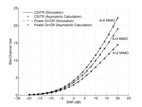
(a) Information rate

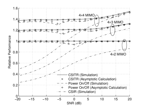
(b) Relative performance

Figure 2: Information rate v.s. SNR for perfect beamforming

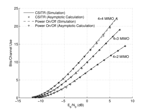
(a) Information rate

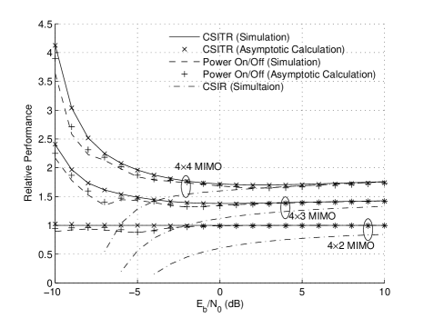
(b) Relative performance

Figure 3: Information rate v.s. $\mathrm{E_{b}/N_{0}}$ for perfect beamforming

Simulation results are given in Fig. 2 and Fig. 3. The information rate v.s. SNR is presented in Fig. 2(a) while Fig. 3(a) shows the information rate v.s. $\mathrm{E_{b}/N_{0}}$. Different MIMO systems with $4\times 2$, $4\times 3$ and $4\times 4$ antennas are considered. The solid line and the dashed line are the simulated information rate for CSITR case and power on/off strategy respectively. The “x” marker and the “+” marker are the information rate calculated according to asymptotic analysis for CSITR case and power on/off strategy respectively. The difference among them is almost unnoticeable. To make the performance difference clearer, we also define the relative performance as the ratio of the considered information rate and the capacity of a $4\times 2$ MIMO achieved by water filling power control with perfect CSITR. The relative performance for different MIMO systems is given in Fig. 2(b) and 3(b). The simulation results show that power on/off strategy (dashed lines) can achieve more than 90% of the capacity provided by water filling power control (solid lines) and has significant gain comparing to CSIR case (dash-dot lines) at low SNR. Note that there are several vales in the relative performance curves. This is due to the fact that $\bar{s}$ can only take discrete values. Furthermore, the performance evaluated by asymptotic analysis (“x” markers for CSITR case and “+” markers for power on/off strategy) is very close to the simulated performance. In conclusion, the power on/off strategy is near optimal for all SNR regimes and the corresponding performance can be well characterized by asymptotic analysis.

Since the asymptotic results are accurate for the finite many antennas case, we can also conclude that the information rate achieved by power on/off strategy or water filling power allocation grows linearly with the system dimension $m=\min\left(L_{R},L_{T}\right)$ for a given SNR. That is, for a given $L_{T}\times L_{R}$ MIMO system, the normalized information rate $\bar{\mathcal{I}}$ and the normalized capacity $\bar{C}$ are constants determined by the SNR $\rho$. The total information rate is that constant multiplied by the dimension $m$.

IV Power On/Off Strategy with a Finite Size Beamforming Codebook

This section is devoted to quantify the effect of imperfect beamforming due to finite rate feedback. Comparing to the capacity for perfect CSITR case, the performance loss of power on/off strategy with finite rate feedback comes from power on/off and imperfect beamforming. While Section III characterizes the information rate of power on/off strategy for perfect beamforming, this section will characterize the overall information rate by quantifying the effect of imperfect beamforming.

Recall the power on/off strategy optimization problem in Problem 1. Since the power on/off strategy with a constant number of on-beams is simple and near optimal, we focus on the effect of imperfect beamforming when the number of on-beams is a constant. For a constant number of on-beams, the beamforming codebook contains beamforming matrices of the same rank. Specifically, let the optimal number of on-beams be $s$ and the asymptotic optimal normalized number of on-beams be $\bar{s}_{\infty}$. When $\bar{s}_{\infty}\geq\frac{1}{m}$ (true for most SNR regimes),

$$\mathcal{B}=\left\{\mathbf{Q}_{i}\in\mathbb{C}^{L_{T}\times s}:\;\mathbf{Q}_{i}^{\dagger}\mathbf{Q}_{i}=\mathbf{I}_{s},\;1\leq i\leq 2^{R_{\mathrm{fb}}}\right\}.$$

The only exception happens when the required SNR is so low that $\bar{s}_{\infty}<\frac{1}{m}$ (see Section III-C for details), where the codebook contains beamforming vectors and one extra index for the case that the transmitter is turned off. In this case,

$$\mathcal{B}=\left\{\mathbf{Q}_{i}\in\mathbb{C}^{L_{T}\times 1}:\;\mathbf{Q}_{i}^{\dagger}\mathbf{Q}_{i}=1,\;1\leq i\leq 2^{R_{\mathrm{fb}}}-1\right\}\cup\left\{\mathbf{Q}_{\phi}\right\}$$

where $\mathbf{Q}_{\phi}$ is the artificial notation for the the case that the transmitter is turned off (no beam is on). Since there is no beamforming when no beam is on, the matrix $\mathbf{Q}_{\phi}$ has no effect in the analysis of imperfect beamforming. Thus the effect of imperfect beamforming can be analyzed for

$$\mathcal{B}=\left\{\mathbf{Q}_{i}\in\mathbb{C}^{L_{T}\times 1}:\;\mathbf{Q}_{i}^{\dagger}\mathbf{Q}_{i}=1,\;1\leq i\leq 2^{R_{\mathrm{fb}}}-1\right\},$$

which can be viewed as a codebook containing $2^{R_{\mathrm{fb}}}-1$ beamforming matrices of rank $1$. Call a beamforming codebook containing beamforming matrices of the same rank as a single rank beamforming codebook. The power on/off strategy optimization problem (Problem 1) is simplified to design a single rank beamforming codebook $\mathcal{B}$ with size $2^{R_{\mathrm{fb}}}$ or $2^{R_{\mathrm{fb}}}-1$ and the corresponding feedback function $\varphi\left(\cdot\right)$ to maximize the corresponding information rate.

To solve the optimization problem and make the performance analysis tractable, an asymptotic optimal feedback function is introduced and discussed in Section IV-A. The effect of a single rank beamforming codebook with this asymptotic optimal feedback function is well characterized in Section IV-B.

IV-A Feedback Function

This subsection considers the feedback function for a given single rank beamforming codebook.

The optimal feedback function is given as follows. When the number of on-beams is a constant $s$, the transmitter transmits a constant power $sP_{\mathrm{on}}$. For a given single rank beamforming codebook, it is easy to verify that the optimal feedback function $\varphi^{*}\left(\cdot\right)$ is given by

$$\varphi^{*}\left(\mathbf{H}\right)=\arg\;\underset{1\leq i\leq\left|\mathcal{B}\right|}{\max}\;\ln\left(I_{L_{R}}+P_{\mathrm{on}}\mathbf{HQ}_{i}\mathbf{Q}_{i}^{\dagger}\mathbf{H}^{\dagger}\right).$$

However, this paper considers a suboptimal but asymptotic optimal feedback function because the corresponding performance can be well analyzed. Consider the singular value decomposition that $\mathbf{H}=\mathbf{U\Lambda V}^{\dagger}$. Define $\mathbf{V}_{s}$ as the $L_{T}\times s$ matrix composed by the singular vectors in $\mathbf{V}$ corresponding to the largest $s$ singular values. Then both $\mathbf{V}_{s}$ and a beamforming matrix $\mathbf{Q}\in\mathcal{B}$ can be viewed as generator matrices of $s$-planes in Grassmann manifold $\mathcal{G}_{L_{T},s}\left(\mathbb{C}\right)$ (see Section II-C for relative definitions). Denote the planes generated by $\mathbf{V}_{s}$ and $\mathbf{Q}$ as $\mathcal{P}\left(\mathbf{V}_{s}\right)$ and $\mathcal{P}\left(\mathbf{Q}\right)$ respectively. The feedback function $\hat{\varphi}\left(\cdot\right)$ is defined as

$$\hat{\varphi}\left(\mathbf{H}\right) \triangleq \arg\;\underset{1\leq i\leq\left|\mathcal{B}\right|}{\min}\;d_{c}\left(\mathcal{P}\left(\mathbf{Q}_{i}\right),\mathcal{P}\left(\mathbf{V}_{s}\right)\right)$$ (32)

$$= \arg\;\underset{1\leq i\leq\left|\mathcal{B}\right|}{\max}\;\mathrm{tr}\left(\left(\mathbf{V}_{s}^{\dagger}\mathbf{Q}_{i}\right)\left(\mathbf{V}_{s}^{\dagger}\mathbf{Q}_{i}\right)^{\dagger}\right),$$

where $d_{c}$ is the chordal distance between two elements in $\mathcal{G}_{L_{T},s}\left(\mathbb{C}\right)$.

The feedback function (32) is asymptotic optimal. When the size of $\mathcal{B}$ approaches infinity, the beamforming codebook $\mathcal{B}$ can be constructed so that the chordal distance between $\mathcal{P}\left(\mathbf{Q}_{\hat{\varphi}\left(\mathbf{H}\right)}\right)$ and $\mathcal{P}\left(\mathbf{V}_{s}\right)$ approaches zero for any given $\mathbf{V}_{s}$. The information rate achieved by the suboptimal feedback function approaches that of perfect beamforming, which is also the limit that the optimal feedback strategy can achieve.

Theorem 4 shows a nice property of the asymptotic feedback strategy, which will be used to quantify the effect of a given single rank beamforming codebook in Section IV-B. The following lemma is used in the proof of Theorem 4.

Lemma 1

Let $\mathbf{A}\in\mathbb{C}^{k\times k}$ be a Hermitian matrix. If $\mathbf{A}=\mathbf{UA}\mathbf{U}^{\dagger}$ for any $k\times k$ unitary matrix $\mathbf{U}$, then $\mathbf{A}=\mu\mathbf{I}$ for some constant $\mu\in\mathbb{R}$.

Proof:

For any Hermitian $\mathbf{A}$, there exists a $k\times k$ unitary $\mathbf{U}$ such that $\mathbf{UA}\mathbf{U}^{\dagger}=\mathbf{\Lambda}$ where $\mathbf{\Lambda}$ is diagonal and with real diagonal elements. But $\mathbf{UA}\mathbf{U}^{\dagger}=\mathbf{A}$, then $\mathbf{A}$ is diagonal and real. Furthermore, put $\mathbf{U}$ as a permutation matrix, it is easy to verify that the diagonal elements are identical. ∎

Theorem 4

Let $\mathcal{B}$ be a single rank beamforming codebook with rank $s$ where $1\leq s\leq L_{T}$. Let $\mathbf{V}_{s}$ be a random matrix uniformly distributed on the Stiefel manifold $\mathcal{S}_{L_{T},s}\left(\mathbb{C}\right)$. Let

$$\hat{\varphi}\left(\mathbf{V}_{s}\right)=\arg\;\underset{1\leq i\leq\left|\mathcal{B}\right|}{\min}\;d_{c}\left(\mathcal{P}\left(\mathbf{Q}_{i}\right),\mathcal{P}\left(\mathbf{V}_{s}\right)\right).$$

Then

$$E_{\mathbf{V}_{s}}\left[\mathbf{V}_{s}^{\dagger}\mathbf{Q}_{\hat{\varphi}\left(\mathbf{V}_{s}\right)}\mathbf{Q}_{\hat{\varphi}\left(\mathbf{V}_{s}\right)}^{\dagger}\mathbf{V}_{s}\right]=\mu\mathbf{I}$$

where

$$\mu\triangleq 1-\frac{1}{s}E_{\mathbf{V}_{s}}\left[d_{c}^{2}\left(\mathcal{P}\left(\mathbf{Q}_{\hat{\varphi}\left(\mathbf{V}_{s}\right)}\right),\mathcal{P}\left(\mathbf{V}_{s}\right)\right)\right]$$

is a non-negative constant.

Proof:

For any $s\times s$ unitary matrix $\mathbf{U}$,

$$\mathbf{Q}_{\hat{\varphi}\left(\mathbf{V}_{s}\mathbf{U}\right)} = \arg\;\underset{1\leq i\leq\left|\mathcal{B}\right|}{\max}\;\mathrm{tr}\left(\left(\mathbf{Q}_{i}^{\dagger}\mathbf{V}_{s}\mathbf{U}\right)^{\dagger}\left(\mathbf{Q}_{i}^{\dagger}\mathbf{V}_{s}\mathbf{U}\right)\right)$$

$$= \arg\;\underset{1\leq i\leq\left|\mathcal{B}\right|}{\max}\;\mathrm{tr}\left(\left(\mathbf{Q}_{i}^{\dagger}\mathbf{V}_{s}\right)^{\dagger}\left(\mathbf{Q}_{i}^{\dagger}\mathbf{V}_{s}\right)\right)$$

$$= \mathbf{Q}_{\hat{\varphi}\left(\mathbf{V}_{s}\right)}.$$

Since $\mathbf{V}_{s}$ is uniformly distributed on $\mathcal{S}_{L_{T},s}\left(\mathbb{C}\right)$, $\mathbf{V}_{s}\mathbf{U}$ is uniformly distributed on $\mathcal{S}_{L_{T},s}\left(\mathbb{C}\right)$ as well [40]. Then,

$$\mathbf{U}^{\dagger}E_{\mathbf{V}_{s}}\left[\mathbf{V}_{s}^{\dagger}\mathbf{Q}_{\hat{\varphi}\left(\mathbf{V}_{s}\right)}\mathbf{Q}_{\hat{\varphi}\left(\mathbf{V}_{s}\right)}^{\dagger}\mathbf{V}_{s}\right]\mathbf{U}$$

$$=E_{\mathbf{V}_{s}}\left[\mathbf{U}^{\dagger}\mathbf{V}_{s}^{\dagger}\mathbf{Q}_{\hat{\varphi}\left(\mathbf{V}_{s}\right)}\mathbf{Q}_{\hat{\varphi}\left(\mathbf{V}_{s}\right)}^{\dagger}\mathbf{V}_{s}\mathbf{U}\right]$$

$$\overset{\left(a\right)}{=}E_{\mathbf{V}_{s}}\left[\left(\mathbf{V}_{s}\mathbf{U}\right)^{\dagger}\mathbf{Q}_{\hat{\varphi}\left(\mathbf{V}_{s}\mathbf{U}\right)}\mathbf{Q}_{\hat{\varphi}\left(\mathbf{V}_{s}\mathbf{U}\right)}^{\dagger}\left(\mathbf{V}_{s}\mathbf{U}\right)\right]$$

$$\overset{\left(b\right)}{=}E_{\mathbf{V}_{s}\mathbf{U}}\left[\left(\mathbf{V}_{s}\mathbf{U}\right)^{\dagger}\mathbf{Q}_{\hat{\varphi}\left(\mathbf{V}_{s}\mathbf{U}\right)}\mathbf{Q}_{\hat{\varphi}\left(\mathbf{V}_{s}\mathbf{U}\right)}^{\dagger}\left(\mathbf{V}_{s}\mathbf{U}\right)\right]$$

$$\overset{\left(c\right)}{=}E_{\mathbf{V}_{s}}\left[\mathbf{V}_{s}^{\dagger}\mathbf{Q}_{\hat{\varphi}\left(\mathbf{V}_{s}\right)}\mathbf{Q}_{\hat{\varphi}\left(\mathbf{V}_{s}\right)}^{\dagger}\mathbf{V}_{s}\right],$$

where

(a) follows from the fact that $\mathbf{Q}_{\hat{\varphi}\left(\mathbf{V}_{s}\mathbf{U}\right)}=\mathbf{Q}_{\hat{\varphi}\left(\mathbf{V}_{s}\right)}$,
(b) follows from the fact that $\mathbf{V}_{s}\mathbf{U}$ and $\mathbf{V}_{s}$ have the same distribution, and
(c) follows from the variable change from $\mathbf{V}_{s}\mathbf{U}$ to $\mathbf{V}_{s}$.

Therefore, $E_{\mathbf{V}_{s}}\left[\mathbf{V}_{s}^{\dagger}\mathbf{Q}_{\hat{\varphi}\left(\mathbf{V}_{s}\right)}\mathbf{Q}_{\hat{\varphi}\left(\mathbf{V}_{s}\right)}^{\dagger}\mathbf{V}_{s}\right]=\mu\mathbf{I}$ for some constant $\mu$ according to Lemma 1. The constant $\mu$ is non-negative because $\mathbf{V}_{s}^{\dagger}\mathbf{Q}_{\hat{\varphi}\left(\mathbf{V}_{s}\right)}\mathbf{Q}_{\hat{\varphi}\left(\mathbf{V}_{s}\right)}^{\dagger}\mathbf{V}_{s}$ is non-negative definite.

Furthermore, an elementary calculation shows that

$$\mu=1-\frac{1}{s}E_{\mathbf{V}_{s}}\left[d_{c}^{2}\left(\mathcal{P}\left(\mathbf{Q}_{\hat{\varphi}\left(\mathbf{V}_{s}\right)}\right),\mathcal{P}\left(\mathbf{V}_{s}\right)\right)\right].$$

∎

The constant $\mu$ in the above theorem is related to the average distortion (defined by squared chordal distance) of a quantization on the Grassmann manifold. Particularly, we are interested in the maximum $\mu$ achievable given a codebook size. This problem is solved in [36] and we state the result as the following.

Theorem 5

Let $\mathcal{B}$ be a single rank beamforming codebook with rank $s$ where $1\leq s\leq L_{T}$. Denote the size of $\mathcal{B}$ by $K$. Let $\mathcal{V}$ be a random plane uniformly distributed on the Grassmann manifold $\mathcal{G}_{L_{T},s}\left(\mathbb{C}\right)$. Define the average squared chordal distance as

$$\overline{d_{c}^{2}}\left(\mathcal{B}\right)\triangleq E_{\mathcal{V}}\left[\underset{\mathbf{Q}\in\mathcal{B}}{\min}\;d_{c}^{2}\left(\mathcal{P}\left(\mathbf{Q}\right),\mathcal{V}\right)\right].$$

The minimum average squared chordal distance achievable for a given $K$, say $\overline{d_{c}^{2}}_{\inf}$, is defined as

$$\overline{d_{c}^{2}}_{\inf}\triangleq\underset{\mathcal{B}:\;\left|\mathcal{B}\right|=K}{\inf}\;\overline{d_{c}^{2}}\left(\mathcal{B}\right).$$

Assume that $K$ is large. $\overline{d_{c}^{2}}_{\inf}$ can be bounded by

$$\frac{t}{t+1}\eta^{-\frac{1}{t}}2^{-\frac{\log_{2}K}{t}}\lesssim\overline{d_{c}^{2}}_{\inf}\lesssim\frac{\Gamma\left(\frac{1}{t}\right)}{t}\eta^{-\frac{1}{t}}2^{-\frac{\log_{2}K}{t}},$$ (33)

where $t=s\left(L_{T}-s\right)$ is the number of the real dimensions of $\mathcal{G}_{L_{T},s}\left(\mathbb{C}\right)$,

$$\eta=\left\{\begin{array}[]{ll}\frac{1}{t!}\prod_{i=1}^{s}\frac{\left(L_{T}-i\right)!}{\left(s-i\right)!}&\mathrm{if}\;1\leq s\leq\frac{L_{T}}{2}\\ \frac{1}{t!}\prod_{i=1}^{L_{T}-s}\frac{\left(L_{T}-i\right)!}{\left(L_{T}-s-i\right)!}&\mathrm{if}\;\frac{L_{T}}{2}\leq s\leq L_{T}\end{array}\right.,$$ (34)

and the symbol $\lesssim$ denotes the main order inequality.

Although this theorem is for asymptotically large $K$, the bounds (33) are accurate enough for relatively small $K$. For example, it is shown in [36] that the bounds are tight for $K\geq 10$ when $L_{T}=4$, $s=2$ . Furthermore, as the number of real dimensions of the Grassmann manifold ($2t$) approaches infinity, the lower bound and the upper bound are asymptotically equal.

It is noteworthy that Theorem 5 holds for Grassmann manifolds with arbitrary dimensions. In [31], approximations to $\bar{d}_{c,\inf}^{2}$ are developed for $s=1$ case and the case that $s\geq 1$ is fixed and $L_{T}$ is asymptotically large. Indeed, the approximation in [31] for $s=1$ is a lower bound on $\bar{d}_{c,\inf}^{2}$. The approximation in [31] for fixed $s$ and asymptotically large $L_{T}$ is neither a lower bound nor an upper bound. A detailed comparison of Theorem 5 and the results of [31] can be found in [36].

Apply Theorem 5 to Theorem 4, the maximum $\mu$ achievable, say $\mu_{\sup}$, can be upper and lower bounded. This result about the suboptimal feedback function will be employed to analyze the effect of a single rank beamforming codebook on information rate in Section IV-B.

IV-B Effect of a Beamforming Codebook

In this section, the effect of a single rank beamforming codebook is accurately quantified. Thus the overall performance of power on/off strategy with finite rate feedback can be well characterized by combining the asymptotic results in Section III and the effect of a single rank beamforming codebook.

A lower bound to the information rate is derived first. For a channel state realization $\mathbf{H}$, let $\lambda_{i}$ be the $i^{\mathrm{th}}$ largest eigenvalue of $\mathbf{H}^{\dagger}\mathbf{H}$ and $\mathbf{v}_{i}$ be the eigenvector corresponding to $\lambda_{i}$. Then $\mathbf{H}^{\dagger}\mathbf{H}=\mathbf{V\Lambda V}^{\dagger}$ where $\mathbf{V}=\left[\mathbf{v}_{1},\mathbf{v}_{2},\cdots,\mathbf{v}_{L_{T}}\right]$ and $\mathbf{\Lambda}=\mathrm{diag}\left[\lambda_{1},\lambda_{2},\cdots,\lambda_{L_{T}}\right]$. For a given optimal number of on-beams $s$ such that $1\leq s\leq L_{T}$, define $\mathbf{V}_{s}\triangleq\left[\mathbf{v}_{1},\mathbf{v}_{2},\cdots,\mathbf{v}_{s}\right]$ and $\mathbf{\Lambda}_{s}\triangleq\mathrm{diag}\left[\lambda_{1},\lambda_{2},\cdots,\lambda_{s}\right]$. Then,

$$\mathbf{V\Lambda V}^{\dagger} \geq \mathbf{V}\left[\begin{array}[]{cc}\mathbf{\Lambda}_{s}\\ &\mathbf{0}\end{array}\right]\mathbf{V}^{\dagger}$$

$$= \mathbf{V}_{s}\mathbf{\Lambda}_{s}\mathbf{V}_{s}^{\dagger},$$

where two matrices $\mathbf{A}\;\mathrm{and}\;\mathbf{B}$ have the relationship $\mathbf{A}\geq\mathbf{B}$ if $\mathbf{A}-\mathbf{B}$ is non-negative definite. Let $\mathbf{Q}_{\hat{\varphi}\left(\mathbf{H}\right)}$ be the feedback beamforming matrix given by the feedback function (32). We have

$$\mathbf{I}_{s}+P_{\mathrm{on}}\mathbf{Q}_{\hat{\varphi}\left(\mathbf{H}\right)}^{\dagger}\mathbf{V\Lambda V}^{\dagger}\mathbf{Q}_{\hat{\varphi}\left(\mathbf{H}\right)}\geq\mathbf{I}_{s}+P_{\mathrm{on}}\mathbf{Q}_{\hat{\varphi}\left(\mathbf{H}\right)}^{\dagger}\mathbf{V}_{s}\mathbf{\Lambda}_{s}\mathbf{V}_{s}^{\dagger}\mathbf{Q}_{\hat{\varphi}\left(\mathbf{H}\right)}.$$

Moreover, the matrices on both sides of the above inequality are positive definite. Because $\mathbf{A}\geq\mathbf{B}$ implies $\left|\mathbf{A}\right|\geq\left|\mathbf{B}\right|$ for any two positive definite matrices $\mathbf{A}$ and $\mathbf{B}$ [40], we have

$$\mathrm{ln}\left|\mathbf{I}+P_{\mathrm{on}}\mathbf{Q}_{\hat{\varphi}\left(\mathbf{H}\right)}^{\dagger}\mathbf{V\Lambda V}^{\dagger}\mathbf{Q}_{\hat{\varphi}\left(\mathbf{H}\right)}\right| \geq \mathrm{ln}\left|\mathbf{I}+P_{\mathrm{on}}\mathbf{Q}_{\hat{\varphi}\left(\mathbf{H}\right)}^{\dagger}\mathbf{V}_{s}\mathbf{\Lambda}_{s}\mathbf{V}_{s}^{\dagger}\mathbf{Q}_{\hat{\varphi}\left(\mathbf{H}\right)}\right|.$$

Therefore, the information rate is lower bounded by

$$\bar{\mathcal{I}} = \frac{1}{m}\mathrm{E}_{\mathbf{H}}\left[\mathrm{ln}\left|\mathbf{I}_{L_{R}}+P_{\mathrm{on}}\mathbf{H}\mathbf{Q}_{\hat{\varphi}\left(\mathbf{H}\right)}\mathbf{Q}_{\hat{\varphi}\left(\mathbf{H}\right)}^{\dagger}\mathbf{H}^{\dagger}\right|\right]$$ (36)

$$= \frac{1}{m}\mathrm{E}_{\mathbf{H}}\left[\mathrm{ln}\left|\mathbf{I}_{s}+P_{\mathrm{on}}\mathbf{Q}_{\hat{\varphi}\left(\mathbf{H}\right)}^{\dagger}\mathbf{H}^{\dagger}\mathbf{H}\mathbf{Q}_{\hat{\varphi}\left(\mathbf{H}\right)}\right|\right]$$

$$= \frac{1}{m}\mathrm{E}_{\mathbf{H}}\left[\mathrm{ln}\left|\mathbf{I}_{s}+P_{\mathrm{on}}\mathbf{Q}_{\hat{\varphi}\left(\mathbf{H}\right)}^{\dagger}\mathbf{V\Lambda V}^{\dagger}\mathbf{Q}_{\hat{\varphi}\left(\mathbf{H}\right)}\right|\right]$$

$$\geq \frac{1}{m}\mathrm{E}_{\mathbf{H}}\left[\mathrm{ln}\left|\mathbf{I}_{s}+P_{\mathrm{on}}\mathbf{Q}_{\hat{\varphi}\left(\mathbf{H}\right)}^{\dagger}\mathbf{V}_{s}\mathbf{\Lambda}_{s}\mathbf{V}_{s}^{\dagger}\mathbf{Q}_{\hat{\varphi}\left(\mathbf{H}\right)}\right|\right].$$

The lower bound is tight under high feedback rate assumption. For the perfect beamforming case, the lower bound is indeed the information rate itself.

Based on this lower bound, an approximation to the information rate can be obtained. Since entries of $\mathbf{H}$ are i.i.d. $\mathcal{CN}\left(0,1\right)$, $\mathbf{V}_{s}$ is uniformly (isotropically) distributed on $\mathcal{S}_{L_{T},s}\left(\mathbb{C}\right)$ and independent with $\mathbf{\Lambda}_{s}$ [40, 39]. By the lower bound in (36), we have

$$\frac{1}{m}\mathrm{E}_{\mathbf{H}}\left[\mathrm{ln}\left|\mathbf{I}_{s}+P_{\mathrm{on}}\mathbf{Q}_{\hat{\varphi}\left(\mathbf{H}\right)}^{\dagger}\mathbf{V}_{s}\mathbf{\Lambda}_{s}\mathbf{V}_{s}^{\dagger}\mathbf{Q}_{\hat{\varphi}\left(\mathbf{H}\right)}\right|\right]$$

$$\overset{\left(a\right)}{=}\frac{1}{m}\mathrm{E}_{\mathbf{\Lambda}_{s}}\left[\mathrm{E}_{\mathbf{V}_{s}}\left[\mathrm{ln}\left|\mathbf{I}_{s}+P_{\mathrm{on}}\mathbf{V}_{s}^{\dagger}\mathbf{Q}_{\hat{\varphi}\left(\mathbf{H}\right)}\mathbf{Q}_{\hat{\varphi}\left(\mathbf{H}\right)}^{\dagger}\mathbf{V}_{s}\mathbf{\Lambda}_{s}\right|\right]\right]$$

$$\overset{\left(b\right)}{\leq}\frac{1}{m}\mathrm{E}_{\mathbf{\Lambda}_{s}}\left[\mathrm{ln}\left|\mathbf{I}_{s}+P_{\mathrm{on}}\mathrm{E}_{\mathbf{V}_{s}}\left[\mathbf{V}_{s}^{\dagger}\mathbf{Q}_{\hat{\varphi}\left(\mathbf{H}\right)}\mathbf{Q}_{\hat{\varphi}\left(\mathbf{H}\right)}^{\dagger}\mathbf{V}_{s}\right]\mathbf{\Lambda}_{s}\right|\right]$$

$$\overset{\left(c\right)}{=}\frac{1}{m}\mathrm{E}_{\mathbf{H}}\left[\mathrm{ln}\left|\mathbf{I}+\mu P_{\mathrm{on}}\mathbf{\Lambda}_{s}\right|\right]$$ (37)

where

(a) holds because $\left|\mathbf{I}+\mathbf{AB}\right|=\left|\mathbf{I}+\mathbf{BA}\right|$ and $\mathbf{V}_{s}$ is independent with $\mathbf{\Lambda}_{s}$,

(b) follows from the concavity of $\ln\left|\cdot\right|$ function [44, prob. 2 on pg. 237], and

(c) follows from Theorem 4 where $\mu$ is defined.

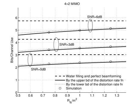
Figure 4: Information rate of finite size single rank beamforming codebooks

Although the approximation (37) is neither an upper bound nor a lower bound to the normalized information rate, it gives a good characterization under high feedback rate assumption. In fact, for a $4\times 2$ MIMO system with feedback rate $R_{\mathrm{fb}}=4$bits/channel use, the information rate calculated by (37) is very close to that evaluated by Monte Carlo simulation (see Fig. 4).

The constant $\mu$ is called as power efficiency factor. The effect of a finite size beamforming codebook can be viewed as decreasing the $P_{\mathrm{on}}$ in (6) to $\mu P_{\mathrm{on}}$ in (37). Thus for a given codebook size, the beamforming codebook should be designed to maximize the corresponding power efficiency factor $\mu$, or equivalently, to minimize the average squared chordal distance $\overline{d_{c}^{2}}$. However, it may be computational complex to design a codebook to minimize $\overline{d_{c}^{2}}$ directly. In [27], a criterion of maximizing the minimum chordal distance between any pair of beamforming matrices (max-min criterion) is proposed to achieve small $\overline{d_{c}^{2}}$. In this paper, we adopt the max-min criterion to design beamforming codebook for simplicity. Assuming that a beamforming codebook is well designed, the maximum $\mu$ achievable can be tightly upper and lower bounded as functions of the codebook size according to Theorem 5. Note that $K=2^{R_{\mathrm{fb}}}$ when $\bar{s}_{\infty}\geq\frac{1}{m}$ and $K=2^{R_{\mathrm{fb}}}-1\approx 2^{R_{\mathrm{fb}}}$ when $\bar{s}_{\infty}<\frac{1}{m}$. We have

$$1-\frac{\Gamma\left(\frac{1}{t}\right)}{st}\eta^{-\frac{1}{t}}2^{-\frac{R_{\mathrm{fb}}}{t}}\lesssim\mu_{\sup}\lesssim 1-\frac{t}{s\left(t+1\right)}\eta^{-\frac{1}{t}}2^{-\frac{R_{\mathrm{fb}}}{t}},$$ (38)

where $s$ is the rank of the single rank beamforming codebook, $t=s\left(L_{T}-s\right)$ and $\eta$ is given in (34). Comparing the imperfect beamforming case to the perfect beamforming case, the effective power loss $1-\mu_{\sup}$ decays exponentially with a rate proportional to $R_{\mathrm{fb}}/m^{2}$ (specifically, the exact rate of exponential decay is $\frac{m^{2}}{s\left(L_{T}-s\right)}\cdot\frac{R_{\mathrm{fb}}}{m^{2}}$). Thus for practical MIMO systems where $m$ is not large, a few bits may be enough to achieve a performance close to CSITR.

According to the above results, the information rate of a power on/off strategy with a well-designed single rank beamforming codebook can be well characterized. For a given $L_{T}\times L_{R}$ MIMO system with finite rate channel state feedback up to $R_{\mathrm{fb}}$ bits/channel use, $\mu_{\sup}$ can be estimated according to (38) for all $s$’s such that $1\leq s\leq L_{T}$. Substitute the bounds on $\mu_{\sup}$ into the information rate approximation (37) and then use the the asymptotic formulas in Section III-B1 for perfect beamforming case. The optimal number of on-beams $s$ and the corresponding information rate $\mathcal{I}$ can be calculated.

Fig. 4 gives the simulation results for a $4\times 2$ MIMO system. The performance curves are plotted as functions of $R_{\mathrm{fb}}/m^{2}$. The simulated information rate (circles) is compared to the information rate characterized by the lower bound (solid lines) and the upper bound (dotted lines) of $\overline{d_{c}^{2}}_{\inf}$. The simulation results show that the information rate characterized by the bounds (33) matches the actual performance almost perfectly. Note that the previous approximation proposed in [34, 33], which is based on asymptotic analysis and Gaussian approximation, overestimates the information rate (a correction of the result is in [35]). Our characterization is more accurate.

V Performance Comparison

While we have shown that power on/off strategy with a constant number of on-beams is near optimal for perfect beamforming in Section III, this section will show that a constant number of on-beams are near optimal when beamforming is imperfect as well.

To show the near optimality of a constant number of on-beams, the single rank beamforming codebooks are compared to multi-rank beamforming codebooks, which may contain beamforming matrices of different ranks. For a multi-rank beamforming codebook

$$\mathcal{B}=\left\{\mathbf{Q}_{i}\in\mathbb{C}^{L_{T}\times s}:\;\mathbf{Q}_{i}^{\dagger}\mathbf{Q}_{i}=\mathbf{I}_{s},\;0\leq s\leq L_{T},\;1\leq i\leq 2^{R_{\mathrm{fb}}}\right\},$$

define a single rank sub-code with rank $s$ as

$$\mathcal{B}_{s}\triangleq\left\{\mathbf{Q}_{i}:\;\mathbf{Q}_{i}\in\mathcal{B},\;\mathrm{rank}\left(\mathbf{Q}_{i}\right)=s\right\}$$

where $0\leq s\leq L_{T}$. The multi-rank beamforming codebook $\mathcal{B}$ can be viewed as a union of the single rank sub-codes $\mathcal{B}=\bigcup_{s=0}^{L_{T}}\mathcal{B}_{s}$. The corresponding power on/off strategy design problem is to find the optimal multi-rank beamforming codebook $\mathcal{B}$, feedback function $\varphi\left(\cdot\right)$ and constant $P_{\mathrm{on}}$ to maximize the information rate with a power constraint $\rho$, as stated in Problem 1.

It is difficult to solve the optimization problem for multi-rank beamforming codebooks. However, for a given multi-rank beamforming codebook $\mathcal{B}$ and a given $P_{\mathrm{on}}$, the following theorem gives the explicit form of the optimal feedback function, say $\tilde{\varphi}\left(\cdot\right)$, to avoid exhaustive search in all possible feedback functions. The intuition behind is same as the intuition which we learnt from Theorem 1: all the “good” beams and only the “good” beams should be turned on. The particular aspect of the following theorem is that “good” beams need to be reasonably defined.

Theorem 6

Consider the power on/off strategy with a given multi-rank beamforming codebook $\mathcal{B}=\bigcup_{s=0}^{L_{T}}\mathcal{B}_{s}$ and a given $P_{\mathrm{on}}$. For a given channel realization $\mathbf{H}$, define $\mathcal{I}_{s}\left(\mathbf{H}\right)$ as the largest mutual information achievable for a non-empty sub-code $\mathcal{B}_{s}$

$$\mathcal{I}_{s}\left(\mathbf{H}\right)=\underset{\mathbf{Q}_{i}\in\mathcal{B}_{s}}{\max}\;\ln\left|\mathbf{I}_{L_{R}}+P_{\mathrm{on}}\mathbf{HQ}_{i}\mathbf{Q}_{i}^{\dagger}\mathbf{\mathbf{H}}^{\dagger}\right|,$$

where $\mathcal{B}_{s}\neq\phi$, $0\leq s\leq L_{T}$ ($\mathcal{I}_{0}\left(\mathbf{H}\right)=0$). Denote the optimal feedback function as $\tilde{\varphi}\left(\cdot\right)$. Then

$$\tilde{\varphi}\left(\mathbf{H}\right)=\arg\;\underset{i:\;\mathbf{Q}_{i}\in\mathcal{B}_{\tilde{s}\left(\mathbf{H}\right)}}{\max}\;\ln\left|\mathbf{I}_{L_{R}}+P_{\mathrm{on}}\mathbf{H}\mathbf{Q}_{i}\mathbf{Q}_{i}^{\dagger}\mathbf{H}^{\dagger}\right|,$$

where

$$\tilde{s}\left(\mathbf{H}\right)\triangleq\max\left\{s:\;\mathcal{B}_{s}\neq\phi,\;\mathcal{I}_{s}\left(\mathbf{H}\right)-\mathcal{I}_{t}\left(\mathbf{H}\right)\geq(s-t)\kappa\;\textrm{for }\mathbf{all}\;t\;\textrm{s.t.}\;0\leq t<s,\;\mathcal{B}_{t}\neq\phi\right\}$$

and $\kappa$ is the appropriate threshold to satisfy the average power constraint

$$E_{\mathbf{H}}\left[\tilde{s}\left(\mathbf{H}\right)P_{\mathrm{on}}\right]=\rho.$$

Proof:

See Appendix -I. ∎

The following examples are direct applications of Theorem 6.

Example 1

Let $\mathcal{B}=\left\{\mathbf{I}_{L_{T}},\mathbf{Q}_{\phi}\right\}$ where $\mathbf{Q}_{\phi}$ is the artificial notion for the case that the transmitter is turned off. Then the optimal power on/off function is to turn on all transmit antennas if

$$\ln\left(\mathbf{I}_{L_{R}}+P_{\mathrm{on}}\mathbf{H}\mathbf{H}^{\dagger}\right)\geq\kappa L_{T}$$

and turn off the transmitter if

$$\ln\left(\mathbf{I}_{L_{R}}+P_{\mathrm{on}}\mathbf{H}\mathbf{H}^{\dagger}\right)<\kappa L_{T}$$

where $\kappa$ is an appropriate chosen threshold to satisfy

$$L_{T}P_{\mathrm{on}}\Pr\left\{\ln\left(\mathbf{I}+P_{\mathrm{on}}\mathbf{H}\mathbf{H}^{\dagger}\right)\geq\kappa L_{T}\right\}=\rho.$$

Example 2

Let $\left|\mathcal{B}\right|\rightarrow\infty$ and $\mathcal{B}$ is constructed so that the beamforming is asymptotically perfect. It is easy to verify that the optimal feedback function given by Theorem 6 is same as the one given in Theorem 1 for perfect beamforming case.

Although the optimal feedback function for a multi-rank beamforming codebook is given in Theorem 6, it is difficult to find the optimal multi-rank beamforming codebook $\mathcal{B}$, the optimal $P_{\mathrm{on}}$ and the corresponding information rate. In our simulation, we try different multi-rank codebooks and different $P_{\mathrm{on}}$’s and then choose the best one. Specifically, denote $K_{s}$ as the size of the sub-code $\mathcal{B}_{s}$, $K_{s}\triangleq\left|\mathcal{B}_{s}\right|$. We try all possible combinations of $\left[K_{0},K_{1},\cdots,K_{L_{T}}\right]$’s such that $K_{s}\in\mathbb{Z}^{+}\cup\left\{0\right\}$ and $\sum_{s=0}^{L_{T}}K_{s}\leq 2^{R_{\mathrm{fb}}}$. For each $\left[K_{0},K_{1},\cdots,K_{L_{T}}\right]$, we construct the sub-codes $\mathcal{B}_{s}$’s such that $\left|\mathcal{B}_{s}\right|=K_{s}$ for $s=0,1,\cdots,L_{T}$ according to the max-min criterion in [27]. The ultimate multi-rank beamforming codebook is given by $\mathcal{B}=\bigcup_{s=0}^{L_{T}}\mathcal{B}_{s}$. For every multi-rank codebook $\mathcal{B}$, we try different $P_{\mathrm{on}}$’s and search for the optimal one. The optimal multi-rank codebook $\mathcal{B}$ is chosen from the codebooks corresponding to all possible $\left[K_{0},K_{1},\cdots,K_{L_{T}}\right]$’s.

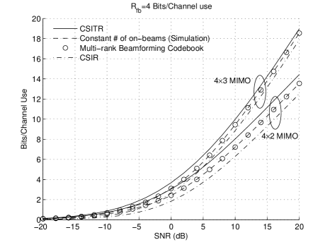
(a) Information rate

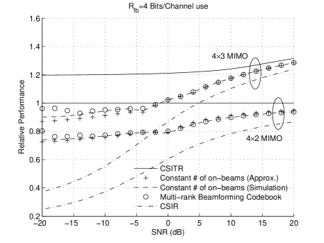
(b) Relative performance

Figure 5: Comparison of single rank beamforming codebooks and multi-rank beamforming codebooks

Fig. 5 shows the simulation results. Fig. 5(a) compares the information rates of single rank beamforming codebooks and multi-rank beamforming codebooks. Fig. 5(b) presents the relative performance, which is defined as the ratio of the considered information rate and the capacity of a $4\times 2$ MIMO system with perfect CSITR. We also present the information rate characterization by the upper bound of $\overline{d_{c}^{2}}_{\inf}$ (Section IV-B). Simulations show that single rank beamforming codebooks (dashed lines) achieve almost the same information rate of multi-rank beamforming codebooks (circles). The performance difference is noticeable in very low SNR regime. This is because the power on/off strategy with a single rank beamforming codebook is designed according to the asymptotic distribution of eigenvalues of $\frac{1}{m}\mathbf{H}\mathbf{H}^{\dagger}$ while the key parameters ($P_{\mathrm{on}}$ and $\kappa$) of power on/off strategy with multi-rank beamforming codebooks are numerically optimized according to the actual distribution of $\frac{1}{m}\mathbf{H}\mathbf{H}^{\dagger}$. According to the simulation results, power on/off strategy with constant number of on-beams provides a simple but near-optimal solution for finite rate channel state feedback.

VI Conclusions

This paper accurately characterizes the information rate of the power on/off strategy with finite rate channel state feedback. According to asymptotic analysis, the power on/off strategy with a constant number of on-beams is employed and studied. Simulations show that this strategy is near optimal for all SNR regimes. We derive asymptotic formulas for perfect beamforming case and introduce the power efficiency factor to quantify the effect of imperfect beamforming. By combining a formula for power efficiency factor and the asymptotic formulas for perfect beamforming, we characterize the corresponding information rate accurately for all SNR regimes.

An important point that is not mentioned in this paper is the complexity of selecting the feedback beamforming matrix in a codebook, which may involve exhaustive search. To avoid exhaustive search, beamforming codebooks with certain structure may be considered in future so that the matrix selection can be more efficient by employing the structure of the codebook.

-A Proof of Theorem 1

Let’s start with the single input single output (SISO) case. In SISO case, $\mathbf{H}$ is a scalar and $\frac{1}{m}\mathbf{H}^{\dagger}\mathbf{H}$ has only one eigenvalue, i.e., $\lambda=\left|\mathbf{H}\right|^{2}$. Denote the corresponding cumulative distribution function (CDF) as $F_{\Lambda}\left(\lambda\right)$. Define $\Omega$ as the set of $\lambda$ corresponding to the case that the transmitter is turned on. Then any deterministic power on/off strategy can be uniquely defined by $\Omega$. Thus the optimization problem is to choose an appropriate Lebesgue measurable set $\Omega\subset\mathbb{R}^{+}\cup\left\{0\right\}$ to maximize

$$\int_{\Omega}\log\left(1+P_{\mathrm{on}}\lambda\right)dF_{\Lambda}\left(\lambda\right)$$

with the power constraint

$$\int_{\Omega}dF_{\Lambda}\left(\lambda\right)=\rho/P_{\mathrm{on}}.$$

Since $F_{\Lambda}\left(\lambda\right)$ is continuous, there exists an $\Omega$ to satisfy the power constraint. The optimization problem is well defined.

Define $\Omega^{*}=\left\{\lambda:\;\lambda\geq\kappa\right\}$ such that $\int_{\Omega^{*}}dF_{\Lambda}\left(\lambda\right)=\rho/P_{on}$. For any Lebesgue measurable set $\Omega\subset\mathbb{R}^{+}\cup\left\{0\right\}$ such that $\int_{\Omega}dF_{\Lambda}\left(\lambda\right)=\rho/P_{\mathrm{on}}$,

$$\int_{\Omega^{*}}\log\left(1+P_{\mathrm{on}}\lambda\right)dF_{\Lambda}\left(\lambda\right)-\int_{\Omega}\log\left(1+P_{\mathrm{on}}\lambda\right)dF_{\Lambda}\left(\lambda\right)$$

$$\;=\int_{\Omega^{*}-\Omega}\log\left(1+P_{\mathrm{on}}\lambda\right)dF_{\Lambda}\left(\lambda\right)-\int_{\Omega-\Omega^{*}}\log\left(1+P_{\mathrm{on}}\lambda\right)dF_{\Lambda}\left(\lambda\right)$$

$$\;\overset{\left(a\right)}{\geq}\int_{\Omega^{*}-\Omega}\log\left(1+P_{\mathrm{on}}\kappa\right)dF_{\Lambda}\left(\lambda\right)-\int_{\Omega-\Omega^{*}}\log\left(1+P_{\mathrm{on}}\kappa\right)dF_{\Lambda}\left(\lambda\right)$$

$$\;=\log\left(1+P_{\mathrm{on}}\kappa\right)\left[\int_{\Omega^{*}-\Omega}dF_{\Lambda}\left(\lambda\right)-\int_{\Omega-\Omega^{*}}dF_{\Lambda}\left(\lambda\right)\right]$$

$$\;\overset{\left(b\right)}{=}0,$$

where

(a) follows from the facts that $\lambda\geq\kappa$ when $\lambda\in\Omega^{*}-\Omega$ and $\lambda<\kappa$ when $\lambda\in\Omega-\Omega^{*}$, and

(b) holds because $\int_{\Omega^{*}}dF_{\Lambda}\left(\lambda\right)=\int_{\Omega}dF_{\Lambda}\left(\lambda\right)$ implies $\int_{\Omega^{*}-\Omega}dF_{\Lambda}\left(\lambda\right)=\int_{\Omega-\Omega^{*}}dF_{\Lambda}\left(\lambda\right)$.

Therefore, $\Omega^{*}$ is the optimal set and the power on/off strategy defined by $\Omega^{*}$ is optimal.

The proof for MIMO case follows the same idea. For an $L_{T}\times L_{R}$ MIMO system, denote the vector of the ordered $L_{T}$ eigenvalues of $\mathbf{H}^{\dagger}\mathbf{H}$ as $\mathbf{\lambda}=\left[\lambda_{1},\cdots,\lambda_{L_{T}}\right]$ where $\lambda_{1}\geq\lambda_{2}\geq\cdots\geq\lambda_{L_{T}}\geq 0$ and the corresponding multivariate CDF as $F_{\mathbf{\Lambda}}\left(\mathbf{\lambda}\right)$. Define

$$\Omega_{k}=\left\{\mathbf{\lambda}:\;\mathrm{the\;eigen\;channel\;corresponding\;to\;}\lambda_{k}\;\mathrm{is\;on}\right\}$$

where $1\leq k\leq L_{T}$. Then any deterministic power on/off strategy can be uniquely defined by $\Omega_{k}$’s where $1\leq k\leq L_{T}$. The optimization problem is to choose Lebesgue measurable sets $\Omega_{k}\subset\left(\mathbb{R}^{+}\cup\left\{0\right\}\right)^{m}$, $k=1,2,\cdots,L_{T}$, to maximize

$$\sum_{k=1}^{L_{T}}\int_{\Omega_{k}}\ln\left(1+P_{\mathrm{on}}\lambda_{k}\right)dF_{\mathbf{\Lambda}}\left(\mathbf{\lambda}\right)$$

with the power constraint

$$\sum_{k=1}^{L_{T}}\int_{\Omega_{k}}dF_{\mathbf{\Lambda}}\left(\mathbf{\lambda}\right)=\rho/P_{\mathrm{on}}.$$

Since $F_{\mathbf{\Lambda}}\left(\mathbf{\lambda}\right)$ is continuous, there exist $\Omega_{k}$’s to satisfy the power constraint. The optimization problem is well defined.

Define $\Omega_{k}^{*}=\left\{\mathbf{\lambda}:\;\lambda_{1}\geq\cdots\geq\lambda_{k}\geq\kappa\right\}$’s where $\kappa$ is chosen to satisfy the power constraint. For any Lebesgue measurable sets $\Omega_{k}\subset\left(\mathbb{R}^{+}\cup\left\{0\right\}\right)^{m}$’s satisfying the power constraint,

$$\sum_{k=1}^{L_{T}}\int_{\Omega_{k}^{*}}\ln\left(1+P_{\mathrm{on}}\lambda_{k}\right)dF_{\mathbf{\Lambda}}\left(\mathbf{\lambda}\right)$$

$$\quad\quad-\sum_{k=1}^{L_{T}}\int_{\Omega_{k}}\ln\left(1+P_{\mathrm{on}}\lambda_{k}\right)dF_{\mathbf{\Lambda}}\left(\mathbf{\lambda}\right)$$

$$\geq\sum_{k=1}^{L_{T}}\int_{\Omega_{k}^{*}-\Omega_{k}}\ln\left(1+P_{\mathrm{on}}\kappa\right)dF_{\mathbf{\Lambda}}\left(\mathbf{\lambda}\right)$$

$$\quad\quad-\sum_{k=1}^{L_{T}}\int_{\Omega_{k}-\Omega_{k}^{*}}\ln\left(1+P_{\mathrm{on}}\kappa\right)dF_{\mathbf{\Lambda}}\left(\mathbf{\lambda}\right)$$

$$=0,$$

where the inequality follows the facts that $\lambda_{k}\geq\kappa$ when $\lambda_{k}\in\Omega_{k}^{*}-\Omega_{k}$ and $\lambda_{k}<\kappa$ when $\lambda_{k}\in\Omega_{k}-\Omega_{k}^{*}$, and the last line holds because of the power constraint. Therefore, the power on/off strategy defined by $\Omega_{k}^{*}$’s is optimal.

-B Proof of Theorem 3

The following lemma is needed to prove Theorem 3.

Lemma 2

For a continuous and differentiable function $h\left(x\right)$ defined on $\left(a,b\right)$, denote the first derivative as $h^{{}^{\prime}}\left(x\right)$. If $h\left(x\right)=0$ implies $h^{{}^{\prime}}\left(x\right)<0$, then $h\left(x\right)$ has at most one zero in its domain. Furthermore, denote $x_{0}$ as the unique zero if it exists, then $h\left(x\right)>0$ for all $x\in\left(a,x_{0}\right)$ and $h\left(x\right)<0$ for all $x\in\left(x_{0},b\right)$.

Proof:

$h\left(x\right)$ has at most one zero. Let $x_{0}$ be a zero of $h\left(x\right)$. Since $h^{{}^{\prime}}\left(x_{0}\right)<0$ according to the assumption, $\exists\epsilon>0$ such that $h\left(x_{0}+\epsilon\right)<0$, $h\left(x_{0}-\epsilon\right)>0$ and $h\left(x\right)\neq 0$ for all $x\in\left(x_{0}-\epsilon,x_{0}+\epsilon\right)$ but $x_{0}$. Now suppose that $x_{1}\in\left(a,b\right)$ be another zero of $h\left(x\right)$ adjacent to $x_{0}$. W.l.o.g, we assume that $x_{1}>x_{0}$. Then $x_{0}<x_{0}+\epsilon/2<x_{1}$. Note that $h\left(x\right)$ is continuous. $h\left(x\right)$ crosses the $x$ axis at $x_{1}$ from negative to positive as $x$ increases. Thus $h^{{}^{\prime}}\left(x_{1}\right)>0$. It contradicts with the assumption.

Assume that $x_{0}$ is the unique zero if it exists. Because of the continuity of $h\left(x\right)$, it is easy to verify that $h\left(x\right)>0$ for all $x\in\left(a,x_{0}\right)$ and $h\left(x\right)<0$ for all $x\in\left(x_{0},b\right)$. ∎

To prove Theorem 3, we discuss two cases. One case is that $\frac{d\bar{\mathcal{I}}_{\infty}}{da}$ has zeros in $\left(0,\pi\right)$ and the other case is that it has no zero in $\left(0,\pi\right)$.

Evaluate $\frac{d\bar{\mathcal{I}}_{\infty}}{da}$ for an $a\in\left(0,\pi\right)$. Denote

$$z\left(t\right) = \frac{\rho}{y\bar{s}_{\infty}}\left(1+y-2\sqrt{y}\cos\left(t\right)\right).$$ (39)

Then

$$\frac{d\bar{\mathcal{I}}_{\infty}}{da} = \frac{d}{da}\left[\int_{a}^{\pi}\ln\left(1+\frac{\rho}{y\bar{s}_{\infty}}\left(1+y-2\sqrt{y}\cos\left(t\right)\right)\right)f_{T}\left(t\right)dt\right]$$

$$= f_{T}\left(a\right)\left[1-\ln\left(1+z\left(a\right)\right)-\int_{a}^{\pi}\frac{1}{1+z\left(t\right)}\cdot\frac{f_{T}\left(t\right)}{\bar{s}_{\infty}}dt\right].$$

Define

$$J=1-\ln\left(1+z\left(a\right)\right)-\int_{a}^{\pi}\frac{1}{1+z\left(t\right)}\cdot\frac{f_{T}\left(t\right)}{\bar{s}_{\infty}}dt.$$ (40)

Because $f_{T}\left(a\right)>0$ for all $a\in\left(0,\pi\right)$, the sign of $\frac{d\bar{\mathcal{I}}_{\infty}}{da}$ is uniquely determined by $J$ when $a\in\left(0,\pi\right)$.

For the first case that $\frac{d\bar{\mathcal{I}}_{\infty}}{da}$ has zeros in $\left(0,\pi\right)$, we argue that $\frac{d\bar{\mathcal{I}}_{\infty}}{da}$ has a unique zero, say $a_{0}$, in $\left(0,\pi\right)$ and that $\bar{\mathcal{I}}_{\infty}$ is maximized at $a_{0}$. This can be accomplished by showing that $J=0$ implies $dJ/da<0$. Note that

$$\frac{dJ}{da} = -\frac{\frac{1}{\bar{s}_{\infty}}z\left(a\right)+\frac{\rho}{y\bar{s}_{\infty}}2\sqrt{y}\sin\left(a\right)}{1+z\left(a\right)}+\frac{f_{T}\left(a\right)}{\bar{s}_{\infty}}\cdot\frac{1}{1+z\left(a\right)}$$ (41)

$$-\frac{f_{T}\left(a\right)}{\bar{s}_{\infty}}\int_{a}^{\pi}\frac{1}{\left(1+z\left(t\right)\right)^{2}}\frac{f_{T}\left(t\right)}{\bar{s}_{\infty}}dt$$

$$= -\frac{f_{T}\left(a\right)}{\bar{s}_{\infty}}\left[\frac{z\left(a\right)-1}{z\left(a\right)+1}+\int_{a}^{\pi}\frac{1}{\left(1+z\left(t\right)\right)^{2}}\frac{f_{T}\left(t\right)}{\bar{s}_{\infty}}dt\right]$$

$$-\frac{\frac{\rho}{y\bar{s}_{\infty}}2\sqrt{y}\sin\left(a\right)}{1+z\left(a\right)}.$$

$J=0$ implies

$$1-\ln\left(1+z\left(a\right)\right) = \int_{a}^{\pi}\frac{1}{1+z\left(t\right)}\frac{f_{T}\left(t\right)}{\bar{s}_{\infty}}dt.$$

Then

$$\int_{a}^{\pi}\frac{1}{\left(1+z\left(t\right)\right)^{2}}\frac{f_{T}\left(t\right)}{\bar{s}_{\infty}}dt \geq \left(\int_{a}^{\pi}\frac{1}{1+z\left(t\right)}\frac{f_{T}\left(t\right)}{\bar{s}_{\infty}}dt\right)^{2}$$

$$= \left(1-\ln\left(1+z\left(a\right)\right)\right)^{2},$$

where the inequality follows the fact that

$$\int_{a}^{\pi}\left(\frac{1}{1+z\left(t\right)}-\int_{a}^{\pi}\frac{1}{1+z\left(t\right)}\frac{f_{T}\left(t\right)}{\bar{s}_{\infty}}dt\right)^{2}\frac{f_{T}\left(t\right)}{\bar{s}_{\infty}}dt \geq 0.$$

Thus,

$$\frac{z\left(a\right)-1}{z\left(a\right)+1}+\int_{a}^{\pi}\frac{1}{\left(1+z\left(t\right)\right)^{2}}\frac{f_{T}\left(t\right)}{\bar{s}_{\infty}}dt$$

$$\geq\frac{z\left(a\right)-1}{z\left(a\right)+1}+\left(1-\ln\left(1+z\left(a\right)\right)\right)^{2}$$

$$>0,$$

where the last inequality follows the facts that $z\left(a\right)>0$ for $a\in\left(0,\pi\right)$ and that $\frac{x-1}{x+1}+\left(1-\ln\left(1+x\right)\right)^{2}>0$ for $x>0$, which can be verified by evaluating the first and second derivatives. Therefore, $J=0$ implies that the first term of (41) is negative. It is also true that the last term of (41) is always negative for $a\in\left(0,\pi\right)$. We have shown that $J=0$ implies $dJ/da<0$. According to Lemma 2, $J$ has a unique zero in $\left(0,\pi\right)$, say $a_{0}$, and $J>0$ for $0<a<a_{0}$ and $J<0$ for $a_{0}<a<\pi$. Since the sign of $\frac{d\bar{\mathcal{I}}_{\infty}}{da}$ is determined by $J$, the same conclusion holds for $\frac{d\bar{\mathcal{I}}_{\infty}}{da}$. Therefore, $\bar{\mathcal{I}}_{\infty}$ has the unique maximum point $a_{0}$ in $\left(0,\pi\right)$. Furthermore, because of the continuity of $\bar{\mathcal{I}}_{\infty}$, $a_{0}$ is also the unique maximum point of $\bar{\mathcal{I}}_{\infty}$ in $\left[0,\pi\right]$.

For the second case that $\frac{d\bar{\mathcal{I}}_{\infty}}{da}$ has no zero in $\left(a,b\right)$, we show that $\bar{\mathcal{I}}_{\infty}$ is maximized at $a=0$. If $\frac{d\bar{\mathcal{I}}_{\infty}}{da}$ has no zero in $\left(a,b\right)$, $J$ has no zero in $\left(a,b\right)$. But as $a\rightarrow\pi$, it can be verified that $z\left(a\right)\rightarrow+\infty$, $\ln\left(1+z\left(a\right)\right)\rightarrow+\infty$ and $J\rightarrow-\infty$. Then $J<0$ for $a\in\left(0,\pi\right)$ because of continuity. Therefore, $\frac{d\bar{\mathcal{I}}_{\infty}}{da}<0$ for all $a\in\left(0,\pi\right)$ and $\bar{\mathcal{I}}_{\infty}$ is maximized at $a=0$.

-C Proof of Corollary 2

The proof follows the same idea in the proof of Theorem 3 (see Appendix -B). Let $J$ be defined in (40). Then the optimal $a$ to maximize $\bar{\mathcal{I}}_{\infty}$, say $a_{0}$, should be either the unique zero of $J$ if it exists, or $0$ if $J$ has no zero in $\left(0,\pi\right)$. We first prove that $J=0$ implies $\frac{dJ}{d\rho}<0$ for a given $a\in\left(0,\pi\right)$ and $\rho>0$. Then we show that $a_{0}$ is a non-decreasing function of $\rho$.

For a given $a\in\left(0,\pi\right)$ and $\rho>0$, we prove that $J=0$ implies $\frac{dJ}{d\rho}<0$ as follows. Let $z\left(t\right)$ be defined in (39). Note that $z\left(t\right)$ is a function of $\rho$. Evaluation of $\frac{dJ}{d\rho}$ gives

$$\frac{dJ}{d\rho} = -\frac{1}{\rho}\left[\frac{z\left(a\right)}{1+z\left(a\right)}-\int_{a}^{\pi}\frac{z\left(t\right)}{\left(1+z\left(t\right)\right)^{2}}\frac{f_{T}\left(t\right)}{\bar{s}_{\infty}}dt\right]$$ (42)

$$= -\frac{1}{\rho}\left[\frac{z\left(a\right)}{1+z\left(a\right)}-\int_{a}^{\pi}\frac{z\left(t\right)}{1+z\left(t\right)}\frac{f_{T}\left(t\right)}{\bar{s}_{\infty}}dt\right.$$

$$\left.+\int_{a}^{\pi}\frac{z^{2}\left(t\right)}{\left(1+z\left(t\right)\right)^{2}}\frac{f_{T}\left(t\right)}{\bar{s}_{\infty}}dt\right].$$

$J=0$ implies

$$\ln\left(1+z\left(a\right)\right)=\int_{a}^{\pi}\frac{z\left(t\right)}{1+z\left(t\right)}\frac{f_{T}\left(t\right)}{\bar{s}_{\infty}}dt<1,$$ (43)

where the inequality follows the fact that $\frac{z\left(t\right)}{1+z\left(t\right)}<1$. Then we have $z\left(a\right)<e-1$. Furthermore,

$$\int_{a}^{\pi}\frac{z^{2}\left(t\right)}{\left(1+z\left(t\right)\right)^{2}}\frac{f_{T}\left(t\right)}{\bar{s}_{\infty}}dt \geq \frac{z^{2}\left(a\right)}{\left(1+z\left(a\right)\right)^{2}},$$ (44)

where the inequality follows from $\frac{z\left(t\right)}{1+z\left(t\right)}\geq\frac{z\left(a\right)}{1+z\left(a\right)}$ for all $t\in\left(a,\pi\right)$. Note that the function $\frac{x}{1+x}-\ln\left(1+x\right)+\left(\frac{x}{1+x}\right)^{2}>0$ for $0<x<e-1$, which can be verified by checking its first and second derivative. Substituting (43) and (44) into (42), we have shown that $J=0$ implies $\frac{dJ}{d\rho}<0$ for $a\in\left(0,\pi\right)$.

Now let $a_{0}$ maximize $\bar{\mathcal{I}}_{\infty}$ for an SNR $\rho_{0}>0$, let $a_{1}$ maximize $\bar{\mathcal{I}}_{\infty}$ for an SNR $\rho_{1}>0$ and $\rho_{0}<\rho_{1}$. In the following, we prove that $a_{1}\leq a_{0}$ by studying two cases: one is that $a_{0}>0$ and the other is that $a_{0}=0$.

For the first case that $a_{0}>0$, we have $J\left|{}_{a_{0},\rho_{0}}\right.=0$ by Theorem 3. Since $J=0$ implies $\frac{dJ}{d\rho}<0$ for $a=a_{0}$, $J\left|{}_{a_{0},\rho_{1}}\right.<0$ by Lemma 2 in Appendix -B. But $a_{1}$ maximizes $\bar{\mathcal{I}}_{\infty}$ at $\rho_{1}$. Then either $a_{1}=0$, or $a_{1}>0$ and $J\left|{}_{a_{1},\rho_{1}}\right.=0$ again by Theorem 3. If $a_{1}=0$, $a_{1}<a_{0}$. If $a_{1}>0$, then $\frac{dJ}{da}\left|{}_{0<a<a_{1},\rho_{1}}\right.>0$ and $\frac{dJ}{da}\left|{}_{a_{1}<a<\pi,\rho_{1}}\right.<0$ according to the proof in Appendix -B. Since we have shown $J\left|{}_{a_{0},\rho_{1}}\right.<0$, $a_{1}<a_{0}$. Thus $a_{1}<a_{0}$ if $a_{0}>0$.

On the other hand, $a_{0}=0$ implies $a_{1}=a_{0}=0$. Suppose that $a_{1}>a_{0}$, then $a_{1}\in\left(0,\pi\right)$, $J\left|{}_{a_{1},\rho_{1}}\right.=0$ and $J\left|{}_{a_{1},\rho_{0}}\right.>0$. Because $J\left|{}_{\pi,\rho_{0}}\right.\rightarrow-\infty$, $\exists a^{\prime}\in\left(a_{1},\pi\right)$ such that $J\left|{}_{a^{\prime},\rho_{0}}\right.=0$. According to Theorem 3, $a^{\prime}$ maximizes $\bar{\mathcal{I}}_{\infty}$ for $\rho_{0}$. It contradicts with the assumption that $a_{0}=0$ maximizes $\bar{\mathcal{I}}_{\infty}$ for $\rho_{0}$. Therefore $0\leq a_{1}\leq a_{0}=0$ and thus $a_{1}=a_{0}=0$.

-D Calculation of $\bar{s}_{\infty}$

Write the formula for $\bar{s}_{\infty}$ in (13) in another form. Recall the definition of $f_{T}\left(t\right)$ in (12). It is easy to see that $f_{T}\left(t\right)=f_{T}\left(-t\right)$. In order to use the symmetry, we define the integral range

$$I_{R} = \left[-\pi,-a\right]\cup\left[a,\pi\right].$$ (45)

Then the normalized number of on-beams $\bar{s}_{\infty}$ is given by

$$\bar{s}_{\infty}=\frac{1}{2}\int_{I_{R}}f_{T}\left(t\right)dt.$$

When $y<1$,

$$\bar{s}_{\infty} = \frac{1}{2}\int_{I_{R}}\frac{1}{2\pi}\cdot\frac{2-e^{2it}-e^{-2it}}{1+r^{2}-2r\cos\left(t\right)}dt$$

$$= \frac{1}{4\pi\left(1-r^{2}\right)}\int_{I_{R}}\left(\frac{1}{1-re^{it}}+\frac{1}{1-re^{-it}}-1\right)\left(2-e^{2it}-e^{-2it}\right)dt,$$

where $r=\sqrt{y}$. Because of the symmetry of the integral range and the integrand, we have

$$\int_{I_{R}}\frac{1}{1-re^{it}}\left(2-e^{2it}-e^{-2it}\right)dt=\int_{I_{R}}\frac{1}{1-re^{-it}}\left(2-e^{2it}-e^{-2it}\right)dt.$$

Then

$$\bar{s}_{\infty} = \frac{1}{4\pi\left(1-r^{2}\right)}\int_{I_{R}}\left(\frac{2}{1-re^{it}}-1\right)\left(2-e^{2it}-e^{-2it}\right)dt$$

$$= \frac{1}{4\pi\left(1-r^{2}\right)}\int_{I_{R}}\left[-2\left(\frac{1}{r}-r\right)^{2}\frac{re^{it}}{1-re^{it}}\right.$$

$$\left.+e^{2it}+\frac{2}{r}e^{it}+2-2r^{2}-2re^{-it}-e^{-2it}\right]dt.$$

Note that

$$\int_{I_{R}}\frac{re^{it}}{1-re^{it}}dt=i\int_{I_{R}}d\ln\left(1-re^{it}\right)=i\ln\left(\frac{1-re^{-ia}}{1-re^{ia}}\right)=-2\theta_{r},$$ (46)

where

$$\theta_{r}=\tan^{-1}\left(\frac{r\sin\left(a\right)}{1-r\cos\left(a\right)}\right).$$

Then

$$\bar{s}_{\infty}=\frac{1}{\pi}\left(\left(\pi-a\right)-\frac{1}{r}\sin\left(a\right)+\frac{1-r^{2}}{r^{2}}\theta_{r}\right).$$

When $y=1$, it is easy to see that

$$\bar{s}_{\infty}=\frac{1}{2\pi}\int_{I_{R}}\left(1+\cos\left(t\right)\right)dt=\frac{1}{\pi}\left(\pi-a-\sin\left(a\right)\right)$$

-E Calculation of $\bar{\mathcal{I}}_{\infty}$

The normalized capacity is given by

$$\bar{\mathcal{I}}_{\infty}=\frac{1}{2}\int_{I_{R}}\ln\left(1+\frac{\rho}{\bar{s}_{\infty}y}\left(1+y-2\sqrt{y}\cos\left(t\right)\right)\right)f_{T}\left(t\right)dt$$

where $f_{T}\left(t\right)$ is given in (12), the integral range $I_{R}$ is defined in (45) and $\bar{s}_{\infty}$ can be calculated according to the Proposition 1.

Define

$$\alpha = \frac{\bar{s}_{\infty}y}{\rho},$$ (47)

then

$$\ln\left(1+\frac{\rho}{\bar{s}_{\infty}y}\left(1+y-2\sqrt{y}\cos\left(t\right)\right)\right)$$

$$=\ln\left(1+r^{2}+\alpha-2r\cos\left(t\right)\right)-\ln\left(\alpha\right),$$

where $r=\sqrt{y}$. Also define

$$w=\frac{1}{2}\left(1+y+\alpha+\sqrt{\left(1+y+\alpha\right)^{2}-4y}\right)$$ (48)

and

$$u=\frac{1}{2\sqrt{y}}\left(1+y+\alpha-\sqrt{\left(1+y+\alpha\right)^{2}-4y}\right),$$ (49)

then it is easy to verify that $u<1$ and

$$\ln\left(1+r^{2}+\alpha-2r\cos\left(t\right)\right)$$

$$=\ln\left(w\right)+\ln\left(1+u^{2}-2u\cos\left(t\right)\right).$$

Therefore,

$$\ln\left(1+\frac{\rho}{\bar{s}_{\infty}y}\left(1+y-2\sqrt{y}\cos\left(t\right)\right)\right)$$

$$=\ln\left(w\right)-\ln\left(\alpha\right)+\ln\left(1+u^{2}-2u\cos\left(t\right)\right),$$

and

$$\bar{\mathcal{I}}_{\infty} = \left(\ln\left(w\right)-\ln\left(\alpha\right)\right)\bar{s}_{\infty}$$

$$+\frac{1}{2}\int_{I_{R}}\ln\left(1+u^{2}-2u\cos\left(t\right)\right)f_{T}\left(t\right)dt.$$

Define

$$I_{0}=\frac{1}{2}\int_{I_{R}}\ln\left(1+u^{2}-2u\cos\left(t\right)\right)f_{T}\left(t\right)dt.$$

Then

$$\bar{\mathcal{I}}=\left(\ln\left(w\right)-\ln\left(\alpha\right)\right)\bar{s}+I_{0}.$$

Note that

$$\ln\left(1+u^{2}-2u\cos\left(t\right)\right)=\ln\left(1-ue^{it}\right)+\ln\left(1-ue^{-it}\right)$$

and

$$\int_{I_{R}}\ln\left(1-ue^{it}\right)f_{T}\left(t\right)dt = \int_{I_{R}}\ln\left(1-ue^{-it}\right)f_{T}\left(t\right)dt.$$

Then

$$I_{0}=\int_{I_{R}}\ln\left(1-ue^{it}\right)f_{T}\left(t\right)dt.$$

Calculate $I_{0}$ for the case $y<1$ and the case $y=1$ respectively.

When $y<1$,

$$I_{0} = \int_{I_{R}}\ln\left(1-ue^{it}\right)\cdot\frac{1}{2\pi}\cdot\frac{2-e^{2it}-e^{-2it}}{1+r^{2}-2r\cos\left(t\right)}dt$$

$$= \frac{1}{2\pi\left(1-r^{2}\right)}\int_{I_{R}}\ln\left(1-ue^{it}\right)\left(\frac{1}{1-re^{it}}+\frac{1}{1-re^{-it}}-1\right)\left(2-e^{2it}-e^{-2it}\right)dt.$$

It is easy to verify that

$$\frac{e^{2it}-2+e^{-2it}}{1-re^{it}}=\left(\frac{1}{r}-r\right)^{2}\frac{re^{it}}{1-re^{it}}+\left(-\frac{1}{r}e^{it}-2+r^{2}+re^{-it}+e^{-2it}\right)$$ (50)

and

$$\frac{e^{2it}-2+e^{-2it}}{1-re^{-it}}=\left(\frac{1}{r}-r\right)^{2}\frac{1}{1-re^{it}}+\left(e^{2it}+re^{it}-\frac{1}{r^{2}}-\frac{1}{r}e^{-it}\right).$$ (51)

Then

$$\left(\frac{1}{1-re^{it}}+\frac{1}{1-re^{-it}}-1\right)\left(e^{2it}-2+e^{-2it}\right)$$

$$=\left(r-\frac{1}{r}\right)\left[e^{it}+\frac{1}{r}+r+e^{-it}+\left(r-\frac{1}{r}\right)\cdot\left(\frac{re^{it}}{1-re^{it}}+\frac{1}{1-re^{-it}}\right)\right].$$

Define

$$I_{1} = \int_{I_{R}}\ln\left(1-ue^{it}\right)dt$$ (52)

$$I_{2} = \int_{I_{R}}\ln\left(1-ue^{it}\right)\left(e^{it}+e^{-it}\right)dt$$ (53)

$$I_{3} = \int_{I_{R}}\ln\left(1-ue^{it}\right)\left(\frac{re^{it}}{1-re^{it}}+\frac{1}{1-re^{-it}}\right)dt,$$

Then

$$I_{0}=\frac{1}{2\pi r}\left[\left(\frac{1}{r}+r\right)I_{1}+I_{2}+\left(r-\frac{1}{r}\right)I_{3}\right].$$

Calculate $I_{1}$, $I_{2}$ and $I_{3}$ respectively. Because $\left|u\right|<1$,

$$\ln\left(1-ue^{it}\right)=-\sum_{k=1}^{\infty}\frac{u^{k}e^{ikt}}{k}.$$

Therefore,

$$I_{1} = -\int_{I_{R}}\sum_{k=1}^{\infty}\frac{u^{k}e^{ikt}}{k}dt$$

$$= -\sum_{k=1}^{\infty}\frac{u^{k}}{ik^{2}}\int_{I_{R}}de^{ikt}$$

$$= i\sum_{k=1}^{\infty}\frac{u^{k}e^{-ika}}{k^{2}}-i\sum_{k=1}^{\infty}\frac{u^{k}e^{ika}}{k^{2}}.$$

Define

$$\mathrm{Li}_{2}\left(x\right)=\sum_{n=1}^{\infty}\frac{x^{n}}{n^{2}},\;\;\mathrm{for}\>\left|x\right|\leq 1,$$

which is usually called dilogarithm function [42]. Then

$$I_{1} = i\left[\mathrm{Li}_{2}\left(ue^{-ia}\right)-\mathrm{Li}_{2}\left(ue^{ia}\right)\right].$$ (54)

To evaluate $I_{2}$, note that

$$\int_{I_{R}}\ln\left(1-ue^{it}\right)e^{it}dt = \int_{I_{R}}\frac{ue^{2it}}{1-ue^{it}}dt+\frac{1}{i}\ln\left(1-ue^{it}\right)e^{it}\left|{}_{a}^{\pi}\right.$$

$$+\frac{1}{i}\ln\left(1-ue^{it}\right)e^{it}\left|{}_{-\pi}^{-a}\right.$$

and

$$\int_{I_{R}}\ln\left(1-ue^{it}\right)e^{-it}dt = \int_{I_{R}}\frac{u}{1-ue^{it}}dt+\frac{1}{-i}\ln\left(1-ue^{it}\right)e^{-it}\left|{}_{a}^{\pi}\right.$$

$$+\frac{1}{-i}\ln\left(1-ue^{it}\right)e^{-it}\left|{}_{-\pi}^{-a}\right..$$

Then

$$I_{2} = -2\sin\left(a\right)\ln\left(1+u^{2}-2u\cos\left(a\right)\right)+u\int_{I_{R}}\frac{e^{2it}-1}{1-ue^{it}}dt.$$

Note that

$$u\frac{e^{2it}-1}{1-ue^{it}} = -e^{it}-u+\left(\frac{1}{u}-u\right)\frac{ue^{it}}{1-ue^{it}}$$

and

$$\int_{I_{R}}\frac{ue^{it}}{1-ue^{it}}dt=-2\theta_{u},$$

where

$$\theta_{u}=\tan^{-1}\left(\frac{u\sin\left(a\right)}{1-u\cos\left(a\right)}\right)$$

by similar analysis that we did in (46). Then

$$I_{2} = 2\left[-\sin\left(a\right)\ln\left(1+u^{2}-2u\cos\left(a\right)\right)\right.$$ (55)

$$\left.+\sin\left(a\right)-u\left(\pi-a\right)-\left(\frac{1}{u}-u\right)\theta_{u}\right].$$

To evaluate $I_{3}$, note that

$$\ln\left(1-ue^{it}\right) = -\sum_{k=1}^{\infty}\frac{\left(ue^{it}\right)^{k}}{k}$$

and

$$\frac{1}{1-re^{it}}+\frac{1}{1-re^{-it}}-1 = \sum_{l=-\infty}^{\infty}r^{\left|l\right|}e^{ilt}$$

because $\left|u\right|<1$ and $\left|r\right|<1$. Thus

$$-I_{3}=\int_{I_{R}}\sum_{k=1}^{\infty}\frac{\left(ue^{it}\right)^{k}}{k}\left(\sum_{l=-\infty}^{\infty}r^{\left|l\right|}e^{ilt}\right)dt.$$

Change the order of the double summation. Then

$$-I_{3} = \int_{I_{R}}\sum_{l=0}^{\infty}\left(\sum_{k=1}^{\infty}\frac{\left(ue^{it}\right)^{k}}{k}\left(re^{-it}\right)^{k+l}\right)dt$$

$$+\int_{I_{R}}\sum_{l=1}^{\infty}\left(\sum_{k=1}^{l-1}\frac{\left(ue^{it}\right)^{k}}{k}\left(re^{it}\right)^{l-k}+\sum_{k=l}^{\infty}\frac{\left(ue^{it}\right)^{k}}{k}\left(re^{-it}\right)^{k-l}\right)dt$$

$$= \int_{I_{R}}\sum_{l=0}^{\infty}r^{l}e^{-ilt}\left(\sum_{k=1}^{\infty}\frac{\left(ur\right)^{k}}{k}\right)dt$$

$$+\int_{I_{R}}\sum_{l=1}^{\infty}e^{ilt}\left(r^{l}\sum_{k=1}^{l-1}\frac{\left(\frac{u}{r}\right)^{k}}{k}+r^{-l}\sum_{k=l}^{\infty}\frac{\left(ur\right)^{k}}{k}\right)dt.$$

Define

$$I_{4} = \int_{I_{R}}\sum_{l=0}^{\infty}r^{l}e^{-ilt}\left(\sum_{k=1}^{\infty}\frac{\left(ur\right)^{k}}{k}\right)dt$$

and

$$I_{5} = \int_{I_{R}}\sum_{l=1}^{\infty}e^{ilt}\left(r^{l}\sum_{k=1}^{l-1}\frac{\left(\frac{u}{r}\right)^{k}}{k}+r^{-l}\sum_{k=l}^{\infty}\frac{\left(ur\right)^{k}}{k}\right)dt.$$

Noting that $0<r<1$ and $0<ur<1$, $I_{4}$ is well defined and

$$I_{4} = \sum_{k=1}^{\infty}\frac{\left(ur\right)^{k}}{k}\left(i\sum_{l=1}^{\infty}\frac{r^{l}}{l}e^{-ilt}+t\right)\left|\begin{array}[]{c}^{\pi}\\ _{a}\end{array}\right.$$

$$+\sum_{k=1}^{\infty}\frac{\left(ur\right)^{k}}{k}\left(i\sum_{l=1}^{\infty}\frac{r^{l}}{l}e^{-ilt}+t\right)\left|\begin{array}[]{c}^{-a}\\ _{-\pi}\end{array}\right.$$

$$= -\ln\left(1-ur\right)\left(t-i\ln\left(1-re^{-it}\right)\right)\left|{}_{a}^{\pi}\right.$$

$$-\ln\left(1-ur\right)\left(t-i\ln\left(1-re^{-it}\right)\right)\left|{}_{-\pi}^{-a}\right.$$

$$= -2\ln\left(1-ur\right)\left(\pi-a-\theta_{r}\right),$$ (62)

where $\theta_{r}$ is obtained according to the similar analysis in (46). To evaluate $I_{5}$, we substitute the definition of $u$ into $\frac{u}{r}$. It is easy to verify that

$$\frac{u}{r} = \frac{1}{2r^{2}}\left(1+r^{2}+\alpha-\sqrt{\left(1+r^{2}+\alpha\right)^{2}-4r^{2}}\right)$$

$$< \frac{1}{2r^{2}}\left(1+r^{2}+\alpha-\sqrt{\left(1-r^{2}+\alpha\right)^{2}}\right)$$

$$= 1$$

and

$$\left|I_{5}\right| \leq \int_{I_{R}}\sum_{l=1}^{\infty}r^{l}\left(\sum_{k=1}^{l-1}\frac{\left(ur\right)^{k}}{k}+r^{-2l}\sum_{k=l}^{\infty}\frac{\left(\frac{u}{r}\right)^{k}}{k}\right)dt$$

$$\leq \int_{I_{R}}\sum_{l=1}^{\infty}r^{l}\left(\sum_{k=1}^{l-1}\frac{\left(\frac{u}{r}\right)^{k}}{k}+\sum_{k=l}^{\infty}\frac{\left(\frac{u}{r}\right)^{k}}{k}\right)dt$$

$$= -\int_{I_{R}}\frac{r}{1-r}\ln\left(1-\frac{u}{r}\right)dt.$$

Therefore, $I_{5}$ is well defined. Further, define a special function in the form of series as

$$\mathrm{Sr}_{1}\left(u,r,t\right)=\sum_{l=1}^{\infty}\frac{r^{l}e^{ilt}}{l}\left(\sum_{k=1}^{l-1}\frac{\left(\frac{u}{r}\right)^{k}}{k}+r^{-2l}\sum_{k=l}^{\infty}\frac{r^{2k}\left(\frac{u}{r}\right)^{k}}{k}\right).$$

Then

$$I_{5} = \frac{1}{i}\mathrm{Sr}_{1}\left(u,r,t\right)\left|{}_{a}^{\pi}\right.+\frac{1}{i}\mathrm{Sr}_{1}\left(u,r,t\right)\left|{}_{-\pi}^{-a}\right.$$ (63)

$$= i\mathrm{Sr}_{1}\left(u,r,a\right)-i\mathrm{Sr}_{1}\left(u,r,-a\right).$$

In conclusion, when $y<1$,

$$\bar{\mathcal{I}}_{\infty} = \left[\ln\left(w\right)-\ln\left(\alpha\right)\right]\bar{s}_{\infty}+\frac{1}{2\pi r}\left(\frac{1+r^{2}}{r}I_{1}+I_{2}-\frac{1-r^{2}}{r}I_{3}\right)$$

$$= \left[\ln\left(w\right)-\ln\left(\alpha\right)\right]\bar{s}_{\infty}$$

$$+\frac{1+r^{2}}{2\pi r^{2}}I_{1}+\frac{1}{2\pi r}I_{2}+\frac{1-r^{2}}{2\pi r^{2}}I_{4}+\frac{1-r^{2}}{2\pi r^{2}}I_{5}$$

where $I_{1}$, $I_{2}$, $I_{4}$ and $I_{5}$ can be calculated according to (54-63).

When $y=1$, the calculation can be highly simplified. Substitute $f_{T}\left(t\right)$ into $I_{0}$, then

$$I_{0} = \frac{1}{2\pi}\int_{I_{R}}\ln\left(1-ue^{it}\right)\left(e^{it}+2+e^{-it}\right)dt$$

$$= \frac{1}{\pi}I_{1}+\frac{1}{2\pi}I_{2},$$

where $I_{1}$ and $I_{2}$ are defined in (52) and (53) respectively. Thus

$$\bar{\mathcal{I}}_{\infty} = \left[\ln\left(w\right)-\ln\left(\alpha\right)\right]\bar{s}_{\infty}+\frac{1}{\pi}I_{1}+\frac{1}{2\pi}I_{2},$$

where $I_{1}$and $I_{2}$ can be calculated by (54) and (55) respectively.

-F Calculation of $d\bar{\mathcal{I}}_{\infty}/da$

Define $I_{R}$, $\alpha$, $w$ and $u$ as (45), (47), (48) and (49). It is easy to see that

$$\frac{d\alpha}{da} = -\frac{y}{\rho}f_{T}\left(a\right).$$ (64)

According to the formula for the normalized information rate $\bar{\mathcal{I}}_{\infty}$ in (14),

$$\frac{d\bar{\mathcal{I}}_{\infty}}{da} = -\ln\left(1+\frac{1}{\alpha}\left(1+y-2\sqrt{y}\cos\left(a\right)\right)\right)f_{T}\left(a\right)$$

$$+\frac{1}{2}\int_{I_{R}}\frac{-\frac{1}{\alpha^{2}}\cdot\frac{d\alpha}{da}\cdot\left(1+y-2\sqrt{y}\cos\left(t\right)\right)}{1+\frac{1}{\alpha}\left(1+y-2\sqrt{y}\cos\left(t\right)\right)}f_{T}\left(t\right)dt.$$

By (64),

$$\frac{1}{2}\int_{I_{R}}\frac{-\frac{1}{\alpha^{2}}\cdot\frac{d\alpha}{da}\cdot\left(1+y-2\sqrt{y}\cos\left(t\right)\right)}{1+\frac{1}{\alpha}\left(1+y-2\sqrt{y}\cos\left(t\right)\right)}f_{T}\left(t\right)dt$$

$$=\frac{y}{2\rho\alpha}f_{T}\left(a\right)\int_{I_{R}}\frac{1+y-2\sqrt{y}\cos\left(t\right)}{1+y+\alpha-2\sqrt{y}\cos\left(t\right)}f_{T}\left(t\right)dt$$

$$=f_{T}\left(a\right)\left(1-\frac{y}{2\rho}\int_{I_{R}}\frac{1}{1+y+\alpha-2\sqrt{y}\cos\left(t\right)}f_{T}\left(t\right)dt\right).$$

Define

$$I^{d} =\frac{1}{2} \int_{I_{R}}\frac{1}{1+y+\alpha-2\sqrt{y}\cos\left(t\right)}f_{T}\left(t\right)dt.$$

then

$$\frac{d\bar{\mathcal{I}}_{\infty}}{da} = f_{T}\left(a\right)\left[1-\ln\left(1+\frac{1}{\alpha}\left(1+y-2\sqrt{y}\cos\left(a\right)\right)\right)-\frac{y}{\rho}I^{d}\right].$$ (65)

Consider the calculation of $I^{d}$. Since $w\left(1+u^{2}-2u\cos\left(t\right)\right)=1+y+\alpha-2\sqrt{y}\cos\left(t\right)$,

$$I^{d} = \frac{1}{2w}\int_{I_{R}}\frac{1}{1+u^{2}-2u\cos\left(t\right)}f_{T}\left(t\right)dt$$

$$= \frac{1}{2w\left(1-u^{2}\right)}\int_{I_{R}}\left(\frac{1}{1-ue^{it}}+\frac{1}{1-ue^{-it}}-1\right)f_{T}\left(t\right)dt.$$

According to the symmetry of $I_{R}$ and $f_{T}\left(t\right)$,

$$\int_{I_{R}}\frac{1}{1-ue^{it}}f_{T}\left(t\right)dt = \int_{I_{R}}\frac{1}{1-ue^{-it}}f_{T}\left(t\right)dt.$$

Then

$$I^{d} = \frac{1}{2w\left(1-u^{2}\right)}\int_{I_{R}}\left(\frac{2}{1-ue^{it}}-1\right)f_{T}\left(t\right)dt.$$

Calculate $I^{d}$ for the case $y<1$ and the case $y=1$ respectively.

When $y<1$,

$$I^{d} = \frac{1}{4\pi w\left(1-u^{2}\right)}\int_{I_{R}}\left(\frac{2}{1-ue^{it}}-1\right)\frac{2-e^{2it}-e^{-2it}}{1+r^{2}-2r\cos\left(t\right)}dt$$

$$= \frac{1}{4\pi w\left(1-u^{2}\right)\left(1-r^{2}\right)}\int_{I_{R}}\left[\left(\frac{2}{1-ue^{it}}-1\right)\right.$$

$$\left.\left(\frac{1}{1-re^{it}}+\frac{1}{1-re^{-it}}-1\right)\left(2-e^{2it}-e^{-2it}\right)\right]dt.$$

Expand the integrand. Since

$$\frac{1}{1-ue^{it}}\cdot\frac{1}{1-re^{it}}$$

$$=-\frac{u}{r-u}\frac{1}{1-ue^{it}}+\frac{r}{r-u}\frac{1}{1-re^{it}}$$

and

$$\frac{1}{1-ue^{it}}\cdot\frac{1}{1-re^{it}}$$

$$=\frac{1}{1-ur}\frac{1}{1-ue^{it}}-\frac{1}{1-ur}\frac{1}{1-\frac{1}{r}e^{it}},$$

$I^{d}$ can be split into four parts

$$I^{d} = \frac{1}{4\pi w\left(1-u^{2}\right)\left(1-r^{2}\right)}\left(I_{6}+I_{7}+I_{8}+I_{9}\right),$$

where

$$I_{6} = 2\left(\frac{1}{1-ur}-\frac{u}{r-u}-1\right)\int_{I_{R}}\frac{2-e^{2it}-e^{-2it}}{1-ue^{it}}dt,$$

$$I_{7} = 2\left(\frac{r}{r-u}-1\right)\int_{I_{R}}\frac{2-e^{2it}-e^{-2it}}{1-re^{it}}dt,$$

$$I_{8} = -\frac{2}{1-ur}\int_{I_{R}}\frac{2-e^{2it}-e^{-2it}}{1-\frac{1}{r}e^{it}}dt$$

and

$$I_{9} = \int_{I_{R}}\left(2-e^{2it}-e^{-2it}\right)dt.$$

$I_{9}$ can be easily calculated,

$$I_{9}=4\left(\pi-a\right).$$

To evaluate $I_{6}$, $I_{7}$ and $I_{8}$, expand the integrands like what has been done in (50). Note that

$$\int_{I_{R}}\frac{\frac{1}{r}e^{it}}{1-\frac{1}{r}e^{it}}dt = \int_{I_{R}}\left(-1-\frac{re^{-it}}{1-re^{-it}}\right)dt$$

$$= -\int_{I_{R}}\left(1+\frac{re^{it}}{1-re^{it}}\right)dt,$$

$$\int_{I_{R}}\frac{ue^{it}}{1-ue^{it}}dt=-2\theta_{u}$$

and

$$\int_{I_{R}}\frac{re^{it}}{1-re^{it}}dt=-2\theta_{r},$$

where

$$\theta_{u}=\tan^{-1}\left(\frac{u\sin\left(a\right)}{1-u\cos\left(a\right)}\right)$$

and

$$\theta_{r}=\tan^{-1}\left(\frac{r\sin\left(a\right)}{1-r\cos\left(a\right)}\right).$$

according to (46). $I_{6}$, $I_{7}$ and $I_{8}$ can be calculated and finally $I^{d}$ can be written as

$$I^{d} = \frac{1}{\pi w\left(1-ur\right)}\left[\pi-a-\frac{1-u^{2}}{u\left(r-u\right)}\theta_{u}+\frac{1-r^{2}}{r\left(r-u\right)}\theta_{r}\right].$$

When $y=1$,

$$I^{d} = \frac{1}{4\pi w\left(1-u^{2}\right)}\int_{I_{R}}\left(\frac{2}{1-ue^{it}}-1\right)\left(2+e^{it}+e^{-it}\right)dt.$$

The integrand can be simplified as

$$2\frac{\left(1+u\right)^{2}}{u}\frac{ue^{it}}{1-ue^{it}}+2+2u+e^{-it}-e^{it}.$$

Therefore,

$$I^{d} = \frac{\pi-a}{\pi w\left(1-u\right)}-\frac{\left(1+u\right)\theta_{u}}{\pi wu\left(1-u\right)}.$$

Substitute the value of $I^{d}$ into (65), $\frac{d\bar{\mathcal{I}}}{da}$ can be evaluated.

-G Calculation of the average power for CSITR case

For CSITR case,

$$\rho = \int_{a}^{\pi}\left(\nu-\frac{y}{1+y-2\sqrt{y}\cos\left(t\right)}\right)f_{T}\left(t\right)dt$$

$$= \nu\bar{s}_{\infty}-\frac{1}{2}\int_{I_{R}}\frac{y}{1+y-2\sqrt{y}\cos\left(t\right)}f_{T}\left(t\right)dt$$

where $I_{R}$ is defined in (45), $\bar{s}_{\infty}$ can be evaluated according to Proposition 1 and the second line follows from the fact that the integrand is even. Define

$$I_{10}=\frac{1}{2}\int_{I_{R}}\frac{y}{1+y-2\sqrt{y}\cos\left(t\right)}f_{T}\left(t\right)dt.$$

We are going to evaluate $I_{10}$ for $y<1$ and $y=1$ respectively.

When $y<1$,

$$I_{10} = -\frac{r^{2}}{4\pi}\int_{I_{R}}\frac{e^{2it}-2+e^{-2it}}{\left(1+r^{2}-2r\cos\left(t\right)\right)^{2}}dt$$

$$= -\frac{r^{2}}{4\pi}\int_{I_{R}}\left(\frac{e^{it}-e^{-it}}{\left(1-re^{it}\right)\left(1-re^{-it}\right)}\right)^{2}dt.$$

Since $e^{it}-e^{-it}=e^{it}-\frac{1}{r}+\frac{1}{r}-e^{-it}$,

$$I_{10} = -\frac{1}{4\pi}\int_{I_{R}}\left(\frac{1}{1-re^{it}}+\frac{1}{1-re^{-it}}\right)^{2}dt$$

$$= -\frac{1}{2\pi}\int_{I_{R}}\left[\frac{1}{\left(1-re^{it}\right)^{2}}+\frac{1}{\left(1-re^{-it}\right)^{2}}\right.$$

$$\left.-\frac{2}{\left(1-re^{it}\right)\left(1-re^{-it}\right)}\right]dt.$$

Since

$$\frac{1}{\left(1-re^{it}\right)^{2}} = 1+\frac{1}{1-re^{it}}+\frac{re^{it}}{\left(1-re^{it}\right)^{2}}$$

$$\int_{I_{R}}\frac{1}{\left(1-re^{it}\right)^{2}}dt = \int_{I_{R}}\frac{1}{\left(1-re^{-it}\right)^{2}}dt$$

$$\frac{1}{\left(1-re^{it}\right)\left(1-re^{-it}\right)} = \frac{1}{1-r^{2}}\left(\frac{1}{1-re^{it}}+\frac{re^{-it}}{1-re^{-it}}\right)$$

and

$$\int_{I_{R}}\frac{re^{-it}}{1-re^{-it}}dt = \int_{I_{R}}\frac{re^{it}}{1-re^{it}}dt,$$

$I_{10}$ can be simplified as

$$I_{10} = \frac{1}{2\pi}\int_{I_{R}}\frac{r^{2}}{1-r^{2}}+\frac{1+r^{2}}{1-r^{2}}\frac{re^{-it}}{1-re^{-it}}-\frac{re^{it}}{\left(1-re^{it}\right)^{2}}dt$$

$$= \frac{1}{\pi}\left[\frac{r^{2}}{1-r^{2}}\left(\pi-a\right)-\frac{1+r^{2}}{1-r^{2}}\theta_{r}+\frac{i}{2}\left(\frac{1}{1-re^{-ia}}-\frac{1}{1-re^{ia}}\right)\right]$$

where

$$\theta_{r} = \tan^{-1}\left(\frac{r\sin\left(a\right)}{1-r\cos\left(a\right)}\right).$$

When $y=1$,

$$I_{10} = \frac{1}{4\pi}\int_{I_{R}}\frac{1+\cos\left(t\right)}{1-\cos\left(t\right)}dt$$

$$= \frac{1}{2\pi}\left(-\pi+a+\frac{2}{\tan\left(\frac{a}{2}\right)}\right).$$

-H Calculation of the normalized capacity for CSITR case

For CSITR case,

$$\bar{C}_{\infty} = \int_{a}^{\pi}\ln\left(\frac{\nu}{y}\left(1+r^{2}-2r\cos\left(t\right)\right)\right)f_{T}\left(t\right)dt$$

$$= \ln\left(\frac{\nu}{y}\right)\bar{s}_{\infty}+\frac{1}{2}\int_{I_{R}}\ln\left(1+r^{2}-2r\cos\left(t\right)\right)f_{T}\left(t\right)dt,$$

where $r=\sqrt{y}$, $I_{R}$ is defined as in (45), $\bar{s}_{\infty}$ can be evaluated according to Proposition 1 and the second line follows from the fact that the integrand is even. Define

$$I_{11} = \frac{1}{2}\int_{I_{R}}\ln\left(1+r^{2}-2r\cos\left(t\right)\right)f_{T}\left(t\right)dt,$$

we are going to evaluate $I_{11}$ for $y<1$ and $y=1$ respectively.

When $y<1$, since

$$1+r^{2}-2r\cos\left(t\right) = \left(1-re^{it}\right)\left(1-re^{-it}\right)$$

and

$$\int_{I_{R}}\ln\left(1-re^{it}\right)f_{T}\left(t\right)dt = \int_{I_{R}}\ln\left(1-re^{-it}\right)f_{T}\left(t\right)dt,$$

$I_{11}$ can be expressed as

$$I_{11} = \int_{I_{R}}\ln\left(1-re^{it}\right)f_{T}\left(t\right)dt$$

$$= \frac{1}{2\pi}\int_{I_{R}}\ln\left(1-re^{it}\right)\frac{2-e^{2it}-e^{-2it}}{1+r^{2}-2r\cos\left(t\right)}dt.$$

Expand the integrand like what have been done in (50) and (51), then

$$I_{11} = \frac{1}{2\pi r}\left[\left(\frac{1}{r}+r\right)I_{12}+I_{13}+\left(r-\frac{1}{r}\right)I_{14}\right],$$

where

$$I_{12} = \int_{I_{R}}\ln\left(1-re^{it}\right)dt,$$

$$I_{13} = \int_{I_{R}}\ln\left(1-re^{it}\right)\left(e^{it}+e^{-it}\right)dt$$

and

$$I_{14} = \int_{I_{R}}\ln\left(1-re^{it}\right)\left(\frac{re^{it}}{1-re^{it}}+\frac{1}{1-re^{-it}}\right)dt.$$

By similar analysis in (54) and (55),

$$I_{12} = i\left[\mathrm{Li}_{2}\left(re^{-ia}\right)-\mathrm{Li}_{2}\left(re^{ia}\right)\right]$$ (66)

and

$$I_{13} = 2\left[-\sin\left(a\right)\ln\left(1+r^{2}-2r\cos\left(a\right)\right)\right.$$ (67)

$$\left.+\sin\left(a\right)-r\left(\pi-a\right)-\left(\frac{1}{r}-r\right)\theta_{r}\right]$$

where

$$\theta_{r} = \tan^{-1}\left(\frac{r\sin\left(a\right)}{1-r\cos\left(a\right)}\right).$$ (68)

To evaluate $I_{14}$, define

$$I_{15} = \int_{I_{R}}\ln\left(1-re^{it}\right)\frac{re^{it}}{1-re^{it}}dt$$

and

$$I_{16} = \int_{I_{R}}\ln\left(1-re^{it}\right)\frac{1}{1-re^{-it}}dt,$$

then $I_{14}=I_{15}+I_{16}$.

It is easy to evaluate $I_{15}$.

$$I_{15} = i\int_{I_{R}}\ln\left(1-re^{it}\right)\frac{d\left(1-re^{it}\right)}{1-re^{it}}$$ (69)

$$= \frac{i}{2}\int_{I_{R}}d\ln^{2}\left(1-re^{it}\right)$$

$$= \frac{i}{2}\left(\ln^{2}\left(1-re^{-ia}\right)-\ln^{2}\left(1-re^{ia}\right)\right).$$

To evaluate $I_{16}$, express the integrand in series. Because $0<r<1$,

$$I_{16} = -\left[\int_{I_{R}}\sum_{k=1}^{\infty}\frac{\left(re^{it}\right)^{k}}{k}\sum_{l=0}^{\infty}\left(re^{-it}\right)^{l}dt\right]$$

$$= -\int_{I_{R}}\sum_{l=0}^{\infty}\sum_{k=1}^{\infty}\frac{\left(re^{it}\right)^{k}}{k}\left(re^{-it}\right)^{k+l}dt$$

$$-\int_{I_{R}}\sum_{l=1}^{\infty}\sum_{k=l}^{\infty}\frac{\left(re^{it}\right)^{k}}{k}\left(re^{-it}\right)^{k-l}dt.$$

Define

$$I_{17} = \int_{I_{R}}\sum_{l=0}^{\infty}\sum_{k=1}^{\infty}\frac{\left(re^{it}\right)^{k}}{k}\left(re^{-it}\right)^{k+l}dt$$

and

$$I_{18} = \int_{I_{R}}\sum_{l=1}^{\infty}\sum_{k=l}^{\infty}\frac{\left(re^{it}\right)^{k}}{k}\left(re^{-it}\right)^{k-l}dt.$$

Then

$$I_{17} = \int_{I_{R}}\sum_{l=0}^{\infty}r^{-l}e^{ilt}\sum_{k=1}^{\infty}\frac{r^{2k}}{k}dt$$ (70)

$$= -\ln\left(1-r^{2}\right)\int_{I_{R}}\frac{1}{1-\frac{1}{r}e^{it}}dt$$

$$= -\ln\left(1-r^{2}\right)\left(\pi-a-\theta_{r}\right),$$

where $\theta_{r}$ is defined as in (68) . $I_{18}$ is well defined because

$$\left|I_{18}\right| \leq \int_{I_{R}}\left|\sum_{l=1}^{\infty}\sum_{k=l}^{\infty}\frac{\left(re^{it}\right)^{k}}{k}\left(re^{-it}\right)^{k-l}\right|dt$$

$$= \int_{I_{R}}\left|r^{-2}\sum_{l=1}^{\infty}r^{l}e^{ilt}\left(\frac{1}{r^{2l-2}}\sum_{k=l}^{\infty}\frac{r^{2k}}{k}\right)\right|dt$$

$$\leq -\int_{I_{R}}r^{-2}\sum_{l=1}^{\infty}r^{l}\ln\left(1-r^{2}\right)dt$$

$$= -\int_{I_{R}}r^{-2}\frac{r}{1-r}\ln\left(1-r^{2}\right)dt.$$

Define

$$\mathrm{Sr}_{2}\left(r,t\right) = \sum_{l=1}^{\infty}\frac{\left(re^{it}\right)^{l}}{l}\left(\frac{1}{r^{2l}}\sum_{k=l}^{\infty}\frac{r^{2k}}{k}\right),$$

then

$$I_{18} = \int_{I_{R}}\sum_{l=1}^{\infty}r^{l}e^{ilt}\frac{1}{r^{2l}}\sum_{k=l}^{\infty}\frac{r^{2k}}{k}dt$$ (71)

$$= i\mathrm{Sr}_{2}\left(r,a\right)-i\mathrm{Sr}_{2}\left(r,-a\right).$$

Conclusively,

$$\bar{C} = \ln\left(\frac{\nu}{y}\right)\bar{s}+\frac{1}{2\pi r}\left[\left(\frac{1}{r}+r\right)I_{12}\right.$$

$$\left.+I_{13}+\left(r-\frac{1}{r}\right)\left(I_{15}-I_{17}-I_{18}\right)\right]$$

where $\bar{s}$, $I_{12}$, $I_{13}$, $I_{15}$, $I_{17}$ and $I_{18}$ can be evaluated by (66, 67, 69-71) respectively.

When $y=1$,

$$I_{11} = \frac{1}{2}\int_{I_{R}}\ln\left(2-2\cos\left(t\right)\right)f_{T}\left(t\right)dt$$

$$= \frac{1}{2}\int_{I_{R}}\mathrm{Re}\left[\ln\left\{\left[-i\left(e^{i\frac{t}{2}}-e^{-i\frac{t}{2}}\right)\right]^{2}\right\}\right]f_{T}\left(t\right)dt$$

$$= \int_{I_{R}}\mathrm{Re}\left[-\frac{\pi}{2}i+i\frac{t}{2}+\ln\left(1-e^{-it}\right)\right]f_{T}\left(t\right)dt$$

$$= \int_{I_{R}}\ln\left(1-e^{-it}\right)f_{T}\left(t\right)dt.$$

Substitute $f_{T}\left(t\right)$ into it,

$$I_{11} = \frac{1}{2\pi}\int_{I_{R}}\ln\left(1-e^{-it}\right)\left(e^{it}+2+e^{-it}\right)dt.$$

By similar analysis in (54) and (55),

$$\frac{1}{2\pi}\int_{I_{R}}\ln\left(1-e^{-it}\right)\left(e^{it}+e^{-it}\right)dt$$

$$=\frac{1}{\pi}\left[-\left(\pi-a\right)+\sin\left(a\right)-\sin\left(a\right)\ln\left(2-2\cos\left(a\right)\right)\right]$$

and

$$\frac{1}{\pi}\int_{I_{R}}\ln\left(1-e^{-it}\right)dt = \frac{i}{\pi}\left(\mathrm{Li}_{2}\left(e^{-ia}\right)-\mathrm{Li}_{2}\left(e^{ia}\right)\right).$$

Then the proposition is proved.

-I Proof of Theorem 6

If the optimal number of on-beams $\tilde{s}\left(\mathbf{H}\right)$ is known, the optimal feedback function is given by

$$\tilde{\varphi}\left(\mathbf{H}\right)=\arg\;\underset{i:\;\mathbf{Q}_{i}\in\mathcal{B}_{\tilde{s}\left(\mathbf{H}\right)}}{\max}\;\ln\left|\mathbf{I}_{L_{R}}+P_{\mathrm{on}}\mathbf{H}\mathbf{Q}_{i}\mathbf{Q}_{i}^{\dagger}\mathbf{H}^{\dagger}\right|.$$

Thus the only nontrivial part is to prove the optimality of

$$\tilde{s}\left(\mathbf{H}\right)=\max\left\{s:\;\mathcal{I}_{s}\left(\mathbf{H}\right)-\mathcal{I}_{t}\left(\mathbf{H}\right)\geq(s-t)\kappa\;\textrm{for}\;\textbf{all}\;t\;\textrm{s.t.}\;0\leq t<s\;\mathcal{B}_{t}\neq\phi\;\mathcal{B}_{s}\neq\phi\right\}$$

where

$$\mathcal{I}_{s}\left(\mathbf{H}\right)=\underset{\mathbf{Q}_{i}\in\mathcal{B}_{s}}{\max}\;\ln\left|\mathbf{I}_{L_{R}}+P_{\mathrm{on}}\mathbf{HQ}_{i}\mathbf{Q}_{i}^{\dagger}\mathbf{\mathbf{H}}^{\dagger}\right|.$$

The following lemma is useful to prove the optimality of $\tilde{s}\left(\mathbf{H}\right)$. For simplicity, we denote $\tilde{s}\left(\mathbf{H}\right)$ by $\tilde{s}$ from now on. It is necessary to keep in mind that $\tilde{s}$ is not a constant but a function of the channel realization $\mathbf{H}$.

Lemma 3

For $\forall t>\tilde{s}$ such that $\mathcal{B}_{t}\neq\phi$, $\mathcal{I}_{t}\left(\mathbf{H}\right)-\mathcal{I}_{\tilde{s}}\left(\mathbf{H}\right)<\left(t-\tilde{s}\right)\kappa$.

Proof:

Suppose that this lemma is not true. $\exists t>\tilde{s}$ such that $\mathcal{B}_{t}\neq\phi$ and $\mathcal{I}_{t}\left(\mathbf{H}\right)-\mathcal{I}_{\tilde{s}}\left(\mathbf{H}\right)\geq\left(t-\tilde{s}\right)\kappa$. Take the minimum such $t$ and denote it as $t_{0}$,

$$t_{0}=\min\;\left\{t>\tilde{s}:\;\mathcal{B}_{t}\neq\phi\;\mathcal{I}_{t}\left(\mathbf{H}\right)-\mathcal{I}_{\tilde{s}}\left(\mathbf{H}\right)\geq\left(t-\tilde{s}\right)\kappa\right\}.$$

Then $\forall t\;\mathrm{s.t.}\;0\leq t\leq\tilde{s}$,

$$\mathcal{I}_{t_{0}}-\mathcal{I}_{t} = \mathcal{I}_{t_{0}}-\mathcal{I}_{\tilde{s}}+\mathcal{I}_{\tilde{s}}-\mathcal{I}_{t}$$

$$\geq \left(t_{0}-\tilde{s}\right)\kappa+\left(\tilde{s}-t\right)\kappa$$

$$= \left(t_{0}-t\right)\kappa,$$

where the inequality follows from the definitions of $\tilde{s}$ and $t_{0}$. At the same time, for a $t$ s.t. $\tilde{s}<t<t_{0}$, $\mathcal{I}_{t}-\mathcal{I}_{\tilde{s}}<\left(t-\tilde{s}\right)\kappa$ according to the definition of $t_{0}$ and the fact that $t<t_{0}$. Then

$$\mathcal{I}_{t_{0}}-\mathcal{I}_{t} = \mathcal{I}_{t_{0}}-\mathcal{I}_{\tilde{s}}+\mathcal{I}_{\tilde{s}}-\mathcal{I}_{t}$$

$$\geq \left(t_{0}-\tilde{s}\right)\kappa-\left(t-\tilde{s}\right)\kappa$$

$$= \left(t_{0}-t\right)\kappa.$$

Thus, $\mathcal{I}_{t_{0}}-\mathcal{I}_{t}\geq\left(t_{0}-t\right)\kappa$ for $\forall t\leq t_{0}$ and $\mathcal{B}_{t}\neq\phi$, which contradicts with the definition of $\tilde{s}$. This lemma is proved. ∎

To prove $\tilde{s}$ is optimal, we compare $\tilde{\varphi}\left(\cdot\right)$ with an arbitrary deterministic feedback function $\varphi^{\prime}\left(\cdot\right)$ satisfying the power constraint. Let $s^{\prime}=\mathrm{rank}\left(\mathbf{Q}_{\varphi^{\prime}\left(\mathbf{H}\right)}\right)$ be the number of on-beams according to the feedback function $\varphi^{\prime}\left(\cdot\right)$. Let $F_{\mathbf{H}}\left(\mathbf{H}\right)$ denote the CDF of the channel state $\mathbf{H}$. The power constraint can be expressed as

$$\int_{\mathbb{C}^{L_{R}\times L_{T}}}s^{\prime}P_{\mathrm{on}}dF_{\mathbf{H}}\left(\mathbf{H}\right)=\rho.$$

Define $\Delta s\triangleq\tilde{s}-s^{\prime}$ and

$$\Omega_{\Delta s}=\left\{\mathbf{H}\in\mathbb{C}^{L_{R}\times L_{T}}:\;\tilde{s}-s^{\prime}=\Delta s\right\}$$

where $-L_{T}\leq\Delta s\leq L_{T}$. Since both $\tilde{\varphi}\left(\cdot\right)$ and $\varphi^{\prime}\left(\cdot\right)$ satisfy the power constraint, we have

$$\sum_{\Delta s=-L_{T}}^{L_{T}}\int_{\Omega_{\Delta s}}\Delta s\cdot P_{\mathrm{on}}dF_{\mathbf{H}}\left(\mathbf{H}\right)=0.$$

On the other hand, the performance difference between $\tilde{\varphi}\left(\cdot\right)$ and $\varphi^{\prime}\left(\cdot\right)$ is given by

$$\int_{\mathbb{C}^{L_{R}\times L_{T}}}\mathcal{I}_{\tilde{s}}\left(\mathbf{H}\right)dF_{\mathbf{H}}\left(\mathbf{H}\right)$$

$$\quad\quad-\int_{\mathbb{C}^{L_{R}\times L_{T}}}\ln\left|\mathbf{I}_{L_{R}}+P_{\mathrm{on}}\mathbf{H}\mathbf{Q}_{\varphi^{\prime}\left(\mathbf{H}\right)}\mathbf{Q}_{\varphi^{\prime}\left(\mathbf{H}\right)}^{\dagger}\mathbf{H}^{\dagger}\right|dF_{\mathbf{H}}\left(\mathbf{H}\right)$$

$$\overset{\left(a\right)}{\geq}\int_{\mathbb{C}^{L_{R}\times L_{T}}}\mathcal{I}_{\tilde{s}}\left(\mathbf{H}\right)dF_{\mathbf{H}}\left(\mathbf{H}\right)-\int_{\mathbb{C}^{L_{R}\times L_{T}}}\mathcal{I}_{s^{\prime}}\left(\mathbf{H}\right)dF_{\mathbf{H}}\left(\mathbf{H}\right)$$

$$=\sum_{\Delta s=-L_{T}}^{L_{T}}\int_{\Omega_{\Delta s}}\left(\mathcal{I}_{\tilde{s}}\left(\mathbf{H}\right)-\mathcal{I}_{s^{\prime}}\left(\mathbf{H}\right)\right)dF_{\mathbf{H}}\left(\mathbf{H}\right)$$

$$=\sum_{\Delta s=-L_{T}}^{-1}\int_{\Omega_{\Delta s}}\left(\mathcal{I}_{\tilde{s}}\left(\mathbf{H}\right)-\mathcal{I}_{s^{\prime}}\left(\mathbf{H}\right)\right)dF_{\mathbf{H}}\left(\mathbf{H}\right)$$

$$\quad\quad+\sum_{\Delta s=1}^{L_{T}}\int_{\Omega_{\Delta s}}\left(\mathcal{I}_{\tilde{s}}\left(\mathbf{H}\right)-\mathcal{I}_{s^{\prime}}\left(\mathbf{H}\right)\right)dF_{\mathbf{H}}\left(\mathbf{H}\right)$$

$$\overset{\left(b\right)}{\geq}-\sum_{\Delta s=-L_{T}}^{-1}\int_{\Omega_{\Delta s}}\left|\Delta s\right|\cdot\kappa dF_{\mathbf{H}}\left(\mathbf{H}\right)+\sum_{\Delta s=1}^{L_{T}}\int\Delta s\cdot\kappa dF_{\mathbf{H}}\left(\mathbf{H}\right)$$

$$=\kappa\sum_{\Delta s=-L_{T}}^{L_{T}}\int\Delta s\;dF_{\mathbf{H}}\left(\mathbf{H}\right)$$

$$\overset{\left(c\right)}{=}0,$$

where

(a) follows from the fact that

$$\ln\left|\mathbf{I}_{L_{R}}+P_{\mathrm{on}}\mathbf{H}\mathbf{Q}_{\varphi^{\prime}\left(\mathbf{H}\right)}\mathbf{Q}_{\varphi^{\prime}\left(\mathbf{H}\right)}^{\dagger}\mathbf{H}^{\dagger}\right|$$

$$\leq\underset{\mathbf{Q}_{i}\in\mathcal{B}_{s^{\prime}}}{\max}\;\ln\left|\mathbf{I}_{L_{R}}+P_{\mathrm{on}}\mathbf{H}\mathbf{Q}_{i}\mathbf{Q}_{i}^{\dagger}\mathbf{H}^{\dagger}\right|$$

$$=\mathcal{I}_{s^{\prime}}\left(\mathbf{H}\right),$$

(b) follows from Lemma 3 and the definition of $\tilde{s}$, and

(c) follows from the power constraint.

Therefore, $\tilde{\varphi}\left(\cdot\right)$ is the optimal feedback function.

References

• [1] I. Telatar, “Capacity of multi-antenna gaussian channels,” Euro. Trans. Telecommun., vol. 10, pp. 585–595, 1999.
• [2] “Physical layer aspects of utra high speed downlink packet access,” Tech. Rep. 3GPP TR25.848, 0.4.0 ed., 2000.
• [3] V. Lau, L. Youjian, and T. A. Chen, “Capacity of memoryless channels and block-fading channels with designable cardinality-constrained channel state feedback,” IEEE Trans. Info. Theory, vol. 50, no. 9, pp. 2038–2049, 2004.
• [4] ——, “On the design of MIMO block-fading channels with feedback-link capacity constraint,” IEEE Trans. Commun., vol. 52, no. 1, pp. 62 – 70, 2004.
• [5] C. Seong Taek and A. J. Goldsmith, “Degrees of freedom in adaptive modulation: a unified view,” IEEE Trans. Commun., vol. 49, no. 9, pp. 1561 – 1571, 2001.
• [6] P. S. Chow and J. M. Cioffi, “Bandwidth optimization for high speed data transmission over channels with severe intersymbol interference,” in IEEE Global Telecommunications Conference (GLOBECOM), vol. 1, Orlando, FL USA, 1992, pp. 59 – 63.
• [7] P. B. Rapajic and D. Popescu, “Information capacity of a random signature multiple-input multiple-output channel,” IEEE Trans. Commun., vol. 48, no. 8, pp. 1245–1248, 2000.
• [8] M. A. Kamath, B. L. Hughes, and Y. Xinying, “Gaussian approximations for the capacity of MIMO rayleigh fading channels,” in Proc. Asilomar Conference on Signals, Systems and Computers, vol. 1, 2002, pp. 614 – 618 vol.1.
• [9] K. K. Mukkavilli, A. Sabharwal, E. Erkip, and B. Aazhang, “On beamforming with finite rate feedback in multiple-antenna systems,” IEEE Trans. Info. Theory, vol. 49, no. 10, pp. 2562–2579, 2003.
• [10] P. Xia, S. Zhou, and G. Giannakis, “Multiantenna adaptive modulation with beamforming based on bandwidth-constrained feedback,” IEEE Trans. Commun., vol. 53, no. 3, pp. 526–536, 2005.
• [11] S. Zhou, Z. Wang, and G. Giannakis, “Quantifying the power-loss when transmit-beamforming relies on finite rate feedback,” IEEE Trans. Wireless Commun., To appear.
• [12] J. C. Roh and B. D. Rao, “Vector quantization techniques for multiple-antenna channel information feedback,” in Signal Processing and Communications (SPCOM), International Conference on, 2004.
• [13] ——, “Performance analysis of multiple antenna systems with vq-based feedback,” in Proc. Asilomar Conference on Signals, Systems and Computers, vol. 2, 2004, pp. 1978–1982.
• [14] D. J. Love, J. Heath, R. W., and T. Strohmer, “Grassmannian beamforming for multiple-input multiple-output wireless systems,” IEEE Trans. Info. Theory, vol. 49, no. 10, pp. 2735–2747, 2003.
• [15] B. Mondal and R. W. H. Jr., “A lower bound on outage probability of limited feedback MIMO beamforming systems,” in Proc. Asilomar Conference on Signals, Systems and Computers, Pacific Grove, CA, USA, 2004.
• [16] ——, “An upper bound on SNR for limited feedback MIMO beamforming systems,” in Proc. IEEE Information Theory Workshop (ITW), San Antonio, Texas, 2004.
• [17] ——, “Performance bounds for limited feedback MIMO beamforming systems,” in Proc. Allerton Conf. on Commun., Control, and Computing, Monticello, IL, 2004.
• [18] J. Heath, R.W. and D. Love, “Dual-mode antenna selection for spatial multiplexing systems with linear receivers,” in Proc. Asilomar Conference on Signals, Systems and Computers, vol. 1, 2003, pp. 1085–1089 Vol.1.
• [19] ——, “Multi-mode antenna selection for spatial multiplexing systems with linear receivers,” in Proc. Allerton Conf. on Commun., Control, and Computing, Oct. 1-3 2003.
• [20] R. S. Blum and J. H. Winters, “On optimum MIMO with antenna selection,” IEEE Communications Letters, vol. 6, no. 8, pp. 322–324, 2002.
• [21] S. Sanayei and A. Nosratinia, “Asymptotic capacity gain of transmit antenna selection,” in Proc. of Wireless Networking and Communications Group Symposium, Univ. of Texas at Austin, 2003.
• [22] J. Roh and B. Rao, “Multiple antenna channels with partial channel state information at the transmitter,” IEEE Trans. Wireless Commun., vol. 3, no. 2, pp. 677–688, 2004.
• [23] S. Zhou and B. Li, “BER criterion and codebook construction for finite-rate precoded spatial multiplexing with linear receivers,” IEEE Trans. Signal Processing, To appear.
• [24] B. Hochwald, T. Marzetta, T. Richardson, W. Sweldens, and R. Urbanke, “Systematic design of unitary space-time constellations,” IEEE Trans. Info. Theory, vol. 46, no. 6, pp. 1962–1973, 2000.
• [25] J. C. Roh and B. Rao, “Channel feedback quantization methods for MISO and MIMO systems,” in Personal, Indoor and Mobile Radio Communications, 2004. PIMRC 2004. 15th IEEE International Symposium on, vol. 2, 2004, pp. 805–809 Vol.2.
• [26] ——, “An efficient feedback method for MIMO systems with slowly time-varying channels,” in Proc. IEEE Wireless Communications and Networking Conference (WCNC), vol. 2, 2004, pp. 760–764 Vol.2.
• [27] D. J. Love and J. Heath, R. W., “Limited feedback unitary precoding for orthogonal space-time block codes,” IEEE Trans. Signal Processing, vol. 53, no. 1, pp. 64 – 73, 2005.
• [28] D. Love and J. Heath, R.W., “Multi-mode precoding for mimo wireless systems,” IEEE Trans. Signal Processing, to appear 2005.
• [29] ——, “Limited feedback unitary precoding for spatial multiplexing systems,” IEEE Trans. Info. Theory, to appear.
• [30] J. C. Roh and B. D. Rao, “MIMO spatial multiplexing systems with limited feedback,” in Proc. IEEE International Conference on Communications (ICC), 2005.
• [31] B. Mondal, R. W. H. Jr., and L. W. Hanlen, “Quantization on the Grassmann manifold: Applications to precoded MIMO wireless systems,” in Proc. IEEE International Conference on Acoustics, Speech, and Signal Processing (ICASSP), 2005, pp. 1025–1028.
• [32] A. Barg and D. Y. Nogin, “Bounds on packings of spheres in the Grassmann manifold,” IEEE Trans. Info. Theory, vol. 48, no. 9, pp. 2450–2454, 2002.
• [33] W. Santipach, Y. Sun, and M. L. Honig, “Benefits of limited feedback for wireless channels,” in Proc. Allerton Conf. on Commun., Control, and Computing, 2003.
• [34] W. Santipach and M. L. Honig, “Asymptotic performance of MIMO wireless channels with limited feedback,” in Proc. IEEE Military Comm. Conf., vol. 1, 2003, pp. 141– 146.
• [35] Private Communication: M.L. Honig, 2005.
• [36] W. Dai, Y. Liu, and B. Rider, “Quantization bounds on Grassmann manifolds and applications to MIMO systems,” IEEE Trans. Info. Theory, Submitted. [Online]. Available: http://ece-www.colorado.edu/~liue/publications/for_reviewer_quantizatio%n.pdf
• [37] M. A. Kamath and B. L. Hughes, “The asymptotic capacity of multiple-antenna rayleigh fading channels,” IEEE Trans. Info. Theory, submitted, 2002.
• [38] J. H. Conway, R. H. Hardin, and N. J. A. Sloane, “Packing lines, planes, etc., packing in Grassmannian spaces,” Exper. Math., vol. 5, pp. 139–159, 1996.
• [39] Z. Lizhong and D. N. C. Tse, “Communication on the grassmann manifold: a geometric approach to the noncoherent multiple-antenna channel,” IEEE Trans. Info. Theory, vol. 48, no. 2, pp. 359 – 383, 2002.
• [40] R. J. Muirhead, Aspects of multivariate statistical theory.   New York: John Wiley and Sons, 1982.
• [41] B. M. Hochwald, T. L. Marzetta, and V. Tarokh, “Multiple-antenna channel hardening and its implications for rate feedback and scheduling,” IEEE Trans. Info. Theory, vol. 50, no. 9, pp. 1893–1909, 2004.
• [42] G. E. Andrews, R. Askey, and R. Roy, Special Functions.   New York: Cambridge University Press, 1999.
• [43] W. Zhengdao and G. B. Giannakis, “Outage mutual information of space-time MIMO channels,” IEEE Trans. Info. Theory, vol. 50, no. 4, pp. 657 – 662, 2004.
• [44] T. M. Cover and J. A. Thomas, Elements of Information Theory.   New York: John Wiley and Sons, 1991.
Refer to caption