Locally Adaptive Block Thresholding Method with Continuity Constraint

Abstract

We present an algorithm that enables one to perform locally adaptive block thresholding, while maintaining image continuity. Images are divided into sub-images based some standard image attributes and thresholding technique is employed over the sub-images. The present algorithm makes use of the thresholds of neighboring sub-images to calculate a range of values. The image continuity is taken care by choosing the threshold of the sub-image under consideration to lie within the above range. After examining the average range values for various sub-image sizes of a variety of images, it was found that the range of acceptable threshold values is substantially high, justifying our assumption of exploiting the freedom of range for bringing out local details.

, , ,

1 Introduction

Applications like document image analysis [Dawoud and Kamel (2001)], quality inspection of materials, non-destructive testing [Sezgen and Sankur (2001)] etc., require the concerned images to be thresholded. Numerous methods to perform image thresholding exist in the literature [Trier and Jain (1995), Sezgen and Sakur (2004), Sahoo and Soltani (1998), Huang et al. (2005)]. Thresholding algorithms can be classified into the following main categories: Histogram shape [Rosennfeld and Torre (1983), Sezan (1985), Ramesh et al. (1995), Wang et al. (2002)], where the aim of the algorithm is to find an optimal threshold that separates two major peaks in the histogram, is implemented by sending a smoothing filter on the histogram and then a difference filter or by fitting the histogram with two Gaussians. But the main disadvantage of histogram-based methods is their disregard of spatial information. Image entropy based methods [Pun (1980), Kapur et al.(1985), Li and Lee(1993),Li and Tam (1998)] use the entropy of the image as a constraint for threshold selection. The two common ways in which this can be done is by the maximization of entropy of the thresholded image or minimization of cross entropy between input image and the output binary image.

General image attributes [Tsai (1985), Hertz and Schafer (1998), Gorman (1994), Arora et al. (2005)] can also be effectively used, where the threshold is selected based on some similarity measure between the original image and the binarized version of the image. These can take the form of edges, shapes, color or other suitable attributes like compactness or connectivity of the objects, resulting from the binarization process or the coincidence of edge fields. But the disadvantage of the above method lies in its complexity and the relatively low image quality.

Clustering of gray level [Ridler and Calward (1978), Leung and Lam (1996), Kittler and Illingworth (1986), Pal and Pal (1989)], based methods aim to find two clusters in pixel distribution, a foreground cluster and a background cluster. Various algorithms exist for finding these clusters. Spatial information [Abutaleb (1989)] utilize information of objects and background pixels in the form of context probabilities, correlation functions, co-occurrence probabilities, local linear dependence models of pixels, two dimensional entropy etc.

Locally adaptive thresholding based methods [White and Rohrer (1983), Niblack (1986), Lindquist (1999), Trier and Taxt (1995)], are characterized by calculation of threshold at every pixel. The value of the threshold depends upon some local parameters like mean, variance, and surface fitting parameters or their suitable combinations. In one approach, the gray value of the pixel is compared with the average of the gray values in some neighborhood; if the pixel is significantly larger than the average, it is assigned as foreground, otherwise it is classified as background. Another common method adapts the thresholding according to local mean $(\mu)$ and standard deviation $(\sigma)$ over the window size. The threshold at every pixel $(i,j)$ is calculated as $T(i,j)=\mu(i,j)+k.s(i,j)$, for a suitable value of k. Niblack’s method for thresholding is a well-known example of this class. The calculation of threshold at every pixel makes this technique relatively time consuming.

In approaches based on global thresholds, which are faster as compared to their local counterparts, one calculates a single threshold value for the entire image. A common example of this class is Otsu’s (1979) method of thresholding; this is an iterative approach, which assumes that the gray level histogram is the sum of two normal intensity distributions. Since the thresholding is done once for the whole image, one may lose certain local characteristics. Hence, the thresholding of images based on local attributes have proved to be generally superior to the global thresholding methods in terms of final image quality. A number of the above thresholding methods suffer from the problem of image continuity, which cannot be tolerated in applications pertaining to medical imaging, remote sensing, optical character recognition etc., where image continuity plays a crucial role.

The usual method of calculation of local threshold for every pixel, with the help of information present in a window defined around it, is computationally intensive. In this paper, we present a hybrid method, where the threshold is calculated only once in a window. This locally adaptive block thresholding (LABT) algorithm makes use of the threshold values of the neighboring sub-images to calculate a range. Image continuity is obtained by choosing the threshold value of the sub-image under consideration to lie within the range of values specified by the algorithm.

The above algorithm is applied to a wide variety of images and it is observed that the local details are preserved to a great extent. In addition to that, the algorithm fared better in terms of time-complexity as compared to the other thresholding techniques.

Before proceeding to the details of the technique, it is convenient to define the following notations. In this text, $S_{m,n}$ denotes a sub-image, where $\it m$ and $\it n$ denote the position of the sub-image in the matrix of sub-images. Threshold chosen for the sub-image $S_{m,n}$ on application of an appropriate thresholding technique, is denoted by $OT_{m,n}$ (Original Threshold). Threshold value of sub-image $S_{m,n}$ after application of the present algorithm, is denoted by $T_{m,n}$. The range of threshold values that $S_{m,n}$ can take, without violating its continuity with the upper (left) sub-image, is denoted by $UR_{m,n}~{}(LR_{m,n})$.

2 Procedure For Local Block Thresholding With Continuity Constraint

The given image needs to be divided into a number of sub-images of size $\it m\times\it n$, where the values of $\it m$ and $\it n$ can be chosen on the basis of standard image attributes. In this paper image variance has been chosen as that attribute. The image having larger variance is divided into more number of sub-images in order to bring out finer details, whereas an image with a lower variance is divided into low number of sub-images in order to be computationally inexpensive. The reason to divide a given image into sub-images based on some attribute (image variance in this case), is to balance between image quality and time complexity by choosing the right sub-image size depending upon the application under consideration and level of finer details to be extracted from the image. In a number of cases e.g., optical character recognition, the sub-image size is dictated by the image under consideration. The sub-image size can also be left as a variable, to be determined by the desired amount of image details. This may have usefulness to medical imaging. The number of rows and columns of the image are then converted to multiples of $\it m$ and $\it n$ respectively.

Once the division of image has been done, the sub-images are scanned from top-left to bottom-right. Constraint is then imposed on the threshold selection of a sub-image by thresholds of upper and left sub-images, i.e., continuity is sought between $S_{m,n}$ and $S_{m-1,n}$, and $S_{m,n}$ and $S_{m,n-1}$.

Any threshold determination technique can be used to binarize the sub-image $S_{m,n}$, starting from $S_{1,1}$. The thresholds $T_{m-1,n}$ and $T_{m,n-1}$ of the neighboring sub-images are used to impose constraint of continuity on the threshold $T_{m,n}$ of the sub-image $S_{m,n}$. The choice of threshold $T_{m,n}$ of $S_{m,n}$ is constrained to a range $R_{m,n}$. This range is determined using the threshold values of the neighboring sub-images and the bordering pixel values of the sub-image under consideration. Any value in the range $R_{m,n}$ when used to threshold the columns (rows) of $S_{m,n}$, that borders the adjacent sub-image $S_{m-1,n}~{}(S_{m,n-1})$, classify them into foreground or background, in the same way $T_{m-1,n}~{}(T_{m,n-1})$ classifies the pixels of those borders. Stating in symbolic terms, if $\tau T_{m,n}$ denotes thresholding operation, i.e., classifying every pixel of a given array/matrix into foreground or background, using $T_{m,n}$, the constraint is then stated as:

$$\tau T_{m,n}(S_{m,n}(outer~{}lining))=\tau T_{m-1,n}(S_{m,n}(outer~{}lining))$$ (1)

if the outer lining is a row of pixels and,

$$\tau T_{m,n}(S_{m,n}(outer~{}lining))=\tau T_{m,n-1}(S_{m,n}(outer~{}lining))$$ (2)

if the outer lining is a column of pixels

The range of threshold values $R_{m,n}$, that a sub-image can take while maintaining image continuity with the upper and side block, is determined in the following manner. An array comprising of threshold Tm-1,n of the upper sub-image and pixel values of $R_{m,n}$’s uppermost row (say, $\it X$), which borders the upper sub-image with maximum and minimum pixel values, is created. Pixel values in $\it X$, which are equal to $T_{m,n}$, are deleted before $\it X$ is added to the array in order get values other than $T_{m-1,n}$. Appending minimum and maximum pixel values ensures the presence of values, greater and less than $T_{m-1,n}$. Let the values that are immediately lower and greater than $T_{m-1,n}$ in the array, be $R_{l1}$ and $R_{h1}$, respectively. Then the range dictated by the upper sub-image is

$$UR_{m,n}=[R_{l1+1},R_{h1}].$$

The classification of foreground and background pixels is done, assuming the definition of thresholding as $X<$ threshold $=>X=$ background, and $X\geq$ threshold $=>X=$ foreground.

The same procedure is applied to determine the range $LR_{m,n}$ dictated by the left sub-image. Here, $\it X$ is the column of $S_{m,n}$ which borders the left sub-image and the threshold to be added to the array is $T_{m,n-1}$ .The effective range, within which the threshold of $S_{m,n}$, has to be selected to avoid discontinuity, is

$$R_{m,n}=UR_{m,n}\cap LR_{m,n}.$$

3 Algorithm

The salient features of the proposed LABT algorithm can be stated in the following manner:

1) The image is divided into number of same-sized rectangular sub-images based on the variance of the whole image. Other attributes of the image can also be used for this purpose.

2) Image is then made into a multiple of the sub-image, by a suitable operation.

3) Starting from $S_{1,1}$, operations are performed on the sub-images row-wise, i.e., the image is scanned from top-left to bottom right.

4) An original threshold $OT_{m,n}$ of $S_{m,n}$, is determined, using a suitable thresholding technique.

5) The range $R_{m,n}$ for the sub-window under consideration is worked out, using $T_{m-1,n}$ and $T_{m,n-1}$ with the help of above method.

6) For $S_{1,1}$, the threshold $T_{1,1}=OT_{1,1}$. For the sub-images in the topmost row (leftmost column), continuity is maintained only with the left (upper) sub-images.

7) In case $OT_{m,n}$ falls out of $R_{m,n}$, it is brought to the nearest extreme of $R_{m,n}$, using the above specified procedure, and denoted by $T_{m,n}$.

The above algorithm thus ensures that continuity is maintained across sub-images. Sub-image size can be changed depending upon the purpose, i.e., a smaller sub-image size can be taken to bring out finer details, whenever it is necessary. Bigger size sub-images are advisable for document image thresholding, where fuzzy outlines of letters need to be made well defined. A bigger sub-image size will help in keeping the threshold almost constant, across letters, thereby providing a consistent cut-off for removing fuzziness.

4 Results and Observations

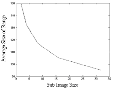
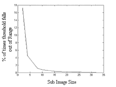
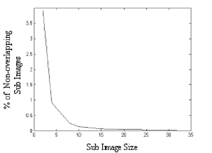
(a)                                       (b)                                       (c)

Figure 1: Plots showing dependence of three important characteristics on sub image size (averaged over 35 images)

We observed reduction in the average size of the range $R_{m,n}$ with increasing sub-image size. This can be seen from Fig. 1a. This reduction in size is because of the availability of elements nearer to $T_{m,n}$ in the bordering array $\it X$, when the sub-image size gets bigger. Since the algorithm starts from $S_{1,1}$ and propagates downwards, it is preferable to binarize $S_{1,1}$ with threshold obtained by applying threshold over the whole image.

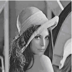
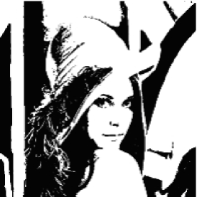
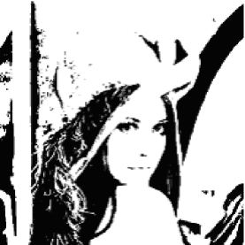
(a)                                     (b)                                     (c)

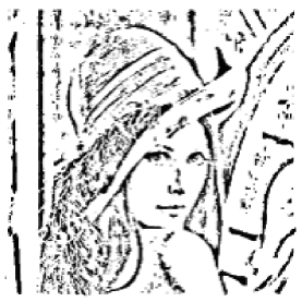
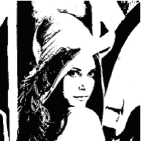
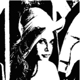
(d)                                     (e)                                     (f)

Figure 2: Comparison between the results of various methods, (a) Original image, (b) Thresholded using ADCDF, (c) Thresholded using Otsu, (d) Thresholded using Niblack, (e) Thresholded using ADCDF with LABT, (f) Thresholded using Otsu with LABT.

The second plot (Fig. 1b) shows the variation of the fraction of times threshold exceeds the range constraint; with sub-image size averaged over 35 images. The fraction of times $OT_{m,n}$ falling outside $R_{m,n}$ decreases with increase in sub-image size. This is due to stabilization of threshold across sub-images, when the sub-image size is increased. This is as expected, given the large-scale homogeneity present in numerous images.

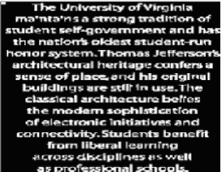
(a)                                                     (b)

Figure 3: (a) Original text image, (b) Thresholded using LABT.

We are presenting a few images for which the familiar method of thresholding, i.e., area division of cumulative distribution function (ADCDF), is used to binarize the sub-images. We have also used Otsu’s algorithm for the same purpose. Superior thresholding methods, when used in conjunction with this algorithm, will give far better results. For the purpose of illustrating the efficacy of our procedure and comparison, we have also presented the binarized images, using Otsu (global) and Niblack (local) thresholding methods in Fig. 2. One clearly sees that the present locally adaptive block thresholding method clearly does well in terms of extracting local features as well as retaining the visual image quality. We have checked this property of LABT in a variety of images.

Table 1
Quantitative comparision of various thresholding methods

(a)                                     (b)

(c)                                     (d)

Figure 4: (a) Original image, (b) Inverted threshold, (c) Thresholded image, and (d) Final image obtained after ORing.

For text images, thresholding followed by morphological operation like thinning gives good results (Fig. 3a & Fig 3b). It is advisable to choose the sub-image size to be more than the average object size in the image. This ensures the whole object, to be uniformly classified as background or foreground, and avoids classification of within-object variation.

The computational time and PSNR for different thresholding techniques, implemented with and without the locally adaptive block thresholding (LABT), has been shown in table 1. It is quite obvious from the results that the standard thresholding techniques fare better when applied in conjunction with our algorithm. The table also shows that the number of times threshold exceeds the range, and number of times the range dictated by upper and side sub-image does not overlap for three different thresholding algorithms are quite small. This justifies our assumption of exploiting the freedom of range for bringing out local details.

To avoid possible errors arising from the scanning of the image, row-wise from top to bottom, one can scan the image in different ways and perform an ORing operation of the different images, as specified below:

1) Image is thresholded in the usual way.

2) Invert the original image upside down and threshold the image. Then invert it back to the original state.

3) Invert the given image right side left and threshold the image. Then invert it back.

4) ORing operation is carried out on the above images to get the resulting image, which is equivalent to scanning the image in different ways and ORing them. Not just scanning row-wise from top to bottom.

The results of the ORing operation thus give superior results as shown in Fig. 4. One can see much clearer local details in the final image.

5 Conclusion and Discussion

In this paper, a new locally adaptive block thresholding method has been proposed, which acts as a hybrid between known local and global methods. It can also be used in conjunction with other methods of binarization to bring out details of an image. It should be emphasized that the same is accomplished without introducing too much of time complexity, an extremely desired attribute of any binarization scheme. The present algorithm has been designed to ensure that the transitions between sub-windows are maintained continuously. This maintains image continuity.

The efficacy of the method has been demonstrated in the context of a variety of images of different types. This procedure may also be useful when a variable window size is required. The portions of an image requiring detailed investigations may be divided into finer sub images, whereas other portions of the image can be divided into bigger box sizes. In this case, one needs to explore the problem of boundary mismatch and continuity more carefully. The boundary mismatch can be possibly taken care by pushing the boundary of the block that created the mismatch, till the selected threshold falls within the range. This problem is currently under investigation and will be reported elsewhere.

References

- [1] Abutaleb, A. S., 1989. Automatic Thresholding of Gray-level Pictures Using Two-Dimensional Entropy, Computer Vision Graphics and Image Processing, 47, 22-32.
- [2] Arora, S., Acharya, J., Verma, A., Panigrahi, P., 2005. Multilevel thresholding for image Segmantation through a Fast Statistical Recursive Algorithm. arXiv:cs.CV/0602044.
- [3] Chang, C. H., Tian, H., Srikanthan, T., Lim, C. S., 2002. Field programmable gate array based architecture for real time image segmentation by region growing algorithm, Journal of Electronic Imaging, 11 (4), 469-478.
- [4] Dawoud, A., Kamel, M., 2001. Binarization of document images using image dependent model. International Conference on Document Analysis and Recognition (ICDAR), Seattle, U.S.A , 49-53.
- [5] Gorman, L. O’, 1994. Binarization and Multi-thresholding of Document Images using Connectivity, Graphical Models and Image Processing, 56, 494-506.
- [6] Hertz, L., Schafer, R. W., 1998. Multilevel Thresholding Using Edge Matching, Computer Vision Graphics and Image Processing, 44, 279-295.
- [7] Huang, Q., Gai, W., Cai, W., 2005. Thresholding technique with adaptive window selection for uneven lighting image. Pattern Recognition Letters 26, 801-808.
- [8] Kapur, J. N., Sahoo, P. K., Wong, A. K. C., 1985. A New Method for Gray-level Picture Thresholding Using the Entropy of the histogram, Graphical Models and Image Processing, 29, 273-285.
- [9] Kittler, J., Illingworth, J., 1986. Minimum Error Thresholding, Pattern Recognition, 19, 41-47.
- [10] Leung, C. K. , Lam, F. K.,1996. Performance analysis of class of iterative image thresholding algorithms, Pattern Recognition, 29(9), 1523-1530.
- [11] Li, C. H., Lee, C. K., 1993. Minimum Cross-Entropy Thresholding, Pattern Recognition, 26, 617-625.
- [12] Li, C. H., Tam, P. K. S., 1998. An Iterative Algorithm for Minimum Cross -Entropy Thresholding, Pattern Recognition Letters, 19, 771-776.
- [13] Niblack, W., 1986. An Introduction to Image Processing, Prentice-Hall, 115-116.
- [14] Oh, W., Lindquist, B., 1999. Image thresholding by indicator kringing, IEEE Trans. Pattern Analysis and Machine Intelligence, PAMI, 21, 590-602.
- [15] Otsu, N., 1979. A threshold selection method from gray level histograms, IEEE Transactions on Systems, Man and Cybernetics, 9, 62-66.
- [16] Pal, N. R., Pal, S. K., 1989. Entropic Thresholding, Signal Processing, 16, 97-108.
- [17] Pun, T., 1980. A New Method for Gray -Level Picture Threshold Using the Entropy of the Histogram, Signal Processing, 2 (3), 223-237.
- [18] Ramesh, N., Yoo, J. H., Sethi, I. K., 1995. Thresholding Based on Histogram Approximation, IEE Proc.Vis.Image, Signal Proc., 142 (5), 271-279.
- [19] Ridler, T. W., Calvard, S., 1978. Picture thresholding using an iterative selection method, IEEE Trans. System, Man and Cybernetics, SMC-8, 630-632.
- [20] Rosenfeld, A., De La Torre, P., 1983. Histogram Concavity Analysis as an Aid in Threshold Selection, IEEE Trans System, Man and Cybernetics, SMC-13, 231-235.
- [21] Sahoo, P. K., Soltani, S., Wong, A. K. C., Chen, Y., 1998. A survey of Thresholding Techniques, Computer Graphics and Image Processing, 41, 233-260.
- [22] Sezan, M. I., 1985. A Peak Detection Algorithm and its Application to Histogram Based Image Data Reduction, Graphical Models and Image Processing, 29, 47-59.
- [23] Sezgin, M., Sankur, B., 2001. Comparison of Thresholding methods for non-destructive testing applications, International Conference on Image Processing IEEE ICIP’01, Thessaloniki, Greece.
- [24] Sezgin, M., Sankur., B, 2004. Survey over image thresholding techniques and quantative performance evaluation. Journal of Electronic Imaging, 13(1), 146-167.
- [25] Trier, O., Jain, A., 1995. Goal-directed evaluation of binarization methods, IEEE Tran. Pattern Analysis and Machine Intelligence, 7, 1191-1201.
- [26] Trier, O. D., Taxt, T., 1995. Evaluation of binarization methods for document images, IEEE Trans. Pattern Analysis and Machine Intelligence, PAMI, 312-315.
- [27] Tsai, W. H., 1985. Moment-preserving thresholding: A new approach, Graphical Models and Image Processing, 19, 377-393.
- [28] Wang, Q., Chi, Z., Zhao, R., 2002. Image thresholding by maximizing of non-fuzziness of the 2D grayscale histogram. Computer Image and Vision Understanding, 85, 100-116.
- [29] White, J. M., Rohrer, G. D., 1983. Image Thresholding for Optical Character Recognition and Other Application Requiring Character Image Extraction, IBM J Res. Develop, 27 (4), 400-411.