Quantization Bounds on Grassmann Manifolds and Applications to MIMO Communications${}^{{}^{*}}$

Abstract

This paper considers the quantization problem on the Grassmann manifold $\mathcal{G}_{n,p}$, the set of all $p$-dimensional planes (through the origin) in the $n$-dimensional Euclidean space. The chief result is a closed-form formula for the volume of a metric ball in the Grassmann manifold when the radius is sufficiently small. This volume formula holds for Grassmann manifolds with arbitrary dimension $n$ and $p$, while previous results pertained only to $p=1$, or a fixed $p$ with asymptotically large $n$. Based on this result, several quantization bounds are derived for sphere packing and rate distortion tradeoff. We establish asymptotically equivalent lower and upper bounds for the rate distortion tradeoff. Since the upper bound is derived by constructing random codes, this result implies that the random codes are asymptotically optimal. The above results are also extended to the more general case, in which $\mathcal{G}_{n,q}$ is quantized through a code in $\mathcal{G}_{n,p}$, where $p$ and $q$ are not necessarily the same. Finally, we discuss some applications of the derived results to multi-antenna communication systems.

I Introduction

The Grassmann manifold $\mathcal{G}_{n,p}\left(\mathbb{L}\right)$ is the set of all $p$-dimensional planes (through the origin) in the $n$-dimensional Euclidean space $\mathbb{L}^{n}$, where $\mathbb{L}$ is either $\mathbb{R}$ or $\mathbb{C}$. It forms a compact Riemann manifold of real dimension $\beta p\left(n-p\right)$, where $\beta=1$ when $\mathbb{L}=\mathbb{R}$ and $\beta=2$ when $\mathbb{L}=\mathbb{C}$. The Grassmann manifold provides a useful analysis tool for multi-antenna communications (also known as multiple-input multiple-output (MIMO) communication systems). For non-coherent MIMO systems, sphere packings of $\mathcal{G}_{n,p}\left(\mathbb{L}\right)$ can be viewed as a generalization of spherical codes [1, 2, 3]. For MIMO systems with partial channel state information at the transmitter (CSIT), which is obtained by finite-rate channel-state feedback, the quantization of beamforming matrices is related to the quantization on the Grassmann manifold [4, 5, 6].

The basic quantization problems addressed in this paper are the sphere packing bounds and rate distortion tradeoff. Roughly speaking, a quantization is a representation of a source in $\mathcal{G}_{n,p}\left(\mathbb{L}\right)$. In particular, it maps an element in $\mathcal{G}_{n,p}\left(\mathbb{L}\right)$ into a subset of $\mathcal{G}_{n,p}\left(\mathbb{L}\right)$, known as a code $\mathcal{C}$. Define the minimum distance of a code $\delta\triangleq\delta\left(\mathcal{C}\right)$ as the minimum distance between any two codewords in the code $\mathcal{C}$. A sphere packing bound relates the size of a code and a given minimum distance $\delta$. Rate distortion tradeoff is another important aspect of the quantization problem. A distortion metric is a mapping from the set of element pairs in $\mathcal{G}_{n,p}\left(\mathbb{L}\right)$ into the set of non-negative real numbers. Given a source distribution and a distortion metric, the rate distortion tradeoff is described by the minimum expected distortion achievable for a given code size, or equivalently the minimum code size required to achieve a particular expected distortion.

There are several papers addressing the quantization problem for Grassmann manifolds. In [7], an isometric embedding of $\mathcal{G}_{n,p}\left(\mathbb{R}\right)$ into a sphere in Euclidean space $\mathbb{R}^{\frac{1}{2}\left(m-1\right)\left(m+2\right)}$ is given. Then, using the Rankin bound in Euclidean space, the Rankin bound in $\mathcal{G}_{n,p}\left(\mathbb{R}\right)$ is obtained. Unfortunately, this bound is not tight when the code size is large. Instead of resorting to an isometric embedding, sphere packing bounds can also be derived from analysis in the Grassmann manifold directly. Let $B\left(\delta\right)$ denote a metric ball of radius $\delta$ in $\mathcal{G}_{n,p}\left(\mathbb{L}\right)$. The sphere packing bounds can be derived from the volume of $B\left(\delta\right)$ [3]. The exact volume formula for a $B\left(\delta\right)$ in $\mathcal{G}_{n,p}\left(\mathbb{L}\right)$ with $p=1$ and $\mathbb{L}=\mathbb{C}$ is derived in [4]. An asymptotic volume formula for a $B\left(\delta\right)$ in $\mathcal{G}_{n,p}\left(\mathbb{L}\right)$, where $p\geq 1$ is fixed and $n$ approaches infinity, is derived in [3]. Based on those volume formulas, the corresponding sphere packing bounds are developed in [5, 3]. Besides the sphere packing bounds, the rate distortion tradeoff is also treated in [8], where approximations to the distortion rate function are derived via the sphere packing bounds on the Grassmann manifold. However, the derived approximations are based on the volume formulas in [3, 4] which are only valid for some special choices of $n$ and $p$: either $p=1$ or fixed $p\geq 1$ with asymptotic large $n$.

The main contribution of this paper is to derive a closed-form formula for the volume of a small ball in the Grassmann manifold. Based on this formula, sphere packing bounds are derived and rate distortion tradeoff are accurately quantified. Specifically:

1. An explicit volume formula for a metric ball in $\mathcal{G}_{n,p}\left(\mathbb{L}\right)$ is derived when the radius $\delta$ is sufficiently small. It holds for Grassmann manifolds with arbitrary dimensions while previous results are only valid for either $p=1$ or a fixed $p$ with asymptotically large $n$. The main order term of the volume is $c_{n,p,p,\beta}\delta^{\beta p\left(n-p\right)}$ for a constant $c_{n,p,p,\beta}$ depending on $n$, $p$ and $\beta$. Lower and upper bounds on the volume formula are also derived.

2. Based on the volume formula, the Gilbert-Varshamov and Hamming bounds for sphere packings are obtained. For the distortion rate function, a lower bound is established via sphere packing argument and an upper bound is derived via random-code argument. The bounds are in fact asymptotically identical, and so precisely quantify the asymptotic rate distortion tradeoff. Since the upper bound is actually derived from the average distortion of random codes, it follows that random codes are asymptotically optimal.

3. The volume formula and the results on the rate distortion tradeoff are extended to a more general plane matching problem. In this plane matching problem, a plane from the code $\mathcal{C}\subset\mathcal{G}_{n,p}\left(\mathbb{L}\right)$ is chosen to match a random plane $Q\in\mathcal{G}_{n,q}\left(\mathbb{L}\right)$ to minimize the distortion, where $p$ and $q$ are not necessarily the same. For plane matching, a metric ball in $\mathcal{G}_{n,q}\left(\mathbb{L}\right)$ centered at a plane in $\mathcal{G}_{n,p}\left(\mathbb{L}\right)$ is studied. The volume formula is derived for such a ball with sufficiently small radius. The rate distortion tradeoff is also quantified by the same method as above.

4. As an application of the derived quantization bounds, the information rate of a MIMO system with finite-rate channel-state feedback and power on/off strategy is accurately quantified for the first time. Since the corresponding Grassmann manifold for most practical MIMO systems has $p>1$ and small $n$, the quantization bounds derived in this paper are necessary.

The paper is organized as follows. Section II provides some preliminaries on the Grassmann manifold. Section III derives the explicit volume formula for a metric ball in the Grassmann manifold. The corresponding sphere packing bounds are obtained and the rate distortion tradeoff is accurately quantified in Section IV. An application of the quantization bounds to MIMO systems with finite-rate channel-state feedback is detailed in Section V. Section VI contains the conclusions.

II Preliminaries

This section presents a brief introduction to the Grassmann manifold. A metric and a measure on the Grassmann manifold are defined, and the problems relevant to quantization on the Grassmann manifold are formulated. For completeness, we also extend the quantization problem to a more general plane matching problem.

II-A Metric and Measure on $\mathcal{G}_{n,p}\left(\mathbb{L}\right)$

For the sake of applications [4, 5, 6], the projection Frobenius metric (chordal distance) is employed throughout the paper although the corresponding analysis is also applicable to the geodesic metric [3]. For any two planes $P,Q\in\mathcal{G}_{n,p}\left(\mathbb{L}\right)$, we define the principle angles and the chordal distance between $P$ and $Q$ as follows. Let $\mathbf{u}_{1}\in P$ and $\mathbf{v}_{1}\in Q$ be the unit vectors such that $\left|\mathbf{u}_{1}^{\dagger}\mathbf{v}_{1}\right|$ is maximal. Inductively, let $\mathbf{u}_{i}\in P$ and $\mathbf{v}_{i}\in Q$ be the unit vectors such that $\mathbf{u}_{i}^{\dagger}\mathbf{u}_{j}=0$ and $\mathbf{v}_{i}^{\dagger}\mathbf{v}_{j}=0$ for all $1\leq j<i$ and $\left|\mathbf{u}_{i}^{\dagger}\mathbf{v}_{i}\right|$ is maximal. The principle angles are defined as $\theta_{i}=\arccos\left|\mathbf{u}_{i}^{\dagger}\mathbf{v}_{i}\right|$ for $i=1,\cdots,p$ [7, 9]. The chordal distance between $P$ and $Q$ is given by

$$d_{c}\left(P,Q\right)\triangleq\sqrt{\sum_{i=1}^{p}\sin^{2}\theta_{i}}.$$ (1)

The invariant measure $\mu$ on $\mathcal{G}_{n,p}\left(\mathbb{L}\right)$ is defined as follows. Let $O\left(n\right)$ and $U\left(n\right)$ be the groups of $n\times n$ orthogonal and unitary matrices respectively. Let $\mathbf{A},\mathbf{B}\in O\left(n\right)$ when $\mathbb{L}=\mathbb{R}$, or $\mathbf{A},\mathbf{B}\in U\left(n\right)$ when $\mathbb{L}=\mathbb{C}$. For any measurable set $\mathcal{M}\subset\mathcal{G}_{n,p}\left(\mathbb{L}\right)$ and arbitrary $\mathbf{A}$ and $\mathbf{B}$,

$$\mu\left(\mathbf{A}\mathcal{M}\right)=\mu\left(\mathcal{M}\right)=\mu\left(\mathcal{M}\mathbf{B}\right).$$

The invariant measure defines the uniform/isotropic distribution on $\mathcal{G}_{n,p}\left(\mathbb{L}\right)$ as well [9].

II-B Quantization on $\mathcal{G}_{n,p}\left(\mathbb{L}\right)$

Given both a metric and a measure on $\mathcal{G}_{n,p}\left(\mathbb{L}\right)$, a quantization on the Grassmann manifold can be well defined. Let $\mathcal{C}$ be a finite size discrete subset of $\mathcal{G}_{n,p}\left(\mathbb{L}\right)$. A quantization is a mapping from the $\mathcal{G}_{n,p}\left(\mathbb{L}\right)$ to the set $\mathcal{C}$ (also known as a code), i.e.,

$$\mathfrak{q}:\mathcal{G}_{n,p}\left(\mathbb{L}\right)\rightarrow\mathcal{C}.$$

An element in the code $\mathcal{C}$ is called a codeword. Thus, roughly speaking, a quantization is to use a subset of $\mathcal{G}_{n,p}\left(\mathbb{L}\right)$ to represent the whole space.

Sphere packing bounds relate the size of the code to the minimum distance among the codewords. Let $\delta$ be the minimum distance between any two codewords of a code $\mathcal{C}$ and $B\left(\delta\right)$ be a metric ball of radius $\delta$ in the $\mathcal{G}_{n,p}\left(\mathbb{L}\right)$. If $K$ is any positive integer such that $K\mu\left(B\left(\delta\right)\right)<1$, then there exists a code $\mathcal{C}$ of size $K+1$ with minimum distance $\delta$. This principle is called as the Gilbert-Varshamov lower bound,

$$\left|\mathcal{C}\right|>\frac{1}{\mu\left(B\left(\delta\right)\right)}.$$ (2)

On the other hand, $\left|\mathcal{C}\right|\mu\left(B\left(\delta/2\right)\right)\leq 1$ for any code $\mathcal{C}$. The Hamming upper bound captures this fact as

$$\left|\mathcal{C}\right|\leq\frac{1}{\mu\left(B\left(\delta/2\right)\right)}.$$ (3)

For more information about the sphere packing bounds, see [3].

Rate distortion tradeoff is another important aspect of the quantization problem. A distortion metric is a mapping,

$$\mathfrak{d}:\mathcal{G}_{n,p}\left(\mathbb{L}\right)\times\mathcal{C}\rightarrow\left[0,+\infty\right),$$

from the set of the element pairs in $\mathcal{G}_{n,p}\left(\mathbb{L}\right)$ and $\mathcal{C}$ into the set of non-negative real numbers. Throughout this paper, we define the distortion metric as the square of the chordal distance, $\mathfrak{d}\left(\cdot,\cdot\right)\triangleq d_{c}^{2}\left(\cdot,\cdot\right)$. Assume that a source $Q$ is randomly distributed in $\mathcal{G}_{n,p}\left(\mathbb{L}\right)$. The distortion associated with a quantization $\mathfrak{q}$ is defined as

$$D\triangleq\mathrm{E}\left[\mathfrak{d}\left(Q,\mathfrak{q}\left(Q\right)\right)\right]=\mathrm{E}\left[d_{c}^{2}\left(Q,\mathfrak{q}\left(Q\right)\right)\right].$$

The rate distortion tradeoff can be described by the infimum achievable distortion given a code size, which is called the distortion rate function, or equivalently the infimum code size required to achieve a particular distortion, which is called the rate distortion function. In this paper, the source $Q$ is assumed to be uniformly distributed in $\mathcal{G}_{n,p}\left(\mathbb{L}\right)$. For a given code $\mathcal{C}\subset\mathcal{G}_{n,p}\left(\mathbb{L}\right)$, the optimal quantization to minimize the distortion is given by

$$\mathfrak{q}\left(Q\right)=\arg\;\underset{P\in\mathcal{C}}{\min}\;d_{c}\left(P,Q\right).$$

The distortion associated with this quantization is

$$D\left(\mathcal{C}\right) = \mathrm{E}\left[\underset{P\in\mathcal{C}}{\min}\;d_{c}^{2}\left(P,Q\right)\right].$$

For a given code size $K$ where $K$ is a positive integer, the distortion rate function is then given by

$$D^{*}\left(K\right)=\underset{\mathcal{C}:\left|\mathcal{C}\right|=K}{\inf}\;D\left(\mathcal{C}\right).$$ (4)

The rate distortion function is given by

$$K^{*}\left(D\right)=\underset{D\left(\mathcal{C}\right)\leq D}{\inf}\;\left|\mathcal{C}\right|.$$ (5)

II-C An Extension: Plane Matching Problem

For the sake of completeness, we extend the quantization problem to a more general plane matching problem. The plane matching problem involves planes from different spaces $\mathcal{G}_{n,p}\left(\mathbb{L}\right)$ and $\mathcal{G}_{n,q}\left(\mathbb{L}\right)$ where $p$ and $q$ are not necessarily the same.

To formulate the plane matching problem, we need to define the chordal distance between $P\in\mathcal{G}_{n,p}\left(\mathbb{L}\right)$ and $Q\in\mathcal{G}_{n,q}\left(\mathbb{L}\right)$. Without loss of generality, we assume that $p\leq q$. Using the same procedure described in Section II-A, we are able to define the principle angles $0\leq\theta_{1}\leq\cdots\leq\theta_{p}\leq\frac{\pi}{2}$. Based on the principle angles, the chordal distance between $P\in\mathcal{G}_{n,p}\left(\mathbb{L}\right)$ and $Q\in\mathcal{G}_{n,q}\left(\mathbb{L}\right)$ are defined as $d_{c}\left(P,Q\right)\triangleq\sqrt{\sum_{i=1}^{p}\sin^{2}\theta_{i}}$. In this way, the definition of chordal distance in (1) is just a particular case of the general definition.

Now consider the plane matching problem. Intuitively, the plane matching problem is to choose a plane from the code $\mathcal{C}\subset\mathcal{G}_{n,p}\left(\mathbb{L}\right)$ to match a random plane $Q\in\mathcal{G}_{n,q}\left(\mathbb{L}\right)$ such that the average distortion is minimized, where $1\leq p\leq n$ and $1\leq q\leq n$ are not necessarily the same. Formally, a plane matching is a map from the whole space of Grassmann manifold, e.g., $\mathcal{G}_{n,q}\left(\mathbb{L}\right)$, to the code $\mathcal{C}\subset\mathcal{G}_{n,p}\left(\mathbb{L}\right)$,

$$\mathfrak{q}:\mathcal{G}_{n,q}\left(\mathbb{L}\right)\rightarrow\mathcal{C},$$

such that

$$D\left(\mathcal{C}\right)\triangleq\mathrm{E}_{Q}\left[\underset{P\in\mathcal{C}}{\min}\;d_{c}^{2}\left(P,Q\right)\right]$$

is minimized. According to the same principles in the quantization problem, the rate distortion tradeoff can be extended to the plane matching problem.

III Metric Balls in the Grassmann Manifold

In this section, an explicit volume formula for a metric ball $B\left(\delta\right)$ in the Grassmann manifold is derived. It is the essential tool to quantify the rate distortion tradeoff in Section IV.

The volume calculation depends on the relationship between the measure and the metric defined on the Grassmann manifold. This paper focuses on the invariant measure $\mu$, which corresponds to the uniform/isotropic distribution, and the chordal distance $d_{c}$. For any given $P\in\mathcal{G}_{n,p}\left(\mathbb{L}\right)$ and $Q\in\mathcal{G}_{n,q}\left(\mathbb{L}\right)$, define

$$B_{P}\left(\delta\right)=\left\{\hat{Q}\in\mathcal{G}_{n,q}\left(\mathbb{L}\right):\;d_{c}\left(P,\hat{Q}\right)\leq\delta\right\}$$

and

$$B_{Q}\left(\delta\right)=\left\{\hat{P}\in\mathcal{G}_{n,p}\left(\mathbb{L}\right):\;d_{c}\left(\hat{P},Q\right)\leq\delta\right\}.$$

For the invariant measure $\mu$, it has been shown that $\mu\left(B_{P}\left(\delta\right)\right)=\mu\left(B_{Q}\left(\delta\right)\right)$ and the value is independent of the choice of the center [9]. It is convenient to denote $B_{P}\left(\delta\right)$ and $B_{Q}\left(\delta\right)$ by $B\left(\delta\right)$ without distinguishing them. Then, the volume of a metric ball $B\left(\delta\right)$ is given by

$$\mu\left(B\left(\delta\right)\right)=\underset{\sum_{i=1}^{p}\sin^{2}\theta_{i}\leq\delta^{2}}{\int\cdots\int}\;d\mu_{\bm{\theta}},$$ (6)

where $1\leq\theta_{1}\leq\frac{\pi}{2},\cdots,1\leq\theta_{p}\leq\frac{\pi}{2}$ are the principle angles and the differential form $d\mu_{\bm{\theta}}$ is the joint density of the $\theta_{i}$’s, which is given in [9, 10, 11] and as well (20) in Appendix -A below.

The following theorem calculates the volume formula and expresses it as an exponentiation of the radius.

Theorem 1

When $\delta\leq 1$, the volume of a metric ball $B\left(\delta\right)$ is given by

$$\mu\left(B\left(\delta\right)\right)=c_{n,p,q,\beta}\delta^{\beta p\left(n-q\right)}\left(1+c_{n,p,q,\beta}^{\left(1\right)}\delta^{2}+o\left(\delta^{2}\right)\right),$$ (7)

where

$$\beta=\left\{\begin{array}[]{ll}1&\mathrm{if}\;\mathbb{L}=\mathbb{R}\\ 2&\mathrm{if}\;\mathbb{L}=\mathbb{C}\end{array}\right.,$$

$$c_{n,p,q,\beta}=\left\{\begin{array}[]{ll}\frac{1}{\Gamma\left(\frac{\beta}{2}p\left(n-q\right)+1\right)}\prod_{i=1}^{p}\frac{\Gamma\left(\frac{\beta}{2}\left(n-i+1\right)\right)}{\Gamma\left(\frac{\beta}{2}\left(q-i+1\right)\right)}&\mathrm{if}\;1\leq p\leq q\leq\frac{n}{2}\\ \frac{1}{\Gamma\left(\frac{\beta}{2}p\left(n-q\right)+1\right)}\prod_{i=1}^{p}\frac{\Gamma\left(\frac{\beta}{2}\left(n-i+1\right)\right)}{\Gamma\left(\frac{\beta}{2}\left(n-p-i+1\right)\right)}&\mathrm{if}\;1\leq p\leq\frac{n}{2}\leq q\leq n\;\mathrm{and}\;p+q\leq n\\ \frac{1}{\Gamma\left(\frac{\beta}{2}p\left(n-q\right)+1\right)}\prod_{i=1}^{n-q}\frac{\Gamma\left(\frac{\beta}{2}\left(n-i+1\right)\right)}{\Gamma\left(\frac{\beta}{2}\left(q-i+1\right)\right)}&\mathrm{if}\;1\leq p\leq\frac{n}{2}\leq q\leq n\;\mathrm{and}\;p+q\geq n\\ \frac{1}{\Gamma\left(\frac{\beta}{2}p\left(n-q\right)+1\right)}\prod_{i=1}^{n-q}\frac{\Gamma\left(\frac{\beta}{2}\left(n-i+1\right)\right)}{\Gamma\left(\frac{\beta}{2}\left(n-p-i+1\right)\right)}&\mathrm{if}\;\frac{n}{2}\leq p\leq q\leq n\end{array}\right.,$$ (8)

and

$$c_{n,p,q,\beta}^{\left(1\right)}=-\left(\frac{\beta}{2}\left(q-p+1\right)-1\right)\frac{\frac{\beta}{2}p\left(n-q\right)}{\frac{\beta}{2}p\left(n-q\right)+1}.$$ (9)

Proof:

See Appendix -A. ∎

The following corollary gives the two cases where the volume formula becomes exact.

Corollary 1

When $\delta\leq 1$, in either of the following two cases,

1. $\mathbb{L}=\mathbb{C}$ and $q=p$;

2. $\mathbb{L}=\mathbb{R}$ and $q=p+1$,

the volume of a metric ball $B\left(\delta\right)$ can be exactly calculated by

$$\mu\left(B\left(\delta\right)\right)=c_{n,p,q,\beta}\delta^{\beta p\left(n-q\right)},$$

where $c_{n,p,q,\beta}$ is defined in (8).

We also have the general bounds:

Corollary 2

Assume $\delta\leq 1$. If $\mathbb{L}=\mathbb{R}$ and $p=q$ , the volume of $B\left(\delta\right)$ is bounded by

$$c_{n,p,p,1}\delta^{p\left(n-p\right)}\leq\mu\left(B\left(\delta\right)\right)\leq c_{n,p,p,1}\delta^{p\left(n-p\right)}\left(1-\delta^{2}\right)^{-\frac{p}{2}}.$$

For all other cases,

$$\left(1-\delta^{2}\right)^{\frac{\beta}{2}p\left(q-p+1\right)-p}c_{n,p,q,\beta}\delta^{\beta p\left(n-q\right)}\leq\mu\left(B\left(\delta\right)\right)\leq c_{n,p,q,\beta}\delta^{\beta p\left(n-q\right)}.$$

Proof:

Corollary 1 and 2 follow the proof of Theorem 1 by tracking the higher order terms. ∎

Theorem 1 is of course consistent with the previous results in [4] and [3], which pertain to special choices of $n$ and $p$ and are stated below as examples.

Example 1

Consider the volume formula for a $B\left(\delta\right)$ where $p=q=1$. Without normalization, the total volume of $\mathcal{G}_{n,1}\left(\mathbb{C}\right)$ is $2\pi^{n}/\left(n-1\right)!$ and the volume of the $B\left(\delta\right)$ is $2\pi^{n}\delta^{2\left(n-1\right)}/\left(n-1\right)!$ [4]. Therefore,

$$\mu\left(B\left(\delta\right)\right)=\delta^{2\left(n-1\right)},$$

agreeing with Theorem 1 where $\beta=2$ and $c_{n,1,1,2}=1$.

Example 2

For the case that $p=q$ are fixed and $n\rightarrow+\infty$, an asymptotic volume formula for a $B\left(\delta\right)$ is derived by Barg [3], which reads

$$\mu\left(B\left(\delta\right)\right)=\left(\frac{\delta}{\sqrt{p}}\right)^{\beta np+o\left(n\right)}.$$ (10)

On the other hand, asymptotic analysis from Theorem 1 gives

$$\mu\left(B\left(\delta\right)\right)=\left(\frac{\delta}{\sqrt{p}}\right)^{\beta p\left(n-q\right)+O\left(\log n\right)}\left(1-\left(\frac{\beta}{2}\left(q-p+1\right)-1\right)\delta^{2}+o\left(\delta^{2}\right)\right)$$

for asymptotically large $n$ and any fixed $1\leq p\leq q$. The derivation follows the Stirling’s approximation applied to $-\frac{1}{\beta p\left(n-q\right)}\log\left(c_{n,p,q,\beta}\right)$. In this setting, Theorem 1 is consistent with (10) and provides refinement.

Importantly though, Theorem 1 is distinct from the above results in that it holds for arbitrary $p$, $q$ and $n$. For a metric ball with parameter $n$ not asymptotically large, i.e., $p$ and $q$ are comparable to $n$, it is not appropriate to use (10) to estimate the volume. A trivial example is that the $p=q=n$ case. If $p=q=n$, the exact volume of $B\left(\delta\right)$ for $\forall\delta>0$ is the constant $1$. The formula in Theorem 1 gives $c_{n,n,n,\beta}=1$ and $c_{n,n,n,\beta}\delta^{\beta p\left(n-q\right)}=1$. However, the approximation $\left(\delta/\sqrt{n}\right)^{\beta n^{2}}$ (formula (10)) will give a small number much less than $1$ when $\delta$ is small.

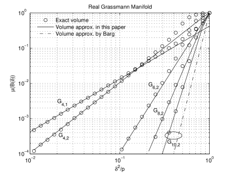
(a) Real Grassmann manifolds

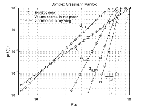
(b) Complex Grassmann manifolds

Figure 1: The volume of a metric ball in the Grassmann manifold

For engineering purposes, it may be satisfactory to approximate the volume of a metric ball $B\left(\delta\right)$ by $c_{n,p,q,\beta}\delta^{\beta p\left(n-q\right)}$ when the radius $\delta$ is relatively small. Fig. 1 compares the exact volume of a metric ball (6) and the volume approximation $c_{n,p,q,\beta}\delta^{\beta p\left(n-q\right)}$. In the simulations, we always assume $p=q$. The volume approximation becomes exact for the complex Grassmann manifold when $\delta\leq 1$. To calculate the exact volume without appealing to Theorem 1, Monte Carlo simulation is employed to evaluate the complicated integrals in (6). Since

$$\mu\left(B\left(\delta\right)\right)=\Pr\left\{Q:\;d_{c}\left(P,Q\right)\leq\delta\right\}$$

where $P\in\mathcal{G}_{n,p}\left(\mathbb{L}\right)$ is chosen arbitrarily and $Q$ is uniformly distributed in the $\mathcal{G}_{n,p}\left(\mathbb{L}\right)$, simulating the event $\left\{Q:\;d_{c}\left(P,Q\right)\leq\delta\right\}$ gives $\mu\left(B\left(\delta\right)\right)$. The simulation results for the real and complex Grassmann manifolds are presented in Fig. 1(a) and 1(b) respectively. Simulations show that the volume approximation (solid lines) is close to the exact volume (circles) when the radius of the metric ball is not large. We also compare our approximation with Barg’s approximation $\left(\delta/\sqrt{p}\right)^{\beta np}$ (from (10)) for the case $n=10$ and $p=2$. Simulations show that the exact volume and Barg’s approximation (dash-dot lines) may not be of the same order while the approximation in this paper is much more accurate.

IV Quantization Bounds

This section derives the sphere packing bounds and quantifies the rate distortion tradeoff for both quantization problem and plane matching problem. The results developed hold for Grassmann manifolds with arbitrary $n$, $p$ and $q$.

IV-A Sphere Packing Bounds

The Gilbert-Varshamov and Hamming bounds for $\mathcal{G}_{n,p}\left(\mathbb{L}\right)$ are given in the following corollary.

Corollary 3

When $\delta$ is sufficiently small ($\delta\leq 1$ necessarily), there exists a code $\mathcal{C}$ in the $\mathcal{G}_{n,p}\left(\mathbb{L}\right)$ with size $K$ and the minimum distance $\delta$ such that

$$c_{n,p,p,\beta}^{-1}\delta^{-\beta p\left(n-p\right)}\left(1+O\left(\delta^{2}\right)\right)\leq K.$$

For any code with the minimum distance $\delta$,

$$K\leq c_{n,p,p,\beta}^{-1}\left(\frac{\delta}{2}\right)^{-\beta p\left(n-p\right)}\left(1+O\left(\delta^{2}\right)\right).$$

Proof:

The corollary is proved by substituting the volume formula (7) into (2) and (3). ∎

Remark 1

Applying Corollary 2 would provide sharper information on the higher order term. But we omit this.

IV-B Quantization: the Rate Distortion Tradeoff

The rate distortion tradeoff for quantization is characterized in this subsection. Here, we assume that the quantization is on $\mathcal{G}_{n,p}\left(\mathbb{L}\right)$, the source is uniformly distributed in $\mathcal{G}_{n,p}\left(\mathbb{L}\right)$ and the distortion metric is defined as the square of the chordal distance. The derivation is based on the volume formula in (7). A lower bound and an upper bound on the distortion rate function are established. Denote the size of the code by $K$. Then the lower and upper bounds are asymptotically identical when $p$ is fixed, $n$ and the code rate $\log_{2}K$ approach to infinity with a fixed ratio. Therefore, these bounds precisely quantify the asymptotic rate distortion tradeoff. Note that the upper bound is the average distortion of random codes. Random codes are asymptotically optimal.

The following theorem gives a lower bound and an upper bound on the distortion rate function.

Theorem 2

When $K$ is sufficiently large ($\left(c_{n,p,p,\beta}K\right)^{-\frac{2}{\beta p\left(n-p\right)}}\leq 1$ necessarily), the distortion rate function is bounded as in

$$\frac{\beta p\left(n-p\right)}{\beta p\left(n-p\right)+2}\left(c_{n,p,p,\beta}K\right)^{-\frac{2}{\beta p\left(n-p\right)}}\left(1+o\left(1\right)\right)\leq D^{*}\left(K\right)$$

$$\quad\quad\quad\leq\frac{2\Gamma\left(\frac{2}{\beta p\left(n-p\right)}\right)}{\beta p\left(n-p\right)}\left(c_{n,p,p,\beta}K\right)^{-\frac{2}{\beta p\left(n-p\right)}}\left(1+o\left(1\right)\right)$$ (11)

Remark 2

For engineering purposes, the main order terms in (11) are usually accurate enough to characterize the distortion rate function. The details of the $\left(1+o\left(1\right)\right)$ correction are spelled out in Theorem 3 below, where a quantization is viewed as a specific case of plane matching.

The lower bound and the upper bound are proved in Appendix -B and -C respectively. We sketch the proof as follows.

The lower bound is proved by a sphere packing argument. The key is to construct an ideal quantizer, which may not exist, to minimize the distortion. Suppose that there exists $K$ metric balls of the same radius $\delta_{0}$ packing and covering the whole $\mathcal{G}_{n,p}\left(\mathbb{L}\right)$ at the same time. Then the quantizer which maps each of those balls into its center gives the minimum distortion among all quantizers. Of course such an ideal packing may not exist. It provides a lower bound on the distortion rate function.

The basic idea behind the upper bound is that the distortion of any particular code is an upper bound of the distortion rate function and so is the average distortion of an ensemble of codes. Toward the proof, the ensemble of random codes $\mathcal{C}_{\mathrm{rand}}=\left\{P_{1},\cdots,P_{K}\right\}$ are employed, where the codewords $P_{i}$’s are independently drawn from the uniform distribution on $\mathcal{G}_{n,p}\left(\mathbb{L}\right)$. For any given code $\mathcal{C}_{\mathrm{rand}}$, the corresponding distortion is given by

$$D\left(\mathcal{C}_{\mathrm{rand}}\right)=\mathrm{E}_{Q}\left[\underset{P_{i}\in\mathcal{C}_{\mathrm{rand}}}{\min}\;d_{c}^{2}\left(P_{i},Q\right)\right],$$

where $Q\in\mathcal{G}_{n,p}\left(\mathbb{L}\right)$ is a uniformly distributed plane. It is clear that $D^{*}\left(K\right)\leq\mathrm{E}_{\mathcal{C}_{\mathrm{rand}}}\left[D\left(\mathcal{C}_{\mathrm{rand}}\right)\right]$. We want to calculate $\mathrm{E}_{\mathcal{C}_{\mathrm{rand}}}\left[D\left(\mathcal{C}_{\mathrm{rand}}\right)\right]$. Note that

$$\mathrm{E}_{\mathcal{C}_{\mathrm{rand}}}\left[D\left(\mathcal{C}_{\mathrm{rand}}\right)\right] = \mathrm{E}_{\mathcal{C}_{\mathrm{rand}}}\left[\mathrm{E}_{Q}\left[\underset{P_{i}\in\mathcal{C}_{\mathrm{rand}}}{\min}\;d_{c}^{2}\left(P_{i},Q\right)\right]\right]$$

$$= \mathrm{E}_{Q}\left[\mathrm{E}_{\mathcal{C}_{\mathrm{rand}}}\left[\underset{P_{i}\in\mathcal{C}_{\mathrm{rand}}}{\min}\;d_{c}^{2}\left(P_{i},Q\right)\right]\right].$$

Since $\mathcal{C}_{\mathrm{rand}}$ is randomly generated from the uniform distribution, $\mathrm{E}_{\mathcal{C}_{\mathrm{rand}}}\left[\min\;d_{c}^{2}\left(P_{i},Q\right)\right]$ should be independent of the choice of $Q$. Therefore,

$$\mathrm{E}_{\mathcal{C}_{\mathrm{rand}}}\left[D\left(\mathcal{C}_{\mathrm{rand}}\right)\right]=\mathrm{E}_{\mathcal{C}_{\mathrm{rand}}}\left[\min\;d_{c}^{2}\left(P_{i},Q\right)\right]$$

for any fixed $Q$. By the volume formula and the extreme order statistics, we are able to calculate the distribution of $d_{c}^{2}\left(P_{i},Q\right)$ (for $\forall i$) and $\min\;d_{c}^{2}\left(P_{i},Q\right)$. In appendix -C, we prove that for any given $Q\in\mathcal{G}_{n,p}\left(\mathbb{L}\right)$, $K^{\frac{2}{t}}\cdot\mathrm{E}_{\mathcal{C}_{\mathrm{rand}}}\left[D\left(\mathcal{C}_{\mathrm{rand}}\right)\right]$ converges to a constant as $K$ approaches infinity. Therefore, an upper bound of the distortion rate function is obtained for asymptotically large $K$.

The rate distortion function is directly related to the distortion rate function. The following corollary quantifies the rate distortion function.

Corollary 4

When the required distortion $D$ is sufficiently small ($D\leq 1$ necessarily), the rate distortion function satisfies the following bounds,

$$\frac{1}{c_{n,p,p,\beta}}\left(\frac{\beta p\left(n-p\right)}{2\Gamma\left(\frac{2}{\beta p\left(n-p\right)}\right)}D\right)^{-\frac{\beta p\left(n-p\right)}{2}}\left(1+o\left(1\right)\right)\leq K^{*}\left(D\right)$$

$$\quad\quad\quad\leq\frac{1}{c_{n,p,p,\beta}}\left(\frac{\beta p\left(n-p\right)+2}{\beta p\left(n-p\right)}D\right)^{-\frac{\beta p\left(n-p\right)}{2}}\left(1+o\left(1\right)\right).$$ (12)

To investigate the difference between the lower and upper bounds in (11), proceed as follows. Since the exponential terms are the same in both bounds, focus on the coefficients. The difference between the two bounds depends on the number of real dimensions $\beta p\left(n-p\right)$ of the underlying Grassmann manifold. There are three cases to consider.

Case 1

$\beta p\left(n-p\right)=0$. This only occurs $n=p$. Then the whole $\mathcal{G}_{n,n}\left(\mathbb{L}\right)$ contains only one element and no quantization is needed essentially.

Case 2

$\beta p\left(n-p\right)=1$. This happens if and only if $\mathbb{L}=\mathbb{R}$, $n=2$ and $p=1$. In this case, it can be verified that the principle angle $\theta$ between a uniformly distributed $Q\in\mathcal{G}_{2,1}\left(\mathbb{R}\right)$ and any fixed $P\in\mathcal{G}_{2,1}\left(\mathbb{R}\right)$ is uniformly distributed in $\left[0,\frac{\pi}{2}\right]$. From here, the optimal quantization can be explicitly constructed. Since there exists $K$ metric balls with radius $\sin\frac{\pi}{4K}$ such that those balls not only pack but also cover the whole $\mathcal{G}_{2,1}\left(\mathbb{R}\right)$, the quantizer mapping those balls into its center is optimal. The distortion rate function can be explicitly calculated as

$$D^{*}\left(K\right)=\frac{1}{2K}-\frac{1}{\pi}\sin\frac{\pi}{2K}.$$

Case 3

$\beta p\left(n-p\right)\geq 2$. For this general case, an elementary calculation shows that

$$\frac{1}{2}\leq\frac{\beta p\left(n-p\right)}{\beta p\left(n-p\right)+2}\leq\frac{2}{\beta p\left(n-p\right)}\Gamma\left(\frac{2}{\beta p\left(n-p\right)}\right)\leq 1,$$

and we expect the difference between the two bounds to decrease as $n$ approaches infinity. Indeed, the following corollary shows that the lower and upper bounds are asymptotically the same.

Corollary 5

Suppose that $p$ is fixed, $n$ and the code rate $\log_{2}K$ approach to infinity simultaneously with $\bar{r}\triangleq\underset{\left(n,K\right)\rightarrow+\infty}{\lim}\frac{\log_{2}K}{n}$. If the normalized code rate $\bar{r}$ is sufficiently large ($p2^{-\frac{2}{\beta p}\bar{r}}\leq 1$ necessarily), then

$$\underset{\left(n,K\right)\rightarrow+\infty}{\lim}D^{*}\left(K\right)=p2^{-\frac{2}{\beta p}\bar{r}}.$$

On the other hand, if the required distortion $D$ is sufficiently small ($D\leq 1$ necessarily), then the minimum code size required to achieve that distortion satisfies

$$\underset{\left(n,K\right)\rightarrow+\infty}{\lim}\frac{\log_{2}K^{*}\left(D\right)}{n}=\frac{\beta p}{2}\log_{2}\left(\frac{p}{D}\right).$$

Proof:

The leading order is read off from

$$\underset{n\rightarrow+\infty}{\lim}\frac{\beta p\left(n-p\right)}{\beta p\left(n-p\right)+2}=1=\underset{n\rightarrow+\infty}{\lim}\frac{2}{\beta p\left(n-p\right)}\Gamma\left(\frac{2}{\beta p\left(n-p\right)}\right),$$

$$\underset{n\rightarrow+\infty}{\lim}\left(c_{n,p,p,\beta}\right)^{-\frac{2}{\beta p\left(n-p\right)}}=p,$$

$$\underset{\left(n,K\right)\rightarrow+\infty}{\lim}K^{-\frac{2}{p\left(n-p\right)}}=2^{-\frac{2}{\beta p}\bar{r}},$$

and

$$Kc_{n,p,p,\beta}\overset{\left(n,K\right)\rightarrow\infty}{\longrightarrow}\infty.$$

That the $\left(1+o\left(1\right)\right)$ multiplicative errors fall into place is the content of Theorem 3. ∎

The lower and upper bounds asymptotically agreeing accurately quantifies the distortion rate function. Since the upper bound is actually derived from the average distortion of random codes, this implies that random codes are asymptotically optimal.

As a comparison, we cite the distortion rate function approximation derived in [8]. For $\mathcal{G}_{n,p}\left(\mathbb{C}\right)$ with $p=1$, that paper offers the approximation

$$D^{*}\left(K\right)\approx\left(\frac{n-1}{n}\right)K^{-\frac{1}{n-1}}$$ (13)

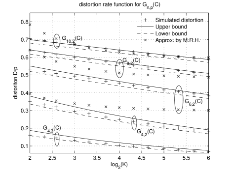
Figure 2: Bounds on the distortion rate function

by asymptotic arguments. According to our results in Theorem 2, the approximation (13) is indeed a lower bound for the distortion rate function and valid for all possible $n$’s. For $\mathcal{G}_{n,p}\left(\mathbb{C}\right)$ with $p$ fixed and $n\gg p$, a lower bound of an upper bound on the distortion rate function is given in [8] based on an estimation of the minimum distance of a code. It is less robust than the result in Theorem 2 in that it is neither a lower bound nor an upper bound, and it only holds for $n\gg p$ (see Fig. 2 for an empirical comparison).

Besides characterizing the rate distortion tradeoff, we are also interested in designing a code to minimize distortion for a given code size $K$. Generally speaking, it is computational complicated to design a code to minimize distortion directly. In [5] and [12], a suboptimal design criterion, i.e., maximization the minimum distance between codeword pairs, is proposed to reduce computational complexity. Refer this suboptimal criterion as max-min criterion. According to our volume formula (7), the same criterion can be verified. Let the minimum distance of a code $\mathcal{C}$ be $\delta$. Note that the metric balls of radius $\frac{\delta}{2}$ and centered at $P_{i}\in\mathcal{C}$ are disjoint. Then the corresponding distortion is upper bounded by

$$D\left(\mathcal{C}\right)\leq\frac{\delta^{2}}{4}K\mu\left(B\left(\delta/2\right)\right)+p\left(1-K\mu\left(B\left(\delta/2\right)\right)\right).$$ (14)

Apply the volume formula (7). An elementary calculation shows that the first derivative of the upper bound is negative when

$$\delta<\sqrt{\frac{4\beta p^{2}\left(n-p\right)}{2+\beta p\left(n-p\right)}}.$$

This property implies the upper bound (14) is a decreasing function of $\delta$ when $\delta$ is small enough. Thus, max-min criterion is an appropriate design criterion to obtain codes with small distortion. Since this criterion only requires to calculate the distance between codeword pairs, the computational complexity is less than that of designing a code to minimize the distortion directly.

Fig. 2 compares the simulated distortion rate function (the plus markers) with its lower bound (the dashed lines) and upper bound (the solid lines) in (11). To simulate the distortion rate function, we use the max-min criterion to design codes and use the minimum distortion of the designed codes as the distortion rate function. Simulation results show that the bounds in (11) hold for large $K$. When $K$ is relatively small, the formula (11) can serve as good approximations to the distortion rate function as well. Simulations also verify the previous discussion on the difference between the two bounds. The difference between the bounds is small and it becomes smaller as $n$ increases. In addition, we compare our bounds with the approximation (the “x” markers) derived in [8]. Simulations show that the approximation in [8] is neither an upper bound nor a lower bound. It works for the case that $n=10$ and $p=2$ but doesn’t work when $n\leq 8$ and $p=2$. As a comparison, the bounds (11) derived in this paper hold for arbitrary $n$ and $p$.

IV-C Plane Matching: the Rate Distortion Tradeoff

For completeness, this subsection summarizes the results about the rate distortion tradeoff for plane matching. The corresponding proofs follow those for the quantization problem.

Let a code $\mathcal{C}\in\mathcal{G}_{n,p}\left(\mathbb{L}\right)$. The plane matching problem is to choose a plane in $\mathcal{C}$ to match a random plane $Q\in\mathcal{G}_{n,q}\left(\mathbb{L}\right)$. Without loss of generality, we assume $1\leq p\leq q\leq n$. Denote the size of the code $\mathcal{C}$ by $K$. When $K$ is sufficient large, the distortion rate function is bounded by

$$\frac{\beta p\left(n-q\right)}{\beta p\left(n-q\right)+2}\left(c_{n,p,q,\beta}K\right)^{-\frac{2}{\beta p\left(n-q\right)}}\left(1+o\left(1\right)\right)\leq D^{*}\left(K\right)$$

$$\quad\quad\quad\leq\frac{2\Gamma\left(\frac{2}{\beta p\left(n-q\right)}\right)}{\beta p\left(n-q\right)}\left(c_{n,p,q,\beta}K\right)^{-\frac{2}{\beta p\left(n-q\right)}}\left(1+o\left(1\right)\right).$$

When the required distortion $D$ is sufficiently small, the rate distortion function is bounded by

$$\frac{1}{c_{n,p,q,\beta}}\left(\frac{\beta p\left(n-q\right)}{2\Gamma\left(\frac{2}{\beta p\left(n-q\right)}\right)}D\right)^{-\frac{\beta p\left(n-q\right)}{2}}\left(1+o\left(1\right)\right)\leq K^{*}\left(D\right)$$

$$\quad\quad\quad\leq\frac{1}{c_{n,p,q,\beta}}\left(\frac{\beta p\left(n-q\right)+2}{\beta p\left(n-q\right)}D\right)^{-\frac{\beta p\left(n-q\right)}{2}}\left(1+o\left(1\right)\right).$$

We finally detail the above $\left(1+o\left(1\right)\right)$ errors, and so those in (11) and (12) as well with the following theorem.

Theorem 3

Let $a$ be an arbitrary real number such that $0<a<1$ and $K$ be sufficiently large ($\left(c_{n,p,q,\beta}K\right)^{-\frac{2}{\beta p\left(n-q\right)}}\leq 1$ necessarily). If $\mathbb{L}=\mathbb{R}$ and $q=p$, then

$$\frac{p\left(n-p\right)}{p\left(n-p\right)+2}\left(c_{n,p,p,1}K\right)^{-\frac{2}{p\left(n-p\right)}}\left(1-\left(c_{n,p,p,1}K\right)^{-\frac{2}{p\left(n-p\right)}}\right)^{\frac{1}{n-p}}\leq D^{*}\left(K\right)$$

$$\quad\quad\leq\frac{2\Gamma\left(\frac{2}{p\left(n-p\right)}\right)}{p\left(n-p\right)}\left(Kc_{n,p,p,1}\right)^{-\frac{2}{p\left(n-p\right)}}+p\exp\left(-\left(Kc_{n,p,p,1}\right)^{1-a}\right).$$

If $\mathbb{L}=\mathbb{R}$ and $q=p+1$, or $\mathbb{L}=\mathbb{C}$ and $q=p$, then

$$\frac{\beta p\left(n-q\right)}{\beta p\left(n-q\right)+2}\left(c_{n,p,q,\beta}K\right)^{-\frac{2}{\beta p\left(n-q\right)}}\leq D^{*}\left(K\right)$$

$$\quad\quad\leq\frac{2\Gamma\left(\frac{2}{\beta p\left(n-q\right)}\right)}{\beta p\left(n-q\right)}\left(Kc_{n,p,q,\beta}\right)^{-\frac{2}{\beta p\left(n-q\right)}}+p\exp\left(-\left(Kc_{n,p,q,\beta}\right)^{1-a}\right).$$

If $\mathbb{L}=\mathbb{R}$ and $q>p+1$, or $\mathbb{L}=\mathbb{C}$ and $q>p$, then

$$\frac{\beta p\left(n-q\right)}{\beta p\left(n-q\right)+2}\left(c_{n,p,q,\beta}K\right)^{-\frac{2}{\beta p\left(n-q\right)}}\leq D^{*}\left(K\right)$$

$$\quad\quad\leq\frac{2\Gamma\left(\frac{2}{\beta p\left(n-q\right)}\right)}{\beta p\left(n-q\right)}\left(Kc_{n,p,q,\beta}\right)^{-\frac{2}{\beta p\left(n-q\right)}}\left(1-\left(Kc_{n,p,q,\beta}\right)^{-\frac{2a}{\beta p\left(n-q\right)}}\right)^{-\frac{\beta p\left(q-p+1\right)-2p}{\beta p\left(n-q\right)}}$$

$$\quad\quad\quad+p\exp\left(-\left(Kc_{n,p,q,\beta}\right)^{1-a}\left(1-\left(Kc_{n,p,q,\beta}\right)^{-\frac{2a}{\beta p\left(n-q\right)}}\right)^{\frac{\beta p\left(q-p+1\right)}{2}-p}\right).$$

Proof:

The proof is given in Appendix -B and -C. ∎

The lower and upper bounds are asymptotically identical. Let $p$ and $q$ be fixed. Let $n$ and the code rate $\log_{2}K$ approach to infinity simultaneously with $\bar{r}=\underset{\left(n,K\right)\rightarrow\infty}{\lim}\frac{\log_{2}K}{n}$. If the normalized code rate $\bar{r}$ is sufficiently large, then

$$\underset{\left(n,K\right)\rightarrow+\infty}{\lim}D^{*}\left(K\right)=p2^{-\frac{2}{\beta p}\bar{r}}.$$

On the other hand, if the required distortion $D$ is sufficiently small, then the minimum code size required to achieve that distortion satisfies

$$\underset{\left(n,K\right)\rightarrow+\infty}{\lim}\frac{\log_{2}K^{*}\left(D\right)}{n}=\frac{\beta p}{2}\log_{2}\left(\frac{p}{D}\right).$$

V An Application to MIMO Systems with Finite Rate Channel State Feedback

As an application of the derived quantization bounds on the Grassmann manifold, this section discusses the information theoretical benefit of finite-rate channel-state feedback for MIMO systems using power on/off strategy. In particular, we show that the benefit of the channel state feedback can be accurately characterized by the distortion of a quantization on the Grassmann manifold.

The effect of finite-rate feedback on MIMO systems using power on/off strategy has been widely studied. MIMO systems with only one on-beam are discussed in [4] and [5], where the beamforming codebook design criterion and performance analysis are derived by geometric arguments in the Grassmann manifold $\mathcal{G}_{n,1}\left(\mathbb{C}\right)$. MIMO systems with multiple on-beams are considered in [13, 14, 8, 15, 16]. Criteria to select the beamforming matrix are developed in [13] and [14]. The signal-to-noise ratio (SNR) loss due to quantized beamforming is discussed in [8]. The corresponding analysis is based on Barg’s formula (10) and only valid for MIMO systems with asymptotically large number of transmit antennas. The effect of beamforming quantization on information rate is investigated in [15] and [16]. The loss in information rate is quantified for high SNR region in [15]. That analysis is based on an approximation of the logdet function in the high SNR region and a metric on the Grassmann manifold other than the chordal distance. In [16], a formula to calculate the information rate for all SNR regimes is proposed by letting the numbers of transmit antennas, receive antennas and feedback rate approach infinity simultaneously. But this formula overestimates the performance in general.

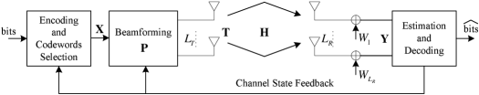
Figure 3: System model for a MIMO system

The basic model of a wireless communication system with $L_{T}$ transmit antennas, $L_{R}$ receive antennas and finite-rate channel state feedback is given in Fig. 3. The information bit stream is encoded into the Gaussian signal vector $\mathbf{X}\in\mathbb{C}^{s\times 1}$ and then multiplied by the beamforming matrix $\mathbf{P}\in\mathbb{C}^{L_{T}\times s}$ to generate the transmitted signal $\mathbf{T}=\mathbf{PX}$, where $s$ is the dimension of the signal $\mathbf{X}$ satisfying $1\leq s\leq L_{T}$ and the beamforming matrix $\mathbf{P}$ satisfies $\mathbf{P}^{\dagger}\mathbf{P}=\mathbf{I}_{s}$. In power on/off strategy, $\mathrm{E}\left[\mathbf{X}\mathbf{X}^{\dagger}\right]=P_{\mathrm{on}}\mathbf{I}_{s}$ where the $P_{\mathrm{on}}$ constant denotes the on-power. Assume that the channel $\mathbf{H}$ is Rayleigh flat fading, i.e., the entries of $\mathbf{H}$ are independent and identically distributed (i.i.d.) circularly symmetric complex Gaussian variables with zero mean and unit variance ($\mathcal{CN}\left(0,1\right)$) and $\mathbf{H}$ is i.i.d. for each channel use. Let $\mathbf{Y}\in\mathbb{C}^{L_{R}\times 1}$ be the received signal and $\mathbf{W}\in\mathbb{C}^{L_{R}\times 1}$ be the Gaussian noise, then

$$\mathbf{Y}=\mathbf{HPX}+\mathbf{W},$$

where $E\left[\mathbf{W}\mathbf{W}^{\dagger}\right]=\mathbf{I}_{L_{R}}$. We also assume that there is a beamforming codebook $\mathcal{B}=\left\{\mathbf{P}_{i}\in\mathbb{C}^{L_{T}\times s}:\right.$ $\left.\mathbf{P}_{i}^{\dagger}\mathbf{P}_{i}=\mathbf{I}_{s}\right\}$ declared to both the transmitter and the receiver before the transmission. At the beginning of each channel use, the channel state $\mathbf{H}$ is perfectly estimated at the receiver. A message, which is a function of the channel state, is sent back to the transmitter through a feedback channel. The feedback is error-free and rate limited. According to the channel state feedback, the transmitter chooses an appropriate beamforming matrix $\mathbf{P}_{i}\in\mathcal{B}$. Let the feedback rate be $R_{\mathrm{fb}}$bits/channel use. Then the size of the beamforming codebook $\left|\mathcal{B}\right|\leq 2^{R_{\mathrm{fb}}}$. The feedback function is a mapping from the set of channel state into the beamforming matrix index set, $\varphi:\;\left\{\mathbf{H}\right\}\rightarrow\left\{i:\;1\leq i\leq\left|\mathcal{B}\right|\right\}$. This section will quantify the corresponding information rate

$$\mathcal{I}=\underset{\mathcal{B}:\left|\mathcal{B}\right|\leq 2^{R_{\mathrm{fb}}}}{\max}\underset{\varphi}{\max}\;\mathrm{E}\left[\log\left|\mathbf{I}_{L_{R}}+P_{\mathrm{on}}\mathbf{H}\mathbf{P}_{\varphi\left(\mathbf{H}\right)}\mathbf{P}_{\varphi\left(\mathbf{H}\right)}^{\dagger}\mathbf{H}\right|\right],$$

where $P_{\mathrm{on}}=\rho/s$ and $\rho$ is the average received SNR.

Before discussing the finite-rate feedback case, we consider the case that the transmitter has full knowledge of the channel state $\mathbf{H}$. In this setting, the optimal beamforming matrix is given by $\mathbf{P}_{\mathrm{opt}}=\mathbf{V}_{s}$ where $\mathbf{V}_{s}\in\mathbb{C}^{L_{T}\times s}$ is the matrix composed by the right singular vectors of $\mathbf{H}$ corresponding to the largest $s$ singular values [6]. The corresponding information rate is

$$\mathcal{I}_{\mathrm{opt}}=\mathrm{E}_{\mathbf{H}}\left[\sum_{i=1}^{s}\mathrm{ln}\left(1+P_{\mathrm{on}}\lambda_{i}\right)\right],$$ (15)

where $\lambda_{i}$ is the $i^{\mathrm{th}}$ largest eigenvalue of $\mathbf{H}\mathbf{H}^{\dagger}$. In [6, Section III], we derive an asymptotic formula to approximate a quantity of the form $\mathrm{E}_{\mathbf{H}}\left[\sum_{i=1}^{s}\ln\left(1+c\lambda_{i}\right)\right]$ where $c>0$ is a constant. Apply the asymptotic formula in [6]. $\mathcal{I}_{\mathrm{opt}}$ can be well approximated.

The effect of finite-rate feedback can be characterized by the quantization bounds in the Grassmann manifold. For finite-rate feedback, we define a suboptimal feedback function

$$i=\varphi\left(\mathbf{H}\right)\triangleq\underset{1\leq i\leq\left|\mathcal{B}\right|}{\arg\ \min}\;d_{c}^{2}\left(\mathcal{P}\left(\mathbf{P}_{i}\right),\mathcal{P}\left(\mathbf{V}_{s}\right)\right),$$ (16)

where $\mathcal{P}\left(\mathbf{P}_{i}\right)$ and $\mathcal{P}\left(\mathbf{V}_{s}\right)$ are the planes in the $\mathcal{G}_{L_{T},s}\left(\mathbb{C}\right)$ generated by $\mathbf{P}_{i}$ and $\mathbf{V}_{s}$ respectively. In [6], we showed that this feedback function is asymptotically optimal as $R_{\mathrm{fb}}\rightarrow+\infty$ and near optimal when $R_{\mathrm{fb}}<+\infty$. With this feedback function and assuming that the feedback rate $R_{\mathrm{fb}}$ is large, it has also been shown in [6] that

$$\mathcal{I} \approx \mathrm{E}_{\mathbf{H}}\left[\sum_{i=1}^{s}\ln\left(1+\eta_{\sup}P_{\mathrm{on}}\lambda_{i}\right)\right],$$ (17)

where

$$\eta_{\sup} \triangleq 1-\frac{1}{s}\underset{\mathcal{B}:\left|\mathcal{B}\right|\leq 2^{R_{\mathrm{fb}}}}{\inf}\;\mathrm{E}_{\mathbf{V}_{s}}\left[\underset{1\leq i\leq\left|\mathcal{B}\right|}{\ \min}\;d_{c}^{2}\left(\mathcal{P}\left(\mathbf{P}_{i}\right),\mathcal{P}\left(\mathbf{V}_{s}\right)\right)\right]$$ (18)

$$= 1-\frac{1}{s}D^{*}\left(2^{R_{\mathrm{fb}}}\right).$$

Thus, the difference between perfect beamforming case (15) and finite-rate feedback case (17) is quantified by $\eta_{\sup}$, which depends on the distortion rate function on the $\mathcal{G}_{L_{T},s}\left(\mathbb{C}\right)$. Substituting quantization bounds (11) into (18) and applying the asymptotic formula in [6] for $\mathrm{E}_{\mathbf{H}}\left[\sum_{i=1}^{s}\ln\left(1+c\lambda_{i}\right)\right]$ produce approximations of the information rate $\mathcal{I}$ as a function of the feedback rate $R_{\mathrm{fb}}$.

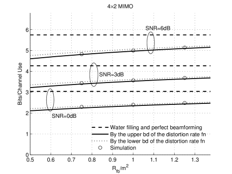
Figure 4: Performance of a constant number of on-beams v.s. feedback rate

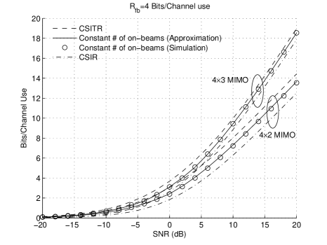
(a) Average mutual information

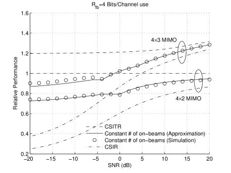
(b) Relative performance

Figure 5: Performance of a constant number of on-beams v.s. SNR

Simulations verify the above approximations. Let $m=\min\left(L_{T},L_{R}\right)$. Fig. 4 compares the simulated information rate (circles) and approximations as functions of $R_{\mathrm{fb}}/m^{2}$. The information rate approximated by the lower bound (solid lines) and the upper bound (dotted lines) in (11) are presented. The simulation results show that the performances approximated by the bounds (11) match the actual performance almost perfectly. As a comparison, the approximation proposed in [16, 17], which is based on asymptotic analysis and Gaussian approximation, overestimates the information rate. Furthermore, we compare the simulated information rate and the approximations for a large range of SNRs in Fig. 5. Without loss of generality, we only present the lower bound in (11) because it corresponds to the random codes and can be achieved by appropriate code design. Fig. 5(a) shows that the difference between the simulated and approximated information rate is almost unnoticeable. To make the performance difference clearer, Fig. 5(b) gives the relative performance as the ratio of the considered performance and the capacity of a $4\times 2$ MIMO achieved by water filling power control. The difference in relative performance is also small for all SNR regimes.

VI Conclusion

This paper considers the quantization problem on the Grassmann manifold. Based on an explicit volume formula for a metric ball in the $\mathcal{G}_{n,p}\left(\mathbb{L}\right)$, sphere packing bounds are obtained and the rate distortion tradeoff is accurately characterized by establishing bounds on the distortion function. Simulations verify the developed results. As an application of the derived quantization bounds, the information rate of a MIMO system with finite-rate channel-state feedback and power on/off strategy is accurately quantified for the first time.

-A Proof of Theorem 1

The proof is divided into three parts, in which we calculate the volume formula for the $1\leq p\leq q\leq\frac{n}{2}$, $\frac{n}{2}\leq p\leq q\leq n$ and $1\leq p\leq\frac{n}{2}\leq q\leq n$ cases respectively.

-A1 $1\leq p\leq q\leq\frac{n}{2}$ case

First we prove the basic form

$$\mu\left(B\left(\delta\right)\right)=c_{n,p,q,\beta}\delta^{\beta p\left(n-q\right)}\left(1+c_{n,p,q,\beta}^{\left(1\right)}\delta^{2}+o\left(\delta^{2}\right)\right)$$

for $\delta\leq 1$. Afterward, we calculate the constants $c_{n,p,q,\beta}$ and $c_{n,p,q,\beta}^{\left(1\right)}$.

The volume of a metric ball $\mu\left(B\left(\delta\right)\right)$ is given by

$$\mu\left(B\left(\delta\right)\right)=\underset{\sqrt{\sum_{i=1}^{p}\sin^{2}\theta_{i}}\leq\delta}{\int\cdots\int}\;d\mu_{\bm{\theta}},$$ (19)

where the differential form $d\mu_{\bm{\theta}}$ is the joint density of $\theta_{i}$’s. For convenience, we introduce the following notations. Define $r_{i}\triangleq\cos\theta_{i}$ and order $r_{i}$’s such that $r_{i}\leq r_{j}$ ($\theta_{i}\geq\theta_{j}$) if $i<j$. Define $\mathbf{r}=\left[r_{1},\cdots,r_{p}\right]$ and also

$$\left|\Delta_{p}\left(\mathbf{r}^{2}\right)\right|=\prod_{i<j}^{p}\left|r_{j}^{2}-r_{i}^{2}\right|.$$

Recall that $\beta=1$ for $\mathbb{L}=\mathbb{R}$ and $\beta=2$ for $\mathbb{L}=\mathbb{C}$. With these notations, the invariant measure $d\mu_{\bm{\theta}}$ can be written as follows [11].

$$d\mu_{\bm{\theta}}=v_{n,p,q,\beta}\left|\Delta_{p}\left(\mathbf{r}^{2}\right)\right|^{\beta}\prod_{i=1}^{p}\left(\left(r_{i}^{2}\right)^{\frac{\beta}{2}\left(q-p+1\right)-1}\left(1-r_{i}^{2}\right)^{\frac{\beta}{2}\left(n-p-q+1\right)-1}dr_{i}^{2}\right),$$ (20)

where the constant $v_{n,p,q,\beta}$ is given by

$$v_{n,p,q,\beta}=\prod_{i=1}^{p}\frac{\Gamma\left(1+\frac{\beta}{2}\right)\Gamma\left(\frac{\beta}{2}\left(n-i+1\right)\right)}{\Gamma\left(\frac{\beta}{2}i+1\right)\Gamma\left(\frac{\beta}{2}\left(n-p-i+1\right)\right)\Gamma\left(\frac{\beta}{2}\left(q-i+1\right)\right)}.$$ (21)

To get the form (7), we perform the variable change $\delta^{2}x_{i}=1-r_{i}^{2}$ for $1\leq i\leq p$. Under this transformation, the integral domain

$$D_{\delta}\triangleq\left\{\mathbf{r}:\;\sum\left(1-r_{i}^{2}\right)\leq\delta^{2},\;0\leq r_{i}^{2}\leq 1\;\mathrm{for}\;i=1,\cdots,p\right\}$$

is changed to

$$D_{1} \triangleq \left\{\mathbf{x}:\;\sum x_{i}\leq 1,\;0\leq x_{i}\leq\frac{1}{\delta^{2}}\;\mathrm{for}\;i=1,\cdots,p\right\}$$

$$= \left\{\mathbf{x}:\;\sum x_{i}\leq 1,\;0\leq x_{i}\;\mathrm{for}\;i=1,\cdots,p\right\},$$

where the last equation holds since $\delta\leq 1$. Thus

$$\mu\left(B\left(\delta\right)\right)=v_{n,p,q,\beta}\delta^{\beta p\left(n-q\right)}\underset{D_{1}}{\int\cdots\int}\left|\Delta\left(\mathbf{x}\right)\right|^{\beta}\prod_{i=1}^{p}\left(\left(1-\delta^{2}x_{i}\right)^{\frac{\beta}{2}\left(q-p+1\right)-1}\left(x_{i}\right)^{\frac{\beta}{2}\left(n-p-q+1\right)-1}dx_{i}\right).$$

Next note that

$$\left(1-\delta^{2}x_{i}\right)^{\frac{\beta}{2}\left(q-p+1\right)-1}=1-\left(\frac{\beta}{2}\left(q-p+1\right)-1\right)x_{i}\delta^{2}+o\left(\delta^{2}\right),$$

and so we are able to express the volume of $B\left(\delta\right)$ in the desired form with

$$c_{n,p,q,\beta}\triangleq v_{n,p,q,\beta}\underset{D_{1}}{\int\cdots\int}\left|\Delta\left(\mathbf{x}\right)\right|^{\beta}\prod_{i=1}^{p}\left(\left(x_{i}\right)^{\frac{\beta}{2}\left(n-p-q+1\right)-1}dx_{i}\right),$$

and

$$c_{n,p,q,\beta}^{\left(1\right)}\triangleq-p\cdot\left(\frac{\beta}{2}\left(q-p+1\right)-1\right)\frac{\underset{D_{1}}{\int\cdots\int}x_{1}\left|\Delta\left(\mathbf{x}\right)\right|^{\beta}\prod_{i=1}^{p}\left(\left(x_{i}\right)^{\frac{\beta}{2}\left(n-p-q+1\right)-1}dx_{i}\right)}{\underset{D_{1}}{\int\cdots\int}\left|\Delta\left(\mathbf{x}\right)\right|^{\beta}\prod_{i=1}^{p}\left(\left(x_{i}\right)^{\frac{\beta}{2}\left(n-p-q+1\right)-1}dx_{i}\right)}.$$

In order to calculate the constants $c_{n,p,q,\beta}$ and $c_{n,p,q,\beta}^{\left(1\right)}$, we need the following lemma [18].

Lemma 1

It holds that

$$\int\cdots\int x_{1}\cdots x_{m}\left|\Delta\left(\mathbf{x}\right)\right|^{\beta}\left(1-\sum_{i=1}^{p}x_{i}\right)^{\gamma-1}\prod_{i=1}^{p}x_{i}^{\alpha-1}dx_{i}$$

$$=\frac{\Gamma\left(\gamma\right)}{\Gamma\left(\gamma+m+\alpha p+\frac{\beta}{2}p\left(p-1\right)\right)}\prod_{i=1}^{m}\left(\alpha+\frac{\beta}{2}\left(p-i\right)\right)$$

$$\quad\times\prod_{i=1}^{p}\frac{\Gamma\left(\alpha+\frac{\beta}{2}\left(p-i\right)\right)\Gamma\left(1+\frac{\beta}{2}i\right)}{\Gamma\left(1+\frac{\beta}{2}\right)}.$$

where $0\leq m\leq p$, $\Re\left(\alpha\right)>0$, $\Re\left(\gamma\right)>0$, $\Re\left(\frac{\beta}{2}\right)>-\min\left(\frac{1}{p},\frac{\Re\left(\alpha\right)}{p-1},\frac{\Re\left(\gamma\right)}{p-1}\right)$ and the integral is taken over $0\leq x_{i},\;\sum_{i=1}^{p}x_{i}\leq 1$.

Proof:

This is Selberg’s second generalization of the beta integral. See [18, Section 17.10] for a detailed proof. ∎

According to Lemma 1, we have that

$$\underset{D_{1}}{\int\cdots\int}\left|\Delta\left(\mathbf{x}\right)\right|^{\beta}\prod_{i=1}^{p}\left(\left(x_{i}\right)^{\frac{\beta}{2}\left(n-p-q+1\right)-1}dx_{i}\right)$$

$$=\frac{1}{\Gamma\left(p\frac{\beta}{2}\left(n-p-q+1\right)+\frac{\beta}{2}p\left(p-1\right)+1\right)}$$

$$\quad\times\prod_{i=1}^{p}\frac{\Gamma\left(1+\frac{\beta}{2}i\right)\Gamma\left(\frac{\beta}{2}\left(n-p-q+1\right)+\frac{\beta}{2}\left(p-i\right)\right)}{\Gamma\left(1+\frac{\beta}{2}\right)}$$

$$=\frac{1}{\Gamma\left(\frac{\beta}{2}p\left(n-q\right)+1\right)}\prod_{i=1}^{p}\frac{\Gamma\left(1+\frac{\beta}{2}i\right)\Gamma\left(\frac{\beta}{2}\left(n-q-i+1\right)\right)}{\Gamma\left(1+\frac{\beta}{2}\right)}.$$

Substituting the formula (21) for $v_{n,p,q,\beta}$ into the integral expansion of $c_{n,p,q,\beta}$ yields

$$c_{n,p,q,\beta}=\frac{1}{\Gamma\left(\frac{\beta}{2}p\left(n-q\right)+1\right)}\prod_{i=1}^{p}\frac{\Gamma\left(\frac{\beta}{2}\left(n-i+1\right)\right)}{\Gamma\left(\frac{\beta}{2}\left(q-i+1\right)\right)}$$

after some simplifications.

The constant $c_{n,p,q,\beta}^{\left(1\right)}$ can be calculated in a similar way. Lemma 1 implies that

$$\underset{D_{1}}{\int\cdots\int}x_{1}\left|\Delta\left(\mathbf{x}\right)\right|^{\beta}\prod_{i=1}^{p}\left(\left(x_{i}\right)^{\frac{\beta}{2}\left(n-p-q+1\right)-1}dx_{i}\right)$$

$$=\frac{\frac{\beta}{2}\left(n-p-q+1\right)+\frac{\beta}{2}\left(p-1\right)}{\Gamma\left(\frac{\beta}{2}p\left(n-q\right)+2\right)}\prod_{i=1}^{p}\frac{\Gamma\left(1+\frac{\beta}{2}i\right)\Gamma\left(\frac{\beta}{2}\left(n-q-i+1\right)\right)}{\Gamma\left(1+\frac{\beta}{2}\right)}$$

$$=\frac{\frac{\beta}{2}\left(n-q\right)}{\frac{\beta}{2}p\left(n-q\right)+1}\left(\frac{1}{\Gamma\left(\frac{\beta}{2}p\left(n-q\right)+1\right)}\prod_{i=1}^{p}\frac{\Gamma\left(1+\frac{\beta}{2}i\right)\Gamma\left(\frac{\beta}{2}\left(n-q-i+1\right)\right)}{\Gamma\left(1+\frac{\beta}{2}\right)}\right).$$

Therefore,

$$c_{n,p,q,\beta}^{\left(1\right)}=-\left(\frac{\beta}{2}\left(q-p+1\right)-1\right)\frac{\frac{\beta}{2}p\left(n-q\right)}{\frac{\beta}{2}p\left(n-q\right)+1},$$

which completes the proof of the $1\leq p\leq q\leq\frac{n}{2}$ case.

-A2 $\frac{n}{2}\leq p\leq q\leq n$ case

This computation is closely related to that for the $1\leq p\leq q\leq\frac{n}{2}$ case.

To see the connection between the $\frac{n}{2}\leq p\leq q\leq n$ and $1\leq p\leq q\leq\frac{n}{2}$ cases, we define the generator matrix and the orthogonal complement plane. For any given plane $P\in\mathcal{G}_{n,p}\left(\mathbb{L}\right)$, the generator matrix $\mathbf{P}\in\mathbb{L}^{n\times p}$ is the matrix whose $p$ columns are orthonormal and expand the plane $P$. The generator matrix is not uniquely defined. However, the chordal distance between $P\in\mathcal{G}_{n,p}\left(\mathbb{L}\right)$ and $Q\in\mathcal{G}_{n,q}\left(\mathbb{L}\right)$ can be uniquely defined by their generator matrices. Indeed,

$$d_{c}^{2}\left(P,Q\right)=\min\left(p,q\right)-\mathrm{tr}\left(\mathbf{P}^{\dagger}\mathbf{Q}\mathbf{Q}^{\dagger}\mathbf{P}\right),$$

where $\mathbf{P}$ and $\mathbf{Q}$ are generator matrices for the plane $P$ and $Q$ respectively. It can be shown that the chordal distance is independent of the choice of the generator matrices. The orthogonal complement plane is defined as follows. For any given plane $P\in\mathcal{G}_{n,p}\left(\mathbb{L}\right)$, its orthogonal complement plane $P^{\perp}$ is the plane in $\mathcal{G}_{n,n-p}\left(\mathbb{L}\right)$ such that the minimum principle angle between $P$ and $P^{\perp}$ is $\frac{\pi}{2}$. It is straightforward that $\mathbf{P}^{\dagger}\mathbf{P}^{\perp}=\mathbf{0}$ where $\mathbf{P}$ and $\mathbf{P}^{\perp}$ are the generator matrices for $P$ and $P^{\perp}$ respectively, and the matrix $\mathbf{0}$ is the $p\times\left(n-p\right)$ matrix with all elements $0$.

With the definition of the orthogonal complement plane, the chordal distance between $P$ and $Q$ can be related to that between $P^{\perp}$ and $Q^{\perp}$. The relationship is given in the following lemma.

Lemma 2

For any given planes $P\in\mathcal{G}_{n,p}\left(\mathbb{L}\right)$ and $Q\in\mathcal{G}_{n,q}\left(\mathbb{L}\right)$, let $P^{\perp}\in\mathcal{G}_{n,n-p}\left(\mathbb{L}\right)$ and $Q^{\perp}\in\mathcal{G}_{n,n-q}\left(\mathbb{L}\right)$ be their orthogonal complement planes respectively. Then

$$d_{c}^{2}\left(P,Q\right)=d_{c}^{2}\left(P^{\perp},Q^{\perp}\right).$$

Proof:

This lemma can be proved by the generator matrices. Let $\mathbf{P}$, $\mathbf{Q}$, $\mathbf{P}^{\perp}$ and $\mathbf{Q}^{\perp}$ be the generator matrices for $P$, $Q$, $P^{\perp}$ and $Q^{\perp}$ respectively. Without loss of generality, we also assume that $1\leq p\leq q\leq n$. Then

$$p = \mathrm{tr}\left(\mathbf{P}^{\dagger}\left[\mathbf{Q}\mid\mathbf{Q}^{\perp}\right]\left[\mathbf{Q}\mid\mathbf{Q}^{\perp}\right]^{\dagger}\mathbf{P}\right)$$

$$= \mathrm{tr}\left(\mathbf{P}^{\dagger}\mathbf{Q}\mathbf{Q}^{\dagger}\mathbf{P}\right)+\mathrm{tr}\left(\mathbf{P}^{\dagger}\mathbf{Q}^{\perp}\left(\mathbf{Q}^{\perp}\right)^{\dagger}\mathbf{P}\right),$$

where the matrix $\left[\mathbf{Q}\mid\mathbf{Q}^{\perp}\right]$ is the one composed of $\mathbf{Q}$ and $\mathbf{Q}^{\perp}$. Similarly,

$$n-q = \mathrm{tr}\left(\left(\mathbf{Q}^{\perp}\right)^{\dagger}\left[\mathbf{P}\mid\mathbf{P}^{\perp}\right]\left[\mathbf{P}\mid\mathbf{P}^{\perp}\right]^{\dagger}\mathbf{Q}^{\perp}\right)$$

$$= \mathrm{tr}\left(\left(\mathbf{Q}^{\perp}\right)^{\dagger}\mathbf{P}\mathbf{P}^{\dagger}\mathbf{Q}^{\perp}\right)+\mathrm{tr}\left(\left(\mathbf{Q}^{\perp}\right)^{\dagger}\mathbf{P}^{\perp}\left(\mathbf{P}^{\perp}\right)^{\dagger}\mathbf{Q}^{\perp}\right).$$

Then

$$d_{c}^{2}\left(P,Q\right) \overset{\left(a\right)}{=} p-\mathrm{tr}\left(\mathbf{P}^{\dagger}\mathbf{Q}\mathbf{Q}^{\dagger}\mathbf{P}\right)$$

$$= \mathrm{tr}\left(\mathbf{P}^{\dagger}\mathbf{Q}^{\perp}\left(\mathbf{Q}^{\perp}\right)^{\dagger}\mathbf{P}\right)$$

$$= n-q-\mathrm{tr}\left(\left(\mathbf{Q}^{\perp}\right)^{\dagger}\mathbf{P}^{\perp}\left(\mathbf{P}^{\perp}\right)^{\dagger}\mathbf{Q}^{\perp}\right)$$

$$\overset{\left(b\right)}{=} d_{c}^{2}\left(P^{\perp},Q^{\perp}\right),$$

where (a) and (b) are from the definition of the chordal distance and the facts that $\min\left(p,q\right)=p$ and $\min\left(n-p,n-q\right)=n-q$. ∎

By this lemma, the connection between the $\frac{n}{2}\leq p\leq q\leq n$ case and $1\leq p\leq q\leq\frac{n}{2}$ case is clear. The volume formula for the $\frac{n}{2}\leq p\leq q\leq n$ case can be calculated as follows.

$$\mu\left(B_{P}\left(\delta\right)\right) = \Pr\left(Q\in\mathcal{G}_{n,q}\left(\mathbb{L}\right):\;d_{c}^{2}\left(P,Q\right)\leq\delta^{2}\right)$$

$$= \Pr\left(Q^{\perp}\in\mathcal{G}_{n,n-q}\left(\mathbb{L}\right):\;d_{c}^{2}\left(P^{\perp},Q^{\perp}\right)\leq\delta^{2}\right)$$

$$= \mu\left(B_{P^{\perp}}\left(\delta\right)\right)$$

where $B_{P}\left(\delta\right)$ and $B_{P^{\perp}}\left(\delta\right)$ are the metric balls in $\mathcal{G}_{n,q}\left(\mathbb{L}\right)$ and $\mathcal{G}_{n,n-q}\left(\mathbb{L}\right)$ respectively. Therefore, the results for the $1\leq p\leq q\leq\frac{n}{2}$ case can be directly applied by letting $p^{\prime}=n-q$ and $q^{\prime}=n-p$. Finally after some simplification, we have

$$\mu\left(B_{P}\left(\delta\right)\right) = c_{n,p,q,\beta}\delta^{\beta p\left(n-q\right)}\left(1+c_{n,p,q,\beta}^{\left(1\right)}\delta^{2}+o\left(\delta^{2}\right)\right),$$

where

$$c_{n,p,q,\beta}=\frac{1}{\Gamma\left(\frac{\beta}{2}p\left(n-q\right)+1\right)}\prod_{i=1}^{n-q}\frac{\Gamma\left(\frac{\beta}{2}\left(n-i+1\right)\right)}{\Gamma\left(\frac{\beta}{2}\left(n-p-i+1\right)\right)},$$

and

$$c_{n,p,q,\beta}^{\left(1\right)}=-\left(\frac{\beta}{2}\left(q-p+1\right)-1\right)\frac{\frac{\beta}{2}p\left(n-q\right)}{\frac{\beta}{2}p\left(n-q\right)+1}.$$

-A3 $1\leq p\leq\frac{n}{2}\leq q\leq n$ case

This computation is again related to that for the $1\leq p\leq q\leq\frac{n}{2}$ case.

Similar to the $\frac{n}{2}\leq p\leq q\leq n$ case, the connection between the $\frac{n}{2}\leq p\leq q\leq n$ case and $1\leq p\leq q\leq\frac{n}{2}$ case can be revealed by the generator matrix and the orthogonal complement plane. Let $p^{\prime}=\min\left(p,n-q\right)$ and $q^{\prime}=\max\left(p,n-q\right)$. Then $1\leq p^{\prime}\leq q^{\prime}\leq\frac{n}{2}$. For any given planes $P\in\mathcal{G}_{n,p}\left(\mathbb{L}\right)$ and $Q\in\mathcal{G}_{n,q}\left(\mathbb{L}\right)$, let $Q^{\perp}\in\mathcal{G}_{n,n-q}\left(\mathbb{L}\right)$ be the orthogonal complement plane of $Q$. Let $\mathbf{P}$, $\mathbf{Q}$ and $\mathbf{Q}^{\perp}$ be the generator matrices for $P$, $Q$ and $Q^{\perp}$. Then

$$d_{c}^{2}\left(P,Q\right) = p-\mathrm{tr}\left(\mathbf{P}^{\dagger}\mathbf{Q}\mathbf{Q}^{\dagger}\mathbf{P}\right)$$

$$= \mathrm{tr}\left(\mathbf{P}^{\dagger}\mathbf{Q}^{\perp}\left(\mathbf{Q}^{\perp}\right)^{\dagger}\mathbf{P}\right)$$

$$= p^{\prime}-d_{c}^{2}\left(P,Q^{\perp}\right).$$

Therefore,

$$\mu\left(B_{P}\left(\delta\right)\right) = \Pr\left(Q\in\mathcal{G}_{n,q}\left(\mathbb{L}\right):\;d_{c}^{2}\left(P,Q\right)\leq\delta^{2}\right)$$

$$= \Pr\left(Q^{\perp}\in\mathcal{G}_{n,n-q}\left(\mathbb{L}\right):\;d_{c}^{2}\left(P,Q^{\perp}\right)\geq p-\delta^{2}\right).$$

Now calculate the volume formula. Note that

$$\mu\left(B_{P}\left(\delta\right)\right)=\Pr\left(Q^{\perp}\in\mathcal{G}_{n,n-q}\left(\mathbb{L}\right):\;d_{c}^{2}\left(P,Q^{\perp}\right)\geq p^{\prime}-\delta^{2}\right).$$

Then

$$\mu\left(B_{P}\left(\delta\right)\right) = \underset{0\leq r_{i}^{2}\leq 1,\;\sum_{i=1}^{p^{\prime}}\left(1-r_{i}^{2}\right)\geq p^{\prime}-\delta^{2}}{\int\cdots\int}d\mu_{\bm{\theta},p^{\prime},q^{\prime}}$$

$$= \underset{0\leq r_{i}^{2}\leq 1,\;\sum_{i=1}^{p^{\prime}}r_{i}^{2}\leq\delta^{2}}{\int\cdots\int}d\mu_{\bm{\theta},p^{\prime},q^{\prime}},$$

where $d\mu_{\bm{\theta},p^{\prime},q^{\prime}}$ is the invariant measure with parameter $n$, $p^{\prime}$ and $q^{\prime}$. Substitute the form for $d\mu_{\bm{\theta},p^{\prime},q^{\prime}}$ (20) into the above formula. Then

$$\mu\left(B_{P}\left(\delta\right)\right) = v_{n,p^{\prime},q^{\prime},\beta}\delta^{\beta p^{\prime}q^{\prime}}\underset{D_{1}}{\int\cdots\int}\left|\Delta\left(\mathbf{x}\right)\right|^{\beta}\prod_{i=1}^{p^{\prime}}\left(x_{i}^{\frac{\beta}{2}\left(q^{\prime}-p^{\prime}+1\right)-1}\left(1-\delta^{2}x_{i}\right)^{\frac{\beta}{2}\left(n-p^{\prime}-q^{\prime}+1\right)-1}dx_{i}\right)$$

$$= c_{n,p^{\prime},q^{\prime},\beta}\delta^{\beta p^{\prime}q^{\prime}}\left(1+c_{n,p^{\prime},q^{\prime},\beta}^{\left(1\right)}\delta^{2}+o\left(\delta^{2}\right)\right),$$

where the first equation comes from the variable changes $\delta^{2}x_{i}=r_{i}^{2}$ $\left(1\leq i\leq p^{\prime}\right)$, $v_{n,p^{\prime},q^{\prime},\beta}$ is defined in (21),

$$D_{1}\triangleq\left\{\mathbf{x}:\;\sum_{i=1}^{p^{\prime}}x_{i}\leq 1,\;0\leq x_{i}\;\mathrm{for}\;i=1,\cdots,p^{\prime}\right\},$$

$$c_{n,p^{\prime},q^{\prime},\beta}=v_{n,p^{\prime},q^{\prime},\beta}\underset{D_{1}}{\int\cdots\int}\left|\Delta\left(\mathbf{x}\right)\right|^{\beta}\prod_{i=1}^{p^{\prime}}\left(x_{i}^{\frac{\beta}{2}\left(q^{\prime}-p^{\prime}+1\right)-1}dx_{i}\right),$$

and

$$c_{n,p^{\prime},q^{\prime},\beta}^{\left(1\right)}=-p^{\prime}\left(\frac{\beta}{2}\left(n-p^{\prime}-q^{\prime}+1\right)-1\right)\frac{\underset{D_{1}}{\int\cdots\int}x_{1}\left|\Delta\left(\mathbf{x}\right)\right|^{\beta}\prod_{i=1}^{p^{\prime}}\left(x_{i}^{\frac{\beta}{2}\left(q^{\prime}-p^{\prime}+1\right)-1}dx_{i}\right)}{\underset{D_{1}}{\int\cdots\int}\left|\Delta\left(\mathbf{x}\right)\right|^{\beta}\prod_{i=1}^{p^{\prime}}\left(x_{i}^{\frac{\beta}{2}\left(q^{\prime}-p^{\prime}+1\right)-1}dx_{i}\right)}.$$

Applying Lemma 1 and after some simplification, we have that

$$c_{n,p^{\prime},q^{\prime},\beta}=\frac{1}{\Gamma\left(\frac{\beta}{2}p^{\prime}q^{\prime}+1\right)}\prod_{i=1}^{p^{\prime}}\frac{\Gamma\left(\frac{\beta}{2}\left(n-i+1\right)\right)}{\Gamma\left(\frac{\beta}{2}\left(n-p^{\prime}-i+1\right)\right)},$$

and

$$c_{n,p^{\prime},q^{\prime},\beta}^{\left(1\right)}=-\left(\frac{\beta}{2}\left(n-p^{\prime}-q^{\prime}+1\right)-1\right)\frac{\frac{\beta}{2}p^{\prime}q^{\prime}}{\frac{\beta}{2}p^{\prime}q^{\prime}+1}.$$

Summarily, if $1\leq p\leq\frac{n}{2}\leq q\leq n$,

$$\mu\left(B\left(\delta\right)\right)=c_{n,p,q,\beta}\delta^{\beta p\left(n-q\right)}\left(1+c_{n,p,q,\beta}^{\left(1\right)}\delta^{2}+o\left(\delta^{2}\right)\right),$$

where

$$c_{n,p,q,\beta}=\left\{\begin{array}[]{ll}\frac{1}{\Gamma\left(\frac{\beta}{2}p\left(n-q\right)+1\right)}\prod_{i=1}^{n-q}\frac{\Gamma\left(\frac{\beta}{2}\left(n-i+1\right)\right)}{\Gamma\left(\frac{\beta}{2}\left(q-i+1\right)\right)}&\mathrm{if}\;p+q\geq n\\ \frac{1}{\Gamma\left(\frac{\beta}{2}p\left(n-q\right)+1\right)}\prod_{i=1}^{p}\frac{\Gamma\left(\frac{\beta}{2}\left(n-i+1\right)\right)}{\Gamma\left(\frac{\beta}{2}\left(n-p-i+1\right)\right)}&\mathrm{if}\;p+q\leq n\end{array}\right.,$$

and

$$c_{n,p,q,\beta}^{\left(1\right)}=-\left(\frac{\beta}{2}\left(q-p+1\right)-1\right)\frac{\frac{\beta}{2}p\left(n-q\right)}{\frac{\beta}{2}p\left(n-q\right)+1}.$$

-B Proof of the lower bound on $D^{*}\left(K\right)$

Assume a source $Q$ is uniformly distributed in $\mathcal{G}_{n,p}\left(\mathbb{L}\right)$. For any codebook $\mathcal{C}$, define the empirical cumulative distribution function as

$$F_{d_{c}^{2},\mathcal{C}}\left(x\right)=\Pr\left\{Q:\;\left(\underset{P\in\mathcal{C}}{\min}\;d_{c}^{2}\left(P,Q\right)\right)\leq x\right\}.$$

Then the distortion associated with the codebook $\mathcal{C}$ is given by

$$D\left(\mathcal{C}\right)=\int_{0}^{p}x\cdot dF_{d_{c}^{2},\mathcal{C}}\left(x\right).$$ (22)

The following theorem gives the empirical distribution to minimize the distortion.

Lemma 3

The empirical distribution function minimizing the distortion for a given $K$ is

$$F_{d_{c}^{2},\mathcal{C}}^{*}\left(x\right)=\left\{\begin{array}[]{ll}0&\mathrm{if}\;x<0\\ K\cdot\mu\left(B\left(\sqrt{x}\right)\right)&\mathrm{if}\;0\leq x\leq x^{*}\\ 1&\mathrm{if}\;x^{*}<x\end{array}\right.,$$

where $x^{*}$ satisfies $K\cdot\mu\left(B\left(\sqrt{x^{*}}\right)\right)=1$.

Proof:

For any empirical distribution $F_{d_{c}^{2},\mathcal{C}}\left(x\right)$,

$$F_{d_{c}^{2},\mathcal{C}}\left(x\right) = \Pr\left\{Q:\;\left(\underset{P\in\mathcal{C}}{\min}\;d_{c}^{2}\left(P,Q\right)\right)\leq x\right\}$$

$$= \Pr\left(\cup_{i=1}^{K}\left\{Q:\;d_{c}^{2}\left(P_{i},Q\right)\leq x\right\}\right)$$

$$\leq \sum_{i=1}^{K}\Pr\left\{Q:\;d_{c}^{2}\left(P_{i},Q\right)\leq x\right\}$$

$$= K\cdot\mu\left(B\left(\sqrt{x}\right)\right).$$

Thus

$$F_{d_{c}^{2},\mathcal{C}}\left(x\right)\leq\min\left(1,K\cdot\mu\left(B\left(\sqrt{x}\right)\right)\right).$$ (23)

Therefore,

$$\int_{0}^{p}x\cdot dF_{d_{c}^{2},\mathcal{C}}\left(x\right)-\int_{0}^{p}x\cdot dF_{d_{c}^{2},\mathcal{C}}^{*}\left(x\right)$$

$$\overset{\left(a\right)}{=}\int_{0}^{p}F_{d_{c}^{2},\mathcal{C}}^{*}\left(x\right)dx-\int_{0}^{p}F_{d_{c}^{2},\mathcal{C}}\left(x\right)dx$$

$$=\int_{0}^{x_{0}}\left(K\cdot\mu\left(B\left(\sqrt{x}\right)\right)-F_{d_{c}^{2},\mathcal{C}}\left(x\right)\right)dx+\int_{x_{0}}^{p}\left(1-F_{d_{c}^{2},\mathcal{C}}\left(x\right)\right)dx$$

$$\overset{\left(b\right)}{\geq}0,$$

where (a) follows from integration by parts, and (b) follows from (23). ∎

From Lemma 3, it is clear that

$$D^{*}\left(K\right) \geq\int_{0}^{p}x\cdot dF_{d_{c}^{2},\mathcal{C}}^{*}\left(x\right)$$

$$=\int_{0}^{p}x\cdot dKF\left(x\right),$$ (24)

where $F\left(x\right)\triangleq\mu\left(B\left(\sqrt{x}\right)\right)$.

-B1 Proof of Theorem 2

Theorem 2 is proved by substituting the volume formula (7) into (24). Another way to prove it is to apply the lower bound in Corollary 3, whose proof is more involved and given in the following.

-B2 Proof of the lower bounds in Corollary 3

The difficulty to calculate (24) is that we don’t know the exact $F\left(x\right)$ for some cases. To overcome this difficulty, we construct a further lower bound on (24).

For all cases except the $\beta=1$ and $q=p$ case, a lower bound on (24) is constructed as follows. Let $F_{0}\left(x\right)=c_{n,p,q,\beta}x^{\frac{\beta}{2}p\left(n-q\right)}$ and $x_{0}$ satisfy $KF_{0}\left(x_{0}\right)=1$. Since $F\left(x\right)\leq F_{0}\left(x\right)$ (Corollary 2), $KF\left(x_{0}\right)\leq KF_{0}\left(x_{0}\right)=1$. But $KF\left(x^{*}\right)=1$. We have $x_{0}\leq x^{*}$. Therefore,

$$\int_{0}^{x^{*}}x\cdot dKF\left(x\right)$$

$$=\int_{0}^{x^{*}}\left(1-KF\left(x\right)\right)dx$$

$$\geq\int_{0}^{x_{0}}\left(1-KF\left(x\right)\right)dx$$

$$\geq\int_{0}^{x_{0}}\left(1-KF_{0}\left(x\right)\right)dx$$

$$=\int_{0}^{x_{0}}x\cdot dKF_{0}\left(x\right)$$

$$=\frac{\beta p\left(n-q\right)}{\beta p\left(n-q\right)+2}\left(c_{n,p,q,\beta}K\right)^{-\frac{2}{\beta p\left(n-q\right)}}.$$

For the case $\beta=1$ and $q=p$, the computation is more complicated. The following lemma is helpful.

Lemma 4

Let $\alpha=\frac{1}{2}p\left(n-p\right)$. Let $F_{0}\left(x\right)=c_{n,p,p,1}x^{\alpha}$ and $x_{0}$ satisfy $KF_{0}\left(x_{0}\right)=1$. Let $F_{ub}=c_{n,p,p,1}x^{\alpha}\left(1-x\right)^{-\frac{p}{2}}$ and $x_{ub}$ satisfy $KF_{ub}\left(x_{ub}\right)=1$. Let $F_{ubub}=c_{n,p,p,1}x^{\alpha}\left(1-x_{0}\right)^{-\frac{p}{2}}$ and $x_{ubub}$ satisfy $KF_{ubub}\left(x_{ubub}\right)=1$. Then

$$\int_{0}^{x_{ubub}}x\cdot dKF_{ubub}\left(x\right) \leq\int_{0}^{x_{ub}}x\cdot dKF_{ub}\left(x\right)\leq\int_{0}^{x^{*}}x\cdot dKF\left(x\right).$$

Proof:

Similar to the arguments for all the cases except the $\beta=1$ and $q=p$ case, it can be proved that $x_{ub}\leq x^{*}\leq x_{0}$ and $\int_{0}^{x_{ub}}x\cdot dKF_{ub}\left(x\right)\leq\int_{0}^{x^{*}}x\cdot dKF\left(x\right)$. Then $\left(1-x\right)^{-\frac{p}{2}}\leq\left(1-x_{0}\right)^{-\frac{p}{2}}$ for $x\in\left[0,x_{ub}\right]$. It implies $F_{ub}\left(x\right)\leq F_{ubub}\left(x\right)$ for $x\in\left[0,x_{ub}\right]$. Therefore, $x_{ubub}\leq x_{ub}$ and $\int_{0}^{x_{ubub}}x\cdot dKF_{ubub}\left(x\right)\leq\int_{0}^{x_{ub}}x\cdot dKF_{ub}\left(x\right)$. ∎

We calculate $\int_{0}^{x_{ubub}}x\cdot dKF_{ubub}\left(x\right)$ as follows. $x_{ubub}=x_{0}\left(1-x_{0}\right)^{\frac{1}{n-p}}$.

$$\int_{0}^{x_{ubub}}x\cdot dKF_{ubub}\left(x\right)$$

$$=\int_{0}^{x_{ubub}}x\cdot dKF_{0}\left(x\right)\left(1-x_{0}\right)^{-\frac{p}{2}}$$

$$=\frac{p\left(n-p\right)}{p\left(n-p\right)+2}Kc_{n,p,p,1}\left(1-x_{0}\right)^{-\frac{p}{2}}x_{ubub}^{\frac{1}{2}p\left(n-p\right)+1}$$

$$=\frac{p\left(n-p\right)}{p\left(n-p\right)+2}x_{ubub}$$

$$=\frac{p\left(n-p\right)}{p\left(n-p\right)+2}\left(c_{n,p,p,1}K\right)^{-\frac{2}{p\left(n-p\right)}}\left(1-\left(c_{n,p,p,1}K\right)^{-\frac{2}{p\left(n-p\right)}}\right)^{\frac{1}{n-p}}.$$

-C Proof of the upper bound on $D^{*}\left(K\right)$

To get an upper bound on $D^{*}\left(K\right)$, we shall compute the average distortion of the random codes. Let $\mathcal{C}_{\mathrm{rand}}=\left\{P_{1},\cdots,P_{K}\right\}$ be a random code whose codewords $P_{i}$’s are independently drawn from the uniform distribution on $\mathcal{G}_{n,p}\left(\mathbb{L}\right)$. For any given element $Q\in\mathcal{G}_{n,p}\left(\mathbb{L}\right)$, define $X_{i}=d_{c}^{2}\left(P_{i},Q\right)$, $1\leq i\leq K$. Then $X_{i}$’s are independent and identically distributed (i.i.d.) random variables with distribution function

$$F\left(x\right)=\mu\left(B\left(\sqrt{x}\right)\right)=c_{n,p,p,\beta}x^{\frac{t}{2}}\left(1+O\left(x\right)\right).$$

Define $W_{K}=\min\left(X_{1},\cdots,X_{K}\right)$. Then

$$\mathrm{E}_{\mathcal{C}_{\mathrm{rand}}}\left[D\left(\mathcal{C}_{\mathrm{rand}}\right)\right]$$

$$=\mathrm{E}_{\mathcal{C}_{\mathrm{rand}}}\left[\mathrm{E}_{Q}\left[\underset{P_{i}\in\mathcal{C}_{\mathrm{rand}}}{\min}\;d_{c}^{2}\left(Q,P_{i}\right)\right]\right]$$

$$=\mathrm{E}_{Q}\left[\mathrm{E}_{\mathcal{C}_{\mathrm{rand}}}\left[\underset{P_{i}\in\mathcal{C}_{\mathrm{rand}}}{\min}\;d_{c}^{2}\left(Q,P_{i}\right)\right]\right]$$

$$=\mathrm{E}_{Q}\left[\mathrm{E}_{W_{K}}\left[W_{K}\right]\right].$$

To calculate $\mathrm{E}_{W_{K}}\left[W_{K}\right]$, we need to know the distribution of $W_{K}$. To derive it, the the following lemma is useful.

Lemma 5

Let $X_{i}$’s $1\leq i\leq K$ be i.i.d. random variables with distribution function $F\left(x\right)$. Let $W_{K}=\min\left(X_{1},\cdots,X_{K}\right)$. Then

$$\exp\left(-KF\left(x\right)\right) > \Pr\left(W_{K}>x\right)=\left(1-F\left(x\right)\right)^{K}$$

where the upper bound holds for all $x$.

Proof:

See [19, page 10]. ∎

With the above upper bound on the distribution function of $W_{K}$, we derive an upper bound on $\mathrm{E}_{W_{K}}\left[W_{K}\right]$. In the following, we use $\mathrm{E}\left[\cdot\right]$ instead of $\mathrm{E}_{W_{K}}\left[\cdot\right]$ for simplicity. Let $F_{lb}\left(x\right)$ be an arbitrary distribution function such that $F_{lb}\left(x\right)\leq F\left(x\right)$. It is clear that $F_{lb}\left(x\right)$ is zero if $x<0$. Then

$$\mathrm{E}\left[W_{K}\right] =\int_{0}^{p}\Pr\left(W_{K}>x\right)dx$$

$$\overset{\left(a\right)}{\leq}\int_{0}^{p}\exp\left(-KF\left(x\right)\right)dx$$

$$\leq\int_{0}^{p}\exp\left(-KF_{lb}\left(x\right)\right)dx$$

$$\leq\int_{0}^{x_{0}}\exp\left(-KF_{lb}\left(x\right)\right)dx+\int_{x_{0}}^{p}\exp\left(-KF_{lb}\left(x_{0}\right)\right)dx$$

$$\leq\int_{0}^{x_{0}}\exp\left(-KF_{lb}\left(x\right)\right)dx+p\exp\left(-KF_{lb}\left(x_{0}\right)\right),$$

where (a) follows Lemma 5. Here and throughout, $x_{0}=\left(c_{n,p,q,\beta}K\right)^{-\frac{2}{\beta p\left(n-q\right)}a}$, $a\in\left(0,1\right)$ is an arbitrary real number and $K$ is large enough to guarantee $x_{0}\leq 1$.

If 1) $\mathbb{L}=\mathbb{R}$ and $p\leq q\leq p+1$, or 2) $\mathbb{L}=\mathbb{C}$ and $q=p$, then we can take $F_{lb}\left(x\right)=c_{n,p,q,\beta}x^{\frac{\beta}{2}p\left(n-q\right)}$ (Corollary 1 and 2). We have

$$\mathrm{E}\left[W_{K}\right] \leq\int_{0}^{\infty}\exp\left(-Kc_{n,p,q,\beta}x^{\frac{2}{\beta p\left(n-q\right)}}\right)dx$$

$$\quad\quad+p\exp\left(-Kc_{n,p,q,\beta}\left(\left(Kc_{n,p,q,\beta}\right)^{-\frac{2}{\beta p\left(n-q\right)}a}\right)^{\frac{\beta p\left(n-q\right)}{2}}\right)$$

$$\overset{\left(b\right)}{=}\left(Kc_{n,p,q,\beta}\right)^{-\frac{2}{\beta p\left(n-q\right)}}\int_{0}^{\infty}e^{-y}\cdot dy^{\frac{1}{\alpha}}$$

$$\quad\quad+p\exp\left(-\left(Kc_{n,p,q,\beta}\right)^{1-a}\right)$$

$$=\left(Kc_{n,p,q,\beta}\right)^{-\frac{2}{\beta p\left(n-q\right)}}\frac{2\Gamma\left(\frac{2}{\beta p\left(n-q\right)}\right)}{\beta p\left(n-q\right)}+p\exp\left(-\left(Kc_{n,p,q,\beta}\right)^{1-a}\right),$$

where (b) is from the variable change $y=Kc_{n,p,q,\beta}x^{\frac{2}{\beta p\left(n-q\right)}}$. Thus, for any given $n$, $p$ and $q$,

$$\underset{K\rightarrow\infty}{\lim}\mathrm{E}\left[K^{\frac{2}{\beta p\left(n-q\right)}}W_{K}\right]\leq\frac{2\Gamma\left(\frac{2}{\beta p\left(n-q\right)}\right)}{\beta p\left(n-q\right)}\left(c_{n,p,q,\beta}\right)^{-\frac{2}{\beta p\left(n-q\right)}},$$

and so, when $K$ is large enough,

$$D^{*}\left(K\right)\leq\frac{2\Gamma\left(\frac{2}{\beta p\left(n-q\right)}\right)}{\beta p\left(n-q\right)}\left(c_{n,p,q,\beta}K\right)^{-\frac{2}{\beta p\left(n-q\right)}}\left(1+o\left(1\right)\right).$$

If 1) $\mathbb{L}=\mathbb{R}$ and $q\geq p+1$, or 2) $\mathbb{L}=\mathbb{C}$ and $q>p$, then $F\left(x\right)\geq c_{n,p,q,\beta}x^{\alpha}\left(1-x\right)^{\gamma}$ where $\alpha=\frac{\beta}{2}p\left(n-q\right)$ and $\gamma=\frac{\beta p\left(q-p+1\right)}{2}-p$ (Corollary 1 and 2). Note that $\left(1-x\right)^{\gamma}\geq\left(1-x_{0}\right)^{\gamma}$ for all $x\in\left[0,x_{0}\right]$. We take $F_{lb}\left(x\right)=c_{n,p,q,\beta}x^{\alpha}\left(1-x_{0}\right)^{\gamma}$. Then

$$\mathrm{E}\left[W_{K}\right] \leq\int_{0}^{x_{0}}\exp\left(-Kc_{n,p,q,\beta}x^{\alpha}\left(1-x_{0}\right)^{\gamma}\right)dx$$

$$\quad\quad+p\exp\left(-Kc_{n,p,q,\beta}x_{0}^{\alpha}\left(1-x_{0}\right)^{\gamma}\right)dx$$

$$\overset{\left(c\right)}{\leq}\left(Kc_{n,p,q,\beta}\right)^{-\frac{1}{\alpha}}\left(1-\left(Kc_{n,p,q,\beta}\right)^{-\frac{a}{\alpha}}\right)^{-\frac{\gamma}{\alpha}}\int_{0}^{\infty}e^{-y}\cdot dy^{\frac{1}{\alpha}}$$

$$\quad\quad p\exp\left(-\left(Kc_{n,p,q,\beta}\right)^{1-a}\left(1-\left(Kc_{n,p,q,\beta}\right)^{-\frac{a}{\alpha}}\right)^{\gamma}\right)$$

$$=\frac{\Gamma\left(\frac{1}{\alpha}\right)}{\alpha}\left(Kc_{n,p,q,\beta}\right)^{-\frac{1}{\alpha}}\left(1-\left(Kc_{n,p,q,\beta}\right)^{-\frac{a}{\alpha}}\right)^{-\frac{\gamma}{\alpha}}$$

$$\quad\quad+p\exp\left(-\left(Kc_{n,p,q,\beta}\right)^{1-a}\left(1-\left(Kc_{n,p,q,\beta}\right)^{-\frac{a}{\alpha}}\right)^{\gamma}\right),$$

where (c) follows the variable change $y=Kc_{n,p,q,\beta}x^{\alpha}\left(1-x_{0}\right)^{\gamma}$. Once more, for any given $n$, $p$ and $q$,

$$\underset{K\rightarrow\infty}{\lim}\mathrm{E}\left[K^{\frac{2}{\beta p\left(n-q\right)}}W_{K}\right]\leq\frac{2\Gamma\left(\frac{2}{\beta p\left(n-q\right)}\right)}{\beta p\left(n-q\right)}\left(c_{n,p,q,\beta}\right)^{-\frac{2}{\beta p\left(n-q\right)}},$$

and

$$D^{*}\left(K\right)\leq\frac{2\Gamma\left(\frac{2}{\beta p\left(n-q\right)}\right)}{\beta p\left(n-q\right)}\left(c_{n,p,q,\beta}K\right)^{-\frac{2}{\beta p\left(n-q\right)}}\left(1+o\left(1\right)\right),$$

for sufficiently large $K$.

References

- [1] D. Agrawal, T. J. Richardson, and R. L. Urbanke, “Multiple-antenna signal constellations for fading channels,” IEEE Trans. Info. Theory, vol. 47, no. 6, pp. 2618 – 2626, 2001.
- [2] Z. Lizhong and D. N. C. Tse, “Communication on the grassmann manifold: a geometric approach to the noncoherent multiple-antenna channel,” IEEE Trans. Info. Theory, vol. 48, no. 2, pp. 359 – 383, 2002.
- [3] A. Barg and D. Y. Nogin, “Bounds on packings of spheres in the Grassmann manifold,” IEEE Trans. Info. Theory, vol. 48, no. 9, pp. 2450–2454, 2002.
- [4] K. K. Mukkavilli, A. Sabharwal, E. Erkip, and B. Aazhang, “On beamforming with finite rate feedback in multiple-antenna systems,” IEEE Trans. Info. Theory, vol. 49, no. 10, pp. 2562–2579, 2003.
- [5] D. J. Love, J. Heath, R. W., and T. Strohmer, “Grassmannian beamforming for multiple-input multiple-output wireless systems,” IEEE Trans. Info. Theory, vol. 49, no. 10, pp. 2735–2747, 2003.
- [6] W. Dai, Y. Liu, V. K. N. Lau, and B. Rider, “On the information rate of MIMO systems with finite rate channel state feedback using beamforming and power on/off strategy,” IEEE Trans. Info. Theory, submitted. [Online]. Available: http://ece-www.colorado.edu/~liue/publications/for_reviewer_onoff.pdf
- [7] J. H. Conway, R. H. Hardin, and N. J. A. Sloane, “Packing lines, planes, etc., packing in Grassmannian spaces,” Exper. Math., vol. 5, pp. 139–159, 1996.
- [8] B. Mondal, R. W. H. Jr., and L. W. Hanlen, “Quantization on the Grassmann manifold: Applications to precoded MIMO wireless systems,” in Proc. IEEE International Conference on Acoustics, Speech, and Signal Processing (ICASSP), 2005, pp. 1025–1028.
- [9] A. T. James, “Normal multivariate analysis and the orthogonal group,” Ann. Math. Statist., vol. 25, no. 1, pp. 40 – 75, 1954.
- [10] R. J. Muirhead, Aspects of multivariate statistical theory. New York: John Wiley and Sons, 1982.
- [11] M. Adler and P. v. Moerbeke, “Integrals over Grassmannians and random permutations,” ArXiv Mathematics e-prints, 2001.
- [12] D. J. Love and J. Heath, R. W., “Limited feedback unitary precoding for orthogonal space-time block codes,” IEEE Trans. Signal Processing, vol. 53, no. 1, pp. 64 – 73, 2005.
- [13] J. Heath, R. W. and D. J. Love, “Multi-mode antenna selection for spatial multiplexing with linear receivers,” IEEE Trans. Signal Processing, accepted.
- [14] D. Love and J. Heath, R.W., “Limited feedback unitary precoding for spatial multiplexing systems,” IEEE Trans. Info. Theory, to appear.
- [15] J. C. Roh and B. D. Rao, “MIMO spatial multiplexing systems with limited feedback,” in Proc. IEEE International Conference on Communications (ICC), 2005.
- [16] W. Santipach and M. L. Honig, “Asymptotic performance of MIMO wireless channels with limited feedback,” in Proc. IEEE Military Comm. Conf., vol. 1, 2003, pp. 141– 146.
- [17] W. Santipach, Y. Sun, and M. L. Honig, “Benefits of limited feedback for wireless channels,” in Proc. Allerton Conf. on Commun., Control, and Computing, 2003.
- [18] M. L. Mehta, Random Matrices. Elsevier Academic Press, 2004.
- [19] J. Galambos, The asymptotic theory of extreme order statistics, 2nd ed. Roberte E. Krieger Publishing Company, 1987.