Energy-Efficient Resource Allocation in Time Division Multiple-Access over Fading Channels^∗

Abstract

We investigate energy-efficiency issues and resource allocation policies for time division multi-access (TDMA) over fading channels in the power-limited regime. Supposing that the channels are frequency-flat block-fading and transmitters have full or quantized channel state information (CSI), we first minimize power under a weighted sum-rate constraint and show that the optimal rate and time allocation policies can be obtained by water-filling over realizations of convex envelopes of the minima for cost-reward functions. We then address a related minimization under individual rate constraints and derive the optimal allocation policies via greedy water-filling. Using water-filling across frequencies and fading states, we also extend our results to frequency-selective channels. Our approaches not only provide fundamental power limits when each user can support an infinite number of capacity-achieving codebooks, but also yield guidelines for practical designs where users can only support a finite number of adaptive modulation and coding (AMC) modes with prescribed symbol error probabilities, and also for systems where only discrete-time allocations are allowed.

Keywords: Convex optimization, water-filling, time division multi-access, fading channel.

I Introduction

With battery operated communicating nodes, energy efficiency has emerged as a critical issue in both commercial and tactical radios designed to extend battery lifetime, especially for wireless networks of sensors equipped with non-rechargeable batteries. Because the energy required to transmit a certain amount of information is an increasing and strictly convex function of the transmission rate [1], energy-efficient resource allocation has attracted growing attention [2]-[8]. Among them, [2, 3, 4, 5] dealt with energy-efficient designs based on packet arrival and delay constraints over additive white Gaussian noise (AWGN) channels; while [6] and [7] considered energy-efficient scheduling for time division multi-access (TDMA) networks over fading channels, where the data of each user must be transmitted by a given deadline. Recently, [8] minimized transmit power of orthogonal frequency-division multiplexing (OFDM) systems using quantized channel state information (CSI) of the underlying fading channel.

Resource allocation for fading channels also remains a popular topic in information theoretic studies. However, optimization has been typically carried out to maximize rate (achieve capacity) subject to average power constraints. Assuming that both transmitters and receivers have available perfect CSI, Tse and Hanly derived the ergodic capacity [9] as well as the delay-limited capacity regions [10] along with the optimal power allocation for fading multi-access channels, while Li and Goldsmith found the ergodic [11] and outage capacity regions [12] as well as optimal resource allocation policies for code division (CD), time division (TD) and frequency division (FD) fading broadcast channels. As regarding delay-limited capacity (a.k.a. “zero-outage capacity”), [13] and [14] extended the results of [10], to characterize the outage capacity regions for single-user fading channels and multi-access fading channels, respectively.

In this paper, we re-consider these information theoretic results pertaining to rate efficiency and investigate optimal resource allocation for fading channels from an energy efficiency perspective. Specifically, we seek to minimize energy/power cost under average rate constraints for TDMA fading channels, given perfect or quantized CSI, at the transmit- and receive-ends. As stated in [11], TD and FD are equivalent in the sense that they exhibit identical ergodic capacity regions and corresponding optimal resource allocation policies. Thus, our results apply also to FDMA fading channels. Unlike [2]-[7], we do not impose delay constraints in our energy minimization problems.

We first study the problem of minimizing total power given a weighted average sum-rate constraint for the block flat-fading TDMA channel (Section III). This is dual to [11], where rate was maximized under a sum-power constraint. Note that we impose a weighted sum-rate constraint for the multi-access channels while [11] consider the sum-power constraint for the broadcast channel. We then optimize energy-efficiency when each user can only support a finite number of adaptive modulation and coding (AMC) modes. The second problem we consider is power minimization under individual rate constraints, which is the general case for multi-access channels (Section IV). Rate maximization under individual power constraints has been addressed via superposition coding and successive decoding in [9] and [10]. Here we formulate and solve energy minimization under individual rate constraints for TDMA when users have infinite-codebooks, or, a finite number of AMC-modes which requires only quantized CSI to be fed back from the receiver to the transmitters. Section VI provides some numerical results, followed by the conclusions of this paper.

II Modeling Preliminaries

We consider a set of $K$ users linked wirelessly to a single access point and adopt a discrete-time multi-access Gaussian channel model as in [9, 14]:

$$y(n)=\sum_{k=1}^{K}\sqrt{h_{k}(n)}x_{k}(n)+z(n),$$ (1)

where $x_{k}(n)$ and $h_{k}(n)$ are the transmitted signal and the fading process of the $k$th user, respectively, and $z(n)$ denotes AWGN with variance $\sigma^{2}$. Different from [9] and [14], we confine ourselves to TDMA where each user transmits in a dedicated time fraction, not overlapping with other users; i.e., when $x_{k}(n)\neq 0$ in (1), we have $x_{i}(n)=0$ for $\forall i\neq k$. We also assume that the fading processes of all users are jointly stationary and ergodic, with continuous stationary distribution. The joint fading process is slowly time-varying relative to the codeword’s length, and adheres to a block fading channel model, which remains constant for a time block $T$, but is allowed to change in an independent identically distributed (i.i.d.) fashion from block to block. This is a valid model for ideally interleaved TDMA or packet-based access where each data frame “sees” an independent channel realization which remains constant within each frame [15, Chapter 2]. User transmissions to the access point are naturally frame-based, where the frame length is chosen equal to the block length. Having perfect knowledge of the (possibly quantized) $\{h_{k}\}_{k=1}^{K}$, the access point assigns time fractions to users via a (uplink map) message before an uplink frame. Then users transmit with the rate adapted to their CSI at the assigned time fractions. Let $\mathbf{h}:=[h_{1},\ldots,h_{K}]^{T}$ denote the joint fading state over a block. Through feedback from the access point, the $K$ transmitters are assumed to know $\mathbf{h}$ and can vary their codewords, transmission rates and transmission times per block.

Notation: We use boldface lower-case letters to denote column vectors and inequalities for vectors are defined element-wise. We let $F(\mathbf{h})$ denote the cumulative distribution function (cdf) of joint fading states, $E_{\mathbf{h}}[\cdot]$ the expectation operator over fading states, $f^{(k)}(x)$ the $k$th derivative of $f(x)$, $\phi$ the empty set, ^T the transposition operator, $\mathbf{I}_{\{\cdot\}}$ the indicator function ($\mathbf{I}_{\{x\}}=1$ if $x$ is true and zero otherwise), and $[x]_{+}:=\max(x,0)$.

III Weighted Sum Average Rate Constraint

We first consider the problem of minimizing total power given a weighted sum average rate constraint. Such a constraint may arise in a wireless sensor network, where the fusion center requires an aggregate rate $\bar{R}$ to perform a certain task (e.g., distributed estimation) using data from different users with different reward weights. Given a rate allocation policy $\mathbf{r}(\cdot)$ and a time allocation policy $\boldsymbol{\tau}(\cdot)$, let $\tau_{k}(\mathbf{h})$ and $r_{k}(\mathbf{h})$ denote the time fraction allocated to user $k$ and the corresponding transmission rate during $\tau_{k}(\mathbf{h})$. Taking into account that user $k$ does not transmit over the remaining $1-\tau_{k}(\mathbf{h})$ fraction of time, the $k$th user’s overall transmission rate per block is $\tau_{k}(\mathbf{h})r_{k}(\mathbf{h})$. If $\mathbf{w}:=[w_{1},\ldots,w_{K}]^{T}$ collects the rate reward weights assigned to the $K$ users, we let ${\cal F}_{\mathbf{w}}$ denote the set of all possible rate and time allocation policies satisfying the average rate constraint $E_{\mathbf{h}}[\sum_{k=1}^{K}w_{k}\tau_{k}(\mathbf{h})r_{k}(\mathbf{h})]\geq\bar{R}$ with $\sum_{k=1}^{K}\tau_{k}(\mathbf{h})=1$, $\forall\mathbf{h}$. Clearly, using transmit power $p_{k}(\mathbf{h})$ during $\tau_{k}(\mathbf{h})$ fraction of time in any given block, user $k$ can theoretically transmit with arbitrarily small error a number of bits/sec up to the Shannon capacity $r_{k}(\mathbf{h})=B\log\left(1+\frac{h_{k}p_{k}(\mathbf{h})}{\sigma^{2}}\right)$, where $B$ is the system bandwidth. Without loss of generality (w.l.o.g.), we assume henceforth that $B=1$ and $\sigma^{2}=1$. Again, notice that with allocated time fraction $\tau_{k}(\mathbf{h})$, the $k$th user’s overall transmit power per block is $P_{k}(\mathbf{h})=\tau_{k}(\mathbf{h})p_{k}(\mathbf{h})$ since no power is used for $1-\tau_{k}(\mathbf{h})$ fraction of time.

With $\bar{P}_{k}:=E_{\mathbf{h}}[P_{k}(\mathbf{h})]$, $\mathbf{\bar{p}}:=[\bar{P}_{1},\ldots,\bar{P}_{K}]^{T}$ and in accordance with the definition of the ergodic capacity region, we define a power region as follows.

Definition 1

The power region for the TDMA fading channel when transmitters and the receiver have perfect CSI, is given by

$${\cal P}(\bar{R})=\bigcup_{(\mathbf{r}(\cdot),\boldsymbol{\tau}(\cdot))\in{\cal F}_{\mathbf{w}}}{\cal P}_{TD}(\mathbf{r}(\cdot),\boldsymbol{\tau}(\cdot)),$$ (2)

where

$${\cal P}_{TD}(\mathbf{r}(\cdot),\boldsymbol{\tau}(\cdot))=\left\{\mathbf{\bar{p}}:\bar{P}_{k}\geq E_{\mathbf{h}}\left[\frac{\tau_{k}(\mathbf{h})}{h_{k}}\left(2^{r_{k}(\mathbf{h})}-1\right)\right],\quad\quad 1\leq k\leq K\right\}.$$ (3)

If the block length is sufficiently large and the users are allowed to use different codewords for different fading states, it is easy to show that every $\mathbf{\bar{p}}\in{\cal P}(\bar{R})$ is feasible. Moreover, by the time-sharing argument, we can show that the $K$-dimensional power region ${\cal P}(\bar{R})$ is convex in $\mathbf{\bar{p}}$ (the proof mimics the steps in capacity region derivations [9, 11], and is omitted for brevity).

Supposing that we assign to users different weights $\boldsymbol{\mu}:=[\mu_{1},\ldots,\mu_{K}]^{T}\geq\mathbf{0}$, the energy-efficient resource allocation problem can be formulated as

$$\min_{\mathbf{\bar{p}}}\boldsymbol{\mu}^{T}\mathbf{\bar{p}},\quad\quad\mbox{subject to}\quad\mathbf{\bar{p}}\in{\cal P}(\bar{R}).$$ (4)

Its solution $\mathbf{\bar{p}}$ yields the optimal rate and time allocation policies, and lies on the boundary surface of ${\cal P}(\bar{R})$ due to its convexity. By solving (4) for all $\boldsymbol{\mu}\geq\mathbf{0}$, we can determine all the boundary points, and thus the entire power region ${\cal P}(\bar{R})$. When one or more of the entries of $\boldsymbol{\mu}$ are zero, the solution to (4) corresponds to an extreme point of the boundary surface of ${\cal P}(\bar{R})$. By letting some of the weights approach 0, we can get arbitrarily close to these extreme points. One can refer to [9, 10, 11, 12, 14] for the explicit characterization of the extreme points.

III-A Full CSI and Infinite-Codebooks

When a user can vary its codebook according to each fading state, the boundary of ${\cal P}(\bar{R})$ is feasible. Therefore, the problem (4) can be rewritten as

$$\begin{cases}\min_{\mathbf{r}(\cdot),\boldsymbol{\tau}(\cdot)}E_{\mathbf{h}}\left[\sum_{k=1}^{K}\mu_{k}\frac{\tau_{k}(\mathbf{h})}{h_{k}}(2^{r_{k}(\mathbf{h})}-1)\right]\\ \mbox{subject to}\quad E_{\mathbf{h}}\left[\sum_{k=1}^{K}w_{k}\tau_{k}(\mathbf{h})r_{k}(\mathbf{h})\right]=\bar{R},\quad\quad\forall\mathbf{h}\;\;\sum_{k=1}^{K}\tau_{k}(\mathbf{h})=1.\end{cases}$$ (5)

Using the Lagrange multiplier approach, we can decompose (6) into two sub-problems.

1. Given what we term the total rate-reward $R(\mathbf{h}):=\sum_{k=1}^{K}w_{k}\tau_{k}(\mathbf{h})r_{k}(\mathbf{h})$ assigned to the $K$ users, we determine how to distribute $R(\mathbf{h})$ among users so that the total power cost in a fixed state $\mathbf{h}$ is minimized. That is, we solve

   $$\begin{cases}J(R(\mathbf{h})):=\min_{\mathbf{r}(\mathbf{h}),\boldsymbol{\tau}(\mathbf{h})}\sum_{k=1}^{K}\mu_{k}\frac{\tau_{k}(\mathbf{h})}{h_{k}}(2^{r_{k}(\mathbf{h})}-1)\\ \mbox{subject to}\quad\sum_{k=1}^{K}w_{k}\tau_{k}(\mathbf{h})r_{k}(\mathbf{h})=R(\mathbf{h}),\quad\quad\sum_{k=1}^{K}\tau_{k}(\mathbf{h})=1.\end{cases}$$ (6)

   Upon defining the rate-reward for user $k$ as $R_{k}(\mathbf{h}):=w_{k}r_{k}(\mathbf{h})$ and the corresponding power-cost$\thicksim$rate-reward (C$\thicksim$R) function

   $$f_{k}(x):=\frac{\mu_{k}}{h_{k}}(2^{x/w_{k}}-1),$$ (7)

   we can rewrite (6) as

   $$\begin{cases}J(R(\mathbf{h})):=\min_{\mathbf{r}(\mathbf{h}),\boldsymbol{\tau}(\mathbf{h})}\sum_{k=1}^{K}\tau_{k}(\mathbf{h})f_{k}(R_{k}(\mathbf{h}))\\ \mbox{subject to}\quad\sum_{k=1}^{K}\tau_{k}(\mathbf{h})R_{k}(\mathbf{h})=R(\mathbf{h}),\quad\quad\sum_{k=1}^{K}\tau_{k}(\mathbf{h})=1.\end{cases}$$ (8)

2. Having obtained $J(\cdot)$ in (8), we optimize the allocation of $R(\mathbf{h})$ across the realizations of $\mathbf{h}$, so that the total power cost averaged over all fading states is minimized; that is

   $$\begin{cases}\min_{R(\mathbf{h})}E_{\mathbf{h}}[J(R(\mathbf{h}))]-\lambda E_{\mathbf{h}}[R(\mathbf{h})]\\ \mbox{subject to}\quad E_{\mathbf{h}}[R(\mathbf{h})]=\bar{R}\end{cases}$$ (9)

   where $\lambda$ denotes the associated Lagrange multiplier.

To gain insight, we first solve (8) and (9) for two-users before generalizing to $K$-users.

III-A1 Two-User Case

With $f_{1}(x)$ and $f_{2}(x)$ denoting the C$\thicksim$R functions corresponding to users 1 and 2, we first establish following lemma.

Lemma 1

Supposing w.l.o.g. that $w_{1}<w_{2}$, it holds that:

1. If $\frac{\mu_{1}}{w_{1}h_{1}}\geq\frac{\mu_{2}}{w_{2}h_{2}}$, then $f_{2}(x)<f_{1}(x)$, $\forall x>0$.

2. If $\frac{\mu_{1}}{w_{1}h_{1}}<\frac{\mu_{2}}{w_{2}h_{2}}$, then

   $$\begin{cases}f_{2}(x)>f_{1}(x),&\mbox{when }0<x<v_{0},\\ f_{2}(x)<f_{1}(x),&\mbox{when }x>v_{0};\end{cases}$$ (10)

   where $v_{0}$ is the unique solution to the equation $f_{2}(x)=f_{1}(x)$.

Proof: See Appendix A1. $\Box$

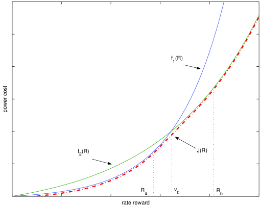
When $w_{1}<w_{2}$, Lemma 1 asserts that if $\frac{\mu_{1}}{w_{1}h_{1}}\geq\frac{\mu_{2}}{w_{2}h_{2}}$, the C$\thicksim$R curve $f_{1}(x)$ of user 1 stays always above $f_{2}(x)$. If $\frac{\mu_{1}}{w_{1}h_{1}}<\frac{\mu_{2}}{w_{2}h_{2}}$, the two C$\thicksim$R curves cross each other once at $v_{0}$, as shown in Fig. 1; hence, $\forall x\in(0,v_{0})$, we have $f_{2}(x)>f_{1}(x)$; and for $x>v_{0}$, $f_{2}(x)<f_{1}(x)$. Using Lemma 1, we can characterize $J(R(\mathbf{h}))$ in (8) as follows.

Lemma 2

For $K=2$ and $w_{1}<w_{2}$, the solution to (8) is:

1. If $\frac{\mu_{1}}{w_{1}h_{1}}\geq\frac{\mu_{2}}{w_{2}h_{2}}$, then $J(R(\mathbf{h}))=f_{2}(R(\mathbf{h}))$, which is achieved by the allocation $\tau_{1}^{*}(\mathbf{h})=0$, $r_{1}^{*}(\mathbf{h})=0$, $\tau_{2}^{*}(\mathbf{h})=1$, and $r_{2}^{*}(\mathbf{h})=R(\mathbf{h})/w_{2}$.

2. If $\frac{\mu_{1}}{w_{1}h_{1}}<\frac{\mu_{2}}{w_{2}h_{2}}$, then

   $$J(R(\mathbf{h}))=\begin{cases}f_{1}(R(\mathbf{h})),&\mbox{if}\;\;0<R(\mathbf{h})\leq R_{a}(\mathbf{h});\\ f_{2}(R(\mathbf{h})),&\mbox{if}\;\;R(\mathbf{h})\geq R_{b}(\mathbf{h});\\ f_{1}(R_{a}(\mathbf{h}))+s_{0}(\mathbf{h})[R(\mathbf{h})-R_{a}(\mathbf{h})],&\mbox{if}\;\;R_{a}(\mathbf{h})<R<R_{b}(\mathbf{h});\end{cases}$$ (11)

   where

   $$R_{a}(\mathbf{h})=w_{1}\log\left(\frac{s_{0}(\mathbf{h})w_{1}h_{1}}{\ln 2\mu_{1}}\right)>0,\quad\quad R_{b}(\mathbf{h})=w_{2}\log\left(\frac{s_{0}(\mathbf{h})w_{2}h_{2}}{\ln 2\mu_{2}}\right)>0,$$ (12)

   and $s_{0}(\mathbf{h})$ is the solution of the equation

   $$g(x,\mathbf{h}):=x\left(w_{2}\log\left(\frac{xw_{2}h_{2}}{\ln 2\mu_{2}}\right)-w_{1}\log\left(\frac{xw_{1}h_{1}}{\ln 2\mu_{1}}\right)-\frac{w_{2}-w_{1}}{\ln 2}\right)+\frac{\mu_{2}}{h_{2}}-\frac{\mu_{1}}{h_{1}}=0,$$ (13)

   i.e., $g(s_{0}(\mathbf{h}),\mathbf{h})=0$. The minimum cost $J(R(\mathbf{h}))$ is then achieved with these policies:

   1. if $0<R(\mathbf{h})\leq R_{a}(\mathbf{h})$, then

      $$\begin{cases}\tau_{1}^{*}(\mathbf{h})=1,&r_{1}^{*}(\mathbf{h})=R(\mathbf{h})/w_{1},\\ \tau_{2}^{*}(\mathbf{h})=0,&r_{2}^{*}(\mathbf{h})=0;\end{cases}$$ (14)

   2. if $R(\mathbf{h})\geq R_{b}(\mathbf{h})$, then

      $$\begin{cases}\tau_{1}^{*}(\mathbf{h})=0,&r_{1}^{*}(\mathbf{h})=0,\\ \tau_{2}^{*}(\mathbf{h})=1,&r_{2}^{*}(\mathbf{h})=R(\mathbf{h})/w_{2};\end{cases}$$ (15)

   3. if $R_{a}(\mathbf{h})<R(\mathbf{h})<R_{b}(\mathbf{h})$, then

      $$\begin{cases}\tau_{1}^{*}(\mathbf{h})=\frac{R(\mathbf{h})-R_{a}(\mathbf{h})}{R_{b}(\mathbf{h})-R_{a}(\mathbf{h})},&r_{1}^{*}(\mathbf{h})=R_{a}(\mathbf{h})/w_{1},\\ \tau_{2}^{*}(\mathbf{h})=1-\tau_{1}(\mathbf{h}),&r_{2}^{*}(\mathbf{h})=R_{b}(\mathbf{h})/w_{2}.\end{cases}$$ (16)

Proof: See Appendix A2. $\Box$

Lemma 2 specifies the optimal power cost curve $J(R(\mathbf{h}))$ for each fading state $\mathbf{h}$ when $w_{1}<w_{2}$. Specifically, if $\frac{\mu_{1}}{w_{1}h_{1}}\geq\frac{\mu_{2}}{w_{2}h_{2}}$, $J(R(\mathbf{h}))$ is simply $f_{2}(R(\mathbf{h}))$; otherwise, $J(R(\mathbf{h}))$ comprises part of the $f_{1}(R(\mathbf{h}))$ curve, the tangent line, and part of the $f_{2}(R(\mathbf{h}))$ curve, as indicated in Fig. 1. Having obtained $J(R(\mathbf{h}))$, we now solve (9) to obtain the optimal resource allocation policies.

Theorem 1

For $K=2$ and $w_{1}<w_{2}$, the optimal rate and time allocation policies with respect to the minimization problem (4) are as follows:

1. If $\frac{\mu_{1}}{w_{1}h_{1}}\geq\frac{\mu_{2}}{w_{2}h_{2}}$, then

   $$\begin{cases}\tau_{1}^{*}(\mathbf{h})=0,&r_{1}^{*}(\mathbf{h})=0,\\ \tau_{2}^{*}(\mathbf{h})=1,&r_{2}^{*}(\mathbf{h})=\left[\log\lambda^{*}-\log\left(\frac{\ln 2\mu_{2}}{w_{2}h_{2}}\right)\right]_{+}.\end{cases}$$ (17)

2. If $\frac{\mu_{1}}{w_{1}h_{1}}<\frac{\mu_{2}}{w_{2}h_{2}}$, and $\xi:=\left(\frac{((w_{1}h_{1})/(\ln 2\mu_{1}))^{w_{1}}}{((w_{2}h_{2})/(\ln 2\mu_{2}))^{w_{2}}}\right)^{\frac{1}{w_{2}-w_{1}}}$,

   1. if $\lambda^{*}\leq\xi$ or if $\lambda^{*}>\xi$ and $g(\lambda^{*},\mathbf{h})<0$, then

      $$\begin{cases}\tau_{1}^{*}(\mathbf{h})=1,&r_{1}^{*}(\mathbf{h})=\left[\log\lambda^{*}-\log\left(\frac{\ln 2\mu_{1}}{w_{1}h_{1}}\right)\right]_{+},\\ \tau_{2}^{*}(\mathbf{h})=0,&r_{2}^{*}(\mathbf{h})=0;\end{cases}$$ (18)

   2. if $\lambda^{*}>\xi$ and $g(\lambda^{*},\mathbf{h})>0$, then

      $$\begin{cases}\tau_{1}^{*}(\mathbf{h})=0,&r_{1}^{*}(\mathbf{h})=0,\\ \tau_{2}^{*}(\mathbf{h})=1,&r_{2}^{*}(\mathbf{h})=\left[\log\lambda^{*}-\log\left(\frac{\ln 2\mu_{2}}{w_{2}h_{2}}\right)\right]_{+};\end{cases}$$ (19)

   3. if $\lambda^{*}>\xi$ and $g(\lambda^{*},\mathbf{h})=0$, then for an arbitrary $\tau_{0}^{*}\in[0,1]$,

      $$\begin{cases}\tau_{1}^{*}(\mathbf{h})=\tau_{0}^{*},&r_{1}^{*}(\mathbf{h})=\left[\log\lambda^{*}-\log\left(\frac{\ln 2\mu_{1}}{w_{1}h_{1}}\right)\right]_{+},\\ \tau_{2}^{*}(\mathbf{h})=1-\tau_{0}^{*},&r_{2}^{*}(\mathbf{h})=\left[\log\lambda^{*}-\log\left(\frac{\ln 2\mu_{2}}{w_{2}h_{2}}\right)\right]_{+}.\end{cases}$$ (20)

Function $g(x,\mathbf{h})$ is given by (13), and $\lambda^{*}$, $\tau_{0}^{*}$ are obtained numerically by satisfying the weighted sum-rate constraint $E_{\mathbf{h}}[\sum_{k=1}^{2}w_{k}\tau_{k}^{*}(\mathbf{h})r_{k}^{*}(\mathbf{h})]=\bar{R}$.

Proof: See Appendix B. $\Box$

Note that depending on $\lambda^{*}$, water-filling in (17)-(20) may result in zero transmission rate for the user which has been assigned the entire or part of the block. Therefore, for some fading states where the channel is really bad, both users should defer. Comparing (8) and (9) with [11, eqs. (11), (13)], we find that our power minimization yields similar “opportunistic” policies as the rate maximization in [11].

Since $\tau_{0}^{*}$ can take any arbitrary value between 0 and 1, the solution in (20) is not unique. However, under the assumption of continuous joint fading distribution density, the probability of $g(\lambda^{*},\mathbf{h})=0$ is zero, and therefore case c) is an event of measure zero. Thus, after setting $\tau_{0}^{*}$ to an arbitrary value in [0,1], $\lambda^{*}$ can be uniquely determined by an one-dimensional, e.g., bi-sectional, search. From Theorem 1, it is clear that in order to achieve energy efficiency over TDMA fading channels, most of the time we should allow one user to transmit per block. This also holds true in rate maximization for TDMA fading channels [11], even though the resultant time and rate allocation fractions are different.

To extend our two-user results to $K>2$ users, we will need definition of the convex envelope.

Definition 2

The convex envelope $f^{c}(x)$ of a function $f(x)$ is the solution to the optimization problem

$$f^{c}(x)=\max_{a,b}\;\;ax+b,\quad\quad\mbox{subject to}\quad ax+b\leq f(x),\;\forall x.$$ (21)

Namely, $f^{c}(x)$ is the boundary surface of the convex hull of the function’s epigraph [16].

Using the definition $\bar{f}(x):=\min_{1\leq k\leq K}f_{k}(x)$, we can verify the following property:

Proposition 1

The optimal C$\thicksim$R function $J(R(\mathbf{h}))$ in (8) is the convex envelope of $\bar{f}(R(\mathbf{h}))$ in the two-user case; i.e., $J(R(\mathbf{h}))=\bar{f}^{c}(R(\mathbf{h}))$ as determined by Lemma 2 and Definition 2.

Proof: If $w_{1}<w_{2}$ and $\frac{\mu_{1}}{w_{1}h_{1}}\geq\frac{\mu_{2}}{w_{2}h_{2}}$, then $J(R(\mathbf{h}))=f_{2}(R(\mathbf{h}))=\bar{f}(R(\mathbf{h}))$. It is trivial to show $J(R(\mathbf{h}))=\bar{f}^{c}(R(\mathbf{h}))$. If $w_{1}<w_{2}$ and $\frac{\mu_{1}}{w_{1}h_{1}}<\frac{\mu_{2}}{w_{2}h_{2}}$, then it is easy to show that $J(R(\mathbf{h}))$ is convex since it has non-decreasing first derivatives for all $R(\mathbf{h})\geq 0$. If the convex envelope $\bar{f}^{c}(R(\mathbf{h}))$ were not given by $J(R(\mathbf{h}))$, then $\bar{f}^{c}(R(\mathbf{h}))$ would be strictly greater than $J(R(\mathbf{h}))$ for some $R(\mathbf{h})$. Since the first and the third branches of $J(R(\mathbf{h}))$ in (11) are exactly $\bar{f}(R(\mathbf{h}))$, for $0<R(\mathbf{h})\leq R_{a}(\mathbf{h})$ and $R(\mathbf{h})\geq R_{b}(\mathbf{h})$, we must have $\bar{f}^{c}(R(\mathbf{h}))=J(R(\mathbf{h}))$. Therefore, $\bar{f}^{c}(R(\mathbf{h}))$ can only be greater than $J(R(\mathbf{h}))$ for $R(\mathbf{h})\in(R_{a}(\mathbf{h}),R_{b}(\mathbf{h}))$. But since $\bar{f}^{c}(R(\mathbf{h}))$ is convex, Jensen’s inequality implies that its value for any $R_{a}(\mathbf{h})<R(\mathbf{h})<R_{b}(\mathbf{h})$ can not be greater than the value given by the line segment connecting $\bar{f}(R_{a}(\mathbf{h}))$ with $\bar{f}(R_{b}(\mathbf{h}))$. This leads to a contradiction, and thus $J(R(\mathbf{h}))=\bar{f}^{c}(R(\mathbf{h}))$. $\Box$

III-A2 $K$-Use Case

Generalizing Proposition 1 to $K>2$ users, we can show that:

Theorem 2

For a $K$-user TDMA block fading channel, the optimal C$\thicksim$R function $J(R(\mathbf{h}))$ at each fading state $\mathbf{h}$ is the convex envelope of $\bar{f}(R(\mathbf{h})):=\min_{1\leq k\leq K}f_{k}(R(\mathbf{h}))$, and the optimality is achieved by allowing at most two users to transmit per time block.

Proof: See Appendix C. $\Box$

Although Theorem 2 asserts achievability of the optimal policies, it does not provide algorithms realizing these optimal allocation strategies. The latter are challenging since obtaining convex envelopes is generally difficult. As pointed out in [17], the rate-maximizing resource allocation for TD broadcast fading channels in [11] is obtained by water-filling across realizations of concave envelopes. Our energy-efficient resource allocation policies under a weighted sum average rate constraint for TDMA fading channels are obtained via water-filling across realizations of the convex envelopes $J(R(\mathbf{h}))$. But in order to determine $J(R(\mathbf{h}))$, we must generalize Lemma 2 to the $K$-user case. This is accomplished with the following algorithm.

Algorithm 1

initialization: Let $\mathbf{u}:=[u_{1},\ldots,u_{K_{0}}]^{T}$ (initially set equal to the empty set $\phi$) denote the set of active users during a given block, $\mathbf{s}:=[s_{1},\ldots,s_{K_{0}}]^{T}$ the set of slopes of (possibly multiple) tangent lines common to the active C$\thicksim$R curves (also initially set to $\phi$), and let the iteration index be $m=1$.

1. Remove the C$\thicksim$R function of user $k$ from $J(R(\mathbf{h}))$ if $\exists i\neq k$ such that $w_{k}\leq w_{i}$ and $\frac{\mu_{k}}{w_{k}h_{k}}\geq\frac{\mu_{i}}{w_{i}h_{i}}$, because in this case $\forall x>0$, $f_{k}(x)<f_{i}(x)$ and $f_{k}(x)$ will not appear in the expression of $J(R(\mathbf{h}))$ for the reasons we detailed in Lemma 2. Let $K_{r}$ be the number of users remaining after such a successive elimination of their C$\thicksim$R functions from $J(R(\mathbf{h}))$, and define the permutation $\pi(\cdot)$ such that $w_{\pi(1)}<w_{\pi(2)}<\cdots<w_{\pi(K_{r})}$. Then through successive pairwise comparisons and user C$\thicksim$R function removals, we can ensure that $\frac{\mu_{\pi(1)}}{w_{\pi(1)}h_{\pi(1)}}<\frac{\mu_{\pi(2)}}{w_{\pi(2)}h_{\pi(2)}}<\cdots<\frac{\mu_{\pi(K_{r})}}{w_{\pi(K_{r})}h_{\pi(K_{r})}}$.

2. Let the $m$th element of $\mathbf{u}$ be $u_{m}=\pi(1)$. If $K_{r}\geq 2$, go to Step 3. If $K_{r}<2$, all users with C$\thicksim$R functions not appearing in $J(R(\mathbf{h}))$ have been removed. Then set the number of active users be $K_{0}=m$, $s_{m}=\infty$, and stop.

3. For $1\leq i\leq K_{r}-1$, define

   $$g_{i}(x,\mathbf{h}) := x\left(w_{\pi(i+1)}\log\left(\frac{xw_{\pi(i+1)}h_{\pi(i+1)}}{\ln 2\mu_{\pi(i+1)}}\right)-w_{\pi(1)}\log\left(\frac{xw_{\pi(1)}h_{\pi(1)}}{\ln 2\mu_{\pi(1)}}\right)\right)$$ (22)

   $$-x\left(\frac{w_{\pi(i+1)}-w_{\pi(1)}}{\ln 2}\right)+\frac{\mu_{\pi(i+1)}}{h_{\pi(i+1)}}-\frac{\mu_{\pi(1)}}{h_{\pi(1)}},$$

   and find the $\xi_{i}$ satisfying $g_{i}(\xi_{i},\mathbf{h})=0$, $\log\left(\frac{xw_{\pi(i+1)}h_{\pi(i+1)}}{\ln 2\mu_{\pi(i+1)}}\right)>0$ and $\log\left(\frac{xw_{\pi(1)}h_{\pi(1)}}{\ln 2\mu_{\pi(1)}}\right)>0$. Let also $s_{m}=\min_{i}\{\xi_{i}\}$, and $i^{*}=\arg\;\min_{i}\{\xi_{i}\}$. Remove C$\thicksim$R functions of users $\pi(k)$ for which $1\leq k\leq i^{*}$. Increase $m$ by 1 and return to S1).

Using Algorithm 1, we obtain $\mathbf{u}$ and $\mathbf{s}$. If $K_{0}=1$, $J(R(\mathbf{h}))$ is simply $f_{u_{1}}(\cdot)$; if $K_{0}>1$, then $J(R(\mathbf{h}))$ comprises pieces of the curves $\left\{f_{u_{m}}(\cdot)\right\}_{m=1}^{K_{0}}$ as well as the common tangent line segments between $f_{u_{m}}(\cdot)$ and $f_{u_{m+1}}(\cdot)$, $1\leq m\leq K_{0}-1$, the slopes of which are $\left\{s_{m}\right\}_{m=1}^{K_{0}-1}$. By denoting $R_{a_{0}}(\mathbf{h})=R_{b_{0}}(\mathbf{h})=0$, $R_{a_{K_{0}}}(\mathbf{h})=R_{b_{K_{0}}}(\mathbf{h})=\infty$, and letting $R_{a_{m}}(\mathbf{h})$ and $R_{b_{m}}(\mathbf{h})$ be the points with equal first derivatives $f_{u_{m}}^{(1)}(R_{a_{m}}(\mathbf{h}))=f_{u_{m+1}}^{(1)}(R_{b_{m}}(\mathbf{h}))=s_{m}$, we can write

$$J(R(\mathbf{h}))=\begin{cases}f_{u_{m}}(R(\mathbf{h})),&\mbox{if}\;\;R_{b_{m-1}}(\mathbf{h})\leq R(\mathbf{h})\leq R_{a_{m}}(\mathbf{h});\\ f_{u_{m}}(R_{a_{m}}(\mathbf{h}))+s_{m}[R(\mathbf{h})-R_{a_{m}}(\mathbf{h})],&\mbox{if}\;\;R_{a_{m}}(\mathbf{h})\leq R<R_{b_{m}}(\mathbf{h}).\end{cases}$$ (23)

Arguing as in the proof of Proposition 1, it follows readily that $J(R(\mathbf{h}))$ is the convex envelope of $\bar{f}(R(\mathbf{h}))$. Once having $J(R(\mathbf{h}))$, we will implement a water-filling strategy to obtain the energy-efficient resource allocation across realizations of $\mathbf{h}$. First, for any user $k\notin\mathbf{u}$, we let $\tau_{k}^{*}(\mathbf{h})=0$ and $r_{k}^{*}(\mathbf{h})=0$. The rate and time allocation for the remaining $K_{0}$ users is given as follows.

Algorithm 2

1. If $K_{0}=1$, then

   $$\tau_{u_{1}}^{*}(\mathbf{h})=1,\quad\quad r_{u_{1}}^{*}(\mathbf{h})=\left[\log\lambda^{*}-\log\left(\frac{\ln 2\mu_{u_{1}}}{w_{u_{1}}h_{u_{1}}}\right)\right]_{+}.$$ (24)

2. If $K_{0}>1$, set $s_{0}=0$. Since $0=s_{0}<s_{1}<\cdots<s_{K_{0}}=\infty$, for the given $\lambda^{*}$, there exists $j\in\{1,2,\ldots,K_{0}\}$ such that $s_{j-1}<\lambda^{*}<s_{j}$ or $\lambda^{*}=s_{j}$.

   1. If $\exists j$ such that $s_{j-1}<\lambda^{*}<s_{j}$, we know $J(R(\mathbf{h}))=f_{u_{j}}(R(\mathbf{h}))$. In this case, we set

      $$\tau_{u_{j}}^{*}(\mathbf{h})=1,\quad\quad r_{u_{j}}^{*}(\mathbf{h})=\left[\log\lambda^{*}-\log\left(\frac{\ln 2\mu_{u_{j}}}{w_{u_{j}}h_{u_{j}}}\right)\right]_{+};$$ (25)

      and $\forall i\neq j$, $\tau_{u_{i}}^{*}(\mathbf{h})=0$ and $r_{u_{i}}^{*}(\mathbf{h})=0$.

   2. If $\exists j$ such that $\lambda^{*}=s_{j}$, then $J(R(\mathbf{h}))=f_{u_{j}}(R_{a_{j}}(\mathbf{h}))+s_{j}[R(\mathbf{h})-R_{a_{j}}(\mathbf{h})]$. As in the two-user case, we set

      $$\begin{cases}\tau_{u_{j}}^{*}(\mathbf{h})=\tau_{0}^{*},&r_{u_{j}}^{*}(\mathbf{h})=\left[\log\lambda^{*}-\log\left(\frac{\ln 2\mu_{u_{j}}}{w_{u_{j}}h_{u_{j}}}\right)\right]_{+},\\ \tau_{u_{j+1}}^{*}(\mathbf{h})=1-\tau_{0}^{*},&r_{u_{j+1}}^{*}(\mathbf{h})=\left[\log\lambda^{*}-\log\left(\frac{\ln 2\mu_{u_{j+1}}}{w_{u_{j+1}}h_{u_{j+1}}}\right)\right]_{+};\end{cases}$$ (26)

      and $\forall i\neq j,j+1$, $\tau_{u_{i}}^{*}(\mathbf{h})=0$ and $r_{u_{i}}^{*}(\mathbf{h})=0$.

In eqs. (24)-(26), $\lambda^{*}$ and $\tau_{0}^{*}$ are chosen to satisfy the weighted sum-rate constraint

$$E_{\mathbf{h}}\left[\sum_{k=1}^{K}w_{k}\tau_{k}^{*}(\mathbf{h})r_{k}^{*}(\mathbf{h})\right]=\bar{R}.$$ (27)

Under the assumption of continuous joint fading distribution density, the value of $\tau_{0}^{*}$ does not affect the weighted sum-rate constraint, and $\lambda^{*}$ can be uniquely determined by an one-dimensional search, as in the two-user case. To achieve energy efficiency, we should only allow at most two users (and most of the time only one user) to transmit per time block in the $K$-user case. Again in (24)-(26), water-filling may result in zero transmission rate for the user which has been assigned the entire or part of the time block. For some fading states, when all channels are in deep fading, all users should defer. Also note that Algorithms 1 and 2 are dual to those in [11] for power minimization under an average sum-rate constraint.

III-B Quantized CSI and Finite AMC Modes

In this section, we provide a novel formulation and solve the energy minimization problem under a weighted sum average rate constraint for the finite-AMC-mode case. In practice, a user may not be able to support an infinite number of codebooks. Moreover, the codewords in use may not be capacity-achieving. It is thus worth investigating energy-efficient resource allocation for practical systems where each user can only support a finite number of AMC modes. Notice that since transmitters can transmit with a finite number of AMC modes, only quantized CSI could be fed back from the access point to the transmitters suffices.

For user $k\in[1,K]$, an AMC mode corresponds to a rate-power pair $(\rho_{k,l},p_{k,l})$, $l=1,\ldots,M_{k}$, where $M_{k}$ denotes the number of AMC modes. A pair $(\rho_{k,l},p_{k,l})$ indicates that for transmission rate $\rho_{k,l}$ provided by the $l$th AMC mode, the minimum received power required is $p_{k,l}$. Notice that the minimum power $p_{k,l}$ may not be given by $2^{\rho_{k,l}}-1$ as in the capacity-achieving case, and some extra power may be required in practice. Also, the rate $\rho_{k,l}$ is maintained with a prescribed symbol error probability (SEP), and $p_{k,l}$ is the corresponding minimum received power under the SEP constraint. For this reason, we need to implicitly include the SEP constraints in our optimization. Although the $k$th user only supports $M_{k}$ AMC modes, this user can still support through time-sharing continuous rates up to a maximum value determined by the highest-rate AMC mode $\rho_{k,M_{k}}$.

By setting $\rho_{k,0}=0$ and $p_{k,0}=0$ and letting $\gamma_{k,l}:=(p_{k,l}-p_{k,l-1})/(\rho_{k,l}-\rho_{k,l-1})$, we define the piece-wise linear function relating transmit power with rate as

$$\Upsilon_{k}(r_{k}(\mathbf{h}))=\begin{cases}p_{k,l-1}/h_{k}+\gamma_{k,l}(r_{k}(\mathbf{h})-\rho_{k,l-1})/h_{k},&\rho_{k,l-1}\leq r_{k}(\mathbf{h})\leq\rho_{k,l},\;\;l\in[1,M_{k}];\\ \infty,&r_{k}(\mathbf{h})>\rho_{k,M_{k}}.\end{cases}$$ (28)

Notice that in order to support rate $\rho_{k,l}$ with channel coefficient $h_{k}$, the required transmit power is scaled as $p_{k,l}/h_{k}$. For practical modulation-coding schemes with e.g., $M$-QAM constellations and error-control codes, $\Upsilon_{k}(r_{k}(\mathbf{h}))$ is guaranteed to be convex [2]. Using (28) to replace the power-rate relationship implied by Shannon’s capacity formula, we can define a power region as [c.f. (2), (3)]

$${\cal P}^{\prime}(\bar{R})=\bigcup_{(\mathbf{r}(\cdot),\boldsymbol{\tau}(\cdot))\in{\cal F}_{\mathbf{w}}}{\cal P}_{TD}^{\prime}(\mathbf{r}(\cdot),\boldsymbol{\tau}(\cdot)),$$ (29)

where

$${\cal P}_{TD}^{\prime}(\mathbf{r}(\cdot),\boldsymbol{\tau}(\cdot))=\left\{\mathbf{\bar{p}}:\bar{P}_{k}\geq E_{\mathbf{h}}\left[\tau_{k}(\mathbf{h})\Upsilon_{k}(r_{k}(\mathbf{h}))\right],\quad\quad 1\leq k\leq K\right\}.$$ (30)

It is easy to show that the $K$-dimensional ${\cal P}^{\prime}(\bar{R})$ is feasible and convex. The optimization problem thus becomes

$$\min_{\mathbf{\bar{p}}}\boldsymbol{\mu}^{T}\mathbf{\bar{p}},\quad\quad\mbox{subject to}\quad\mathbf{\bar{p}}\in{\cal P}^{\prime}(\bar{R}).$$ (31)

We can rewrite (31) as

$$\begin{cases}\min_{\mathbf{r}(\cdot),\boldsymbol{\tau}(\cdot)}E_{\mathbf{h}}\left[\sum_{k=1}^{K}\mu_{k}\tau_{k}(\mathbf{h})\Upsilon_{k}(r_{k}(\mathbf{h}))\right]\\ \mbox{subject to}\quad E_{\mathbf{h}}\left[\sum_{k=1}^{K}w_{k}\tau_{k}(\mathbf{h})r_{k}(\mathbf{h})\right]=\bar{R},\quad\quad\forall\mathbf{h}\;\;\sum_{k=1}^{K}\tau_{k}(\mathbf{h})=1.\end{cases}$$ (32)

As in the infinite-codebook case, we can still decompose (32) into two sub-problems. That is, we first optimize per fading realization, and then apply water-filling across $J(R(\mathbf{h}))$ realizations to obtain the optimal resource allocation policies.

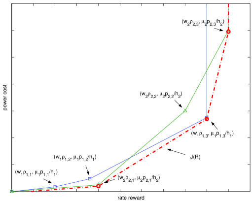
Recalling the weighted rate-reward $R_{k}(\mathbf{h})=w_{k}r_{k}(\mathbf{h})$, the C$\thicksim$R function corresponding to the $k$th user is now $f_{k}(R_{k}(\mathbf{h})):=\mu_{k}\Upsilon_{k}(R_{k}(\mathbf{h})/w_{k})$ which is a piece-wise linear curve through the points $\{(w_{k}\rho_{k,l},\mu_{k}p_{k,l}/h_{k})\}_{l=1}^{M_{k}}$. Since the C$\thicksim$R functions are piece-wise linear, the convex envelope $J(R(\mathbf{h}))$ of their $\min_{k}\;f_{k}(R(\mathbf{h}))$ can be obtained by simply comparing the slopes of a finite number of straight line segments. To this end, we implement the following algorithm:

Algorithm 3

initialization: Define the set of points $\bar{\mathbf{m}}_{k}:=[(w_{k}\rho_{k,l},\mu_{k}p_{k,l}/h_{k}),\;\;l=1,\ldots,M_{k}]^{T}$, $\forall k\in[1,K]$. Start with the set of slopes $\mathbf{s}:=[s_{0},\ldots,s_{m-1}]^{T}$, set of rate rewards $\mathbf{r}:=[R_{0},\ldots,R_{m-1}]^{T}$, set of power costs $\mathbf{c}:=[C_{0},\ldots,C_{m-1}]^{T}$ with $s_{0}=R_{0}=C_{0}=0$, and let the iteration index be $m=1$.

1. Consider the point $(x_{0},y_{0})=(R_{m-1},C_{m-1})$. For $k=1,\ldots,K$, if $\bar{\mathbf{m}}_{k}\neq\phi$, let the $i$th element in $\bar{\mathbf{m}}_{k}$ be $(w_{k}\rho_{k,\bar{\mathbf{m}}_{k}(i)},\mu_{k}p_{k,\bar{\mathbf{m}}_{k}(i)}/h_{k})$. Also, set $(x_{k},y_{k})=\left(w_{k}\rho_{k,\bar{\mathbf{m}}_{k}(1)},p_{k,\bar{\mathbf{m}}_{k}(1)}/h_{k}\right)$.

2. Let $s_{m}=\min_{k:\;\bar{\mathbf{m}}_{k}\neq\phi}\;\frac{y_{k}-y_{0}}{x_{k}-x_{0}}$ and $k^{*}=\arg\;\min_{k:\;\bar{\mathbf{m}}_{k}\neq\phi}\;\frac{y_{k}-y_{0}}{x_{k}-x_{0}}$. Set $R_{m}=x_{k^{*}}$ and $C_{m}=y_{k^{*}}$.

   1. For each $k\neq k^{*}$ and $\bar{\mathbf{m}}_{k}\neq\phi$, $k\in[1,K]$, let $i^{*}=\max_{i}\;\{i:w_{k}\rho_{k,\bar{\mathbf{m}}_{k}(i)}\leq w_{k^{*}}\rho_{k^{*},\bar{\mathbf{m}}_{k^{*}}(1)}\}$. If $i^{*}\neq 0$, then remove all $(w_{k}\rho_{k,\bar{\mathbf{m}}_{k}(i)},\mu_{k}p_{k,\bar{\mathbf{m}}_{k}(i)}/h_{k})$, $i\in[1,i^{*}]$, from $\bar{\mathbf{m}}_{k}$, and reduce $M_{k}$ by $i^{*}$. Note that in the next iteration, the original $(w_{k}\rho_{k,\bar{\mathbf{m}}_{k}(i^{*}+1)},$ $\mu_{k}p_{k,\bar{\mathbf{m}}_{k}(i^{*}+1)}/h_{k})$ becomes the first element $(w_{k}\rho_{k,\bar{\mathbf{m}}_{k}(1)},\mu_{k}q_{k,\bar{\mathbf{m}}_{k}(1)}/h_{k})$ of $\bar{\mathbf{m}}_{k}$.

   2. Remove $(w_{k^{*}}\rho_{k^{*},\bar{\mathbf{m}}_{k^{*}}(1)},\mu_{k^{*}}p_{k^{*},\bar{\mathbf{m}}_{k^{*}}(1)}/h_{k^{*}})$ from $\bar{\mathbf{m}}_{k^{*}}$ and reduce $M_{k^{*}}$ by 1.

   If $\bar{\mathbf{m}}_{k}=\phi$ (i.e., $M_{k}=0$), $\forall k\in[1,K]$, set $K_{0}=m$ and stop. Otherwise, increase $m$ by 1 and go to S1). Notice that $K_{0}$ is the number of corner points of the wanted convex envelope $J(R(\mathbf{h}))$.

Having obtained $\mathbf{s}$, $\mathbf{r}$ and $\mathbf{c}$, we can express $J(R(\mathbf{h}))$ as

$$J(R(\mathbf{h}))=\begin{cases}C_{m-1}+s_{m}(R(\mathbf{h})-R_{m}),&R_{m-1}\leq R(\mathbf{h})\leq R_{m},\;\;m\in[1,K_{0}];\\ \infty,&R(\mathbf{h})>R_{K_{0}}.\end{cases}$$ (33)

An illustration example for Algorithm 3 and the resultant $J(R(\mathbf{h}))$ is shown in Fig. 2, where each of the two users can support three AMC modes. In S1 of Algorithm 3, we first compare the slopes $\mu_{1}p_{1,1}/(h_{1}w_{1}\rho_{1,1})$ and $\mu_{2}p_{2,1}/(h_{2}w_{2}\rho_{2,1})$ and find $\mu_{2}p_{2,1}/(h_{2}w_{2}\rho_{2,1})<\mu_{1}p_{1,1}/(h_{1}w_{1}\rho_{1,1})$. Therefore, we let $R_{1}=w_{2}\rho_{2,1}$ and $C_{1}=\mu_{2}p_{2,1}/h_{2}$. Since both $w_{1}\rho_{1,1}$ and $w_{1}\rho_{1,2}$ are less than $w_{2}\rho_{2,1}$, we remove the first two AMC modes of user 1 from $\bar{\mathbf{m}}_{1}$ in S2 a); whereas we remove the first AMC mode of user 2 from $\bar{\mathbf{m}}_{2}$ in S2 b). In S1 of the next iteration, we compare the slope between points $(w_{1}\rho_{1,3},\mu_{1}p_{1,3}/h_{1})$ and $(w_{2}\rho_{2,1},\mu_{2}p_{2,1}/h_{2})$, with the slope between points $(w_{2}\rho_{2,2},\mu_{2}p_{2,2}/h_{2})$ and $(w_{2}\rho_{2,1},\mu_{2}p_{2,1}/h_{2})$. In this case, we should set $R_{2}=w_{1}\rho_{1,3}$ and $C_{2}=\mu_{1}p_{1,3}/h_{1}$. In S2, we remove $(w_{2}\rho_{2,2},\mu_{2}p_{2,2}/h_{2})$ from $\bar{\mathbf{m}}_{2}$, and remove $(w_{1}\rho_{1,3},\mu_{1}p_{1,3}/h_{1})$ from $\bar{\mathbf{m}}_{1}$. In the last iteration, we obtain $R_{3}=w_{2}\rho_{2,3}$ and $C_{3}=\mu_{2}p_{2,3}/h_{2}$, and $J(R(\mathbf{h}))$ is determined.

Having determined $J(R(\mathbf{h}))$ as in (33), we implement water-filling across realizations of $J(R(\mathbf{h}))$ to derive the optimal resource allocation policies. Different from the infinite-codebook case where all $J(R(\mathbf{h}))$ have continuous slopes, here $J(R(\mathbf{h}))$ are piecewise-linear. Therefore, water-filling should take into account the finite number of slopes of $J(R(\mathbf{h}))$. A somewhat related problem was dealt with in [12], where water-filling over some piecewise-linear concave functions was used to determine the boundary surface of the outage probability region. But energy-efficient resource allocation policies for finite-AMC-modes were not considered in [11] and [12].

Recall that $K_{0}$ and all entries of $\mathbf{s}$, $\mathbf{r}$ and $\mathbf{c}$ are functions of $\mathbf{h}$. Since every point of the convex envelope $J(R(\mathbf{h}))$ can be achieved by time-sharing between points $(R_{m}(\mathbf{h}),C_{m}(\mathbf{h}))$, finding the optimal resource allocation strategies is equivalent to solving the following minimization problem:

$$\begin{cases}\min_{\mathbf{\tilde{\tau}}(\mathbf{h})}\;E_{\mathbf{h}}\left[\sum_{m=1}^{K_{0}}\tilde{\tau}_{m}(\mathbf{h})C_{m}(\mathbf{h})\right]\\ \mbox{subject to}\quad\quad E_{\mathbf{h}}\left[\sum_{m=1}^{K_{0}}\tilde{\tau}_{m}(\mathbf{h})R_{m}(\mathbf{h})\right]\geq\bar{R},\quad\sum_{m=1}^{K_{0}}\tilde{\tau}_{m}(\mathbf{h})=1.\end{cases}$$ (34)

Theorem 3

If the optimization (34) is feasible, by setting $s_{K_{0}+1}(\mathbf{h})=\infty$, then $\forall\mathbf{h}$, we have the optimal solution $\left\{\tilde{\tau}_{m}^{*}(\mathbf{h})\right\}_{m=1}^{K_{0}}$, and thus the optimal allocation policies $\tau_{k}^{*}(\mathbf{h})$ and $r_{k}^{*}(\mathbf{h})$ ($1\leq k\leq K$) for the original problem (31) as follows:

1. If $\lambda^{*}<s_{1}(\mathbf{h})$, then $\tilde{\tau}_{m}^{*}(\mathbf{h})=0$, $\forall m=1,\ldots,K_{0}$; consequently, $\tau_{k}^{*}(\mathbf{h})=0$ and $r_{k}^{*}(\mathbf{h})=0$, $\forall k=1,\ldots,K$.

2. If $\exists m^{*}\in\{1,2,\ldots,K_{0}\}$ so that $s_{m^{*}}(\mathbf{h})<\lambda^{*}<s_{m^{*}+1}(\mathbf{h})$, then $\tilde{\tau}_{m^{*}}^{*}(\mathbf{h})=1$, and $\tilde{\tau}_{m}^{*}(\mathbf{h})=0$, $\forall m\neq m^{*}$, $1\leq m\leq K_{0}$. This implies that if $(R_{m^{*}}(\mathbf{h}),C_{m^{*}}(\mathbf{h}))$ belongs to user $k^{*}$, then

   $$\tau_{k^{*}}^{*}(\mathbf{h})=1,\quad\quad r_{k^{*}}^{*}(\mathbf{h})=R_{m^{*}}(\mathbf{h})/w_{k^{*}};$$ (35)

   and $\tau_{k}^{*}(\mathbf{h})=0$ and $r_{k}^{*}(\mathbf{h})=0$, $\forall k\neq k^{*}$, $1\leq k\leq K$.

3. If $\exists m^{*}\in\{1,2,\ldots,K_{0}\}$ so that $\lambda^{*}=s_{m^{*}}(\mathbf{h})$, then $\tilde{\tau}_{m^{*}}^{*}(\mathbf{h})=\tau_{0}^{*}$, $\tilde{\tau}_{m^{*}-1}^{*}(\mathbf{h})=1-\tau_{0}^{*}$, and $\tilde{\tau}_{m}^{*}(\mathbf{h})=0$, $\forall m\neq m^{*},m^{*}-1$, $1\leq m\leq K_{0}$. This implies that if $(R_{m^{*}}(\mathbf{h}),C_{m^{*}}(\mathbf{h}))$ and $(R_{m^{*}-1}(\mathbf{h}),C_{m^{*}-1}(\mathbf{h}))$ belongs to users $i^{*}$ and $j^{*}$, respectively, then

   $$\begin{cases}\tau_{i^{*}}^{*}(\mathbf{h})=\tau_{0}^{*},&r_{i^{*}}^{*}(\mathbf{h})=R_{m^{*}}(\mathbf{h})/w_{i^{*}},\\ \tau_{j^{*}}^{*}(\mathbf{h})=1-\tau_{0}^{*},&r_{j^{*}}^{*}(\mathbf{h})=R_{m^{*}-1}(\mathbf{h})/w_{j^{*}};\end{cases}$$ (36)

   and $\tau_{k}^{*}(\mathbf{h})=0$ and $r_{k}^{*}(\mathbf{h})=0$, $\forall k\neq i^{*},j^{*}$, $1\leq k\leq K$. Note that if $m^{*}=1$, we let user $i^{*}$ transmit with $\tau_{0}^{*}$ fraction of time and leave the channel idle for the remaining $1-\tau_{0}^{*}$ fraction of time. If $i^{*}=j^{*}$, then we let the same user transmit with two AMC modes, one for $\tau_{0}^{*}$ fraction and the other for $1-\tau_{0}^{*}$ fraction of time.

In eqs. (35) and (36), $\tau_{0}^{*}$ should satisfy the average rate constraint

$$E_{\mathbf{h}}\left[\sum_{k=1}^{K}w_{k}\tau_{k}^{*}(\mathbf{h})r_{k}^{*}(\mathbf{h})\right]=\bar{R}.$$ (37)

Proof: See Appendix D. $\Box$

The results of Theorem 3 are analogous in form with those in [12, Theorem 3], which is a generalization of [13, Lemma 3]. But note that the latter deal with the delay-limited/outage capacity; while our results are for energy-efficient resource allocation using finite-AMC-modes, a subject not considered in [12, 13]. In Theorem 3, $\lambda^{*}$ is the water-filling level. For energy efficiency, we should let the first derivatives $J^{(1)}(R(\mathbf{h}))=\lambda^{*}$. However, since $J(R(\mathbf{h}))$ entails a finite number of slopes, equality can not be always achieved. Thus, our strategy is to select the largest $J^{(1)}(R(\mathbf{h}))\leq\lambda^{*}$. When the largest $J^{(1)}(R(\mathbf{h}))=s_{m^{*}}(\mathbf{h})<\lambda^{*}$, i.e., $s_{m^{*}}(\mathbf{h})<\lambda^{*}<s_{m^{*}+1}(\mathbf{h})$, since the user(s) transmit more efficiently than the required power level, we should allow transmission(s) with peak rate given by $R_{m^{*}}(\mathbf{h})/w_{k^{*}}$. When $\lambda^{*}=s_{m^{*}}(\mathbf{h})$, users transmit as efficiently as required; thus arbitrary time division suffices. When $\lambda^{*}<s_{1}(\mathbf{h})$, no transmission can be carried out as efficiently as required, and all users defer during this fading state. As in the infinite-codebook case, we should allow at most two users to transmit per time block. However, here we also allow one user to transmit in a time-sharing fashion with two AMC modes during some time blocks.

III-C Discrete-Time Allocation

So far we have derived energy-efficient resource allocation strategies under the assumption that the time fraction $\tau_{k}$ assigned to each user can be any real number in [0,1]. In practical TDMA systems, time is usually divided with granularity of one time unit (slot), which is determined by the available bandwidth. Therefore, the transmission time assigned to each user per time block has to be an integer multiple of a “slot”. Take the well-known GSM system as an example [15, Chapter 4]. In each narrowband channel of 200 KHz, time is divided into slots of length 577 $\mu$s and each uplink frame is shared by the users in a time-division manner, and consists of 8 slots. Upon regarding an uplink frame as a frequency flat-fading time block, we can thus only assign each user a time fraction which is an integer multiple of 1/8. However, this extra discrete-time allocation constraint does not affect the derived energy-efficient allocation policies. In our policies, most of the time we should assign the entire time block to a single user. When we occasionally allow two users to transmit (or allow one user to transmit with two AMC modes), the time division between them can be arbitrary. Therefore, our energy-efficient policies can be easily adopted by practical systems which only allow discrete-time allocation among users.

IV Average Individual-Rate Constraints

In resource allocation for multi-access channels, other than a weighted average sum-rate constraint, a more general setting is when each user has an individual average rate requirement. We next consider power minimization under such individual rate constraints. Without the rate-reward weight vector $\mathbf{w}$, we let ${\cal F}^{\prime}$ denote the set of all possible rate and time allocation policies satisfying the individual rate constraints $\left\{E_{\mathbf{h}}[\tau_{k}(\mathbf{h})r_{k}(\mathbf{h})]\geq\bar{R}_{k}\right\}_{k=1}^{K}$ and $\sum_{k=1}^{K}\tau_{k}(\mathbf{h})=1$, $\forall\mathbf{h}$. Upon defining $\mathbf{\bar{r}}:=[\bar{R}_{1},\ldots,\bar{R}_{K}]^{T}$, the power region under the individual rate constraints is [c.f. (2)]

$$\tilde{{\cal P}}(\mathbf{\bar{r}})=\bigcup_{(\mathbf{r}(\cdot),\boldsymbol{\tau}(\cdot))\in{\cal F}^{\prime}}{\cal P}_{TD}(\mathbf{r}(\cdot),\boldsymbol{\tau}(\cdot)),$$ (38)

where ${\cal P}_{TD}(\mathbf{r}(\cdot),\boldsymbol{\tau}(\cdot))$ is defined as in (3). Again, if the block length is sufficiently large and the users are allowed to use an infinite number of codebooks, it is easy to show that every point in $\tilde{{\cal P}}(\mathbf{\bar{r}})$ is feasible and the region is convex. With power cost weights $\boldsymbol{\mu}:=[\mu_{1},\ldots,\mu_{K}]^{T}$, the energy-efficient resource allocation policies solve the optimization problem

$$\min_{\mathbf{\bar{p}}}\boldsymbol{\mu}^{T}\mathbf{\bar{p}},\quad\quad\mbox{subject to}\quad\mathbf{\bar{p}}\in\tilde{{\cal P}}(\mathbf{\bar{r}}).$$ (39)

The solution $\mathbf{\bar{p}}$ yielding the optimal rate and time allocation is on the boundary surface of $\tilde{{\cal P}}(\mathbf{\bar{r}})$ due to its convexity. By solving (39) for all $\boldsymbol{\mu}\geq\mathbf{0}$, we determine all the boundary points, and thus the whole power region $\tilde{{\cal P}}(\mathbf{\bar{r}})$. Again, we will explicitly characterize the optimal resource allocation policies and the resultant boundary point for $\boldsymbol{\mu}>\mathbf{0}$. By letting some of the power cost weights approach 0, we can get arbitrarily close to the extreme points.

IV-A Infinite-Codebooks

When the user can utilize an infinite number of codebooks to achieve channel capacity per fading state, the optimization in (39) is equivalent to

$$\begin{cases}\min_{\mathbf{r}(\cdot),\boldsymbol{\tau}(\cdot)}E_{\mathbf{h}}\left[\sum_{k=1}^{K}\mu_{k}\frac{\tau_{k}(\mathbf{h})}{h_{k}}(2^{r_{k}(\mathbf{h})}-1)\right]\\ \mbox{subject to}\quad E_{\mathbf{h}}\left[\tau_{k}(\mathbf{h})r_{k}(\mathbf{h})\right]\geq\bar{R}_{k},\;\;k=1,\ldots,K,\\ \hskip 56.9055pt\sum_{k=1}^{K}\tau_{k}(\mathbf{h})=1,\;\;\forall\mathbf{h}.\end{cases}$$ (40)

The counterpart of Theorem 2 in this case is given by:

Theorem 4

For any $\boldsymbol{\mu}>\mathbf{0}$, there exists a $\boldsymbol{\lambda}^{*}:=[\lambda_{1}^{*},\ldots,\lambda_{K}^{*}]^{T}>\mathbf{0}$, and optimal rate and time allocation policies $\mathbf{r}^{*}(\cdot)$ and $\boldsymbol{\tau}^{*}(\cdot)$ in (40), such that for each $\mathbf{h}$, $\mathbf{r}^{*}(\mathbf{h})$ and $\boldsymbol{\tau}^{*}(\mathbf{h})$ solve

$$\begin{cases}\min_{\mathbf{r}(\mathbf{h}),\boldsymbol{\tau}(\mathbf{h})}\sum_{k=1}^{K}\tau_{k}(\mathbf{h})f_{k}(r_{k}(\mathbf{h}))\\ \mbox{subject to}\quad\sum_{k=1}^{K}\tau_{k}(\mathbf{h})=1,\end{cases}$$ (41)

where now $f_{k}(r_{k}(\mathbf{h})):=\frac{\mu_{k}}{h_{k}}(2^{r_{k}(\mathbf{h})}-1)-\lambda_{k}^{*}r_{k}(\mathbf{h})$. Since $f_{k}(r_{k}(\mathbf{h}))$ is convex in $r_{k}(\mathbf{h})$, it attains its minimum at $r_{k,\min}(\mathbf{h}):=\left[\log\lambda_{k}^{*}-\log\frac{\ln 2\mu_{k}}{h_{k}}\right]_{+}$. Moreover, we have $\mathbf{r}^{*}(\mathbf{h})$ and $\boldsymbol{\tau}^{*}(\mathbf{h})$ as follows.

1. If functions $f_{k}(r_{k,\min}(\mathbf{h}))$, $k=1,\ldots,K$, have a single minimum $f_{i}(r_{i,\min}(\mathbf{h}))$, i.e.,

   $$i=\arg\;\min_{k}\;f_{k}(r_{k,\min}(\mathbf{h})),$$

   then $\forall k\neq i$, $k\in[1,K]$, $r_{k}^{*}(\mathbf{h})=0$, $\tau_{k}^{*}(\mathbf{h})=0$, and

   $$r_{i}^{*}(\mathbf{h})=r_{i,\min}(\mathbf{h}),\qquad\tau_{i}^{*}(\mathbf{h})=1.$$ (42)

2. If functions $f_{k}(r_{k,\min}(\mathbf{h}))$, $k=1,\ldots,K$, have multiple minima $\left\{f_{i_{j}}(r_{i_{j},\min}(\mathbf{h}))\right\}_{j=1}^{J}$, then

   $$r_{i_{j}}^{*}(\mathbf{h})=r_{i_{j},\min}(\mathbf{h}),\qquad\tau_{i_{j}}^{*}(\mathbf{h})=\tau_{j}^{*},$$ (43)

   with arbitrary $\sum_{j=1}^{J}\tau_{j}^{*}=1$, and $\forall k\neq i_{j}$, $k\in[1,K]$, $r_{k}^{*}(\mathbf{h})=0$ and $\tau_{k}^{*}(\mathbf{h})=0$.

In (42) and (43), $\boldsymbol{\lambda}^{*}$ and $\{\tau_{j}^{*}\}_{j=1}^{J}$ are obtained by satisfying the individual rate constraints

$$E_{\mathbf{h}}\left[\tau_{k}^{*}(\mathbf{h})r_{k}^{*}(\mathbf{h})\right]=\bar{R}_{k},\quad k=1,\ldots,K.$$ (44)

Proof: See Appendix E. $\Box$

If we regard $f_{k}(r_{k,\min}(\mathbf{h}))$ as a channel quality indicator (the smaller the better) for user $k$, Theorem 4 asserts that for each time block, we should only allow the user with the “best” channel to transmit. When there are multiple users with “best” channels, arbitrary time division among them suffices. Therefore, our resource allocation strategies are “greedy” ones. Note that $f_{k}(r_{k,\min}(\mathbf{h}))$ contains $\lambda_{k}^{*}$. This implies that the user having smallest $f_{k}(r_{k,\min}(\mathbf{h}))$ actually has the rate-constraint-controlled “best” channel.

Rate maximization under individual power constraints was pursued in [9], where it was shown that superposition codes and successive decoding should be employed and that greedy water-filling based on a polymatroid structure provides the optimal resource allocation. In our power-efficient TDMA setting, we do not have such a polymatroid structure. Albeit in different forms than those in [9], our strategies can be also implemented through a greedy water-filling approach. To obtain the optimal allocation policies in Theorem 4, we need to calculate the Lagrange multiplier vector $\boldsymbol{\lambda}^{*}$. Although a $K$-dimensional search can be used to directly compute $\boldsymbol{\lambda}^{*}$ from (44), it is computationally inefficient when $K$ is large. Next, we show that an iterative algorithm from [9] can be adopted to calculate $\boldsymbol{\lambda}^{*}$. Before that, by the strict convexity of exponential functions and the fact that non-uniqueness of the time allocation $\boldsymbol{\tau}^{*}(\cdot)$ occurs with probability 0 when $F(\mathbf{h})$ is continuous, we can argue as in [9, Lemma 3.15] to establish the following lemma:

Lemma 3

Given a positive power weight vector $\boldsymbol{\mu}$, there exists a unique $\mathbf{\bar{p}}^{*}$ which minimizes $\boldsymbol{\mu}^{T}\mathbf{\bar{p}}$, and there is a unique Lagrange vector $\boldsymbol{\lambda}^{*}$ such that the optimal rate and time allocation satisfy the average individual rate constraints.

To gain more insight, let us look at a special case where the fading processes of users are independent. If $F_{k}(\cdot)$ stands for the cumulative distribution function (cdf) of user $k$’s fading channel, define $g_{i}(x):=\frac{\lambda_{i}^{*}}{\ln 2}-\frac{\mu_{i}}{x}-\lambda_{i}^{*}\log\frac{\lambda_{i}^{*}x}{\ln 2\mu_{i}}$, and let $s_{i,k}(z)$ denote the solution to $g_{i,k}(x,z):=g_{i}(x)-g_{k}(z)=0$.

Corollary 1

If the fading processes of users are independent, the optimal solution $\mathbf{\bar{p}}^{*}$ to (39) for a given $\boldsymbol{\mu}>\mathbf{0}$ can be obtained as

$$\bar{P}_{k}^{*}=\int_{\frac{\ln 2\mu_{k}}{\lambda_{k}^{*}}}^{\infty}\;\left(\frac{\lambda_{k}^{*}}{\ln 2\mu_{k}}-\frac{1}{z}\right)\prod_{i\neq k}F_{i}(s_{i,k}(z))\;dF_{k}(z),\qquad k=1,\ldots,K;$$ (45)

where the vector $\boldsymbol{\lambda}^{*}$ is the unique solution to the equations

$$\int_{\frac{\ln 2\mu_{k}}{\lambda_{k}^{*}}}^{\infty}\;\log\frac{\lambda_{k}^{*}z}{\ln 2\mu_{k}}\prod_{i\neq k}F_{i}(s_{i,k}(z))\;dF_{k}(z)=\bar{R}_{k},\qquad k=1,\ldots,K.$$ (46)

Proof: By definition, we have

$$r_{k,\min}(\mathbf{h})=\left[\log\lambda_{k}^{*}-\log\frac{\ln 2\mu_{k}}{h_{k}}\right]_{+}=\begin{cases}\log\frac{\lambda_{k}^{*}h_{k}}{\ln 2\mu_{k}},&h_{k}\geq\frac{\ln 2\mu_{k}}{\lambda_{k}^{*}}\\ 0,&0\leq h_{k}\leq\frac{\ln 2\mu_{k}}{\lambda_{k}^{*}}\end{cases},$$ (47)

$$f_{k}(r_{k,\min}(\mathbf{h}))=\begin{cases}\frac{\lambda_{k}^{*}}{\ln 2}-\frac{\mu_{k}}{h_{k}}-\lambda_{k}^{*}\log\frac{\lambda_{k}^{*}h_{k}}{\ln 2\mu_{k}},&h_{k}\geq\frac{\ln 2\mu_{k}}{\lambda_{k}^{*}}\\ 0,&0\leq h_{k}\leq\frac{\ln 2\mu_{k}}{\lambda_{k}^{*}}\end{cases},$$ (48)

and

$$\frac{\partial f_{k}(r_{k,\min}(\mathbf{h}))}{\partial h_{k}}=\begin{cases}\frac{1}{h_{k}}\left(\frac{\mu_{k}}{h_{k}}-\frac{\lambda_{k}^{*}}{\ln 2}\right),&h_{k}\geq\frac{\ln 2\mu_{k}}{\lambda_{k}^{*}}\\ 0,&0\leq h_{k}\leq\frac{\ln 2\mu_{k}}{\lambda_{k}^{*}}\end{cases}.$$ (49)

Since $\frac{\partial f_{k}(r_{k,\min}(\mathbf{h}))}{\partial h_{k}}\leq 0$, we have from (49) [c.f. Theorem 4]

$$E_{\mathbf{h}}\left[\tau_{k}^{*}(\mathbf{h})r_{k}^{*}(\mathbf{h})\right] = E_{\mathbf{h}}\left[r_{k}^{*}(\mathbf{h})\mathbf{I}_{\{f_{i}(r_{i,\min}(\mathbf{h}))>f_{k}(r_{k,\min}(\mathbf{h})),\;\;\forall i\}}\right]$$ (50)

$$= \int_{\frac{\ln 2\mu_{k}}{\lambda_{k}^{*}}}^{\infty}\;\log\frac{\lambda_{k}^{*}z}{\ln 2\mu_{k}}\prod_{i\neq k}F_{i}(s_{i,k}(z))\;dF_{k}(z),$$

and

$$\bar{P}_{k}^{*} = E_{\mathbf{h}}\left[\frac{1}{h_{k}}(2^{r_{k,\min}(\mathbf{h})}-1)\mathbf{I}_{\{f_{i}(r_{i,\min}(\mathbf{h}))>f_{k}(r_{k}^{m}(\mathbf{h})),\;\;\forall i\}}\right]$$ (51)

$$= \int_{\frac{\ln 2\mu_{k}}{\lambda_{k}^{*}}}^{\infty}\;\left(\frac{\lambda_{k}^{*}}{\ln 2\mu_{k}}-\frac{1}{z}\right)\prod_{i\neq k}F_{i}(s_{i,k}(z))\;dF_{k}(z).$$

The corollary thus follows from (50) and (51). $\Box$

What left to obtain the optimum $\{\bar{P}_{k}^{*}\}_{k=1}^{K}$, is to specify $\{\lambda_{k}^{*}\}_{k=1}^{K}$. We accomplish this by modifying the corresponding iterative algorithm in [9].

Algorithm 4

Let $\boldsymbol{\lambda}(0)>\mathbf{0}$ be an arbitrary initial rate-reward vector. Given the $l$th iterate $\boldsymbol{\lambda}(l)$, the $(l+1)$st iterate $\boldsymbol{\lambda}(l+1)$ is calculated as follows. For each $k\in[1,K]$, $\lambda_{k}(l+1)$ is the unique rate-reward weight for the $k$th user such that the average rate of user $k$ is $\bar{R}_{k}$ under the optimal rate and time allocation policies, when the rate-reward weights of other users remain fixed at $\boldsymbol{\lambda}(l)$.

In the independent fading case, $\lambda_{k}(l+1)$ is the unique root $\lambda_{k}^{*}$ of (46), which can be numerically solved if the fading statistics are known. Let $\mathbf{\bar{r}}(\boldsymbol{\lambda}(l)):=[\bar{R}_{1}(\boldsymbol{\lambda}(l)),\ldots,\bar{R}_{K}(\boldsymbol{\lambda}(l))]^{T}$ and $\mathbf{\bar{p}}(\boldsymbol{\lambda}(l)):=[\bar{P}_{1}(\boldsymbol{\lambda}(l)),\ldots,\bar{P}_{K}(\boldsymbol{\lambda}(l))]^{T}$ denote the rates and powers of users given by Theorem 4, respectively, when the Lagrange multiplier is $\boldsymbol{\lambda}(l)$. We can then prove that:

Theorem 5

Given the average rate constraint $\mathbf{\bar{r}}$, if $\mathbf{\bar{p}}^{*}$ is the optimal power vector corresponding to the cost vector $\boldsymbol{\mu}$, and $\boldsymbol{\lambda}^{*}$ is the rate-reward vector satisfying (44), then

$$\boldsymbol{\lambda}(l)\rightarrow\boldsymbol{\lambda}^{*},\qquad\mbox{as}\;\;l\uparrow\infty;$$ (52)

and hence $\mathbf{\bar{p}}(\boldsymbol{\lambda}(l))\rightarrow\mathbf{\bar{p}}^{*}$ and $\mathbf{\bar{r}}(\boldsymbol{\lambda}(l))\rightarrow\mathbf{\bar{r}}$.

Proof: See Appendix F. $\Box$

Algorithm 4 is also widely used for power control in IS-95 CDMA systems and its convergence is guaranteed [15, Chapter 4]. For the power minimization in our TDMA setting, Theorem 5 ensures convergence of Algorithm 4 in finding the optimal Lagrange multiplier $\boldsymbol{\lambda}^{*}$. The proof is analogous to that of [9, Theorem 4.3], except for some necessary modifications. With Theorem 4 and Algorithm 4, we determine the energy-efficient rate and time allocation policies under individual rate constraints. Our policies are greedy in the sense that most of the time we allow a single user with the “best” channel to transmit, and occasionally we assign time to multiple users with “equally best” channels at a given time block. Note that water-filling may result in no user transmissions for some fading states, where all channels are in deep fading.

IV-B Finite AMC Modes

Next, we investigate optimal resource allocation under individual average rate constraints for the case when each user can only support a finite number of AMC modes. As in Sec. III-B, for user $k\in[1,K]$, an AMC mode corresponds to a rate-power pair $\{(\rho_{k,l},p_{k,l})\}_{l=1}^{M_{k}}$, where $M_{k}$ is the number of AMC modes. By time-sharing, a user can support continuous rates up to a maximum value determined by the highest-rate AMC mode $\rho_{k,M_{k}}$. By defining $\Upsilon_{k}(x)$ as in (28), the new power region is given by

$$\tilde{{\cal P}}^{\prime}(\mathbf{\bar{r}})=\bigcup_{(\mathbf{r}(\cdot),\boldsymbol{\tau}(\cdot))\in{\cal F}^{\prime}}{\cal P}_{TD}^{\prime}(\mathbf{r}(\cdot),\boldsymbol{\tau}(\cdot)),$$ (53)

where ${\cal F}^{\prime}$ denotes the set of all possible rate and time allocation policies satisfying the individual rate constraints, and ${\cal P}_{TD}^{\prime}(\mathbf{r}(\cdot),\boldsymbol{\tau}(\cdot))$ is defined as in (30). It is easy to show that the region ${\cal P}^{\prime}(\mathbf{\bar{r}})$ is feasible and convex. The optimization problem thus becomes

$$\min_{\mathbf{\bar{p}}}\boldsymbol{\mu}^{T}\mathbf{\bar{p}},\quad\quad\mbox{subject to}\quad\mathbf{\bar{p}}\in\tilde{{\cal P}}^{\prime}(\mathbf{\bar{r}}).$$ (54)

Using $\Upsilon_{k}(x)$, problem (54) is equivalent to

$$\begin{cases}\min_{\mathbf{r}(\cdot),\boldsymbol{\tau}(\cdot)}E_{\mathbf{h}}\left[\sum_{k=1}^{K}\mu_{k}\tau_{k}(\mathbf{h})\Upsilon_{k}(r_{k}(\mathbf{h}))\right]\\ \mbox{subject to}\quad E_{\mathbf{h}}\left[\tau_{k}(\mathbf{h})r_{k}(\mathbf{h})\right]\geq\bar{R}_{k},\;\;k=1,\ldots,K,\\ \hskip 56.9055pt\sum_{k=1}^{K}\tau_{k}(\mathbf{h})=1,\;\;\forall\mathbf{h}.\end{cases}$$ (55)

Since every point of $\Upsilon_{k}(r_{k}(\mathbf{h}))$ can be achieved by time-sharing between points $(\rho_{k,l},p_{k,l}/h_{k})$, finding the optimal resource allocation strategies for (55) is equivalent to solving

$$\begin{cases}\min_{\boldsymbol{\tilde{\tau}}(\mathbf{h})}\;\sum_{k=1}^{K}\;E_{\mathbf{h}}\left[\sum_{l=0}^{M_{k}}\mu_{k}\frac{\tilde{\tau}_{k,l}(\mathbf{h})}{h_{k}}p_{k,l}\right]\\ \mbox{subject to}\quad E_{\mathbf{h}}\left[\sum_{l=0}^{M_{k}}\tilde{\tau}_{k,l}(\mathbf{h})\rho_{k,l}\right]\geq\bar{R}_{k},\;\;k=1,\ldots,K,\\ \hskip 56.9055pt\sum_{k=1}^{K}\;\sum_{l=0}^{M_{k}}\tilde{\tau}_{k,l}(\mathbf{h})=1,\;\;\forall\mathbf{h}.\end{cases}$$ (56)

The counterpart of Theorem 3 under individual rate constraints is now:

Theorem 6

If $\mathbf{\bar{r}}$ is feasible $\forall\mathbf{h}$, we have the optimal solution $\tilde{\tau}_{k,l}^{*}(\mathbf{h})$ ($k\in[1,K]$, $l\in[0,M_{k}]$) to (56), and subsequently the optimal allocation $r_{k}^{*}(\mathbf{h})$ and $\tau_{k}^{*}(\mathbf{h})$ for (55) as follows. Given a positive $\boldsymbol{\lambda}^{*}:=[\lambda_{1}^{*},\ldots,\lambda_{K}^{*}]^{T}$, for each fading state $\mathbf{h}$, let $l_{k}^{*}:=\max\;\{l:\;\mu_{k}\gamma_{k,l}/h_{k}\leq\lambda_{k}^{*}\}$ ($l_{k}^{*}=0$ if no such $l$) and $C_{k,l}:=\mu_{k}p_{k,l}/h_{k}$, and define $\varphi_{k}(\mathbf{h}):=C_{k,l_{k}^{*}}-\lambda_{k}^{*}\rho_{k,l_{k}^{*}}$.

1. If $\{\varphi_{k}(\mathbf{h})\}_{k=1}^{K}$ have a single minimum $\varphi_{i}(\mathbf{h})$, i.e., $i=\arg\;\min_{k}\;\varphi_{k}(\mathbf{h})$, then $\tilde{\tau}_{i,l_{i}^{*}}=1$ and all other $\tilde{\tau}_{k,l}=0$. Consequently,

   $$r_{i}^{*}(\mathbf{h})=\rho_{i,l_{i}^{*}},\qquad\tau_{i}^{*}(\mathbf{h})=1;$$ (57)

   and $\forall k\neq i$, $k\in[1,K]$, $r_{k}^{*}(\mathbf{h})=0$ and $\tau_{k}^{*}(\mathbf{h})=0$.

2. If $\{\varphi_{k}(\mathbf{h})\}_{k=1}^{K}$ have multiple minima $\left\{\varphi_{i_{j}}(\mathbf{h})\right\}_{j=1}^{J}$, then $\tilde{\tau}_{i_{j},l_{i_{j}}^{*}}=\tau_{j}^{*}$ with arbitrary $\sum_{j=1}^{J}\tau_{j}^{*}=1$, and all other $\tilde{\tau}_{k,l}=0$. Consequently,

   $$r_{i_{j}}^{*}(\mathbf{h})=\rho_{i_{j},l_{i_{j}}^{*}},\qquad\tau_{i_{j}}^{*}(\mathbf{h})=\tau_{j}^{*},$$ (58)

   and $\forall k\neq i_{j}$, $k\in[1,K]$, $r_{k}^{*}(\mathbf{h})=0$ and $\tau_{k}^{*}(\mathbf{h})=0$.

In (57) and (58), $\boldsymbol{\lambda}^{*}$ and $\{\tau_{j}^{*}\}_{j=1}^{J}$ should satisfy the individual rate constraints

$$E_{\mathbf{h}}\left[\tau_{k}^{*}(\mathbf{h})r_{k}^{*}(\mathbf{h})\right]=\bar{R}_{k},\quad k=1,\ldots,K.$$ (59)

Moreover, $\boldsymbol{\lambda}^{*}$ is almost surely unique and can be iteratively computed by Algorithm 4.

Proof: See Appendix G. $\Box$

Theorem 6 shows that our policies with finite number of AMC-modes are still greedy ones. For user $k$ at fading state $\mathbf{h}$, the C$\thicksim$R function is given by $f_{k}(r_{k}(\mathbf{h})):=\mu_{k}\Upsilon_{k}(r_{k}(\mathbf{h}))-\lambda_{k}^{*}r_{k}(\mathbf{h})$. It is clear that this function attains its minimum at $\rho_{k,l_{k}^{*}}$. Then comparing the channel quality indicators $\varphi_{k}(\mathbf{h})$ for all the users, we determine which users have the “best” channel and assign resources accordingly. Note that when $l_{k}^{*}=0$, the user should remain silent. If at a fading state, this user happens to have the “best” channel, we should let all users defer at this block. When $\mu_{k}\gamma_{k,l_{k}^{*}}/h_{k}=\lambda_{k}^{*}$, the whole line between $(\rho_{k,l_{k}^{*}-1},p_{k,l_{k}^{*}-1}/h_{k})$ and $(\rho_{k,l_{k}^{*}},p_{k,l_{k}^{*}}/h_{k})$ in $\Upsilon_{k}(r_{k}(\mathbf{h}))$ achieves the minimum of $f_{k}(r_{k}(\mathbf{h}))$. Although in Theorem 6 we let user $k$ transmit (if permitted by the policies) with rate $\rho_{k,l_{k}^{*}}$, the complete solutions should allow this user to transmit with arbitrary time-sharing between $\rho_{k,l_{k}^{*}-1}$ and $\rho_{k,l_{k}^{*}}$, as the optimization under a weighted sum-rate constraint in Theorem 3. Summarizing, our greedy polices may result in no transmissions, user(s) transmitting with one AMC mode, or user(s) transmitting in a time-sharing fashion with two AMC modes per fading block.

For the special case where the fading processes of users are independent, let $s_{i,k}(z)$ denote the solution to $g_{i,k}^{\prime}(x,z):=\varphi_{i}(x)-\varphi_{k}(z)=0$. Note that $\varphi_{i}(x)$ is also a function of $\lambda_{i}^{*}$. Using Theorem 6 and mimicking the proof of Corollary 1, we can establish the following corollary.

Corollary 2

If the fading processes of users are independent, the optimal solution $\mathbf{\bar{p}}^{*}$ to (54) for a given $\boldsymbol{\mu}>\mathbf{0}$ can be obtained as

$$\bar{P}_{k}^{*}=\int_{\frac{\mu_{k}p_{k,1}}{\lambda_{k}^{*}\rho_{k,1}}}^{\infty}\;(p_{k,l_{k}^{*}}/z)\prod_{i\neq k}F_{i}(s_{i,k}(z))\;dF_{k}(z),\qquad k=1,\ldots,K;$$ (60)

where the vector $\boldsymbol{\lambda}^{*}$ is the unique solution to the equations

$$\int_{\frac{\mu_{k}p_{k,1}}{\lambda_{k}^{*}\rho_{k,1}}}^{\infty}\;\rho_{k,l_{k}^{*}}\prod_{i\neq k}F_{i}(s_{i,k}(z))\;dF_{k}(z)=\bar{R}_{k},\qquad k=1,\ldots,K.$$ (61)

Some comments are now in order: 1) in the finite-AMC-mode case, the rate $\rho_{k,l}$ of user $k$ is maintained with a prescribed SEP, and $p_{k,l}$ is the corresponding minimum received power under the SEP constraint; 2) our policies for the finite-AMC-mode case could only require quantized CSI at the transmitters; and 3) following the arguments of Sec. III-C, it is clear that the derived policies for infinite codebooks and finite number of AMC-modes apply to systems where only discrete-time allocations are allowed among users.

V Frequency Selective Channels

The optimal resource allocation policies in the previous sections are derived for frequency-flat block fading channels encountered with narrow-band communications. In this section we extend our results to frequency-selective fading channels, which are often encountered in wide-band communication systems.

Supposing that the channel varies very slowly relative to the multipath delay spread, it can be decomposed into a set of parallel time-invariant Gaussian multi-access channels in the spectral domain [18]. We consider an $K$-user spectral Gaussian block fading TDMA channel with continuous fading spectra $H_{1}(f,\boldsymbol{\omega})$, $H_{2}(f,\boldsymbol{\omega})$, $\ldots$, $H_{K}(f,\boldsymbol{\omega})$, where frequency $f$ ranges over the system bandwidth and $\boldsymbol{\omega}$ is the fading state at a given time block. Let $r_{k}(f,\boldsymbol{\omega})$ and $\tau_{k}(f,\boldsymbol{\omega})$ denote the rate and fraction of time allocated to user $k$ at frequency $f$ and fading state $\boldsymbol{\omega}$. For the weighted sum-rate constraint optimization, the constraint is now given by

$$\int_{\boldsymbol{\omega}}\left[\sum_{k=1}^{K}\int_{f}w_{k}\tau_{k}(f,\boldsymbol{\omega})r_{k}(f,\boldsymbol{\omega})\;df\right]\;dF(\boldsymbol{\omega})\geq\bar{R},\qquad\sum_{k=1}^{K}\tau_{k}(f,\boldsymbol{\omega})=1,\;\;\forall f,\boldsymbol{\omega}.$$ (62)

Let the set ${\cal F}_{\mathbf{w}}$ consist of all possible rate and time allocation policies satisfying (62), and take the infinite-codebook case for illustration. The power region for this TDMA channel is given by

$$\bigcup_{(\mathbf{r}(\cdot),\boldsymbol{\tau}(\cdot))\in{\cal F}_{\mathbf{w}}}\;\left\{\mathbf{\bar{p}}:\bar{P}_{k}\geq\int_{\boldsymbol{\omega}}\left[\int_{f}\frac{\tau_{k}(f,\boldsymbol{\omega})}{h_{k}(f,\boldsymbol{\omega})}\left(2^{r_{k}(f,\boldsymbol{\omega})}-1\right)\;df\right]dF(\boldsymbol{\omega}),\quad 1\leq k\leq K\right\}.$$ (63)

For a finite number of AMC-modes and the individual rate constraint optimization, we can similarly define the corresponding power regions. Subsequently, the optimal resource allocation strategies can be obtained from the previous results by replacing the fading state $\mathbf{h}$ with the frequency and fading state pair $(f,\boldsymbol{\omega})$ to determine power regions for frequency-selective channels. That is, we should employ the previous allocation policies for each $(f,\boldsymbol{\omega})$, and then implement water-filling across both frequency $f$ and fading state $\boldsymbol{\omega}$ realizations to determine $\lambda^{*}$ (or vector $\boldsymbol{\lambda}^{*}$).

VI Numerical Results

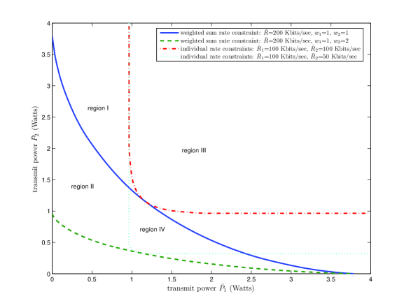
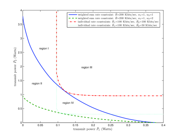
In this section, we present numerical results of our energy-efficient resource allocation for a two-user Rayleigh flat-fading TDMA channel. The available system bandwidth is $B=100$ KHz, and the AWGN has two-sided power spectral density $N_{0}$ Watts/Hz. The user fading processes are independent and the state $h_{k}$, $k=1,2$, is subject to Rayleigh fading with mean $\bar{h}_{k}$. Clearly, the signal-to-noise ratio (SNR) for user $k$ is defined as $\bar{h}_{k}/(N_{0}B)$.

Supposing $\bar{h}_{k}/(N_{0}B)=0$ dBW, $k=1,2$, we test energy-efficient resource allocation under a weighted sum average rate constraint $\bar{R}=200$ Kbits/sec, for two different sets of rate-reward weights: i) $w_{1}=1$, $w_{2}=1$, and ii) $w_{1}=1$, $w_{2}=2$; and the resource allocation under two different sets of individual rate constraints: iii) $\bar{R}_{1}=100$ Kbits/sec, $\bar{R}_{2}=100$ Kbits/sec, and iv) $\bar{R}_{1}=100$ Kbits/sec, $\bar{R}_{2}=50$ Kbits/sec. Fig. 3 depicts the power regions of the Rayleigh fading TDMA fading channels for the infinite-codebook case. It is seen that power regions I and III under the weighted sum rate constraint i) and under individual rate constraints iii) are symmetric with respect to the line $\bar{P}_{2}=\bar{P}_{1}$. Since the individual rate constraints can be seen as a realization of the weighted sum-rate constraint, i.e., $w_{1}\bar{R}_{1}+w_{2}\bar{R}_{2}=\bar{R}$, the power region I contains power region III. It is clear that when $\mu_{1}=\mu_{2}$, due to the symmetry in channel quality and rate-reward weights between the two users, the optimal resource allocation should result in $\bar{R}_{1}=\bar{R}_{2}$ under the weighted sum rate constraint. For this reason, the two power regions touch each other in this case. The relation between power regions II and IV under the weighted sum average rate constraint ii) and under individual rate constraints iv), are similar. They are not symmetric with respect to $\bar{P}_{2}=\bar{P}_{1}$ due to the unbalanced rate-reward weights or individual rate constraints. Power region II contains power region IV, and the two regions touch each other at one point.

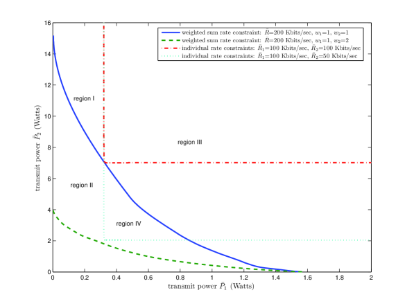
For the finite-AMC-mode case, we assume henceforth that each user supports three $M$-ary quadrature amplitude modulation (QAM) modes: 4-QAM, 16-QAM and 64-QAM. For these rectangular signal constellations, the SEP is given by [19, Chapter 5]

$$P_{M}=1-(1-P_{\sqrt{M}})^{2},$$ (64)

where $P_{\sqrt{M}}=2\left(1-\frac{1}{\sqrt{M}}\right)Q\left(\sqrt{\frac{3}{M-1}\frac{p_{k}h_{k}}{N_{0}B}}\right),$ and $Q(x):=\int_{x}^{\infty}(1/\sqrt{2\pi})e^{-y^{2}/2}dy$ is the Marcum’s Q-function. From (64), we determine the rate-power pair $\{(\rho_{k,l},p_{k,l})\}_{l=1}^{3}$ for user $k=1,2$. The corresponding power regions I-IV under the constraints i)-iv) for this finite-AMC-mode case with prescribed SEP = $10^{-3}$ are shown in Fig. 4. Similar trends as in Fig. 3 are observed. However, the power regions shrink since more power is required to achieve the same transmission rate in the finite-AMC-mode case relative to that in the infinite-codebook case.

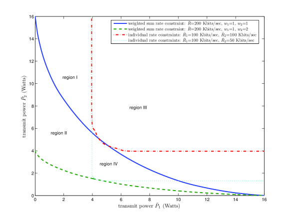
Supposing $\bar{h}_{1}/(N_{0}B)=10$ dBW and $\bar{h}_{1}/(N_{0}B)=0$ dBW, we also test our energy-efficient resource allocation under the same four sets of rate constraints i)-iv). The power regions for the infinite-codebook case and the finite-AMC-mode case are shown in Fig. 5 and Fig. 6, respectively. Since the first user has a significantly better channel (i.e., higher SNR) than user 2, the required transmit power of user 1 is much lower than that of user 2 most of the time. Except this, the results are similar to those in Figs. 3 and 4.

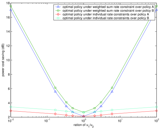
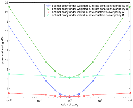
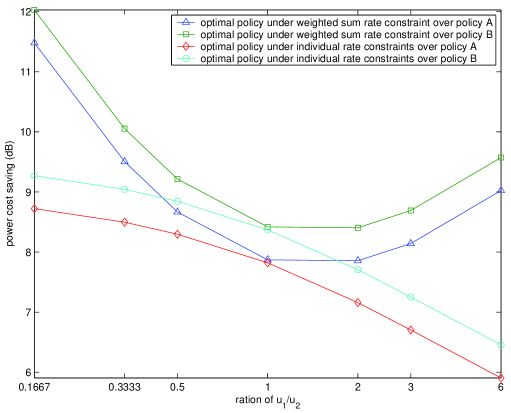
We next compare the derived energy-efficient resource allocation with two alternative resource allocation policies. Policy A assigns equal time fractions to the two users per block. Then each user implements water-filling separately to adapt its transmission rate at each assigned time fraction. In policy B, each user is assigned equal time fraction and transmits with equal power per block. Fig. 7 depicts the power savings of our optimal policies under two different sets of rate constraints i) and iii), over the policies A and B for the infinite-codebook case when two users have identical SNRs. It is seen that when the ratio of two users’ power cost weights is far away 1, our optimal policies under a weighted sum-rate constraint can result in huge power savings (near 20 dB) over the other two sub-optimal polices. However, in this case the optimal policies under individual rate constraints only have a small advantage (around 3 dB) in power savings, over the sub-optimal policies. This is because with the weighted sum average rate constraint, we can employ more flexible policies in time and rate allocations. From Fig. 7, we also observe that the separate water-filling in policy A only achieves small power savings (less than 1 dB) over the equal power strategy in policy B. Fig. 8 depicts the same comparison for the finite-AMC-mode case. The same trends are observed. However, in this case separate water-filling in policy A achieves considerable power savings (4 dB) over the equal power strategy in policy B. Fig. 9 depicts similar power savings for the infinite-codebook case under two different sets of rate constraints ii) and iv), when two users have 10 dB in SNR difference. Similar observations are obtained. But note that the optimal policies under individual rate constraints can also achieve large power savings (near 9 dB), over the sub-optimal policies. In a nutsell, our energy-efficient resource allocation policies may indeed result in large power savings.

VII Concluding Remarks

Given full or quantized CSI at the transmitters, we derived energy-efficient resource allocation strategies for TDMA fading channels. For energy minimization under a weighted average sum-rate constraint, the optimal allocation policies are given by water-filling over realizations of convex envelopes; whereas for energy minimization under average individual rate constraints, the optimal strategies perform greedy water-filling. Comparing these two strategies for two different optimizations, we find that the first approach requires one to characterize the convex envelope of the minima of C$\thicksim$R functions per fading state, but the associated scalar Lagrange multiplier $\lambda^{*}$ can be easily obtained by one-dimensional search. Greedy water-filling simply computes and compares the channel quality indicator functions of individual users and then picks the user(s) with best channel(s) to transmit per block; however, we need to iteratively compute the associated vector Lagrange multiplier $\boldsymbol{\lambda}^{*}$ (by Algorithm 4).

An interesting feature of our energy-efficient resource allocation strategies should be stressed. According to our policies, we can let the access point (which naturally has full CSI) decide the time allocation and feed it back to users via uplink map messages, as in e.g., IEEE 802.16 systems [20]. Then given the Lagrange constant $\lambda^{*}$ (with the weighted sum-rate constraint) or vector $\boldsymbol{\lambda}^{*}$ (with the individual rate constraints), the user only needs its own CSI to determine the transmission rate at the assigned time fraction. If uplink and downlink transmissions are operated in a time-division duplexing (TDD) mode, the users can even obtain their own CSI without feedback from the access point. Together with the fact that the access point needs only a few bits to indicate the time allocation (since most of the time we should allow only one user to transmit), this feature is attractive from a practical implementation viewpoint.

As far as future work, it is interesting to study energy minimization over fading channels with delay constraint and/or using quantized CSI throughout. Our energy minimization for finite-AMC modes only requires quantized CSI feedback from the access point. And delay-constrained energy minimization may be seen as the dual problem of the delay-limited capacity maximization in [10]. Extensions to these two directions are currently under investigation.

Appendices

VII-A Proof of Lemmas 1 and 2

A1. Proof of Lemma 1: The $k$th derivatives of $f_{2}(x)$ and $f_{1}(x)$ are given by

$$f_{2}^{(k)}(x)=\frac{(\ln 2)^{k}\mu_{2}}{w_{2}^{k}h_{2}}2^{\frac{x}{w_{2}}},\qquad f_{1}^{(k)}(x)=\frac{(\ln 2)^{k}\mu_{1}}{w_{1}^{k}h_{1}}2^{\frac{x}{w_{1}}}.$$ (65)

1. If $\frac{\mu_{1}}{w_{1}h_{1}}\geq\frac{\mu_{2}}{w_{2}h_{2}}$, since $2^{\frac{x}{w_{2}}}<2^{\frac{x}{w_{1}}}$ for $w_{1}<w_{2}$, we have $f_{2}^{(1)}(x)<f_{1}^{(1)}(x)$, $\forall x>0$. Since $f_{2}(0)=f_{1}(0)$, we readily infer that $f_{2}(x)<f_{1}(x)$, $\forall x>0$.

2. If $\frac{\mu_{1}}{w_{1}h_{1}}<\frac{\mu_{2}}{w_{2}h_{2}}$, since $w_{1}<w_{2}$, there exists $k>1$ such that $\frac{(\ln 2)^{k}\mu_{2}}{w_{2}^{k}h_{2}}\leq\frac{(\ln 2)^{k}\mu_{1}}{w_{1}^{k}h_{1}}$. Let $k_{0}=\min_{k}\;\arg\left\{\frac{(\ln 2)^{k}\mu_{2}}{w_{2}^{k}h_{2}}\leq\frac{(\ln 2)^{k}\mu_{1}}{w_{1}^{k}h_{1}}\right\}$. Together with $2^{\frac{x}{w_{2}}}<2^{\frac{x}{w_{1}}}$, we have $f_{2}^{(k_{0})}(x)<f_{1}^{(k_{0})}(x)$, $\forall x\geq 0$. Since $f_{2}^{(k_{0}-1)}(0)>f_{1}^{(k_{0}-1)}(0)$ and $f_{2}^{(k_{0})}(x)<f_{1}^{(k_{0})}(x)$, we infer that $f_{2}^{(k_{0}-1)}(x)-f_{1}^{(k_{0}-1)}(x)$ starts positive and with a negative slope it crosses the $x$-axis at some point $v_{k_{0}-1}$; hence,

   $$\begin{cases}f_{2}^{(k_{0}-1)}(x)>f_{1}^{(k_{0}-1)}(x)&\mbox{when }0\leq x<v_{k_{0}-1},\\ f_{2}^{(k_{0}-1)}(x)<f_{1}^{(k_{0}-1)}(x)&\mbox{when }x>v_{k_{0}-1};\end{cases}$$ (66)

   Using (66) and $f_{2}^{(k_{0}-2)}(0)>f_{1}^{(k_{0}-2)}(0)$, we obtain similar results for $f_{2}^{(k_{0}-2)}(x)$ and $f_{1}^{(k_{0}-2)}(x)$ with $v_{k_{0}-2}>v_{k_{0}-1}$. By induction, we therefore deduce that

   $$\begin{cases}f_{2}(x)>f_{1}(x)&\mbox{when }0\leq x<v_{0},\\ f_{2}(x)<f_{1}(x)&\mbox{when }x>v_{0};\end{cases}$$ (67)

   where $v_{0}$ is the unique solution of the equation $f_{2}(x)=f_{1}(x)$.

A2. Proof of Lemma 2: For notational brevity, we drop the dependence of $R$, $R_{k}$, $\tau_{k}$ ($k=1,2$), $R_{a}$, $R_{b}$, and $s_{0}$ on $\mathbf{h}$. And we let $\tau_{1}=\tau$ and $\tau_{2}=1-\tau$.

1. When $w_{1}<w_{2}$ and $\frac{\mu_{1}}{w_{1}h_{1}}\geq\frac{\mu_{2}}{w_{2}h_{2}}$, we have from Lemma 1 $f_{2}(x)<f_{1}(x)$, $\forall x>0$. We wish to solve (8) under the constraint $\tau R_{1}+(1-\tau)R_{2}=R$ with $R_{1}\geq 0$ and $R_{2}\geq 0$. Then the cost function satisfies

   $$\tau f_{1}(R_{1})+(1-\tau)f_{2}(R_{2})\geq\tau f_{2}(R_{1})+(1-\tau)f_{2}(R_{2})\geq f_{2}(R),$$ (68)

   where the last inequality is due to the convexity of $f_{2}(R)$, and the equalities are achieved when $\tau=0$, $R_{1}=0$ and $R_{2}=R$. Inequality (68) clearly shows that the minimum in (8) is achieved; i.e., $J(R)=f_{2}(R)$.

2. When $w_{1}<w_{2}$ and $\frac{\mu_{1}}{w_{1}h_{1}}<\frac{\mu_{2}}{w_{2}h_{2}}$, $f_{1}(R)$ and $f_{2}(R)$ intersect as depicted in Fig. 1. Similar to [11, Proof of Lemma 1], we can specify two points $R_{a}$ and $R_{b}$ such that $f_{1}^{(1)}(R_{a})=f_{2}^{(1)}(R_{b})=s_{0}$; i.e., at these two points first-order derivatives of $f_{1}(R)$ and $f_{2}(R)$ are equal:

   $$f_{1}^{(1)}(R_{a})=\frac{\ln 2\mu_{1}}{w_{1}h_{1}}2^{\frac{R_{a}}{w_{1}}}=s_{0};\quad\quad f_{2}^{(1)}(R_{b})=\frac{\ln 2\mu_{2}}{w_{2}h_{2}}2^{\frac{R_{b}}{w_{2}}}=s_{0}.$$ (69)

   The $R_{a}$, $R_{b}$ expressions are obtained after solving (69) for $R_{a}$ and $R_{b}$. Since $s_{0}$ is the slope of the common tangent line of the curves $f_{1}(R)$ and $f_{2}(R)$, we also have

   $$s_{0}=\frac{f_{2}(R_{b})-f_{1}(R_{a})}{R_{b}-R_{a}}.$$ (70)

   Solving (69) and (70), we obtain $s_{0}$ as the solution to $g(x,\mathbf{h})=0$, where $g(x,\mathbf{h})$ is given by (13), and $R_{a}$ and $R_{b}$ are as in (12). If $0<R<R_{a}$ or $R>R_{b}$, then $J(R)$ simply equals to $f_{1}(R)$ or $f_{2}(R)$. If $R_{a}<R<R_{b}$, then $J(R)$ should take the values between $f_{1}(R_{a})$ and $f_{2}(R_{b})$ on the straight line, and $J(R)$ can be achieved by time-sharing; i.e., $R=\tau R_{a}+(1-\tau)R_{b}$, and $J(R)=\tau f_{1}(R_{a})+(1-\tau)f_{2}(R_{b})$. The optimal resource allocation per fading state is thus given by (14)-(16).

VII-B Proof of Theorem 1

Let $R^{*}(\mathbf{h})$ denote the optimal total rate reward assigned to fading state $\mathbf{h}$, and $r_{k}^{*}(\mathbf{h})$ and $\tau_{k}^{*}(\mathbf{h})$ the corresponding optimal rate and time fraction allocated to user $k=1,2$. To solve (9), we rely on the Karush-Kuhn-Tucker (KKT) conditions [16, Chapter 5]. Let $J^{(1)}(R(\mathbf{h}))$ denote first derivative of $J(R(\mathbf{h}))$ with respect to $R(\mathbf{h})$. Taking the partial derivative of $E_{\mathbf{h}}[J(R(\mathbf{h}))]-\lambda E_{\mathbf{h}}[R(\mathbf{h})]$ in (9) with respect to $R(\mathbf{h})$ for a fixed $\mathbf{h}$, only $J^{(1)}(R(\mathbf{h}))-\lambda$ survives since all $R(\mathbf{h^{\prime}})$ for realizations $\mathbf{h^{\prime}}\neq\mathbf{h}$ are regarded as constants. We thus have at the optimum that if $R^{*}(\mathbf{h})>0$,

$$J^{(1)}(R^{*}(\mathbf{h}))=\lambda^{*}.$$ (71)

1. If $\frac{\mu_{1}}{w_{1}h_{1}}\geq\frac{\mu_{2}}{w_{2}h_{2}}$, then $J(R(\mathbf{h}))=f_{2}(R(\mathbf{h}))$ from Lemma 2, and thus $J^{(1)}(R(\mathbf{h}))=\frac{\ln 2\mu_{2}}{w_{2}h_{2}}2^{\frac{R(\mathbf{h})}{w_{2}}}$. Substituting the latter into (71) and recalling that $R(\mathbf{h})\geq 0$, we find

   $$R^{*}(\mathbf{h})=w_{2}\left[\log\frac{\lambda^{*}w_{2}h_{2}}{\ln 2\mu_{2}}\right]_{+}=w_{2}\left[\log\lambda^{*}-\log\frac{\ln 2\mu_{2}}{w_{2}h_{2}}\right]_{+},$$ (72)

   which yields the optimal rate and time allocation in (17).

2. If $\frac{\mu_{1}}{w_{1}h_{1}}<\frac{\mu_{2}}{w_{2}h_{2}}$ and we recall that $s_{0}$ is the slope of the straight line segment in Fig. 1, it follows from Lemma 2 that

   $$\begin{cases}\mbox{if}\;\;0<R^{*}(\mathbf{h})<R_{a},&\lambda^{*}=J^{(1)}(R^{*}(\mathbf{h}))<s_{0};\\ \mbox{if}\;\;R_{a}\leq R^{*}(\mathbf{h})\leq R_{b},&\lambda^{*}=J^{(1)}(R^{*}(\mathbf{h}))=s_{0};\\ \mbox{if}\;\;R^{*}(\mathbf{h})>R_{b},&\lambda^{*}=J^{(1)}(R^{*}(\mathbf{h}))>s_{0};\end{cases}$$ (73)

   where $R_{a}$, $R_{b}$ and $s_{0}$ are functions of $\mathbf{h}$, given in Lemma 2. Now using (73), we arrive at:

   1. If $\lambda^{*}<s_{0}$, then $J(R(\mathbf{h}))=f_{1}(R(\mathbf{h}))$, and thus $R^{*}(\mathbf{h})=w_{1}\left[\log\lambda^{*}-\log\frac{\ln 2\mu_{1}}{w_{1}h_{1}}\right]_{+}$; which in turn yields the optimal rate and time allocation in (18).

   2. If $\lambda^{*}>s_{0}$, then $J(R(\mathbf{h}))=f_{2}(R(\mathbf{h}))$, and thus $R^{*}(\mathbf{h})=w_{2}\left[\log\lambda^{*}-\log\frac{\ln 2\mu_{2}}{w_{2}h_{2}}\right]_{+}$, which in turn yields the optimal rate and time allocation in (19).

   3. If $\lambda^{*}=s_{0}$, then $J(R(\mathbf{h}))=f_{1}(R_{a})+s_{0}(R(\mathbf{h})-R_{a})$, and $R^{*}(\mathbf{h})$ can be any value between $R_{a}$ and $R_{b}$. In this case, we obtain the optimal rate and time allocation (20).

   Since $R_{a}<R_{b}$, we have from (12)

   $$w_{1}\log\frac{s_{0}w_{1}h_{1}}{\ln 2\mu_{1}}<w_{2}\log\frac{s_{0}w_{2}h_{2}}{\ln 2\mu_{2}}\quad\Rightarrow\quad s_{0}>\left(\frac{((w_{1}h_{1})/(\ln 2\mu_{1}))^{w_{1}}}{((w_{2}h_{2})/(\ln 2\mu_{2}))^{w_{2}}}\right)^{\frac{1}{w_{2}-w_{1}}}:=\xi.$$ (74)

   Moreover, since $g(s_{0},\mathbf{h})=0$, and $g^{(1)}(x,\mathbf{h})=w_{2}\log\frac{xw_{2}h_{2}}{\ln 2\mu_{2}}-w_{1}\log\frac{xw_{1}h_{1}}{\ln 2\mu_{1}}$, it follows from (74) that

   $$\begin{cases}g^{(1)}(x,\mathbf{h})<0,&\mbox{for}\;\;0<x<\xi;\\ g^{(1)}(x,\mathbf{h})>0,&\mbox{for}\;\;x>\xi.\end{cases}$$ (75)

   Therefore, we have:

   1. If $\lambda^{*}<\xi$ or $\lambda^{*}>\xi$ and $g(\lambda^{*},\mathbf{h})<0$, then $\lambda^{*}<s_{0}$.

   2. If $\lambda^{*}>\xi$ and $g(\lambda^{*},\mathbf{h})>0$, then $\lambda^{*}>s_{0}$.

   3. If $\lambda^{*}>\xi$ and $g(\lambda^{*},\mathbf{h})=0$, then $\lambda^{*}=s_{0}$.

   Combining a’), b’), c’) with a), b), c) proves the second part of Theorem 1.

VII-C Proof of Theorem 2

Since $\bar{f}(x):=\min_{1\leq k\leq K}f_{k}(x)$, it is easy to show that

$$J(R(\mathbf{h})):=\min_{\mathbf{r}(\mathbf{h}),\boldsymbol{\tau}(\mathbf{h})}\sum_{k=1}^{K}\tau_{k}(\mathbf{h})f_{k}(R_{k}(\mathbf{h}))\geq\min_{\mathbf{r}(\mathbf{h}),\boldsymbol{\tau}(\mathbf{h})}\sum_{k=1}^{K}\tau_{k}(\mathbf{h})\bar{f}(R_{k}(\mathbf{h})).$$ (76)

By the definition of the convex envelope $\bar{f}^{c}(x)$, we have

$$\sum_{k=1}^{K}\tau_{k}(\mathbf{h})\bar{f}(R_{k}(\mathbf{h}))\geq\sum_{k=1}^{K}\tau_{k}(\mathbf{h})\bar{f}^{c}(R_{k}(\mathbf{h}))\geq\bar{f}^{c}\left(\sum_{k=1}^{K}\tau_{k}(\mathbf{h})R_{k}(\mathbf{h})\right):=\bar{f}^{c}(R(\mathbf{h}));$$ (77)

where the last inequality is due to the convexity of $\bar{f}^{c}(x)$. From (76) and (77), it is clear that $J(R(\mathbf{h}))\geq\bar{f}^{c}(R(\mathbf{h}))$.

On the other hand, according to the definition of $\bar{f}^{c}(x)$, for any given $R(\mathbf{h})$ there exists $R_{a}(\mathbf{h})$ and $R_{b}(\mathbf{h})$ (possibly $R_{a}(\mathbf{h})=R_{b}(\mathbf{h})$) and $\tau^{*}$ such that

$$\tau^{*}R_{a}(\mathbf{h})+(1-\tau^{*})R_{b}(\mathbf{h})=R(\mathbf{h});\quad\quad\tau^{*}\bar{f}(R_{a}(\mathbf{h}))+(1-\tau^{*})\bar{f}(R_{b}(\mathbf{h}))=\bar{f}^{c}(R(\mathbf{h})).$$ (78)

Eq. (78) shows that we can achieve the equality $J(R(\mathbf{h}))=\bar{f}^{c}(R(\mathbf{h}))$ by assigning

$$\begin{cases}\tau_{i}^{*}(\mathbf{h})=\tau^{*},&r_{i}^{*}(\mathbf{h})=R_{a}(\mathbf{h})/w_{i}\\ \tau_{j}^{*}(\mathbf{h})=1-\tau^{*},&r_{j}^{*}(\mathbf{h})=R_{b}(\mathbf{h})/w_{j}\end{cases}$$ (79)

to users $i$ and $j$ which satisfy $f_{i}(R_{a}(\mathbf{h}))=\bar{f}(R_{a}(\mathbf{h}))$ and $f_{j}(R_{b}(\mathbf{h}))=\bar{f}(R_{b}(\mathbf{h}))$. This completes the proof.

VII-D Proof of Theorem 3

Letting $M:=\sum_{k=1}^{K}M_{k}$, the value of $K_{0}$ per fading state may take any integer in [1, $M$]. We define $\mathbf{{\cal H}}_{K_{0}}$ as the set of all fading states $\mathbf{h}$ for which Algorithm 3 yields $K_{0}\in[1,M]$. We further set $s_{K_{0}+1}(\mathbf{h})=\infty$, $\forall\lambda>0$, and define for $m=0,1,\ldots,K_{0}$, the sets

$$\mathbf{{\cal H}}_{m}(K_{0},\lambda) := \left\{\mathbf{h}:\;\mathbf{h}\in\mathbf{{\cal H}}_{K_{0}},\;s_{m}(\mathbf{h})<\lambda<s_{m+1}(\mathbf{h})\right\},$$ (80)

$$\tilde{\mathbf{{\cal H}}}_{m}(K_{0},\lambda) := \left\{\mathbf{h}:\;\mathbf{h}\in\mathbf{{\cal H}}_{K_{0}},\;\lambda=s_{m}(\mathbf{h})\right\}.$$ (81)

Then $\forall\lambda>0$, since $\tilde{\mathbf{{\cal H}}}_{0}(K_{0},\lambda)=\phi$, we can express the set $\mathbf{{\cal H}}$ of all possible fading states as

$$\mathbf{{\cal H}}=\bigcup_{1\leq K_{0}\leq M}\;\mathbf{{\cal H}}_{K_{0}}=\bigcup_{1\leq K_{0}\leq M}\;\left\{\mathbf{{\cal H}}_{0}(K_{0},\lambda)\cup\bigcup_{1\leq m\leq K_{0}}\;\left(\mathbf{{\cal H}}_{m}(K_{0},\lambda)\cup\tilde{\mathbf{{\cal H}}}_{m}(K_{0},\lambda)\right)\right\}.$$ (82)

Using the defined partitions $\mathbf{{\cal H}}_{K_{0}}$, we can rewrite (34) as

$$\begin{cases}\min_{\boldsymbol{\tilde{\tau}}(\mathbf{h})}\;\sum_{K_{0}=1}^{M}\;E_{\mathbf{h}\in\mathbf{{\cal H}}_{K_{0}}}\left[\sum_{m=1}^{K_{0}}\tilde{\tau}_{m}(\mathbf{h})C_{m}(\mathbf{h})\right]\\ \mbox{subject to}\quad\quad\sum_{K_{0}=1}^{M}\;E_{\mathbf{h}\in\mathbf{{\cal H}}_{K_{0}}}\left[\sum_{m=1}^{K_{0}}\tilde{\tau}_{m}(\mathbf{h})R_{m}(\mathbf{h})\right]\geq\bar{R},\quad\sum_{m=1}^{K_{0}}\tilde{\tau}_{m}(\mathbf{h})=1.\end{cases}$$ (83)

If the optimization is feasible, we have

$$\sum_{K_{0}=1}^{M}\;E_{\mathbf{h}\in\mathbf{{\cal H}}_{K_{0}}}\left[R_{K_{0}}(\mathbf{h})\right]\;\geq\bar{R}.$$ (84)

It is easy to show that we can always achieve (37) although the solution for $\tau_{0}^{*}$ may not be unique.

In the following, $\forall K_{0}\in[1,M]$ and $\forall m\in[1,K_{0}]$, we drop the dependence of $\tilde{\tau}_{m}$, $\tilde{\tau}_{m}^{*}$, $R_{m}$, $C_{m}$ and $s_{m}$ on $\mathbf{h}$ for notational brevity. For $K_{0}\in[1,M]$ and $\forall\mathbf{h}\in\mathbf{{\cal H}}_{K_{0}}$, we let

$$\boldsymbol{\tilde{\tau}}^{*}:=[\tilde{\tau}_{1}^{*},\ldots,\tilde{\tau}_{K_{0}}^{*}]^{T},\quad\quad\boldsymbol{\tilde{\tau}}:=[\tilde{\tau}_{1},\ldots,\tilde{\tau}_{K_{0}}]^{T}.$$ (85)

The $\boldsymbol{\tilde{\tau}}^{*}$ given by the theorem satisfies

$$\sum_{K_{0}=1}^{M}\;E_{\mathbf{h}\in\mathbf{{\cal H}}_{K_{0}}}\left[\sum_{m=1}^{K_{0}}\tilde{\tau}_{m}^{*}R_{m}\right]=\bar{R}.$$ (86)

From the definition of $\{\mathbf{{\cal H}}_{m}(K_{0},\lambda^{*})\}_{m=0}^{K_{0}}$ and $\{\tilde{\mathbf{{\cal H}}}_{m}(K_{0},\lambda^{*})\}_{m=1}^{K_{0}}$, we have $\forall\boldsymbol{\tilde{\tau}}\neq\boldsymbol{\tilde{\tau}}^{*}$ that

$$\sum_{K_{0}=1}^{M}\;E_{\mathbf{h}\in\mathbf{{\cal H}}_{K_{0}}}\left[\sum_{m=1}^{K_{0}}\tilde{\tau}_{m}R_{m}\right]-\bar{R}$$ (87)

$$= \sum_{K_{0}=1}^{M}\;E_{\mathbf{h}\in\mathbf{{\cal H}}_{K_{0}}}\left[\sum_{m=1}^{K_{0}}\tilde{\tau}_{m}R_{m}\right]-\sum_{K_{0}=1}^{M}\;E_{\mathbf{h}\in\mathbf{{\cal H}}_{K_{0}}}\left[\sum_{m=1}^{K_{0}}\tilde{\tau}_{m}^{*}R_{m}\right]$$

$$= \sum_{K_{0}=1}^{M}\;\int_{\mathbf{h}\in\mathbf{{\cal H}}_{0}(K_{0},\lambda^{*})}\sum_{i=1}^{K_{0}}\tilde{\tau}_{i}R_{i}\;dF(\mathbf{h})$$

$$+\sum_{K_{0}=1}^{M}\;\sum_{m=1}^{K_{0}}\int_{\mathbf{h}\in\mathbf{{\cal H}}_{m}(K_{0},\lambda^{*})}\left(\sum_{i=1}^{K_{0}}\tilde{\tau}_{i}R_{i}-R_{m}\right)\;dF(\mathbf{h})$$

$$+\sum_{K_{0}=1}^{M}\;\sum_{m=1}^{K_{0}}\int_{\mathbf{h}\in\tilde{\mathbf{{\cal H}}}_{m}(K_{0},\lambda^{*})}\left(\sum_{i=1}^{K_{0}}\tilde{\tau}_{i}R_{i}-\tau_{0}^{*}R_{m}-(1-\tau_{0}^{*})R_{m-1}\right)\;dF(\mathbf{h}).$$

By the convexity of $J(R(\mathbf{h}))$, we can easily show that

$$\frac{C_{m-1}}{R_{m-1}}<\frac{C_{m}}{R_{m}},\quad\quad m=2,\ldots,K_{0}.$$ (88)

1. $\forall\mathbf{h}\in\mathbf{{\cal H}}_{0}(K_{0},\lambda^{*})$, since $\lambda^{*}<s_{1}=C_{1}/R_{1}$, we have from (88) that $\lambda^{*}<C_{i}/R_{i}$, $\forall i\in[1,K_{0}]$, i.e., $R_{i}<C_{i}/\lambda^{*}$. Then the first summand of the last equality in (87) will be

   $$\sum_{K_{0}=1}^{M}\;\int_{\mathbf{h}\in\mathbf{{\cal H}}_{0}(K_{0},\lambda^{*})}\sum_{i=1}^{K_{0}}\tilde{\tau}_{i}R_{i}\;dF(\mathbf{h})\leq\frac{1}{\lambda^{*}}\sum_{K_{0}=1}^{M}\;\int_{\mathbf{h}\in\mathbf{{\cal H}}_{0}(K_{0},\lambda^{*})}\sum_{i=1}^{K_{0}}\tilde{\tau}_{i}C_{i}\;dF(\mathbf{h}).$$ (89)

2. $\forall\mathbf{h}\in\mathbf{{\cal H}}_{m}(K_{0},\lambda^{*})$, $m=1,\ldots,K_{0}$, since $s_{m}<\lambda^{*}<s_{m+1}$, we have

   $$R_{m+1}<R_{m}+(C_{m+1}-C_{m})/\lambda^{*},\quad\quad R_{m-1}<R_{m}+(C_{m-1}-C_{m})/\lambda^{*}.$$ (90)

   Using convexity, we have $s_{i}<\lambda^{*}<s_{k}$, $\forall i\in[1,m-1]$, $\forall k\in[m+1,K_{0}]$. Hence $\forall i\neq m$, $i\in[1,K_{0}]$, we have $R_{i}<R_{m}+(C_{i}-C_{m})/\lambda^{*}$. Then the second summand in (87) will be

   $$\sum_{K_{0}=1}^{M}\;\sum_{m=1}^{K_{0}}\int_{\mathbf{h}\in\mathbf{{\cal H}}_{m}(K_{0},\lambda^{*})}\left(\sum_{i=1}^{K_{0}}\tilde{\tau}_{i}R_{i}-R_{m}\right)\;dF(\mathbf{h})$$ (91)

   $$\leq \sum_{K_{0}=1}^{M}\;\sum_{m=1}^{K_{0}}\int_{\mathbf{h}\in\mathbf{{\cal H}}_{m}(K_{0},\lambda^{*})}\left(\sum_{i\neq m,\;i=1}^{K_{0}}\tilde{\tau}_{i}[R_{m}+(C_{i}-C_{m})/\lambda^{*}]\;+\tilde{\tau}_{m}R_{m}-R_{m}\right)\;dF(\mathbf{h})$$

   $$= \sum_{K_{0}=1}^{M}\;\sum_{m=1}^{K_{0}}\int_{\mathbf{h}\in\mathbf{{\cal H}}_{m}(K_{0},\lambda^{*})}\left(\sum_{i\neq m,\;i=1}^{K_{0}}\tilde{\tau}_{i}(C_{i}-C_{m})/\lambda^{*}\right)\;dF(\mathbf{h})$$

   $$= \frac{1}{\lambda^{*}}\sum_{K_{0}=1}^{M}\;\sum_{m=1}^{K_{0}}\int_{\mathbf{h}\in\mathbf{{\cal H}}_{m}(K_{0},\lambda^{*})}\left(\sum_{i=1}^{K_{0}}\tilde{\tau}_{i}C_{i}-C_{m}\right)\;dF(\mathbf{h}).$$

3. $\forall\mathbf{h}\in\tilde{\mathbf{{\cal H}}}_{m}(K_{0},\lambda^{*})$, $m\in[1,K_{0}]$ and since $\lambda^{*}=s_{m}$, we have $R_{m-1}=R_{m}+(C_{m-1}-C_{m})/\lambda^{*}$. Since $\forall i\in[1,m-1]$, $\forall k\in[m+1,K_{0}]$, we have $s_{i}<\lambda^{*}<s_{k}$, from which it follows that $R_{i}<R_{m}+(C_{i}-C_{m})/\lambda^{*}$, $\forall i\neq m,m-1$ and $i\in[1,K_{0}]$. Then the third summand in (87) will be

   $$\sum_{K_{0}=1}^{M}\;\sum_{m=1}^{K_{0}}\int_{\mathbf{h}\in\tilde{\mathbf{{\cal H}}}_{m}(K_{0},\lambda^{*})}\left(\sum_{i=1}^{K_{0}}\tilde{\tau}_{i}R_{i}-\tau_{0}^{*}R_{m}-(1-\tau_{0}^{*})R_{m-1}\right)\;dF(\mathbf{h})$$ (92)

   $$\leq \sum_{K_{0}=1}^{M}\;\sum_{m=1}^{K_{0}}\int_{\mathbf{h}\in\tilde{\mathbf{{\cal H}}}_{m}(K_{0},\lambda^{*})}\left(\sum_{i\neq m,\;i=1}^{K_{0}}\tilde{\tau}_{i}[R_{m}+(C_{i}-C_{m})/\lambda^{*}]\right.$$

   $$\hskip 128.0374pt\Biggl{.}+\tilde{\tau}_{m}R_{m}-\tau_{0}^{*}R_{m}-(1-\tau_{0}^{*})R_{m-1}\Biggr{)}\;dF(\mathbf{h})$$

   $$= \sum_{K_{0}=1}^{M}\;\sum_{m=1}^{K_{0}}\int_{\mathbf{h}\in\tilde{\mathbf{{\cal H}}}_{m}(K_{0},\lambda^{*})}\left(\sum_{i\neq m,\;i=1}^{K_{0}}\tilde{\tau}_{i}(C_{i}-C_{m})/\lambda^{*}\;+(1-\tau_{0}^{*})(R_{m}-R_{m-1})\right)\;dF(\mathbf{h})$$

   $$= \frac{1}{\lambda^{*}}\sum_{K_{0}=1}^{M}\;\sum_{m=1}^{K_{0}}\int_{\mathbf{h}\in\tilde{\mathbf{{\cal H}}}_{m}(K_{0},\lambda^{*})}\left(\sum_{i=1}^{K_{0}}\tilde{\tau}_{i}C_{i}-\tau_{0}^{*}C_{m}-(1-\tau_{0}^{*})C_{m-1}\right)\;dF(\mathbf{h}).$$

Substituting (89), (91) and (92) into (87), we find

$$\sum_{K_{0}=1}^{M}\;E_{\mathbf{h}\in\mathbf{{\cal H}}_{K_{0}}}\left[\sum_{m=1}^{K_{0}}\tilde{\tau}_{m}R_{m}\right]-\bar{R}$$ (93)

$$\leq \frac{1}{\lambda^{*}}\sum_{K_{0}=1}^{M}\left\{\int_{\mathbf{h}\in\mathbf{{\cal H}}_{0}(K_{0},\lambda^{*})}\sum_{i=1}^{K_{0}}\tilde{\tau}_{i}C_{i}\;dF(\mathbf{h})\right.$$

$$\hskip 56.9055pt+\sum_{m=1}^{K_{0}}\int_{\mathbf{h}\in\mathbf{{\cal H}}_{m}(K_{0},\lambda^{*})}\left(\sum_{i=1}^{K_{0}}\tilde{\tau}_{i}C_{i}-C_{m}\right)\;dF(\mathbf{h})$$

$$\hskip 56.9055pt\left.+\sum_{m=1}^{K_{0}}\int_{\mathbf{h}\in\tilde{\mathbf{{\cal H}}}_{m}(K_{0},\lambda^{*})}\left(\sum_{i=1}^{K_{0}}\tilde{\tau}_{i}C_{i}-\tau_{0}^{*}C_{m}-(1-\tau_{0}^{*})C_{m-1}\right)\;dF(\mathbf{h})\right\}$$

$$= \frac{1}{\lambda^{*}}\left\{\sum_{K_{0}=1}^{M}\;E_{\mathbf{h}\in\mathbf{{\cal H}}_{K_{0}}}\left[\sum_{m=1}^{K_{0}}\tilde{\tau}_{m}C_{m}\right]-\sum_{K_{0}=1}^{M}\;E_{\mathbf{h}\in\mathbf{{\cal H}}_{K_{0}}}\left[\sum_{m=1}^{K_{0}}\tilde{\tau}_{m}^{*}C_{m}\right]\right\}.$$

Therefore, $\forall\boldsymbol{\tilde{\tau}}\neq\boldsymbol{\tilde{\tau}}^{*}$, if $\boldsymbol{\tilde{\tau}}$ satisfies the total average-rate constraint $\sum_{K_{0}=1}^{M}\;E_{\mathbf{h}\in\mathbf{{\cal H}}_{K_{0}}}\left[\sum_{m=1}^{K_{0}}\tilde{\tau}_{m}R_{m}\right]\geq\bar{R}$, we have

$$\sum_{K_{0}=1}^{M}\;E_{\mathbf{h}\in\mathbf{{\cal H}}_{K_{0}}}\left[\sum_{m=1}^{K_{0}}\tilde{\tau}_{m}C_{m}\right]\geq\sum_{K_{0}=1}^{M}\;E_{\mathbf{h}\in\mathbf{{\cal H}}_{K_{0}}}\left[\sum_{m=1}^{K_{0}}\tilde{\tau}_{m}^{*}C_{m}\right].$$ (94)

Hence, $\boldsymbol{\tilde{\tau}}^{*}$ is the optimal solution to (34) and consequently the corresponding $\mathbf{r}^{*}$ and $\boldsymbol{\tau}^{*}$ are the optimal solutions to (31).

VII-E Proof of Theorem 4

Following the Lagrange multiplier method, (40) is equivalent to

$$\begin{cases}\min_{\mathbf{r}(\cdot),\boldsymbol{\tau}(\cdot)}E_{\mathbf{h}}\left[\sum_{k=1}^{K}\mu_{k}\frac{\tau_{k}(\mathbf{h})}{h_{k}}(2^{r_{k}(\mathbf{h})}-1)\right]-\sum_{k=1}^{K}\lambda_{k}E_{\mathbf{h}}[\tau_{k}(\mathbf{h})r_{k}(\mathbf{h})]\\ \mbox{subject to}\quad E_{\mathbf{h}}\left[\tau_{k}(\mathbf{h})r_{k}(\mathbf{h})\right]=\bar{R}_{k},\;\;k=1,\ldots,K,\\ \hskip 56.9055pt\sum_{k=1}^{K}\tau_{k}(\mathbf{h})=1,\;\;\forall\mathbf{h}.\end{cases}$$ (95)

Using the definition of $f_{k}(r_{k}(\mathbf{h}))$, we can rewrite (95) as

$$\begin{cases}\min_{\mathbf{r}(\cdot),\boldsymbol{\tau}(\cdot)}E_{\mathbf{h}}\left[\sum_{k=1}^{K}\tau_{k}(\mathbf{h})f_{k}(r_{k}(\mathbf{h}))\right]\\ \mbox{subject to}\quad E_{\mathbf{h}}\left[\tau_{k}(\mathbf{h})r_{k}(\mathbf{h})\right]=\bar{R}_{k},\;\;k=1,\ldots,K,\\ \hskip 56.9055pt\sum_{k=1}^{K}\tau_{k}(\mathbf{h})=1,\;\;\forall\mathbf{h}.\end{cases}$$ (96)

Due to the feasibility and convexity of the power region $\tilde{{\cal P}}(\mathbf{\bar{r}})$, the original problem (39) has a solution. Therefore, given any $\boldsymbol{\mu}:=[\mu_{1},\ldots,\mu_{K}]^{T}>\mathbf{0}$, there exists a $\boldsymbol{\lambda}^{*}:=[\lambda_{1}^{*},\ldots,\lambda_{K}^{*}]^{T}>\mathbf{0}$, as well as optimal rate and time allocation policies $\mathbf{r}(\cdot)$ and $\boldsymbol{\tau}(\cdot)$ for (95). It is clear that we can again decompose (95) into two sub-problems. Given $\boldsymbol{\lambda}^{*}$, we first calculate $r_{k}^{*}(\mathbf{h})$ and $\tau_{k}^{*}(\mathbf{h})$ by solving (41) and then we determine the water-filling level $\boldsymbol{\lambda}^{*}$ by satisfying individual rate constraints.

Since $f_{k}(r_{k}(\mathbf{h}))$ is convex in $r_{k}(\mathbf{h})$, it is easy to show that it attains its minimum at $r_{k,\min}(\mathbf{h})=\left[\log\lambda_{k}^{*}-\log\frac{\ln 2\mu_{k}}{h_{k}}\right]_{+}$. From the KKT conditions [16, Chapter 5], it follows that for $\tau_{k}^{*}(\mathbf{h})>0$, we should have $r_{k}^{*}(\mathbf{h})=r_{k,\min}(\mathbf{h})$. Next, we show that a time allocation strategy $\boldsymbol{\tau}(\cdot)\neq\boldsymbol{\tau}^{*}(\cdot)$, excluding the arbitrary time sharing when functions $f_{k}(r_{k,\min}(\mathbf{h}))$ have multiple minima, is strictly suboptimal.

Let us first consider the two-user case.

1. Suppose that for a fading state $\mathbf{h}$, we have $f_{1}(r_{1,\min}(\mathbf{h}))<f_{2}(r_{2,\min}(\mathbf{h}))$ and $\boldsymbol{\tau}(\mathbf{h})$ is a time allocation policy different from $\boldsymbol{\tau}^{*}(\mathbf{h})$; i.e., $\tau_{1}(\mathbf{h})=1-\alpha$ and $\tau_{2}(\mathbf{h})=\alpha$ with $\alpha>0$. Consider the power cost $J(\mathbf{h}):=(1-\alpha)f_{1}(r_{1,\min}(\mathbf{h}))+\alpha f_{2}(r_{2,\min}(\mathbf{h}))$, where $r_{2,\min}(\mathbf{h})\geq 0$ by definition.

   1. If $r_{2,\min}(\mathbf{h})=0$, then we can let $\tau_{1}^{\prime}(\mathbf{h})=1$, $r_{1}^{\prime}(\mathbf{h})=r_{1,\min}(\mathbf{h})$, and $\tau_{2}^{\prime}(\mathbf{h})=r_{2}^{\prime}(\mathbf{h})=0$ such that $J^{\prime}(\mathbf{h})=f_{1}(r_{1,\min}(\mathbf{h}))<J(\mathbf{h})$. It is clear that $\tau_{1}^{\prime}(\mathbf{h})r_{1}^{\prime}(\mathbf{h})>\tau_{1}(\mathbf{h})r_{1,\min}(\mathbf{h})$, and since $r_{2,\min}(\mathbf{h})=0$, $\tau_{2}^{\prime}(\mathbf{h})r_{2}^{\prime}(\mathbf{h})=\tau_{2}(\mathbf{h})r_{2,\min}(\mathbf{h})=0$. Therefore, if instead of $\boldsymbol{\tau}(\mathbf{h})$ we adopt $\boldsymbol{\tau}^{\prime}(\mathbf{h})$, we incur lower power cost without violating the average individual rate constraints.

   2. If $r_{2,\min}(\mathbf{h})>0$, we should have $f_{2}^{(1)}(r_{2,\min}(\mathbf{h}))=0$. Let us consider the power cost $J^{\prime}(x,\mathbf{h}):=(1-\alpha+x)f_{1}(r_{1,\min}(\mathbf{h}))+(\alpha-x)f_{2}\left(\frac{\alpha}{\alpha-x}r_{2,\min}(\mathbf{h})\right)$, and define $g(x):=J(\mathbf{h})-J^{\prime}(x,\mathbf{h})$. Since $g(0)=0$ and $g^{(1)}(0)=f_{2}(r_{2,\min}(\mathbf{h}))-f_{1}(r_{1,\min}(\mathbf{h}))>0$, there exists $\Delta\alpha\in(0,\alpha)$ such that $g(\Delta\alpha)>0$. Therefore, we have $\tau_{1}^{\prime}(\mathbf{h})=1-\alpha+\Delta\alpha$, $r_{1}^{\prime}(\mathbf{h})=r_{1,\min}(\mathbf{h})$, $\tau_{2}^{\prime}(\mathbf{h})=\alpha-\Delta\alpha$ and $r_{2}^{\prime}(\mathbf{h})=\frac{\alpha}{\alpha-\Delta\alpha}r_{2,\min}(\mathbf{h})$, such that $J^{\prime}(\Delta\alpha,\mathbf{h})<J(\mathbf{h})$. Since $\tau_{1}^{\prime}(\mathbf{h})r_{1}^{\prime}(\mathbf{h})>\tau_{1}(\mathbf{h})r_{1,\min}(\mathbf{h})$ and $\tau_{2}^{\prime}(\mathbf{h})r_{2}^{\prime}(\mathbf{h})=\tau_{2}(\mathbf{h})r_{2,\min}(\mathbf{h})$, with $\boldsymbol{\tau}^{\prime}(\mathbf{h})$ and $\mathbf{r}^{\prime}(\mathbf{h})$ we can afford a smaller power without violating the average individual rate constraints.

2. For a fading state $\mathbf{h}$ satisfying $f_{1}(r_{1,\min}(\mathbf{h}))>f_{2}(r_{2,\min}(\mathbf{h}))$ and $\tau(\mathbf{h})\neq\tau^{*}(\mathbf{h})$, it can be similarly shown that we can have $J^{\prime}(\mathbf{h})<J(\mathbf{h})$ with alternative resource allocation policies.

Previous considerations show that the optimal resource allocation policies should follow Theorem 4 for the two-user case. Similar arguments extend readily to the general $K$-user case as well.

VII-F Proof of Theorem 5

1. From the optimal rate the time allocation policies, we can directly verify the following fact. For all $k$, if the $k$th component of $\boldsymbol{\lambda}$ increases while other components remain fixed, $\bar{R}_{k}(\boldsymbol{\lambda})$ increases whereas $\bar{R}_{i}(\boldsymbol{\lambda})$ decreases for $i\neq k$. More generally, for any subset ${\cal K}$, if we increase $\lambda_{k}$ for all $k\in{\cal K}$ and hold the remaining $\lambda_{i}$ fixed, $\bar{R}_{i}(\boldsymbol{\lambda})$ decreases for $i\in{\cal K}^{C}$, where superscript $C$ here denotes set-complement.

2. It can be easily verified that when $\boldsymbol{\lambda}=\mathbf{0}$, $\mathbf{\bar{r}}(\boldsymbol{\lambda})=\mathbf{0}$, and as $\boldsymbol{\lambda}\uparrow\boldsymbol{\infty}$, $\mathbf{\bar{r}}(\boldsymbol{\lambda})\uparrow\boldsymbol{\infty}$. This in turn implies that

   1. $\forall\boldsymbol{\lambda}(0)>\mathbf{0}$, there exists $\boldsymbol{\alpha}\leq\boldsymbol{\lambda}(0)$ for which $\mathbf{\bar{r}}(\boldsymbol{\alpha})\leq\mathbf{\bar{r}}$;

   2. $\forall\boldsymbol{\lambda}(0)>\mathbf{0}$, there exists $\boldsymbol{\beta}\geq\boldsymbol{\lambda}(0)$ for which $\mathbf{\bar{r}}(\boldsymbol{\beta})\geq\mathbf{\bar{r}}$.

3. Upon defining the mapping $\Lambda:\;\boldsymbol{\lambda}(l)\rightarrowtail\boldsymbol{\lambda}(l+1)$, we can readily verify from Lemma 3 and i) that:

   1. The vector $\boldsymbol{\lambda}^{*}$ is the unique fixed point of the mapping $T$.

   2. The mapping $\Lambda$ is order preserving; i.e., $\boldsymbol{\lambda}\leq\boldsymbol{\lambda}^{\prime}$ $\Rightarrow$ $\Lambda(\boldsymbol{\lambda})\leq\Lambda(\boldsymbol{\lambda}^{\prime})$.

4. We now establish one more fact.

   1. If $\boldsymbol{\lambda}(0)\geq\Lambda(\boldsymbol{\lambda}(0))$ and we define $\boldsymbol{\lambda}(l):=\Lambda^{l}(\boldsymbol{\lambda}(0))$, $l=0,1,\ldots$, then $\boldsymbol{\lambda}(l)$ is a decreasing sequence and $\boldsymbol{\lambda}(l)\downarrow\boldsymbol{\lambda}^{*}$.

   2. If $\boldsymbol{\lambda}(0)\leq\Lambda(\boldsymbol{\lambda}(0))$, then $\boldsymbol{\lambda}(l)$ is an increasing sequence and $\boldsymbol{\lambda}(l)\uparrow\boldsymbol{\lambda}^{*}$.

   Proof: We verify a) and b) as follows.

   1. By preserving the order, we know that $\boldsymbol{\lambda}(l)$ is decreasing. From ii), there exists a $\boldsymbol{\alpha}\leq\boldsymbol{\lambda}(0)$ for which $\mathbf{\bar{r}}(\boldsymbol{\alpha})\leq\mathbf{\bar{r}}$. In addition, by preserving the order, $\forall l$, we have $\boldsymbol{\lambda}(l)\geq\Lambda^{l}(\boldsymbol{\alpha})$. But since $\mathbf{\bar{r}}(\boldsymbol{\alpha})\leq\mathbf{\bar{r}}$, from i), we know that $\Lambda^{l}(\boldsymbol{\alpha})$ is an increasing sequence. Hence, $\{\boldsymbol{\lambda}(l)\}_{l=1}^{\infty}$ is decreasing and bounded; thus, it must converge to the unique fixed point $\boldsymbol{\lambda}^{*}$.

   2. For $\boldsymbol{\lambda}(0)\leq\Lambda(\boldsymbol{\lambda}(0))$, we can similarly prove the claim.

Relying on i)-iv), we are ready to prove the theorem. Notice that ii) guarantees the existence of points $\boldsymbol{\alpha}(0)$ and $\boldsymbol{\beta}(0)$ such that

$$\mbox{I) }\boldsymbol{\alpha}(0)\leq\boldsymbol{\lambda}(0)\leq\boldsymbol{\beta}(0);\qquad\mbox{II) }\mathbf{\bar{r}}(\boldsymbol{\alpha}(0))\leq\mathbf{\bar{r}};\qquad\mbox{III) }\mathbf{\bar{r}}(\boldsymbol{\beta}(0))\geq\mathbf{\bar{r}}.$$ (97)

Defining $\boldsymbol{\alpha}(l):=\Lambda^{l}(\boldsymbol{\alpha}(0))$ and $\boldsymbol{\beta}(l):=\Lambda^{l}(\boldsymbol{\beta}(0))$, we know from iv) that $\boldsymbol{\alpha}(l)\uparrow\boldsymbol{\lambda}^{*}$ and $\boldsymbol{\beta}(l)\downarrow\boldsymbol{\lambda}^{*}$. By preserving the order $\boldsymbol{\alpha}(l)\leq\boldsymbol{\lambda}(l)\leq\boldsymbol{\beta}(l)$, we have $\boldsymbol{\lambda}(l)\rightarrow\boldsymbol{\lambda}^{*}$.

VII-G Proof of Theorem 6

For all CSI realizations $\mathbf{h}$, let

$$\boldsymbol{\tilde{\tau}}^{*} := [\tilde{\tau}_{1,0}^{*},\ldots,\tilde{\tau}_{1,M_{1}}^{*},\ldots,\tilde{\tau}_{K,0}^{*},\ldots,\tilde{\tau}_{K,M_{K}}^{*}]^{T},$$ (98)

$$\boldsymbol{\tilde{\tau}} := [\tilde{\tau}_{1,0},\ldots,\tilde{\tau}_{1,M_{1}},\ldots,\tilde{\tau}_{K,0},\ldots,\tilde{\tau}_{K,M_{K}}]^{T},$$ (99)

and define $\tilde{\tau}_{k}:=\sum_{l=1}^{M_{k}}\;\tilde{\tau}_{k,l}$. If $\mathbf{\bar{r}}$ is feasible, we have $\boldsymbol{\lambda}^{*}$ for which (59) is satisfied. Let us also define $\mathbf{{\cal H}}_{J}:=\{\mathbf{h}:\;\mbox{$\left\{\varphi_{k}(\mathbf{h})\right\}_{k=1}^{K}$ have $J$ minima}\}$, for $J\in[1,K]$, and users $\{i_{j}\}_{j=1}^{J}$ having the “best” channels. Then $\forall\boldsymbol{\tilde{\tau}}\neq\boldsymbol{\tilde{\tau}}^{*}$, we have

$$\sum_{k=1}^{K}\;\lambda_{k}^{*}\left(E_{\mathbf{h}}\left[\sum_{l=1}^{M_{k}}\tilde{\tau}_{k,l}\rho_{k,l}\right]-\bar{R}_{k}\right)$$ (100)

$$= \sum_{k=1}^{K}\;\lambda_{k}^{*}\left(E_{\mathbf{h}}\left[\sum_{l=1}^{M_{k}}\tilde{\tau}_{k,l}\rho_{k,l}\right]-E_{\mathbf{h}}\left[\sum_{l=1}^{M_{k}}\tilde{\tau}_{k,l}^{*}\rho_{k,l}\right]\right)$$

$$= E_{\mathbf{h}\in\mathbf{{\cal H}}_{1}}\left[\sum_{k\neq i,\;k=1}^{K}\;\left(\lambda_{k}^{*}\sum_{l=1}^{M_{k}}\tilde{\tau}_{k,l}\rho_{k,l}\right)+\lambda_{i}^{*}\left(\sum_{l=1}^{M_{i}}\tilde{\tau}_{i,l}\rho_{i,l}\;-\rho_{i,l_{i}^{*}}\right)\right]$$

$$+\sum_{J=2}^{K}\;E_{\mathbf{h}\in\mathbf{{\cal H}}_{J}}\left[\sum_{k\neq i_{j},\;k=1}^{K}\;\left(\lambda_{k}^{*}\sum_{l=1}^{M_{k}}\tilde{\tau}_{k,l}\rho_{k,l}\right)+\sum_{j=1}^{J}\;\lambda_{i_{j}}^{*}\left(\sum_{l=1}^{M_{i_{j}}}\tilde{\tau}_{i_{j},l}\rho_{i_{j},l}\;-\tau_{j}^{*}\rho_{i_{j},l_{i_{j}}^{*}}\right)\right].$$

1. $\forall\mathbf{h}\in\mathbf{{\cal H}}_{1}$, suppose that user $i$ is selected by $\boldsymbol{\tilde{\tau}}^{*}$ as the user with the best channel. Since $\mu_{k}\gamma_{k,l_{k}^{*}}/h_{k}\leq\lambda_{k}^{*}<\mu_{k}\gamma_{k,l_{k}^{*}+1}/h_{k}$, $k\in[1,K]$, we have $\frac{C_{k,l_{k}^{*}}-C_{k,l_{k}^{*}-1}}{\rho_{k,l_{k}^{*}}-\rho_{k,l_{k}^{*}-1}}\leq\lambda_{k}^{*}<\frac{C_{k,l_{k}^{*}+1}-C_{k,l_{k}^{*}}}{\rho_{k,l_{k}^{*}+1}-\rho_{k,l_{k}^{*}}}$. Therefore,

   $$\rho_{k,l_{k}^{*}-1}\leq\rho_{k,l_{k}^{*}}+(C_{k,l_{k}^{*}-1}-C_{k,l_{k}^{*}})/\lambda_{k}^{*},\quad\quad\rho_{k,l_{k}^{*}+1}<\rho_{k,l_{j}^{*}}+(C_{k,l_{k}^{*}+1}-C_{k,l_{k}^{*}})/\lambda_{k}^{*}.$$ (101)

   By the convexity of $\Upsilon_{k}(x)$, we have $\mu_{k}\gamma_{k,l}/h_{k}<\lambda_{k}^{*}<\mu_{k}\gamma_{k,l^{\prime}}/h_{k}$, $\forall l\in[1,l_{k}^{*}-1]$, $\forall l^{\prime}\in[l_{k}^{*}+1,M_{k}]$. Hence, $\forall l\neq l_{k}^{*}$, $l\in[1,M_{k}]$, we have $\rho_{k,l}<\rho_{k,l_{k}^{*}}+(C_{k,l}-C_{k,l_{k}^{*}})/\lambda_{k}^{*}$. Then the first sum of the last equality in (100) will be

   $$E_{\mathbf{h}\in\mathbf{{\cal H}}_{1}}\left[\sum_{k\neq i,\;k=1}^{K}\;\left(\lambda_{k}^{*}\sum_{l=1}^{M_{k}}\tilde{\tau}_{k,l}\rho_{k,l}\right)+\lambda_{i}^{*}\left(\sum_{l=1}^{M_{i}}\tilde{\tau}_{i,l}\rho_{i,l}\;-\rho_{i,l_{i}^{*}}\right)\right]$$ (102)

   $$\leq E_{\mathbf{h}\in\mathbf{{\cal H}}_{1}}\left[\sum_{k\neq i,\;k=1}^{K}\;\left(\sum_{l\neq l_{k}^{*},\;l=1}^{M_{k}}\tilde{\tau}_{k,l}(C_{k,l}-C_{k,l_{k}^{*}})\;+\lambda_{k}^{*}\tilde{\tau}_{k}\rho_{k,l_{k}^{*}}\right)\right.$$

   $$\hskip 42.67912pt\left.+\sum_{l\neq l_{i}^{*},\;l=1}^{M_{i}}\tilde{\tau}_{i,l}(C_{i,l}-C_{i,l_{i}^{*}})+\lambda_{i}^{*}\tilde{\tau}_{i}\rho_{i,l_{i}^{*}}-\lambda_{i}^{*}\rho_{i,l_{i}^{*}}\right]$$

   $$= E_{\mathbf{h}\in\mathbf{{\cal H}}_{1}}\left[\sum_{k\neq i,\;k=1}^{K}\;\left(\sum_{l=1}^{M_{k}}\tilde{\tau}_{k,l}C_{k,l}\;-\tilde{\tau}_{k}(C_{k,l_{k}^{*}}-\lambda_{k}^{*}\rho_{k,l_{k}^{*}})\right)\right.$$

   $$\hskip 42.67912pt\left.+\sum_{l=1}^{M_{i}}\tilde{\tau}_{i,l}C_{i,l}\;-\tilde{\tau}_{i}(C_{i,l_{i}^{*}}-\lambda_{i}^{*}\rho_{i,l_{i}^{*}})-\lambda_{i}^{*}\rho_{i,l_{i}^{*}}\right]$$

   $$\leq E_{\mathbf{h}\in\mathbf{{\cal H}}_{1}}\left[\sum_{k=1}^{K}\;\sum_{l=1}^{M_{k}}\tilde{\tau}_{k,l}C_{k,l}\;-\sum_{k=1}^{K}\tilde{\tau}_{k}(C_{i,l_{i}^{*}}-\lambda_{i}^{*}\rho_{i,l_{i}^{*}})-\lambda_{i}^{*}\rho_{i,l_{i}^{*}}\right]$$

   $$= E_{\mathbf{h}\in\mathbf{{\cal H}}_{1}}\left[\sum_{k=1}^{K}\;\sum_{l=1}^{M_{k}}\tilde{\tau}_{k,l}C_{k,l}\;-C_{i,l_{i}^{*}}\right];$$ (103)

   where we used the allocation policies $\forall k\neq i$, $C_{k,l_{k}^{*}}-\lambda_{k}^{*}\rho_{k,l_{k}^{*}}>C_{i,l_{i}^{*}}-\lambda_{i}^{*}\rho_{i,l_{i}^{*}}$ to obtain inequality (102).

2. $\forall\mathbf{h}\in\mathbf{{\cal H}}_{J}$, $J>1$, suppose that users $i_{j}$ are selected by $\boldsymbol{\tilde{\tau}}^{*}$ as the users with best channels, and define $C_{\min}:=C_{i_{j},l_{i_{j}}^{*}}-\lambda_{i_{j}}^{*}\rho_{i_{j},l_{i_{j}}^{*}}$, $j=1,\ldots,J$. Noticing that $\forall k\neq i_{j}$, $C_{k,l_{k}^{*}}-\lambda_{k}^{*}\rho_{k,l_{k}^{*}}>C_{\min}$ and that $\forall l\neq l_{k}^{*}$, $l\in[1,M_{k}]$, $\rho_{k,l}\leq\rho_{k,l_{k}^{*}}+(C_{k,l}-C_{k,l_{k}^{*}})/\lambda_{k}^{*}$, we have

   $$E_{\mathbf{h}\in\mathbf{{\cal H}}_{J}}\left[\sum_{k\neq i_{j},\;k=1}^{K}\;\left(\lambda_{k}^{*}\sum_{l=1}^{M_{k}}\tilde{\tau}_{k,l}\rho_{k,l}\right)+\sum_{j=1}^{J}\;\lambda_{i_{j}}^{*}\left(\sum_{l=1}^{M_{i_{j}}}\tilde{\tau}_{i_{j},l}\rho_{i_{j},l}\;-\tau_{j}^{*}\rho_{i_{j},l_{i_{j}}^{*}}\right)\right]$$

   $$\leq E_{\mathbf{h}\in\mathbf{{\cal H}}_{J}}\left[\sum_{k\neq i_{j},\;k=1}^{K}\;\left(\sum_{l=1}^{M_{k}}\tilde{\tau}_{k,l}C_{k,l}\;-\tilde{\tau}_{k}(C_{k,l_{k}^{*}}-\lambda_{k}^{*}\rho_{k,l_{k}^{*}})\right)\right.$$

   $$\hskip 42.67912pt\left.+\sum_{j=1}^{J}\left(\sum_{l=1}^{M_{i_{j}}}\tilde{\tau}_{i_{j},l}C_{i_{j},l}\;-\tilde{\tau}_{i_{j}}(C_{i_{j},l_{i_{j}}^{*}}-\lambda_{i_{j}}^{*}\rho_{i_{j},l_{i_{j}}^{*}})-\tau_{j}^{*}\lambda_{i_{j}}^{*}\rho_{i_{j},l_{i_{j}}^{*}}\right)\right]$$

   $$\leq E_{\mathbf{h}\in\mathbf{{\cal H}}_{J}}\left[\sum_{k=1}^{K}\;\sum_{l=1}^{M_{k}}\tilde{\tau}_{k,l}C_{k,l}\;-C_{\min}-\sum_{j=1}^{J}\tau_{j}^{*}\lambda_{i_{j}}^{*}\rho_{i_{j},l_{i_{j}}^{*}}\right]$$ (104)

   $$= E_{\mathbf{h}\in\mathbf{{\cal H}}_{J}}\left[\sum_{k=1}^{K}\;\sum_{l=1}^{M_{k}}\tilde{\tau}_{k,l}C_{k,l}\;-\sum_{j=1}^{J}\tau_{j}^{*}(C_{i_{j},l_{i_{j}}^{*}}-\lambda_{i_{j}}^{*}\rho_{i_{j},l_{i_{j}}^{*}})-\sum_{j=1}^{J}\tau_{j}^{*}\lambda_{i_{j}}^{*}\rho_{i_{j},l_{i_{j}}^{*}}\right]$$

   $$= E_{\mathbf{h}\in\mathbf{{\cal H}}_{J}}\left[\sum_{k=1}^{K}\;\sum_{l=1}^{M_{k}}\tilde{\tau}_{k,l}C_{k,l}\;-\sum_{j=1}^{J}\tau_{j}^{*}C_{i_{j},l_{i_{j}}^{*}}\right].$$

Substituting (103) and (104) into (100), we have

$$\sum_{k=1}^{K}\;\lambda_{k}^{*}\left(E_{\mathbf{h}}\left[\sum_{l=1}^{M_{k}}\tilde{\tau}_{k,l}\rho_{k,l}\right]-\bar{R}_{k}\right)$$ (105)

$$\leq \sum_{J=1}^{K}E_{\mathbf{h}\in\mathbf{{\cal H}}_{J}}\left[\sum_{k=1}^{K}\;\sum_{l=1}^{M_{k}}\tilde{\tau}_{k,l}C_{k,l}\;-\sum_{j=1}^{J}\tau_{j}^{*}C_{i_{j},l_{i_{j}}^{*}}\right]$$

$$= E_{\mathbf{h}}\left[\sum_{k=1}^{K}\;\sum_{l=1}^{M_{k}}\tilde{\tau}_{k,l}C_{k,l}\right]-E_{\mathbf{h}}\left[\sum_{k=1}^{K}\;\sum_{l=1}^{M_{k}}\tilde{\tau}_{k,l}^{*}C_{k,l}\right].$$

Therefore, $\forall\boldsymbol{\tilde{\tau}}\neq\boldsymbol{\tilde{\tau}}^{*}$, if $\boldsymbol{\tilde{\tau}}$ satisfies individual rate constraints $E_{\mathbf{h}}\left[\sum_{l=1}^{M_{k}}\tilde{\tau}_{k,l}\rho_{k,l}\right]\geq\bar{R}_{k}$, we have

$$E_{\mathbf{h}}\left[\sum_{k=1}^{K}\;\sum_{l=1}^{M_{k}}\tilde{\tau}_{k,l}C_{k,l}\right]\geq E_{\mathbf{h}}\left[\sum_{k=1}^{K}\;\sum_{l=1}^{M_{k}}\tilde{\tau}_{k,l}^{*}C_{k,l}\right].$$ (106)

Hence, $\boldsymbol{\tilde{\tau}}^{*}$ is the optimal solution to (56) and consequently the corresponding $\mathbf{r}^{*}$ and $\boldsymbol{\tau}^{*}$ are the optimal solutions to (55).

Similar to Lemma 3, we can show that $\boldsymbol{\lambda}^{*}$ is almost surely unique. Define ${\cal G}$ as the set of all feasible rate vectors. If $\mathbf{\bar{r}}$ is feasible, there must be a boundary point $\mathbf{\bar{r}}_{g}$ of ${\cal G}$ for which $\mathbf{\bar{r}}\leq\mathbf{\bar{r}}_{g}$. Let $\boldsymbol{\lambda}_{g}$ denote the Lagrange multiplier corresponding to $\mathbf{\bar{r}}_{g}$. Then for $\boldsymbol{\lambda}(0)\leq\boldsymbol{\lambda}_{g}$, there exists $\boldsymbol{\beta}\geq\boldsymbol{\lambda}(0)$ for which $\mathbf{\bar{r}}(\boldsymbol{\beta})\geq\mathbf{\bar{r}}$. With this guarantee replacing the counterpart ii)-b) and following the lines in the proof of Theorem 5 (Appendix F), we can show that $\boldsymbol{\lambda}^{*}$ can be iteratively computed by Algorithm 4 for any positive initialization $\boldsymbol{\lambda}(0)\leq\boldsymbol{\lambda}_{g}$.

Figure 1: The functions $f_{1}(R)$, $f_{2}(R)$ and $J(R)$ when $w_{1}<w_{2}$ and $\frac{\mu_{1}}{w_{1}h_{1}}<\frac{\mu_{2}}{w_{2}h_{2}}$ (the dash-dotted curve for $J(R)$ is slightly offset for easy visualization).

Figure 2: Convex envelope $J(R)$ in the finite-AMC-mode case (the dash-dotted curve for $J(R)$ is slightly offset for easy visualization).

Figure 3: Power regions for the infinite-codebook case when two users have identical SNRs: $\bar{h}_{1}/(N_{0}B)=\bar{h}_{2}/(N_{0}B)=0$ dBW.

Figure 4: Power regions for the finite-AMC-mode case when two users have identical SNRs: $\bar{h}_{1}/(N_{0}B)=\bar{h}_{2}/(N_{0}B)=0$ dBW.

Figure 5: Power regions for the infinite-codebook case when two users have 10 dB difference in SNRs: $\bar{h}_{1}/(N_{0}B)=10$ dBW, and $\bar{h}_{2}/(N_{0}B)=0$ dBW.

Figure 6: Power regions for the finite-AMC-mode case when two users have 10 dB difference in SNRs: $\bar{h}_{1}/(N_{0}B)=10$ dBW, and $\bar{h}_{2}/(N_{0}B)=0$ dBW.

Figure 7: Power savings for the infinite-codebook case when two users have identical SNRs: $\bar{h}_{1}/(N_{0}B)=\bar{h}_{2}/(N_{0}B)=0$ dBW. (Policy A: equal time allocation and separate water-filling; Policy B: equal time allocation among users and equal power per fading state for each user.)

Figure 8: Power savings for the finite-AMC-mode case when two users have identical SNRs: $\bar{h}_{1}/(N_{0}B)=\bar{h}_{2}/(N_{0}B)=0$ dBW. (Policy A: equal time allocation and separate water-filling; Policy B: equal time allocation among users and equal power per fading state for each user.)

Figure 9: Power savings for the infinite-codebook case when two users have 10 dB difference in SNRs: $\bar{h}_{1}/(N_{0}B)=10$ dBW, and $\bar{h}_{2}/(N_{0}B)=0$ dBW. (Policy A: equal time allocation and separate water-filling; Policy B: equal time allocation among users and equal power per fading state for each user.)

References

- [1] R. Berry and R. Gallager, “Communication over fading channels with delay constraints,” IEEE Transactions on Information Theory, vol. 48, no. 5, pp. 1135-1149, May 2002.
- [2] E. Uysal-Biyikoglu, B. Prabhakar, and A. El Gamal, “Energy-efficient packet transmission over a wireless link,” IEEE/ACM Transactions on Networking, vol. 10, no. 4, pp. 487-499, Aug. 2002.
- [3] A. El Gamal, C. Nair, B. Prabhakar, E. Uysal-Biyikoglu, and S. Zahedi, “Energy-efficient scheduling of packet transmissions over wireless networks,” Proc. of INFOCOM Conf., vol. 3, pp. 1773-1783, New York, NY, June 23-27, 2002.
- [4] M. A. Khojastepour and A. Sabharwal, “Delay-constrained scheduling: Power efficiency, filter design, and bounds,” Proc. of INFOCOM Conf., vol. 3, pp. 1938-1949, Hong Kong, China, March 7-11, 2004.
- [5] M. Zafer and E. Modiano, “A calculus approach to minimum energy transmission policies with quality of service guarantees,” Proc. of INFOCOM Conf., vol. 1, pp. 548-559, Miami, FL, March 13-17, 2005.
- [6] A. Fu, E. Modiano, and J. Tsitsiklis, “Optimal energy allocation for delay-constrained data transmission over a time-varying channel,” Proc. of INFOCOM Conf., vol. 2, pp. 1095-1105, San Francisco, CA, March 3 - April 4, 2003.
- [7] Y. Yao and G. B. Giannakis, “Energy-efficient scheduling for wireless sensor networks,” IEEE Transactions on Communications, vol. 53, no. 8, pp. 1333-1342, August 2005.
- [8] A. G. Marques, F. D. Digham and G. B. Giannakis, “Optimizing power efficiency of OFDM using quantized channel state information,” IEEE Journal on Selected Areas in Communications, submitted September 2005.
- [9] D. Tse and S. V. Hanly, “Multiaccess fading channels–Part I: Polymatroid structure, optimal resource allocation and throughput capacities,” IEEE Transactions on Information Theory, vol. 44, No.7, pp. 2796-2815, Nov. 1998.
- [10] S. V. Hanly and D. Tse, “Multiaccess fading channels–Part II: Delay-limited capacities,” IEEE Transactions on Information Theory, vol. 44, No.7, pp. 2816-2831, Nov. 1998.
- [11] L. Li and A. J. Goldsmith, “Capacity and optimal resource allocation for fading broadcast channels–Part I: Ergodic capacity,” IEEE Transactions on Information Theory, vol. 47, No.3, pp. 1083-1102, March 2001.
- [12] L. Li and A. J. Goldsmith, “Capacity and optimal resource allocation for fading broadcast channels–Part II: Outage capacity,” IEEE Transactions on Information Theory, vol. 47, No.3, pp. 1103-1127, March 2001.
- [13] G. Caire, G. Taricco, and E. Biglieri, “Optimal power control over fading channels,” IEEE Transactions on Information Theory, vol. 45, No.5, pp. 1468-1489, July 1999.
- [14] L. Li, N. Jindal, and A. J. Goldsmith, “Outage capacities and optimal power allocation for fading multiple-access channels,” IEEE Transactions on Information Theory, vol. 51, No.4, pp. 1326-1347, April 2005.
- [15] D. Tse and P. Viswanath, Fundamentals of Wireless Communications, Cambridge Uiversity Press, 2005.
- [16] S. Boyd and L. Vandenberghe, Convex Optimization, Cambridge Uiversity Press, 2004.
- [17] K. Kumaran and H. Viswanathan, “Joint power and bandwidth allocation in downlink transmission,” IEEE Transactions on Wireless Communications, vol. 4, no. 3, pp. 1008-1016, May 2005.
- [18] R. Cheng and S. Verdu, “Gaussian multiaccess channels with capacity region and multiuser water-filling,” IEEE Transactions on Information Theory, vol. 39, No.3, pp. 773-785, May 1993.
- [19] J. G. Proakis, Digital Communications, 3rd ed.. NY: McGraw-Hill, 1995.
- [20] IEEE 802.16 WG, Air interface for fixed broadband wireless access systems, IEEE Std. 802.16, April. 2002.