Ramsey partitions and proximity data structures

Abstract

This paper addresses two problems lying at the intersection of geometric analysis and theoretical computer science: The non-linear isomorphic Dvoretzky theorem and the design of good approximate distance oracles for large distortion. We introduce the notion of Ramsey partitions of a finite metric space, and show that the existence of good Ramsey partitions implies a solution to the metric Ramsey problem for large distortion (a.k.a. the non-linear version of the isomorphic Dvoretzky theorem, as introduced by Bourgain, Figiel, and Milman in [8]). We then proceed to construct optimal Ramsey partitions, and use them to show that for every $\varepsilon\in(0,1)$, every $n$-point metric space has a subset of size $n^{1-\varepsilon}$ which embeds into Hilbert space with distortion $O(1/\varepsilon)$. This result is best possible and improves part of the metric Ramsey theorem of Bartal, Linial, Mendel and Naor [5], in addition to considerably simplifying its proof. We use our new Ramsey partitions to design approximate distance oracles with a universal constant query time, closing a gap left open by Thorup and Zwick in [32]. Namely, we show that for every $n$ point metric space $X$, and $k\geq 1$, there exists an $O(k)$-approximate distance oracle whose storage requirement is $O\left(n^{1+1/k}\right)$, and whose query time is a universal constant. We also discuss applications of Ramsey partitions to various other geometric data structure problems, such as the design of efficient data structures for approximate ranking.

1 Introduction

Motivated by the search for a non-linear version of Dvoretzky’s theorem, Bourgain, Figiel and Milman [8] posed the following problem, which is known today as the metric Ramsey problem: Given a target distortion $\alpha>1$ and an integer $n$, what is the largest $k$ such that every $n$-point metric space has a subset of size $k$ which embeds into Hilbert space with distortion $\alpha$? (Recall that a metric space $(X,d_{X})$ is said to embed into Hilbert space with distortion $\alpha$ if there exists a mapping $f:X\to L_{2}$ such that for every $x,y\in X$, we have $d_{X}(x,y)\leq\|f(x)-f(y)\|_{2}\leq\alpha d_{X}(x,y)$). This problem has since been investigated by several authors, motivated in part by the discovery of its applications to online algorithms — we refer to [5] for a discussion of the history and applications of the metric Ramsey problem.

The most recent work on the metric Ramsey problem is due to Bartal, Linial, Mendel and Naor [5], who obtained various nearly optimal upper and lower bounds in several contexts. Among the results in [5] is the following theorem which deals with the case of large distortion: For every $\varepsilon\in(0,1)$, any $n$-point metric space has a subset of size $n^{1-\varepsilon}$ which embeds into an ultrametric with distortion $O\bigl{(}\frac{\log(2/\varepsilon)}{\varepsilon}\bigr{)}$ (recall that an ultrametric $(X,d_{X})$ is a metric space satisfying for every $x,y,z\in X$, $d_{X}(x,y)\leq\max\left\{d_{X}(x,z),d_{X}(y,z)\right\}$). Since ultrametrics embed isometrically into Hilbert space, this is indeed a metric Ramsey theorem. Moreover, it was shown in [5] that this result is optimal up to the $\log(2/\varepsilon)$ factor, i.e. there exists arbitrarily large $n$-point metric spaces, every subset of which of size $n^{1-\varepsilon}$ incurs distortion $\Omega(1/\varepsilon)$ in any embedding into Hilbert space. The main result of this paper closes this gap:

Theorem 1.1.

Let $(X,d_{X})$ be an $n$-point metric space and $\varepsilon\in(0,1)$. Then there exists a subset $Y\subseteq X$ with $|Y|\geq n^{1-\varepsilon}$ such that $(Y,d_{X})$ is equivalent to an ultrametric with distortion at most $\frac{128}{\varepsilon}$.

In the four years that elapsed since our work on [5] there has been remarkable development in the structure theory of finite metric spaces. In particular, the theory of random partitions of metric spaces has been considerably refined, and was shown to have numerous applications in mathematics and computer science (see for example [17, 25, 24, 1] and the references therein). The starting point of the present paper was our attempt to revisit the metric Ramsey problem using random partitions. It turns out that this approach can indeed be used to resolve the metric Ramsey problem for large distortion, though it requires the introduction of a new kind of random partition, an improved “padding inequality” for known partitions, and a novel application of the random partition method in the setting of Ramsey problems. In Section 2 we introduce the notion of Ramsey partitions, and show how they can be used to address the metric Ramsey problem. We then proceed in Section 3 to construct optimal Ramsey partitions, yielding Theorem 1.1. Our construction is inspired in part by Bartal’s probabilistic embedding into trees [4], and is based on a random partition due to Calinescu, Karloff and Rabani [9], with an improved analysis which strengthens the work of Fakcharoenphol, Rao and Talwar [17]. In particular, our proof of Theorem 1.1 is self contained, and considerably simpler than the proof of the result from [5] quoted above. Nevertheless, the construction of [5] is deterministic, while our proof of Theorem 1.1 is probabilistic. Moreover, we do not see a simple way to use our new approach to simplify the proof of another main result of [5], namely the phase transition at distortion $\alpha=2$ (we refer to [5] for details, as this result will not be used here). The results of [5] which were used crucially in our work [27] on the metric version of Milman’s Quotient of Subspace theorem are also not covered by the present paper.

Algorithmic applications to the construction of proximity data structures. The main algorithmic application of the metric Ramsey theorem in [5] is to obtain the best known lower bounds on the competitive ratio of the randomized $k$-server problem. We refer to [5] and the references therein for more information on this topic, as Theorem 1.1 does not yield improved $k$-server lower bounds. However, Ramsey partitions are useful to obtain positive results, and not only algorithmic lower bounds, which we now describe.

A finite metric space can be thought of as given by its $n\times n$ distance matrix. However, in many algorithmic contexts it is worthwhile to preprocess this data so that we store significantly less than $n^{2}$ numbers, and still be able to quickly find out approximately the distance between two query points. In other words, quoting Thorup and Zwick [32], “In most applications we are not really interested in all distances, we just want the ability to retrieve them quickly, if needed”. The need for such “compact” representation of metrics also occurs naturally in mathematics; for example the methods developed in theroetical computer science (specifically [11, 20]) are a key tool in the recent work of Fefferman and Klartag [18] on the extension of $C^{m}$ functions defined on $n$ points in $\mathbb{R}^{d}$ to all of $\mathbb{R}^{d}$.

An influential compact representation of metrics used in theoretical computer science is the approximate distance oracle [3, 14, 32, 20]. Stated formally, a $(P,S,Q,D)$-approximate distance oracle on a finite metric space $(X,d_{X})$ is a data structure that takes expected time $P$ to preprocess from the given distance matrix, takes space $S$ to store, and given two query points $x,y\in X$, computes in time $Q$ a number $E(x,y)$ satisfying $d_{X}(x,y)\leq E(x,y)\leq D\cdot d_{X}(x,y)$. Thus the distance matrix itself is a $(P=O(1),S=O(n^{2}),Q=O(1),D=1)$- approximate distance oracle, but clearly the interest is in compact data structures in the sense that $S=o(n^{2})$. In what follows we will depart from the above somewhat cumbersome terminology, and simply discuss $D$-approximate distance oracles (emphasizing the distortion $D$), and state in words the values of the other relevant parameters (namely the preprocessing time, storage space and query time).

An important paper of Thorup and Zwick [32] constructs the best known approximate distance oracles. Namely, they show that for every integer $k$, every $n$-point metric space has a $(2k-1)$-approximate distance oracle which can be preprocessed in time $O\left(n^{2}\right)$, requires storage $O\left(k\cdot n^{1+1/k}\right)$, and has query time $O(k)$. Moreover, it is shown in [32] that this distortion/storage tradeoff is almost tight: A widely believed combinatorial conjecture of Erdős [16] is shown in [32] (see also [26]) to imply that any data structure supporting approximate distance queries with distortion at most $2k-1$ must be of size at least $\Omega\left(n^{1+1/k}\right)$ bits. Since for large values of $k$ the query time of the Thorup-Zwick oracle is large, the problem remained whether there exist good approximate distance oracles whose query time is a constant independent of the distortion (i.e., in a sense, true “oracles”). Here we use Ramsey partitions to answer this question positively: For any distortion, every metric space admits an approximate distance oracle with storage space almost as good as the Thorup-Zwick oracle (in fact, for distortions larger than $\Omega(\log n/\log\log n)$ our storage space is slightly better), but whose query time is a universal constant. Stated formally, we prove the following theorem:

Theorem 1.2.

For any $k>1$, every $n$-point metric space $(X,d_{X})$ admits a $O(k)$-approximate distance oracle whose preprocessing time is $O\left(n^{2+1/k}\log n\right)$, requiring storage space $O\left(n^{1+1/k}\right)$, and whose query time is a universal constant.

Another application of Ramsey partitions is to the construction of data structures for approximate ranking. This problem is motivated in part by web search and the analysis of social networks, in addition to being a natural extension of the ubiquitous approximate nearest neighbor search problem (see [2, 23, 13] and the references therein). In the approximate nearest neighbor search problem we are given $c>1$, a metric space $(X,d_{X})$, and a subset $Y\subseteq X$. The goal is to preprocess the data points $Y$ so that given a query point $x\in X\setminus Y$ we quickly return a point $y\in Y$ which is a $c$-approximate nearest neighbor of $x$, i.e. $d_{X}(x,y)\leq cd_{X}(x,Y)$. More generally, one might want to find the second closest point to $x$ in $Y$, and so forth (this problem has been studied extensively in computational geometry, see for example [2]). In other words, by ordering the points in $X$ in increasing distance from $x\in X$ we induce a proximity ranking of the points of $X$. Each point of $X$ induces a different ranking of this type, and computing it efficiently is a natural generalization of the nearest neighbor problem. Using our new Ramsey partitions we design the following data structure for solving this problem approximately:

Theorem 1.3.

Fix $k>1$, and an $n$-point metric space $(X,d_{X})$. Then there exist a data structure which can be preprocessed in time $O\left(kn^{2+1/k}\log n\right)$, uses only $O\left(kn^{1+1/k}\right)$ storage space, and supports the following type of queries: Given $x\in X$, have “fast access” to a permutation of $\pi^{(x)}$ of $X$ satisfying for every $1\leq i<j\leq n$, $d_{X}\left(x,\pi^{(x)}(i)\right)\leq O(k)\cdot d_{X}\left(x,\pi^{(x)}(j)\right)$. By “fast access” to $\pi^{(x)}$ we mean that we can do the following:

1. Given a point $x\in X$, and $i\in\{1,\ldots,n\}$, find $\pi^{(x)}(i)$ in constant time.

2. For any $x,u\in X$, compute $j\in\{1,\ldots,n\}$ such that $\pi^{(x)}(j)=u$ in constant time.

As is clear from the above discussion, the present paper is a combination of results in pure mathematics, as well as the theory of data structures. This exemplifies the close interplay between geometry and computer science, which has become a major driving force in modern research in these areas. Thus, this paper “caters” to two different communities, and we put effort into making it accessible to both.

2 Ramsey partitions and their equivalence to the metric Ramsey problem

Let $(X,d_{X})$ be a metric space. In what follows for $x\in X$ and $r\geq 0$ we let $B_{X}(x,r)=\{y\in X:\ d_{X}(x,y)\leq r\}$ be the closed ball of radius $r$ centered at $x$. Given a partition $\mathscr{P}$ of $X$ and $x\in X$ we denote by $\mathscr{P}(x)$ the unique element of $\mathscr{P}$ containing $x$. For $\Delta>0$ we say that $\mathscr{P}$ is $\Delta$-bounded if for every $C\in\mathscr{P}$, $\operatorname{diam}(C)\leq\Delta$. A partition tree of $X$ is a sequence of partitions $\{\mathscr{P}_{k}\}_{k=0}^{\infty}$ of $X$ such that $\mathscr{P}_{0}=\{X\}$, for all $k\geq 0$ the partition $\mathscr{P}_{k}$ is $8^{-k}\operatorname{diam}(X)$-bounded, and $\mathscr{P}_{k+1}$ is a refinement of $\mathscr{P}_{k}$ (the choice of $8$ as the base of the exponent in this definition is convenient, but does not play a crucial role here). For $\beta,\gamma>0$ we shall say that a probability distribution $\Pr$ over partition trees $\{\mathscr{P}_{k}\}_{k=0}^{\infty}$ of $X$ is completely $\beta$-padded with exponent $\gamma$ if for every $x\in X$,

$$\Pr\left[\forall\ k\in\mathbb{N},\ B_{X}\left(x,\beta\cdot 8^{-k}\operatorname{diam}(X)\right)\subseteq\mathscr{P}_{k}(x)\right]\geq|X|^{-\gamma}.$$

We shall call such probability distributions over partition trees Ramsey partitions.

The following lemma shows that the existence of good Ramsey partitions implies a solution to the metric Ramsey problem. In fact, it is possible to prove the converse direction, i.e. that the metric Ramsey theorem implies the existence of good Ramsey partitions (with appropriate dependence on the various parameters). We defer the proof of this implication to Appendix B as it will not be used in this paper due to the fact that in Section 3 we will construct directly optimal Ramsey partitions.

Lemma 2.1.

Let $(X,d_{X})$ be an $n$-point metric space which admits a distribution over partition trees which is completely $\beta$-padded with exponent $\gamma$. Then there exists a subset $Y\subseteq X$ with $|Y|\geq n^{1-\gamma}$ which is $8/\beta$ equivalent to an ultrametric.

Proof.

We may assume without loss of generality that $\operatorname{diam}(X)=1$. Let $\{\mathscr{P}_{k}\}_{k=0}^{\infty}$ be a distribution over partition trees of $X$ which is completely $\beta$-padded with exponent $\gamma$. We define an ultrametric $\rho$ on $X$ as follows. For $x,y\in X$ let $k$ be the largest integer for which $\mathscr{P}_{k}(x)=\mathscr{P}_{k}(y)$, and set $\rho(x,y)=8^{-k}$. It is straightforward to check that $\rho$ is indeed an ultrametric. Consider the random subset $Y\subseteq X$ given by

$$Y=\left\{x\in X:\ \forall\ k\in\mathbb{N},\ B_{X}\left(x,\beta\cdot 8^{-k}\right)\subseteq\mathscr{P}_{k}(x)\right\}.$$

Then

$$\mathbb{E}|Y|=\sum_{x\in X}\Pr\left[\forall\ k\in\mathbb{N},\ B_{X}\left(x,\beta\cdot 8^{-k}\operatorname{diam}(X)\right)\subseteq\mathscr{P}_{k}(x)\right]\geq n^{1-\gamma}.$$

We can therefore choose $Y\subseteq X$ with $|Y|\geq n^{1-\gamma}$ such that for all $x\in Y$ and all $k\geq 0$ we have $B_{X}\left(x,\beta\cdot 8^{-k}\right)\subseteq\mathscr{P}_{k}(x)$. Fix $x,y\in X$, and let $k$ be the largest integer for which $\mathscr{P}_{k}(x)=\mathscr{P}_{k}(y)$. Then $d_{X}(x,y)\leq\operatorname{diam}(\mathscr{P}_{k}(x))\leq 8^{-k}=\rho(x,y)$. On the other hand, if $x\in X$ and $y\in Y$ then, since $\mathscr{P}_{k+1}(x)\neq\mathscr{P}_{k+1}(y)$, the choice of $Y$ implies that $x\notin B_{X}\left(y,\beta\cdot 8^{-k-1}\right)$. Thus $d_{X}(x,y)>\beta\cdot 8^{-k-1}=\frac{\beta}{8}\rho(x,y)$. It follows that the metrics $d_{X}$ and $\rho$ are equivalent on $Y$ with distortion $8/\beta$. ∎

3 Constructing optimal Ramsey partitions

The following lemma gives improved bounds on the “padding probability” of a distribution over partitions which was discovered by Calinescu, Karloff and Rabani in [9].

Lemma 3.1.

Let $(X,d_{X})$ be a finite metric space. Then for every $\Delta>0$ there exists a probability distribution $\Pr$ over $\Delta$-bounded partitions of $X$ such that for every $0<t\leq\Delta/8$ and every $x\in X$,

$$\Pr\left[B_{X}\left(x,t\right)\subseteq\mathscr{P}(x)\right]\geq\left(\frac{\left|B_{X}(x,\Delta/8)\right|}{\left|B_{X}(x,\Delta)\right|}\right)^{\frac{16t}{\Delta}}.$$ (1)

Remark 3.1.

The distribution over partitions used in the proof of Lemma 3.1 is precisely the distribution introduced by Calinescu, Karloff and Rabani in [9]. In [17] Fakcharoenphol, Rao and Talwar proved the following estimate for the same distribution

$$\Pr\left[B_{X}\left(x,t\right)\subseteq\mathscr{P}(x)\right]\geq 1-O\left(\frac{t}{\Delta}\log\frac{\left|B_{X}(x,\Delta)\right|}{\left|B_{X}(x,\Delta/8)\right|}\right).$$ (2)

Clearly the bound (1) is stronger than (2), and in particular it yields a non-trivial estimate even for large values of $t$ for which the lower bound in (2) is negative. This improvement is crucial for our proof of Theorem 1.1. The use of the “local ratio of balls” (or “local growth”) in the estimate (2) of Fakcharoenphol, Rao and Talwar was a fundamental breakthrough, which, apart from their striking application in [17], has since found several applications in mathematics and computer science (see [25, 24, 1]).

Proof of Lemma 3.1.

Write $X=\{x_{1},\ldots,x_{n}\}$. Let $R$ be chosen uniformly at random from the interval $[\Delta/4,\Delta/2]$, and let $\pi$ be a permutation of $\{1,\ldots,n\}$ chosen uniformly at random from all such permutations (here, and in what follows, $R$ and $\pi$ are independent). Define $C_{1}\coloneqq B_{X}\left(x_{\pi(1)},R\right)$ and inductively for $2\leq j\leq n$,

$$C_{j}\coloneqq B_{X}\left(x_{\pi(j)},R\right)\setminus\bigcup_{i=1}^{j-1}C_{i}.$$

Finally we let $\mathscr{P}\coloneqq\{C_{1},\ldots,C_{n}\}\setminus\{\emptyset\}$. Clearly $\mathscr{P}$ is a (random) $\Delta$-bounded partition on $X$.

For every $r\in[\Delta/4,\Delta/2]$,

$$\Pr\left[B_{X}\left(x,t\right)\subseteq\mathscr{P}(x)|R=r\right]\geq\frac{\left|B_{X}(x,r-t)\right|}{\left|B_{X}(x,r+t)\right|}.$$ (3)

Indeed, if $R=r$, then the triangle inequality implies that if in the random order induced by the partition $\pi$ on the points of the ball $B_{X}(x,r+t)$ the minimal element is from the ball $B_{X}(x,r-t)$, then $B_{X}\left(x,t\right)\subseteq\mathscr{P}(x)$ (see Figure 1 for a schematic description of this situation). This event happens with probability $\frac{\left|B_{X}(x,r-t)\right|}{\left|B_{X}(x,r+t)\right|}$, implying (3).

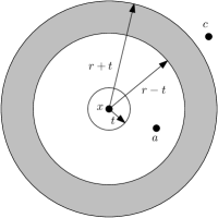
Figure 1: A schematic description of the lower bound in (3). The clusters that are induced by points which lie outside the ball $B_{X}(x,r+t)$, such as $c$, cannot touch the ball $B_{X}(x,t)$. On the other hand, if a point from $B_{X}(x,r-t)$, such as $a$, appeared first in the random order among the points in $B_{X}(x,r+t)$ then its cluster will “swallow” the ball $B_{X}(x,t)$. The probability for this to happen is $\frac{|B(x,r-t)|}{|B(x,r+t)|}$. Only points in the shaded region can split the ball $B_{X}(x,t)$.

Write $\frac{\Delta}{8t}=k+\beta$, where $\beta\in[0,1)$ and $k$ is a positive integer. Then

$$\Pr\left[B_{X}\left(x,t\right)\subseteq\mathscr{P}(x)\right] \geq \frac{4}{\Delta}\int_{\Delta/4}^{\Delta/2}\frac{\left|B_{X}(x,r-t)\right|}{\left|B_{X}(x,r+t)\right|}dr$$

$$= \frac{4}{\Delta}\sum_{j=0}^{k-1}\int_{\frac{\Delta}{4}+2jt}^{\frac{\Delta}{4}+2(j+1)t}\frac{\left|B_{X}(x,r-t)\right|}{\left|B_{X}(x,r+t)\right|}dr+\frac{4}{\Delta}\int_{\frac{\Delta}{4}+2kt}^{\frac{\Delta}{2}}\frac{\left|B_{X}(x,r-t)\right|}{\left|B_{X}(x,r+t)\right|}dr$$

$$\geq \frac{4}{\Delta}\int_{0}^{2t}\sum_{j=0}^{k-1}\frac{\left|B_{X}\left(x,\frac{\Delta}{4}+2jt+s-t\right)\right|}{\left|B_{X}\left(x,\frac{\Delta}{4}+2jt+s+t\right)\right|}ds+\frac{4}{\Delta}\left(\frac{\Delta}{4}-2kt\right)\frac{\left|B_{X}\left(x,\frac{\Delta}{4}+2kt-t\right)\right|}{\left|B_{X}\left(x,\frac{\Delta}{2}+t\right)\right|}$$

$$\geq \frac{4k}{\Delta}\int_{0}^{2t}\left[\prod_{j=0}^{k-1}\frac{\left|B_{X}\left(x,\frac{\Delta}{4}+2jt+s-t\right)\right|}{\left|B_{X}\left(x,\frac{\Delta}{4}+2jt+s+t\right)\right|}\right]^{\frac{1}{k}}ds+\left(1-\frac{8kt}{\Delta}\right)\frac{\left|B_{X}\left(x,\frac{\Delta}{4}+2kt-t\right)\right|}{\left|B_{X}\left(x,\frac{\Delta}{2}+t\right)\right|}$$

$$= \frac{4k}{\Delta}\cdot\int_{0}^{2t}\left[\frac{\left|B_{X}\left(x,\frac{\Delta}{4}+s-t\right)\right|}{\left|B_{X}\left(x,\frac{\Delta}{4}+2t\left(k-1\right)+s+t\right)\right|}\right]^{\frac{1}{k}}ds+\left(1-\frac{8kt}{\Delta}\right)\frac{\left|B_{X}\left(x,\frac{\Delta}{4}+2kt-t\right)\right|}{\left|B_{X}\left(x,\frac{\Delta}{2}+t\right)\right|}$$

$$\geq \frac{8kt}{\Delta}\left[\frac{\left|B_{X}\left(x,\frac{\Delta}{4}-t\right)\right|}{\left|B_{X}\left(x,\frac{\Delta}{4}+2kt+t\right)\right|}\right]^{\frac{1}{k}}+\left(1-\frac{8kt}{\Delta}\right)\frac{\left|B_{X}\left(x,\frac{\Delta}{4}+2kt-t\right)\right|}{\left|B_{X}\left(x,\frac{\Delta}{2}+t\right)\right|}$$

$$\geq \left[\frac{\left|B_{X}\left(x,\frac{\Delta}{4}-t\right)\right|}{\left|B_{X}\left(x,\frac{\Delta}{4}+2kt+t\right)\right|}\right]^{\frac{8t}{\Delta}}\cdot\left[\frac{\left|B_{X}\left(x,\frac{\Delta}{4}+2kt-t\right)\right|}{\left|B_{X}\left(x,\frac{\Delta}{2}+t\right)\right|}\right]^{1-\frac{8kt}{\Delta}}$$

$$= \left[\frac{\left|B_{X}\left(x,\frac{\Delta}{4}-t\right)\right|}{\left|B_{X}\left(x,\frac{\Delta}{4}+2kt+t\right)\right|}\cdot\frac{\left|B_{X}\left(x,\frac{\Delta}{4}+2kt-t\right)\right|}{\left|B_{X}\left(x,\frac{\Delta}{2}+t\right)\right|}\right]^{\frac{8t}{\Delta}}\cdot\left[\frac{\left|B_{X}\left(x,\frac{\Delta}{4}+2kt-t\right)\right|}{\left|B_{X}\left(x,\frac{\Delta}{2}+t\right)\right|}\right]^{\frac{8t}{\Delta}\left(\frac{\Delta}{8t}-k-1\right)}$$

$$\geq \left[\frac{\left|B_{X}\left(x,\frac{\Delta}{4}-t\right)\right|}{\left|B_{X}\left(x,\frac{\Delta}{2}+t\right)\right|}\right]^{\frac{16t}{\Delta}},$$ (7)

where in (3) we used (3), in (3) we used the arithmetic mean/geometric mean inequality, in (3) we used the elementary inequality $\theta a+(1-\theta)b\geq a^{\theta}b^{1-\theta}$, which holds for all $\theta\in[0,1]$ and $a,b\geq 0$, and in (7) we used the fact that $\frac{\Delta}{8t}-k-1$ is negative. ∎

The following theorem, in conjunction with Lemma 2.1, implies Theorem 1.1.

Theorem 3.2.

For every $\alpha>1$, every finite metric space $(X,d_{X})$ admits a completely $1/\alpha$ padded random partition tree with exponent $16/\alpha$.

Proof.

Fix $\alpha>1$. Without loss of generality we may assume that $\operatorname{diam}(X)=1$. We construct a partition tree $\{\mathscr{E}_{k}\}_{k=0}^{\infty}$ of $X$ as follows. Set $\mathscr{E}_{0}=\{X\}$. Having defined $\mathscr{E}_{k}$ we let $\mathscr{P}_{k+1}$ be a partition as in Lemma 3.1 with $\Delta=8^{-k}$ and $t=\Delta/\alpha$ (the random partition $\mathscr{P}_{k+1}$ is chosen independently of the random partitions $\mathscr{P}_{1},\ldots,\mathscr{P}_{k}$). Define $\mathscr{E}_{k+1}$ to be the common refinement of $\mathscr{E}_{k}$ and $\mathscr{P}_{k+1}$, i.e.

$$\mathscr{E}_{k+1}\coloneqq\{C\cap C^{\prime}:\ C\in\mathscr{E}_{k},\ C^{\prime}\in\mathscr{P}_{k+1}\}.$$

The construction implies that for every $x\in X$ and every $k\geq 0$ we have $\mathscr{E}_{k+1}(x)=\mathscr{E}_{k}(x)\cap\mathscr{P}_{k+1}(x)$. Thus one proves inductively that

$$\forall\ k\in\mathbb{N},\ B_{X}\left(x,\frac{8^{-k}}{\alpha}\right)\subseteq\mathscr{P}_{k}(x)\implies\forall\ k\in\mathbb{N},\ B_{X}\left(x,\frac{8^{-k}}{\alpha}\right)\subseteq\mathscr{E}_{k}(x).$$

From Lemma 3.1 and the independence of $\{\mathscr{P}_{k}\}_{k=1}^{\infty}$ it follows that

$$\Pr\left[\forall\ k\in\mathbb{N},\ B_{X}\left(x,\frac{8^{-k}}{\alpha}\right)\subseteq\mathscr{E}_{k}(x)\right] \geq \Pr\left[\forall\ k\in\mathbb{N},\ B_{X}\left(x,\frac{8^{-k}}{\alpha}\right)\subseteq\mathscr{P}_{k}(x)\right]$$

$$= \prod_{k=1}^{\infty}\Pr\left[B_{X}\left(x,\frac{8^{-k}}{\alpha}\right)\subseteq\mathscr{P}_{k}(x)\right]$$

$$\geq \prod_{k=1}^{\infty}\left[\frac{|B_{X}(x,8^{-k-1})|}{|B_{X}(x,8^{-k})|}\right]^{\frac{16}{\alpha}}$$

$$= |B_{X}(x,1/8)|^{-\frac{16}{\alpha}}\geq|X|^{-\frac{16}{\alpha}}.\qed$$

4 Applications to proximity data structures

In this section we show how Theorem 3.2 can be applied to the design of various proximity data structures, which are listed below. Before doing so we shall recall some standard facts about tree representations of ultrametrics, all of which can be found in the discussion in [5]. Any finite ultrametric $(X,\rho)$ can be represented by a rooted tree $T=(V,E)$ with labels $\Delta:V\to(0,\infty)$, whose leaves are $X$, and such that if $u,v\in V$ and $v$ is a child of $u$ then $\Delta(v)\leq\Delta(u)$. Given $x,y\in X$ we then have $\rho(x,y)=\Delta\left(\mathrm{\bf lca}(x,y)\right)$, where $\mathrm{\bf lca}(x,y)$ is the least common ancestor of $x$ and $y$ in $T$. For $k\geq 1$ the labelled tree described above is called a $k$-HST (hierarchically well separated tree) if its labels satisfy the stronger decay condition $\Delta(v)\leq\frac{\Delta(u)}{k}$ whenever $v$ is a child of $u$. The tree $T$ is called an exact $k$-HST if we actually have an equality $\Delta(v)=\frac{\Delta(u)}{k}$ whenever $v$ is a child of $u$. Lemma 3.5 in [5] implies that any $n$-point ultrametric is $k$-equivalent to a metric on $k$-HST which can be computed in time $O(n)$.

We start by proving several structural lemmas which will play a crucial role in the design of our new data structures.

Lemma 4.1 (Extending ultrametrics).

Let $(X,d_{X})$ be a finite metric space, and $\alpha\geq 1$. Fix $\emptyset\neq Y\subseteq X$, and assume that there exits an ultrametric $\rho$ on $Y$ such that for every $x,y\in Y$, $d_{X}(x,y)\leq\rho(x,y)\leq\alpha d_{X}(x,y)$. Then there exists an ultrametric $\widetilde{\rho}$ defined on all of $X$ such that for every $x,y\in X$ we have $d_{X}(x,y)\leq\widetilde{\rho}(x,y)$, and if $x\in X$ and $y\in Y$ then $\widetilde{\rho}(x,y)\leq 6\alpha d_{X}(x,y)$.

Proof.

Let $T=(V,E)$ be the 1-HST representation of $\rho$, with labels $\Delta:V\to(0,\infty)$. In other words, the leaves of $T$ are $Y$, and for every $x,y\in Y$ we have $\Delta(\mathrm{\bf lca}(x,y))=\rho(x,y)$. It will be convenient to augment $T$ by adding an incoming edge to the root with $\Delta(\mathrm{parent}(\mathrm{root}))=\infty$. This clearly does not change the induced metric on $Y$. For every $x\in X\setminus Y$ let $y\in Y$ be its closest point in $Y$, i.e. $d_{X}(x,y)=d_{X}(x,Y)$. Let $u$ be the least ancestor of $y$ for which $\Delta(u)\geq d_{X}(x,y)$ (such a $u$ must exist because we added the incoming edge to the root). Let $v$ be the child of $u$ along the path connecting $u$ and $y$. We add a vertex $w$ on the edge $\{u,v\}$ whose label is $d_{X}(x,y)$, and connect $x$ to $T$ as a child of $w$. The resulting tree is clearly still a $1$-HST. Repeating this procedure for every $x\in X\setminus Y$ we obtain a $1$-HST $\widetilde{T}$ whose leaves are $X$. Denote the labels on $\widetilde{T}$ by $\widetilde{\Delta}$.

Fix $x,y\in X$, and let $x^{\prime},y^{\prime}\in Y$ the nearest neighbors of $x,y$ (respectively) used in the above construction. Then

$$\widetilde{\Delta}\left(\mathrm{\bf lca}_{\widetilde{T}}(x,y)\right) = \max\left\{\widetilde{\Delta}\left(\mathrm{\bf lca}_{\widetilde{T}}(x,x^{\prime})\right),\widetilde{\Delta}\left(\mathrm{\bf lca}_{\widetilde{T}}(y,y^{\prime})\right),\widetilde{\Delta}\left(\mathrm{\bf lca}_{\widetilde{T}}(x^{\prime},y^{\prime})\right)\right\}$$ (8)

$$\geq \max\left\{d_{X}(x,x^{\prime}),d_{X}(y,y^{\prime}),d_{X}(x^{\prime},y^{\prime})\right\}$$

$$\geq \frac{d_{X}(x,x^{\prime})+d_{X}(y,y^{\prime})+d_{X}(x^{\prime},y^{\prime})}{3}$$

$$\geq \frac{1}{3}\,d_{X}(x,y).$$

In the reverse direction, if $x\in X$ and $y\in Y$ let $x^{\prime}\in Y$ be the closest point in $Y$ to $x$ used in the construction of $\widetilde{T}$. Then $d_{X}(x^{\prime},y)\leq d_{X}(x^{\prime},x)+d_{X}(x,y)\leq 2d_{X}(x,y)$. If $\mathrm{\bf lca}_{\widetilde{T}}(y,x^{\prime})$ is an ancestor of $\mathrm{\bf lca}_{\widetilde{T}}(x,x^{\prime})$ then

$$\widetilde{\Delta}\left(\mathrm{\bf lca}_{\widetilde{T}}(x,y)\right)=\widetilde{\Delta}\left(\mathrm{\bf lca}_{\widetilde{T}}(x^{\prime},y)\right)=\rho(x^{\prime},y)\leq\alpha\cdot d_{X}(x^{\prime},y)\leq 2\alpha\cdot d_{X}(x,y).$$ (9)

If, on the other hand, $\mathrm{\bf lca}_{\widetilde{T}}(y,x^{\prime})$ is a descendant of $\mathrm{\bf lca}_{\widetilde{T}}(x,x^{\prime})$ then

$$\widetilde{\Delta}\left(\mathrm{\bf lca}_{\widetilde{T}}(x,y)\right)=\widetilde{\Delta}\left(\mathrm{\bf lca}_{\widetilde{T}}(x,x^{\prime})\right)=d_{X}(x,x^{\prime})\leq d_{X}(x,y).$$ (10)

Scaling the labels of $\widetilde{T}$ by a factor of $3$, the required result is a combination of (8), (9) and (10). ∎

The following lemma is a structural result on the existence of a certain distribution over decreasing chains of subsets of a finite metric space. In what follows we shall call such a distribution a stochastic Ramsey chain. A schematic description of this notion, and the way it is used in the ensuing arguments, is presented in Figure 2 below.

Lemma 4.2 (Stochastic Ramsey chains).

Let $(X,d_{X})$ be an $n$-point metric space and $k\geq 1$. Then there exists a distribution over decreasing sequences of subsets $X=X_{0}\supsetneqq X_{1}\supsetneqq X_{2}\cdots\supsetneqq X_{s}=\emptyset$ ($s$ itself is a random variable), such that for all $p>-1/k$,

$$\mathbb{E}\left[\sum_{j=0}^{s-1}|X_{j}|^{p}\right]\leq\left(\max\left\{\frac{k}{1+pk},1\right\}\right)\cdot n^{p+1/k},$$ (11)

and such that for each $j\in\{1,\ldots,s\}$ there exists an ultrametric $\rho_{j}$ on $X$ satisfying for every $x,y\in X$, $\rho_{j}(x,y)\geq d_{X}(x,y)$, and if $x\in X$ and $y\in X_{j-1}\setminus X_{j}$ then $\rho_{j}(x,y)\leq O(k)\cdot d_{X}(x,y)$.

Remark 4.1.

In what follows we will only use the cases $p\in\{0,1,2\}$ in Lemma 4.2. Observe that for $p=0$, (11) is simply the estimate $\mathbb{E}s\leq kn^{1/k}$.

Proof of Lemma 4.2.

By Theorem 3.2 and the proof of Lemma 2.1 there is a distribution over subsets $Y_{1}\subseteq X_{0}$ such that $\mathbb{E}|Y_{1}|\geq n^{1-1/k}$ and there exists an ultrametric $\rho_{1}$ on $Y_{1}$ such that every $x,y\in Y_{1}$ satisfy $d_{X}(x,y)\leq\rho_{1}(x,y)\leq O(k)\cdot d_{X}(x,y)$. By Lemma 4.1 we may assume that $\rho_{1}$ is defined on all of $X$, for every $x,y\in X$ we have $\rho_{1}(x,y)\geq d_{X}(x,y)$, and if $x\in X$ and $y\in Y_{1}$ then $\rho_{1}(x,y)\leq O(k)\cdot d_{X}(x,y)$. Define $X_{1}=X_{0}\setminus Y_{1}$ and apply the same reasoning to $X_{1}$, obtaining a random subset $Y_{2}\subseteq X_{0}\setminus Y_{1}$ and an ultrametric $\rho_{2}$. Continuing in this manner until we arrive at the empty set, we see that there are disjoint subsets, $Y_{1},\ldots,Y_{s}\subseteq X$, and for each $j$ an ultrametric $\rho_{j}$ on $X$, such that for $x,y\in X$ we have $\rho_{j}(x,y)\geq d_{X}(x,y)$, and for $x\in X$, $y\in Y_{j}$ we have $\rho_{j}(x,y)\leq O(k)\cdot d_{X}(x,y)$. Additionally, writing $X_{j}\coloneqq X\setminus\bigcup_{i=1}^{j}Y_{i}$, we have the estimate $\mathbb{E}\left[|Y_{j}|\Big{|}Y_{1},\ldots,Y_{j-1}\right]\geq|X_{j-1}|^{1-1/k}$.

The proof of (11) is by induction on $n$. For $n=1$ the claim is obvious, and if $n>1$ then by the inductive hypothesis

$$\mathbb{E}\left[\left.\sum_{j=0}^{s-1}|X_{j}|^{p}\right|Y_{1}\right] \leq n^{p}+\left(\max\left\{\frac{k}{1+pk},1\right\}\right)\cdot|X_{1}|^{p+1/k}$$

$$= n^{p}+\left(\max\left\{\frac{k}{1+pk},1\right\}\right)\cdot n^{p+1/k}\left(1-\frac{|Y_{1}|}{n}\right)^{p+1/k}$$

$$\leq n^{p}+\left(\max\left\{\frac{k}{1+pk},1\right\}\right)\cdot n^{p+1/k}\left(1-\left(\min\left\{p+\frac{1}{k},1\right\}\right)\cdot\frac{|Y_{1}|}{n}\right)$$

$$= \left(\max\left\{\frac{k}{1+pk},1\right\}\right)\cdot n^{p+1/k}+n^{p}-n^{p-1+1/k}|Y_{1}|.$$

Taking expectation with respect to $Y_{1}$ gives the required result. ∎

Observation 4.3.

If one does not mind losing a factor of $O(\log n)$ in the construction time and storage of the Ramsey chain, then an alternative to Lemma 4.2 is to randomly and independently sample $O\left(n^{1/k}\log n\right)$ ultrametrics from the Ramsey partitions.

Before passing to the description of our new data structures, we need to say a few words about the algorithmic implementation of Lemma 4.2 (this will be the central preprocessing step in our constructions). The computational model in which we will be working is the RAM model, which is standard in the context of our type of data-structure problems (see for example [32]). In fact, we can settle for weaker computational models such as the “Unit cost floating-point word RAM model” — a detailed discussion of these issues can be found in Section 2.2. of [20].

The natural implementation of the Calinescu-Karloff-Rabani (CKR) random partition used in the proof of Lemma 3.1 takes $O\left(n^{2}\right)$ time. Denote by $\Phi=\Phi(X)$ the aspect ratio of $X$, i.e. the diameter of $X$ divided by the minimal positive distance in $X$. The construction of the distribution over partition trees in the proof of Theorem 3.2 requires performing $O(\log\Phi)$ such decompositions. This results in $O\left(n^{2}\log\Phi\right)$ preprocessing time to sample one partition tree from the distribution. Using a standard technique (described for example in [20, Sections 3.2-3.3]), we dispense with the dependence on the aspect ratio and obtain that the expected preprocessing time of one partition tree is $O\left(n^{2}\log n\right)$. Since the argument in [20] is presented in a slightly different context, we shall briefly sketch it here.

We start by constructing an ultrametric $\rho$ on $X$, represented by an HST $H$, such that for every $x,y\in X$, $d_{X}(x,y)\leq\rho(x,y)\leq nd_{X}(x,y)$. The fact that such a tree exists is contained in [5, Lemma 3.6], and it can be constructed in time $O\left(n^{2}\right)$ using the Minimum Spanning Tree algorithm. This implementation is done in [20, Section 3.2]. We then apply the CKR random partition with diameter $\Delta$ as follows: Instead of applying it to the points in $X$, we apply it to the vertices $u$ of $H$ for which

$$\Delta(u)\leq\frac{\Delta}{n^{2}}<\Delta\left(\mathrm{parent}(u)\right).$$ (12)

Each such vertex $u$ represents all the subtree rooted at $u$ (in particular, we can choose arbitrary leaf descendants to calculate distances — these distances are calculated using the metric $d_{X}$), and they are all assigned to the same cluster as $u$ in the resulting partition. This is essentially an application of the algorithm to an appropriate quotient of $X$ (see the discussion in [27]). We actually apply a weighted version of the CKR decomposition in the spirit of [25], in which, in the choice of random permutation, each vertex $u$ as above is chosen with probability proportional to the number of leaves which are descendants of $u$ (note that this change alters the guarantee of the partition only slightly: We will obtain clusters bounded by $\left(1+1/n^{2}\right)\Delta$, and in the estimate on the padding probability the radii of the balls is changed by only a factor of $(1\pm 1/n)$). We also do not process each scale, but rather work in “event driven mode”: Vertices of $H$ are put in a non decreasing order according to their labels in a queue. Each time we pop a new vertex $u$, and partition the spaces at all the scales in the range $[\Delta(u),n^{2}\Delta(u)]$, for which we have not done so already. In doing so we effectively skip “irrelevant” scales. To estimate the running time of this procedure note that the CKR decomposition at scale $8^{j}$ takes time $O\left(m_{i}^{2}\right)$, where $m_{i}$ is the number of vertices $u$ of $H$ satisfying (12) with $\Delta=8^{i}$. Note also that each vertex of $H$ participates in at most $O(\log n)$ such CKR decompositions, so $\sum_{i}m_{i}=O(n\log n)$. Hence the running time of the sampling procedure in Lemma 4.2 is up to a constant factor $\sum_{i}m_{i}^{2}=O\left(n^{2}\log n\right)$.

The Ramsey chain in Lemma 4.2 will be used in two different ways in the ensuing constructions. For our approximate distance oracle data structure we will just need that the ultrametric $\rho_{j}$ is defined on $X_{j-1}$ (and not all of $X$). Thus, by the above argument, and Lemma 4.2, the expected preprocessing time in this case is $O\left(\mathbb{E}\sum_{j=1}^{s-1}|X_{j}|^{2}\log|X_{j}|\right)=O\left(n^{2+1/k}\log n\right)$  and the expected storage space is $O\left(\mathbb{E}\sum_{j=1}^{s-1}|X_{j}|\right)=O\left(n^{1+1/k}\right)$. For the purpose of our approximate ranking data structure we will really need the metrics $\rho_{j}$ to be defined on all of $X$. Thus in this case the expected preprocessing time will be $O\left(n^{2}\log n\cdot\mathbb{E}s\right)=O\left(kn^{2+1/k}\log n\right)$, and the expected storage space is $O\left(n\cdot\mathbb{E}s\right)=O\left(kn^{1+1/k}\right)$.

1) Approximate distance oracles.

Our improved approximate distance oracle is contained in Theorem 1.2, which we now prove.

Proof of Theorem 1.2.

We shall use the notation in the statement of Lemma 4.2. Let $T_{j}=(V_{j},E_{j})$ and $\Delta_{j}:V_{j}\to(0,\infty)$ be the HST representation of the ultrametric $\rho_{j}$ (which was actually constructed explicitly in the proofs of Lemma 2.1 and Lemma 4.2). The usefulness of the tree representation stems from the fact that it very easy to handle algorithmically. In particular there exists a simple scheme that takes a tree and preprocesses it in linear time so that it is possible to compute the least common ancestor of two given nodes in constant time (see [21, 6]). Hence, we can preprocess any $1$-HST so that the distance between every two points can be computed in $O(1)$ time.

For every point $x\in X$ let $i_{x}$ be the largest index for which $x\in X_{i_{x}-1}$. Thus, in particular, $x\in Y_{i_{x}}$. We further maintain for every $x\in X$ a vector (in the sense of data-structures) $\mathbf{vec}_{x}$ of length $i_{x}$ (with $O(1)$ time direct access), such that for $i\in\{0,\ldots,i_{x}-1\}$, $\mathbf{vec}_{x}[i]$ is a pointer to the leaf representing $x$ in $T_{i}$. Now, given a query $x,y\in X$ assume without loss of generality that $i_{x}\leq i_{y}$. It follows that $x,y\in X_{i_{x}-1}$. We locate the leaves $\hat{x}=\mathbf{vec}_{x}[i_{x}]$, and $\hat{y}=\mathbf{vec}_{y}[i_{x}]$ in $T_{i_{x}}$, and then compute $\Delta(\mathbf{lca}\left(\hat{x},\hat{y}\right))$ to obtain an $O(k)$ approximation to $d_{X}(x,y)$. Observe that the above data structure only requires $\rho_{j}$ to be defined on $X_{j-1}$ (and satisfying the conclusion of Lemma 4.2 for $x,y\in X_{j-1}$). The expected preprocessing time is $O\left(n^{2+1/k}\log n\right)$. The size of the above data structure is $O\left(\sum_{j=0}^{s}|X_{j}|\right)$, which is in expectation $O\left(n^{1+1/k}\right)$. ∎

Remark 4.2.

Using the distributed labeling for the least common ancestor operation on trees of Peleg [29], the procedure described in the proof of Theorem 1.2 can be easily converted to a distance labeling data structure (we refer to [32, Section 3.5] for a description of this problem). We shall not pursue this direction here, since while the resulting data structure is non-trivial, it does not seem to improve over the known distance labeling schema [32].

Figure 2: A schematic description of Ramsey chains and the way they are used to construct approximate distance oracles and approximate ranking data structures. Ramsey chains are obtained by iteratively applying Theorem 3.2 and Lemma 2.1 to find a decreasing chain of subsets $X=X_{0}\supsetneqq X_{1}\supsetneqq X_{2}\cdots\supsetneqq X_{s}=\emptyset$ such that $X_{j}$ can be approximated by a tree metric $T_{j+1}$. The tree $T_{j+1}$ is, in a sense, a “distance estimator” for $X_{j}\setminus X_{j+1}$ — it can be used to approximately evaluate the distance from a point in $X_{j}\setminus X_{j+1}$ to any other point in $X_{j}$. These trees form an array which is an approximate distance oracle. In the case of approximate ranking we also need to extend the tree $T_{j+1}$ to a tree on the entire space $X$ using Lemma 4.1. The nodes that were added to these trees are illustrated by empty circles, and the dotted lines are their connections to the original tree.

2) Approximate ranking.

Before proceeding to our $\alpha$-approximate ranking data structure (Theorem 1.3) we recall the setting of the problem. Thinking of $X$ as a metric on $\{1,\ldots,n\}$, and fixing $\alpha>1$, the goal here is to associate with every $x\in X$ a permutation $\pi^{(x)}$ of $\{1,\ldots,n\}$ such that $d_{X}\bigl{(}x,\pi^{(x)}(i)\bigr{)}\leq\alpha\cdot d_{X}\bigl{(}x,\pi^{(x)}(j)\bigr{)}$ for every $1\leq i\leq j\leq n$. This relaxation of the exact proximity ranking induced by the metric $d_{X}$ allows us to gain storage efficiency, while enabling fast access to this data. By fast access we mean that we can preform the following tasks:

1. Given an element $x\in X$, and $i\in\{1,\ldots,n\}$, find $\pi^{(x)}(i)$ in $O(1)$ time.

2. Given an element $x\in X$ and $y\in X$, find number $i\in\{1,\ldots,n\}$, such that $\pi^{(x)}(i)=y$, in $O(1)$ time.

We also require the following lemma.

Lemma 4.4.

Let $T=(V,E)$ be a rooted tree with $n$ leaves. For $v\in V$, let $\mathscr{L}_{T}(v)$ be the set of leaves in the subtree rooted at $v$, and denote $\ell_{T}(v)=\left|\mathscr{L}_{T}(v)\right|$. Then there exists a data structure, that we call Size-Ancestor, which can be constructed in time $O(n)$, so as to answer in time $O(1)$ the following query: Given $\ell\in\mathbb{N}$ and a leaf $x\in V$, find an ancestor $u$ of $x$ such that $\ell_{T}(u)<\ell\leq\ell(\mathrm{parent}(u))$. Here we use the convention $\ell(\mathrm{parent}(\mathrm{root}))=\infty$.

To the best of our knowledge, the data structure described in Lemma 4.4 has not been previously studied. We therefore include a proof of Lemma 4.4 in Appendix A, and proceed at this point to conclude the proof of Theorem 1.3.

Proof of Theorem 1.3.

We shall use the notation in the statement of Lemma 4.2. Let $T_{j}=(V_{j},E_{j})$ and $\Delta_{j}:V_{j}\to(0,\infty)$ be the HST representation of the ultrametric $\rho_{j}$. We may assume without loss of generality that each of these trees is binary and does not contain a vertex which has only one child. Before presenting the actual implementation of the data structure, let us explicitly describe the permutation $\pi^{(x)}$ that the data structure will use. For every internal vertex $v\in V_{j}$ assign arbitrarily the value $0$ to one of its children, and the value $1$ to the other. This induces a unique (lexicographical) order on the leaves of $T_{j}$. Next, fix $x\in X$ and $i_{x}$ such that $x\in Y_{i_{x}}$. The permutation $\pi^{(x)}$ is defined as follows. Starting from the leaf $x$ in $T_{i_{x}}$, we scan the path from $x$ to the root of $T_{i_{x}}$. On the way, when we reach a vertex $u$ from its child $v$, let $w$ denote the sibling of $v$, i.e. the other child of $u$. We next output all the leafs which are descendants of $w$ according to the total order described above. Continuing in this manner until we reach the root of $T_{i_{x}}$ we obtain a permutation $\pi^{(x)}$ of $X$.

We claim that the permutation $\pi^{(x)}$ constructed above is an $O(k)$-approximation to the proximity ranking induced by $x$. Indeed, fix $y,z\in X$ such that $Ck\cdot d_{X}(x,y)<d_{X}(x,z)$, where $C$ is a large enough absolute constant. We claim that $z$ will appear after $y$ in the order induced by $\pi^{(x)}$. This is true since the distances from $x$ are preserved up to a factor of $O(k)$ in the ultrametric $T_{i_{x}}$. Thus for large enough $C$ we are guaranteed that $d_{T_{i_{x}}}(x,y)<d_{T_{i_{x}}}(x,z)$, and therefore $\mathrm{\bf lca}_{T_{i_{x}}}(x,z)$ is a proper ancestor of $\mathrm{\bf lca}_{T_{i_{x}}}(x,y)$. Hence in the order just describe above, $y$ will be scanned before $z$.

We now turn to the description of the actual data structure, which is an enhancement of the data structure constructed in the proof of Theorem 1.2. As in the proof of Theorem 1.2 our data structure will consist of a “vector of the trees $T_{j}$”, where we maintain for each $x\in X$ a pointer to the leaf representing $x$ in each $T_{j}$. The remaining description of our data structure will deal with each tree $T_{j}$ separately. First of all, with each vertex $v\in T_{j}$ we also store the number of leaves which are the descendants of $v$, i.e. $|\mathscr{L}_{T_{j}}(v)|$ (note that all these numbers can be computed in $O(n)$ time using, say, depth-first search). With each leaf of $T_{j}$ we also store its index in the order described above. There is a reverse indexing by a vector for each tree $T_{j}$ that allows, given an index, to find the corresponding leaf of $T_{j}$ in $O(1)$ time. Each internal vertex contains a pointer to its leftmost (smallest) and rightmost (largest) descendant leaves. This data structure can be clearly constructed in $O(n)$ time using, e.g., depth-first transversal of the tree. We now give details on how to answer the required queries using the “ammunition” we have listed above.

1. Using Lemma 4.4, find an ancestor $v$ of $x$ such that $\ell_{T_{j}}(v)<i\leq\ell_{T_{j}}(\text{parent}(v))$ in $O(1)$ time. Let $u=\text{parent}(v)$ (note that $v$ can not be the root). Let $w$ be the sibling of $v$ (i.e. the other child of $u$). Next we pick the leaf numbered $\left(i-\ell_{T_{j}}(v)\right)+\text{left}(w)-1$, where $\text{left}(w)$ is the index to the leftmost descendant of $w$.

2. Find $u=\mathrm{\bf lca}(x,y)$ (in $O(1)$ time, using [21, 6]). Let $v$ and $w$ be the children of $u$, which are ancestors of $x$ and $y$, respectively. Return $\ell_{T_{j}}(v)+\text{ind}(y)-\text{left}(w)$, where $\text{ind}(y)$ is the index of $y$ in the total order of the leaves of the tree.

This concludes the construction of our approximate ranking data structure. Because we need to have the ultrametric $\rho_{j}$ defined on all of $X$, the preprocessing time is $O\left(kn^{2+1/k}\log n\right)$ and the storage size is $O\left(kn^{1+1/k}\right)$, as required. ∎

Remark 4.3.

Our approximate ranking data structure can also be used in a nearest neighbor heuristic called “Orchard Algorithm” [28] (see also [13, Sec. 3.2]). In this algorithm the vanilla heuristic can be used to obtain the exact proximity ranking, and requires storage $\Omega\left(n^{2}\right)$. Using approximate ranking the storage requirement can be significantly improved, though the query performance is somewhat weaker due to the inaccuracy of the ranking lists.

3) Computing the Lipschitz constant.

Here we describe a data structure for computing the Lipschitz constant of a function $f:X\to Y$, where $(Y,d_{Y})$ is an arbitrary metric space. When $(X,d_{X})$ is a doubling metric space (see [22]), this problem was studied in [20]. In what follows we shall always assume that $f$ is given in oracle form, i.e. it is encoded in such a way that we can compute its value on a given point in constant time.

Lemma 4.5.

There is an algorithm that, given an $n$-point ultrametric $(U,d_{U})$ defined by the HST $T=(V,E)$ (in particular $U$ is the set of leaves of $T$), an arbitrary metric space $(Y,d_{Y})$, and a mapping $f:U\to Y$, returns in time $O(n)$ a number $A\geq 0$ satisfying $\|f\|_{\mathrm{Lip}}\geq A\geq\frac{1}{16}\cdot\|f\|_{\mathrm{Lip}}$.

Proof.

We assume that $T$ is 4-HST. As remarked in the beginning of Section 4, this can be achieved by distorting the distances in $U$ by a factor of at most $4$, in $O(n)$ time. We also assume that the tree $T$ stores for every vertex $v\in V$ an arbitrary leaf $x_{v}\in U$ which is a descendant of $v$ (this can be easily computed in $O(n)$ time). For a vertex $u\in V$ we denote by $\Delta(u)$ its label (i.e. $\forall\ x,y\in U,\ d_{U}(x,y)=\Delta(\mathrm{\bf lca}(x,y))$).

The algorithm is as follows:

       Lip-UM$(T,f)$ $A\leftarrow 0$ For every vertex $u\in T$ do Let $v_{1},\ldots v_{r}$ be the children of $u$. $A\leftarrow\max\left\{A,\max_{2\leq i\leq r}\frac{d_{Y}\left(f(x_{v_{1}}),f(x_{v_{i}})\right)}{\Delta(u)}\right\}$ Output $A$.

Clearly the algorithm runs in linear time (the total number of vertices in the tree is $O(n)$ and each vertex is visited at most twice). Furthermore, by construction the algorithm outputs $A\leq\|f\|_{\text{Lip}}$. It remains to prove a lower bound on $A$. Let $x_{1},x_{2}\in U$ be such that $\|f\|_{\text{Lip}}=\frac{d_{Y}(f(x_{1}),f(x_{2}))}{d_{U}(x_{1},x_{2})}$, and denote $u=\mathrm{\bf lca}(x,y)$. Let $w_{1},w_{2}$ be the children of $u$ such that $x_{1}\in\mathscr{L}_{T}(w_{1})$, and $x_{2}\in\mathscr{L}_{T}(w_{2})$. Let $v_{1}$ be the “first child” of $u$ as ordered by the algorithm Lip-UM (notice that this vertex has special role). Then

$$A \geq \max\left\{\frac{d_{Y}(f(x_{w_{1}}),f(x_{v_{1}}))}{\Delta(u)},\frac{d_{Y}(f(x_{w_{2}}),f(x_{v_{1}}))}{\Delta(u)}\right\}$$

$$\geq \frac{1}{2}\cdot\frac{d_{Y}(f(x_{w_{1}}),f(x_{w_{2}}))}{\Delta(u)}$$

$$\geq \frac{1}{2}\cdot\frac{d_{Y}(f(x_{1}),f(x_{2}))-\operatorname{diam}(f(\mathscr{L}_{T}(w_{1})))-\operatorname{diam}(f(\mathscr{L}_{T}(w_{2})))}{\Delta(u)}.$$

If $\max\left\{\operatorname{diam}(f(\mathscr{L}_{T}(w_{1}))),\operatorname{diam}(f(\mathscr{L}_{T}(w_{2})))\right\}\leq\frac{1}{4}d_{Y}(f(x_{1}),f(x_{2}))$, then we conclude that

$$A\geq\frac{1}{4}\cdot\frac{d_{Y}(f(x_{1}),f(x_{2}))}{\Delta(u)},$$

as needed. Otherwise, assuming that $\operatorname{diam}(f(\mathscr{L}_{T}(w_{1})))>\frac{1}{4}\cdot d_{Y}(f(x_{1}),f(x_{2}))$, there exist $z,z^{\prime}\in\mathscr{L}_{T}(w_{1})$ such that

$$\frac{d_{Y}(f(z),f(z^{\prime}))}{d_{U}(z,z^{\prime})}>\frac{\frac{1}{4}\cdot d_{Y}(f(x_{1}),f(x_{2}))}{\Delta(u)/4}=\|f\|_{\text{Lip}},$$

which is a contradiction. ∎

Theorem 4.6.

Given $k\geq 1$, any $n$-point metric space $(X,d_{X})$ can be preprocessed in time $O\left(n^{2+1/k}\log n\right)$, yielding a data structure requiring storage $O\left(n^{1+1/k}\right)$ which can answer in $O\left(n^{1+1/k}\right)$ time the following query: Given a metric space $(Y,d_{Y})$ and a mapping $f:X\to Y$, compute a value $A\geq 0$, such that $\|f\|_{\mathrm{Lip}}\geq A\geq\|f\|_{\mathrm{Lip}}/O(k)$.

Proof.

The preprocessing is simply computing the trees $\{T_{j}\}_{j=1}^{s}$ as in the proof of Theorem 1.2. Denote the resulting ultrametrics by $(U_{1},\rho_{1}),\ldots,(U_{s},\rho_{s})$. Given $f:X\to Y$, represent it as $g_{i}:U_{i}\to Y$ (as a mapping $g_{i}$ is the same mapping as the restriction of $f$ to $U_{i}$). Use Lemma 4.5 to compute an estimate $A_{i}$ of $\|g_{i}\|_{\mathrm{Lip}}$, and return $A\coloneqq\max_{i}A_{i}$. Since all the distances in $U_{i}$ dominate the distances in $X$, $\|f\|_{\mathrm{Lip}}\geq\|g_{i}\|_{\mathrm{Lip}}\geq A_{i}$, so $\|f\|_{\mathrm{Lip}}\geq A$. On the other hand, let $x,y\in X$ be such that $\|f\|_{\mathrm{Lip}}=\frac{d_{Y}(f(x),f(y))}{d_{X}(x,y)}$. By Lemma 4.2, there exists $i\in\{1,\ldots,s\}$ such that $d_{U_{i}}(x,y)\leq O(k)\cdot d_{X}(x,y)$, and hence $\|g_{i}\|_{\mathrm{Lip}}\geq\|f\|_{\mathrm{Lip}}/O(k)$, And so $A\geq\frac{1}{16}\cdot\|g_{i}\|_{\mathrm{Lip}}\geq\|f\|_{\mathrm{Lip}}/O(k)$, as required. Since we once more only need that the ultrametric $\rho_{j}$ is defined on $X_{j-1}$ and not on all of $X$, the preprocessing time and storage space are the same as in Theorem 1.2. By Lemma 4.2 the query time is $O\left(\sum_{j=1}^{s-1}|X_{j}|\right)=O\left(n^{1+1/k}\right)$ (we have a $O(|X_{j}|)$ time computation of the Lipschitz constant on each $X_{j}$). ∎

5 Concluding Remarks

An $s$-well separated pair decomposition (WSPD) of an $n$-point metric space $(X,d_{X})$ is a collection of pair of subsets $\{(A_{i},B_{i})\}_{i=1}^{M}$, $A_{i},B_{i}\subset X$, such that

1. $\forall x,y\in X$ if $x\neq y$ then $(x,y)\in\bigcup_{i=1}^{M}(A_{i}\times B_{i})$.

2. For all $i\neq j$, $(A_{i}\times B_{i})\cap(A_{j}\times B_{j})=\emptyset$.

3. For all $i\in\{1,\ldots,M\}$, $d_{X}(A_{i},B_{i})\geq s\cdot\max\{\operatorname{diam}(A_{i}),\operatorname{diam}(B_{i})\}$.

The notion of $s$-WSPD was first defined for Euclidean spaces in an influential paper of Callahan and Kosaraju [11], where it was shown that for $n$-point subsets of a fixed dimensional Euclidean space there exists such a collection of size $O(n)$ that can be constructed in $O(n\log n)$ time. Subsequently, this concept has been used in many geometric algorithms (e.g. [33, 10]), and is today considered to be a basic tool in computational geometry. Recently the definition and the efficient construction of WSPD were generalized to the more abstract setting of doubling metrics [31, 20]. These papers have further demonstrated the usefulness of this tool (see also [18] for a mathematical application).

It would be clearly desirable to have a notion similar to WSPD in general metrics. However, as formulated above, no non-trivial WSPD is possible in “high dimensional” spaces, since any $2$-WSPD of an $n$-point equilateral space must be of size $\Omega(n^{2})$. The present paper suggests that Ramsey partitions might be a partial replacement of this notion which works for arbitrary metric spaces. Indeed, among the applications of WSPD in fixed dimensional metrics are approximate ranking (though this application does not seem to have appeared in print — it was pointed out to us by Sariel Har-Peled), approximate distance oracles [19, 20], spanners [31, 20], and computation of the Lipschitz constant [20]. These applications have been obtained for general metrics using Ramsey partitions in the present paper (spanners were not discussed here since our approach does not seem to beat previously known constructions). We believe that this direction deserves further scrutiny, as there are more applications of WSPD which might be transferable to general metrics using Ramsey partitions. With is in mind it is worthwhile to note here that our procedure for constructing stochastic Ramsey chains, as presented in Section 4, takes roughly $n^{2+1/k}$ time (up to logarithmic terms). For applications it would be desirable to improve this construction time to $O(n^{2})$. The construction time of ceratin proximity data structures is a well studied topic in the computer science literature — see for example [34, 30].

Acknowledgments.

Part of this work was carried out while Manor Mendel was visiting Microsoft Research. We are grateful to Sariel Har-Peled for letting us use here his insights on the approximate ranking problem. We also thank Yair Bartal for helpful discussions.

Appendices

Appendix A The Size-Ancestor data structure

In this appendix we prove Lemma 4.4. Without loss of generality we assume that the tree $T$ does not contain vertices with only one child. Indeed, such vertices will never be returned as an answer for a query, and thus can be eliminated in $O(n)$ time in a preprocessing step.

Our data structure is composed in a modular way of two different data structures, the first of which is described in the following lemma, while the second is discussed in the proof of Lemma 4.4 that will follow.

Lemma A.1.

Fix $m\in\mathbb{N}$, and let $T$ be as in Lemma 4.4. Then there exists a data structure which can be preprocessed in time $O\left(n+\frac{n\log n}{m}\right)$, and answers in time $O(1)$ the following query: Given $\ell\in\mathbb{N}$ and a leaf $x\in V$, find an ancestor $u$ of $x$ such that $\ell_{T}(u)<\ell m\leq\ell(\mathrm{parent}(u))$. Here we use the convention $\ell(\mathrm{parent}(\mathrm{root}))=\infty$.

Proof.

Denote by $X$ the set of leaves of $T$. For every internal vertex $v\in V$, order its children non-increasingly according to the number of leaves in the subtrees rooted at them. Such a choice of labels induces a unique total order on $X$ (the lexicographic order). Denote this order by $\preccurlyeq$ and let $f:\{1,\ldots,n\}\to X$ be the unique increasing map in the total order $\preccurlyeq$. For every $v\in V$, $f^{-1}\left(\mathscr{L}_{T}(v)\right)$ is an interval of integers. Moreover, the set of intervals $\bigl{\{}f^{-1}(\mathscr{L}_{T}(v)):\ v\in V\bigr{\}}$ forms a laminar set, i.e. for every pair of intervals in this set either one is contained in the other, or they are disjoint. For every $v\in V$ write $f^{-1}\left(\mathscr{L}_{T}(v)\right)=I_{v}=[A_{v},B_{v}]$, where $A_{v},B_{v}\in\mathbb{N}$ and $A_{v}\leq B_{v}$. For $i\in\{1,\ldots,\lfloor n/m\rfloor\}$ and $j\in\{1,\ldots,\lceil n/(im)\rceil\}$ let $F_{i}(j)$ be the set of vertices $v\in V$ such that $|I_{v}|\geq im$, $I_{v}\cap[(j-1)im+1,jim]\neq\emptyset$, and there is no descendant of $v$ satisfying these two conditions. Since at most two disjoint intervals of length at least $im$ can intersect a given interval of length $im$, we see that for all $i,j$, $|F_{i}(j)|\leq 2$.

Claim A.2.

Let $x\in X$ be a leaf of $T$, and $\ell\in\mathbb{N}$. Let $u\in V$ be the least ancestor of $x$ for which $\ell_{T}(u)\geq\ell m$. Then

$$u\in\left\{\mathrm{\bf lca}(x,v):\ v\in F_{\ell}\left(\left\lceil\frac{f(x)}{\ell m}\right\rceil\right)\right\}.$$

Proof.

If $u\in F_{\ell}\left(\left\lceil\frac{f(x)}{\ell m}\right\rceil\right)$ then since $u=\mathrm{\bf lca}(x,u)$ there is nothing to prove. If on the other hand $u\notin F_{\ell}\left(\left\lceil\frac{f(x)}{\ell m}\right\rceil\right)$ then since we are assuming that $\ell_{T}(u)\geq\ell m$, and $I_{u}\cap\left[\left(\left\lceil\frac{f(x)}{\ell m}\right\rceil-1\right)\ell m+1,\left\lceil\frac{f(x)}{\ell m}\right\rceil\ell m\right]\neq\emptyset$ (because $f(x)\in I_{u}$), it follows that $u$ has a descendant $v$ in $F_{\ell}\left(\left\lceil\frac{f(x)}{\ell m}\right\rceil\right)$. Thus $u=\mathrm{\bf lca}(x,v)$, by the fact that any ancestor $w$ of $v$ satisfies $\ell_{T}(w)\geq\ell_{T}(v)\geq\ell m$, and the minimality of $u$. ∎

The preprocessing of the data structure begins with ordering the children of vertices non-increasingly according to the number of leaves in their subtrees. The following algorithm achieves it in linear time.

             SORT-CHILDREN$(u)$ Compute $\{\ell_{T}(u)\}_{u\in V}$ using depth first search. Sort $V$ non-increasingly according to $\ell_{T}(\cdot)$ (use bucket sort- see [15, Ch. 9]). Let $(v_{i})_{i}$ be the set $V$ sorted as above. Initialize $\forall u\in V$, the list $\mathsf{ChildrenSortedList}_{u}=\emptyset$. For $i=1$ to $|V|$ do Add $v_{i}$ to the end of $\mathsf{ChildrenSortedList}_{\mathrm{parent}(v_{i})}$.

Computing $f$, and the intervals $\{I_{u}\}_{u\in V}$ is now done by a depth first search of $T$ that respects the above order of the children. We next compute $\left\{F_{i}(j):\ i\in\{1,\ldots,\lfloor n/m\rfloor\},\ j\in\{1,\ldots,\lceil n/(im)\rceil\right\}$ using the following algorithm:

          SUBTREE-COUNT$(u)$ Let $v_{1},\ldots,v_{r}$ be the children of $u$ with $|I_{v_{1}}|\geq|I_{v_{2}}|\geq\cdots\geq|I_{v_{r}}|$. For $i\leftarrow\left\lfloor|I_{u}|/m\right\rfloor$ down to $\left\lfloor|I_{v_{1}}|/m\right\rfloor+1$ do For $j\leftarrow\lfloor A_{u}/(im)\rfloor$ to $\lceil B_{u}/(im)\rceil$ do Add $u$ to $F_{i}(j)$ For $h\leftarrow 1$ to $r-1$ do For $i\leftarrow\left\lfloor|I_{v_{h}}|/m\right\rfloor$ down to $\left\lfloor|I_{v_{h+1}}|/m\right\rfloor+1$ do For $j\leftarrow\lceil B_{v_{h}}/(im)\rceil+1$ to $\lceil B_{u}/(im)\rceil$ do Add $u$ to $F_{i}(j)$ For $h\leftarrow 1$ to $r$ do call SUBTREE-COUNT$(v_{h})$.

Here is an informal explanation of the correctness of this algorithm. The only relevant sets $F_{i}(\cdot)$ which will contain the vertex $u\in V$ are those in the range $i\in[\lfloor|I_{v_{r}}|/m\rfloor+1,\lfloor|I_{u}|/m\rfloor]$. Above this range $I_{u}$ does not meet the size constraint, and below this range any $F_{i}(j)$ which intersects $I_{u}$ must also intersect one of the children of $u$, which also satisfies the size constraint, in which case one of the descendants of $u$ will be in $F_{i}(j)$. In the aforementioned range, we add $u$ to $F_{i}(j)$ only for $j$ such that the interval $[(j-1)im+1,jim]$ does not intersect one of the children of $u$ in a set of size larger than $im$. Here we use the fact that the intervals of the children are sorted in non-increasing order according to their size. Regarding running time, this reasoning implies that each vertex of $T$, and each entry in $F_{i}(j)$, is accessed by this algorithm only a constant number of times, and each access involves only constant number of computation steps. So the running time is

$$O\Biggl{(}n+\sum_{i=1}^{\lfloor n/m\rfloor}\sum_{j=1}^{\lceil n/(im)\rceil}|F_{i}(j)|\Biggr{)}=O\left(n+\frac{n\log n}{m}\right).$$

We conclude with the query procedure. Given a query $x\in X$ and $\ell\in\mathbb{N}$, access $F_{\ell}\left(\left\lceil\tfrac{f(x)}{\ell}\right\rceil\right)$ in $O(1)$ time. Next, for each $v\in F_{\ell}\left(\left\lceil\tfrac{f(x)}{\ell}\right\rceil\right)$, check whether $\mathrm{\bf lca}(x,v)$ is the required vertex (we are thus using here also the data structure for computing the $\mathrm{\bf lca}$ of [21, 6]. Observe also that since $|F_{i}(j)|\leq 2$, we only have a constant number of checks to do). By Claim A.2 this will yield the required result. ∎

By setting $m=1$ in Lemma A.1, we obtain a data structure for the Size-Ancestor problem with $O(1)$ query time, but $O(n\log n)$ preprocessing time. To improve upon this, we set $m=\Theta(\log n)$ in Lemma A.1, and deal with the resulting gaps by enumerating all the possible ways in which the remaining $m-1$ leaves can be added to the tree. Exact details are given below.

Proof of Lemma 4.4.

Fix $m=\lfloor(\log n)/4\rfloor$. Each subset $A\subseteq\{0,\ldots,m-1\}$ is represented as a number $\#A\in\{0,\ldots,2^{m}-1\}$ by $\#A=\sum_{i\in A}2^{i}.$ We next construct in memory a vector $\mathbf{enum}$ of size $2^{m}$, where $\mathbf{enum}[\#A]$ is a vector of size $m$, with integer index in the range $\{1,\ldots,m\}$, such that $\mathbf{enum}[\#A][i]=|A\cap\{0,\ldots,i-1\}|$. Clearly $\mathbf{enum}$ can be constructed in $O(2^{m}m)=o(n)$ time.

For each vertex $u$ we compute and store:

• $\mathrm{depth}(u)$ which is the edge’s distance from the root to $u$.

• $\ell_{T}(u)$, the number of of leaves in the subtree rooted at $u$.

• The number $\#A_{u}$, where

  $$A_{u}=\Bigl{\{}k\in\{0,\ldots,m-1\}:\ u\text{ has an ancestor with exactly }\ell_{T}(u)+k\text{ descendant leaves}\Bigr{\}}.$$

We also apply the level ancestor data-structure, that after $O(n)$ preprocessing time, answers in constant time queries of the form: Given a vertex $u$ and an integer $d$, find an ancestor of $u$ at depth $d$ (if it exists) (such a data structure is constructed in [7]). Lastly, we use the data structure from Lemma A.1

With all this machinary in place, a query for the least ancestor of a leaf $x$ having at least $\ell$ leaves is answered in constant time as follows. First compute $q=\lfloor\ell/m\rfloor$. Apply a query to the data structure of Lemma A.1, with $x$ and $q$, and obtain $u$, the least ancestor of $x$ such that $\ell_{T}(u)\geq qm$. If $\ell_{T}(u)\geq\ell$ then $u$ is the least ancestor with $\ell$ leaves, so the data-structure returns $u$. Otherwise, $\ell_{T}(u)<\ell$, and let $a=\mathbf{enum}[\#A_{u}][\ell-\ell_{T}(u)]$. Note that $\mathrm{depth}(u)-a$ is the depth of the least ancestor of $u$ having at least $\ell$ leaves, thus the query uses the level ancestor data-structure to return this ancestor. Clearly the whole query takes a constant time.

It remains to argue that the data structure can be preprocessed in linear time. We already argued about most parts of the data structure, and $\ell_{T}(u)$ and $\mathrm{depth}(u)$ are easy to compute in linear time. Thus we are left with computing $\#A_{u}$ for each vertex $u$. This is done using a top-down scan of the tree (e.g., depth first search). The root is assigned with 1. Each non-root vertex $u$, whose parent is $v$, is assigned

$$\#A_{u}\leftarrow\begin{cases}1&\text{ if }\ell_{T}(v)\geq\ell_{T}(u)+m\\ \#A_{v}\cdot 2^{\ell_{T}(v)-\ell_{T}(u)}+1\pmod{2^{m}}&\text{ otherwise.}\end{cases}$$

It is clear that this indeed computes $\#A_{u}$. The relevant exponents are computed in advance and stored in a lookup table. ∎

Remark A.1.

This data structure can be modified in a straightforward way to answer queries to the least ancestor of a given size (in terms of the number of vertices in its subtree). It is also easy to extend it to queries which are non-leaf vertices.

Appendix B The metric Ramsey theorem implies the existence of Ramsey partitions

In this appendix we complete the discussion in Section 2 by showing that the metric Ramsey theorem implies the existence of good Ramsey partitions. The results here are not otherwise used in this paper.

Proposition B.1.

Fix $\alpha\geq 1$ and $\psi\in(0,1)$, and assume that every $n$-point metric space has a subset of size $n^{\psi}$ which is $\alpha$-equivalent to an ultrametric. Then every $n$-point metric space $(X,d_{X})$ admits a distribution over partition trees $\left\{\mathscr{R}_{k}\right\}_{k=0}^{\infty}$ such that for every $x\in X$,

$$\Pr\left[\forall\ k\in\mathbb{N},\ B_{X}\left(x,\frac{1}{96\alpha}\cdot 8^{-k}\operatorname{diam}(X)\right)\subseteq\mathscr{R}_{k}(x)\right]\geq\frac{1-\psi}{n^{1-\psi}}.$$

Proof.

Let $(X,d_{X})$ be an $n$-point metric space. The argument starts out similarly to the proof of Lemma 4.2. Using the assumptions and Lemma 4.1 iteratively, we find a decreasing chain of subsets $X=X_{0}\supsetneqq X_{1}\supsetneqq X_{2}\cdots\supsetneqq X_{s}=\emptyset$ and ultrametrics $\rho_{1},\ldots,\rho_{s}$ on $X$, such that if we denote $Y_{j}=X_{j-1}\setminus X_{j}$ then $|Y_{j}|\geq|X_{j-1}|^{\psi}$, for $x,y\in X$, $\rho_{j}(x,y)\geq d_{X}(x,y)$, and for $x\in X$, $y\in Y_{j}$ we have $\rho_{j}(x,y)\leq 6\alpha d_{X}(x,y)$. As in the proof of Lemma 4.2, it follows by induction that $s\leq\frac{1}{1-\psi}\cdot n^{1-\psi}$.

By [5, Lemma 3.5] we may assume that the ultrametric $\rho_{j}$ can be represented by an exact $2$-HST $T_{j}=(V_{j},E_{j})$, with vertex labels $\Delta_{T_{j}}$, at the expense of replacing the factor $6$ above by $12$. Let $\Delta_{j}$ be the label of the root of $T_{j}$, and denote for $k\in\mathbb{N}$, $\Lambda_{j}^{k}=\{v\in V_{j}:\ \Delta_{T_{j}}(v)=2^{-k}\Delta_{j}\}$. For every $v\in V_{j}$ let $\mathscr{L}_{j}(v)$ be the leaves of $T_{j}$ which are descendants of $v$. Thus $\mathscr{P}^{k}_{j}\coloneqq\left\{\mathscr{L}_{j}(v):\ v\in\Lambda_{j}^{k}\right\}$ is a $2^{-k}\Delta_{j}$ bounded partition of $X$ (boundedness is in the metric $d_{X}$). Fix $x\in Y_{j}$, $k\in\mathbb{N}$ and let $v$ be the unique ancestor of $X$ in $\Lambda_{j}^{k}$. If $z\in X$ is such that $d_{X}(x,z)\leq\frac{1}{12\alpha}\cdot 2^{-k}{\Delta_{j}}$ then $\Delta_{T_{j}}\left(\mathrm{\bf lca}_{T_{j}}(x,z)\right)=\rho_{j}(x,z)\leq 2^{-k}\Delta_{j}$. It follows that $z$ is a descendant of $v$, so that $z\in\mathscr{P}_{j}^{k}(x)=\mathscr{L}_{j}(v)$. Thus $\mathscr{P}_{j}^{k}(x)\supseteq B_{X}\left(x,\frac{1}{12\alpha}\cdot 2^{-k}{\Delta_{j}}\right)$.

Passing to powers of $8$ (i.e. choosing for each $k$ the integer $\ell$ such that $8^{-\ell-1}\operatorname{diam}(x)<2^{-k}\Delta_{j}\leq 8^{-\ell}\operatorname{diam}(X)$ and indexing the above partitions using $\ell$ instead of $k$), we have thus shown that for every $j\in\{1,\ldots,s\}$ there is a partition tree $\left\{\mathscr{R}_{k}^{j}\right\}_{k=0}^{\infty}$ such that for every $x\in Y_{j}$ we have for all $k$,

$$B_{X}\left(x,\frac{1}{96\alpha}\cdot 8^{-k}\operatorname{diam}(X)\right)\subseteq\mathscr{R}_{k}^{j}(x).$$

Since the sets $Y_{1},\ldots,Y_{s}$ cover $X$, and $s\leq\frac{n^{1-\psi}}{1-\psi}$, the required distribution over partition trees can be obtained by choosing one of the partition trees $\left\{\mathscr{R}_{k}^{1}\right\}_{k=0}^{\infty},\ldots,\left\{\mathscr{R}_{k}^{s}\right\}_{k=0}^{\infty}$ uniformly at random. ∎

Remark B.1.

Motivated by the re-weighting argument in [12], it is possible to improve the lower bound in Proposition B.1 for $\psi$ in a certain range. We shall now sketch this argument. It should be remarked, however, that there are several variants of this re-weighting procedure (like re-weighting again at each step), so it might be possible to slightly improve upon Proposition B.1 for a larger range of $\psi$. We did not attempt to optimize this argument here.

Fix $\eta\in(0,1)$ to be determined in the ensuing argument, and let $(X,d_{X})$ be an $n$-point metric space. Duplicate each point in $X$ $n^{\eta}$ times, obtaining a (semi-) metric space $X^{\prime}$ with $n^{1+\eta}$ points (this can be made into a metric by applying an arbitrarily small perturbation). We shall define inductively a decreasing chain of subsets $X^{\prime}=X_{0}^{\prime}\supsetneqq X_{1}^{\prime}\supsetneqq X_{2}^{\prime}\supsetneqq\cdots$ as follows. For $x\in X$, let $h_{i}(x)$ be the number of copies of $x$ in $X_{i}^{\prime}$ (thus $h_{0}(x)=n^{\eta}$). Having defined $X_{i}^{\prime}$, let $Y_{i+1}\subseteq X_{i}^{\prime}$ be a subset which is $\alpha$-equivalent to an ultrametric and $|Y_{i+1}|\geq|X_{i}^{\prime}|^{\psi}$. We then define $X_{i+1}^{\prime}$ via

$$h_{i+1}(x)=\begin{cases}\lfloor h_{i}(x)/2\rfloor&\mathrm{there\ exists\ a\ copy\ of\ }x\ \mathrm{in\ }Y_{i+1}\\ h_{i}(x)&\text{otherwise}.\end{cases}$$

Continue this procedure until we arrive at the empty set. Observe that

$$|X_{i+1}^{\prime}|\leq|X^{\prime}_{i}|-\frac{1}{2}|X_{i}^{\prime}|^{\psi}\leq|X_{i}^{\prime}|\left(1-\frac{1}{2n^{(1+\eta)(1-\psi)}}\right).$$

Thus $|X_{i}^{\prime}|\leq n^{1+\eta}\cdot\left(1-\frac{1}{2n^{(1+\eta)(1-\psi)}}\right)^{i-1}$. It follows that this procedure terminates after $O\left(n^{(1+\eta)(1-\psi)}\log n\right)$ steps, and by construction each point of $X$ appears in $\Theta\left(\eta\log n\right)$ of the subsets $Y_{i}$. As in the proof of Proposition B.1, by selecting each of the $Y_{i}$ uniformly at random we get a distribution over partition trees $\left\{\mathscr{R}_{k}\right\}_{k=0}^{\infty}$ such that for every $x\in X$,

$$\Pr\left[\forall\ k\in\mathbb{N},\ B_{X}\left(x,\frac{1}{96\alpha}\cdot 8^{-k}\operatorname{diam}(X)\right)\subseteq\mathscr{R}_{k}(x)\right]\geq\Omega\left(\frac{\eta}{n^{(1+\eta)(1-\psi)}}\right).$$

Optimizing over $\eta\in(0,1)$, we see that as long as $1-\psi>\frac{1}{\log n}$ we can choose $\eta=\frac{1}{(1-\psi)\log n}$, yielding the probabilistic estimate

$$\Pr\left[\forall\ k\in\mathbb{N},\ B_{X}\left(x,\frac{1}{96\alpha}\cdot 8^{-k}\operatorname{diam}(X)\right)\subseteq\mathscr{R}_{k}(x)\right]\geq\Omega\left(\frac{1}{(1-\psi)\log n}\cdot\frac{1}{n^{1-\psi}}\right).$$

This estimate is better than Proposition B.1 when $\frac{1}{\log n}<1-\psi<O\left(\frac{1}{\sqrt{\log n}}\right)$.

Manor Mendel. Computer Science Division, The Open University of Israel, 108 Ravutski Street P.O.B. 808, Raanana 43107, Israel. Email: mendelma@gmail.com.

Assaf Naor. One Microsoft Way, Redmond WA, 98052, USA. Email: anaor@microsoft.com.

References

- [1] S. Arora, J. R. Lee, and A. Naor. Euclidean distortion and the sparsest cut. In STOC ’05: Proceedings of the thirty-seventh annual ACM symposium on Theory of computing, pages 553–562, New York, NY, USA, 2005. ACM Press.
- [2] S. Arya, D. M. Mount, N. S. Netanyahu, R. Silverman, and A. Y. Wu. An optimal algorithm for approximate nearest neighbor searching. Journal of the ACM, 45:891–923, 1998.
- [3] B. Awerbuch, B. Berger, L. Cowen, and D. Peleg. Near-linear time construction of sparse neighborhood covers. SIAM J. Comput., 28(1):263–277, 1999.
- [4] Y. Bartal. Probabilistic approximations of metric space and its algorithmic application. In 37th Annual Symposium on Foundations of Computer Science, pages 183–193, Oct. 1996.
- [5] Y. Bartal, N. Linial, M. Mendel, and A. Naor. On metric Ramsey type phenomena. Ann. of Math. (2), 162(2):643–709, 2005.
- [6] M. A. Bender and M. Farach-Colton. The lca problem revisited. In Proc. 4th Latin Amer. Symp. on Theor. Info., pages 88–94. Springer-Verlag, 2000.
- [7] M. A. Bender and M. Farach-Colton. The level ancestor problem simplified. Theoretical Comput. Sci., 321(1):5–12, 2004.
- [8] J. Bourgain, T. Figiel, and V. Milman. On Hilbertian subsets of finite metric spaces. Israel J. Math., 55(2):147–152, 1986.
- [9] G. Calinescu, H. Karloff, and Y. Rabani. Approximation algorithms for the 0-extension problem. SIAM J. Comput., 34(2):358–372 (electronic), 2004/05.
- [10] P. B. Callahan. Dealing with higher dimensions: the well-separated pair decomposition and its applications. Ph.D. thesis, Dept. Comput. Sci., Johns Hopkins University, Baltimore, Maryland, 1995.
- [11] P. B. Callahan and S. Kosaraju. A decomposition of multidimensional point sets with applications to -nearest-neighbors and -body potential fields. J. ACM, 42(1):67–90, 1995.
- [12] S. Chawla, A. Gupta, and H. Räcke. Embeddings of negative-type metrics and an improved approximation to generalized sparsest cut. In SODA ’05: Proceedings of the sixteenth annual ACM-SIAM symposium on Discrete algorithms, pages 102–111, Philadelphia, PA, USA, 2005. Society for Industrial and Applied Mathematics.
- [13] K. L. Clarkson. Nearest-Neighbor Searching and Metric Space Dimensions. In Nearest-Neighbor Methods for Learning and Vision: Theory and Practice. MIT Press. Available at http://cm.bell-labs.com/who/clarkson/nn_survey/p.pdf, 2005.
- [14] E. Cohen. Fast algorithms for constructing t-spanners and paths with stretch t. SIAM J. Comput., 28(1):210–236, 1999.
- [15] T. H. Cormen, C. E. Leiserson, and R. L. Rivest. Introduction to Algorithms. MIT Press, 1990.
- [16] P. Erdős. Extremal problems in graph theory. In Theory of Graphs and its Applications (Proc. Sympos. Smolenice, 1963), pages 29–36. Publ. House Czechoslovak Acad. Sci., Prague, 1964.
- [17] J. Fakcharoenphol, S. Rao, and K. Talwar. A tight bound on approximating arbitrary metrics by tree metrics. J. Comput. System Sci., 69(3):485–497, 2004.
-
[18]
C. Fefferman and B. Klartag.
Fitting smooth functions to data I.
Preprint, availabe at
http://www.math.princeton.edu/facultypapers/Fefferman/FittingData_Part%_I.pdf, 2005. - [19] J. Gudmundsson, C. Levcopoulos, G. Narasimhan, and M. Smid. Approximate distance oracles for geometric graphs. In SODA ’02: Proceedings of the thirteenth annual ACM-SIAM symposium on Discrete algorithms, pages 828–837, Philadelphia, PA, USA, 2002. Society for Industrial and Applied Mathematics.
- [20] S. Har-Peled and M. Mendel. Fast construction of nets in low dimensional metrics, and their applications. In SCG ’05: Proceedings of the twenty-first annual symposium on Computational geometry, pages 150–158, New York, NY, USA, 2005. ACM Press. Available at http://arxiv.org/abs/cs.DS/0409057, to appear in SIAM J. Computing.
- [21] D. Harel and R. E. Tarjan. Fast algorithms for finding nearest common ancestors. SIAM J. Comput., 13(2):338–355, 1984.
- [22] J. Heinonen. Lectures on analysis on metric spaces. Universitext. Springer-Verlag, New York, 2001.
- [23] P. Indyk. Nearest neighbors in high-dimensional spaces. In Handbook of discrete and computational geometry, second edition, pages 877–892. CRC Press, Inc., Boca Raton, FL, USA, 2004.
- [24] R. Krauthgamer, J. R. Lee, M. Mendel, and A. Naor. Measured descent: A new embedding method for finite metrics. Geom. Funct. Anal., 15(4):839–858, 2005.
- [25] J. R. Lee and A. Naor. Extending Lipschitz functions via random metric partitions. Invent. Math., 160(1):59–95, 2005.
- [26] J. Matoušek. On the distortion required for embedding finite metric space into normed spaces. Israel J. Math., 93:333–344, 1996.
- [27] M. Mendel and A. Naor. Euclidean quotients of finite metric spaces. Adv. Math., 189(2):451–494, 2004.
- [28] M. T. Orchard. A fast nearest-neighbor search algorithm. In ICASSP ’91: Int. Conf. on Acoustics, Speech and Signal Processing, volume 4, pages 2297–3000, 1991.
- [29] D. Peleg. Informative labeling schemes for graphs. Theoretical Computer Science, 340(3):577–593, 2005.
- [30] L. Roditty, M. Thorup, and U. Zwick. Deterministic constructions of approximate distance oracles and spanners. In Automata, languages and programming, volume 3580 of Lecture Notes in Comput. Sci., pages 261–272. Springer, Berlin, 2005.
- [31] K. Talwar. Bypassing the embedding: algorithms for low dimensional metrics. In STOC ’04: Proceedings of the thirty-sixth annual ACM symposium on Theory of computing, pages 281–290, New York, NY, USA, 2004. ACM Press.
- [32] M. Thorup and U. Zwick. Approximate distance oracles. J. ACM, 52(1):1–24, 2005.
- [33] P. M. Vaidya. An algorithm for the all-nearest-neighbors problem. Discrete Comput. Geom., 4(2):101–115, 1989.
- [34] U. Zwick. Exact and approximate distances in graphs—a survey. In Algorithms—ESA 2001 (Århus), volume 2161 of Lecture Notes in Comput. Sci., pages 33–48. Springer, Berlin, 2001.