Robust Inference of Trees
 

Abstract

This paper is concerned with the reliable inference of optimal tree-approximations to the dependency structure of an unknown distribution generating data. The traditional approach to the problem measures the dependency strength between random variables by the index called mutual information. In this paper reliability is achieved by Walley’s imprecise Dirichlet model, which generalizes Bayesian learning with Dirichlet priors. Adopting the imprecise Dirichlet model results in posterior interval expectation for mutual information, and in a set of plausible trees consistent with the data. Reliable inference about the actual tree is achieved by focusing on the substructure common to all the plausible trees. We develop an exact algorithm that infers the substructure in time $O(m^{4})$, $m$ being the number of random variables. The new algorithm is applied to a set of data sampled from a known distribution. The method is shown to reliably infer edges of the actual tree even when the data are very scarce, unlike the traditional approach. Finally, we provide lower and upper credibility limits for mutual information under the imprecise Dirichlet model. These enable the previous developments to be extended to a full inferential method for trees.

Keywords

Robust inference, trees, spanning trees, intervals, dependence, graphical models, mutual information, imprecise probabilities, imprecise Dirichlet model.

1 Introduction

This paper deals with the following problem. We are given a random sample of $n$ observations, which are jointly categorized according to a set of $m$ nominal random variables $\imath$, $\jmath$, $\kappa$, etc. The dependency between two variables is measured by the information-theoretic symmetric index called mutual information [Kul68]. If the chances ${\boldsymbol{\pi}}$ of all instances defined by the co-occurrence of $\imath=i$, $\jmath=j$, $\kappa={\dot{\kappa}}$, etc., were known, it would be possible to approximate the distribution by another, for which all the dependencies are bivariate and can graphically be represented as an undirected tree $T$, that is the optimal approximating tree-dependency distribution (Section 2). This result is due to Chow and Liu [CL68], who use Kullback-Leiber’s divergence [KL51] to measure the similarity of two distributions.

Since only a sample is available, the joint distribution ${\boldsymbol{\pi}}$ is unknown and an inferential approach is necessary. Prior uncertainty about the vector ${\boldsymbol{\pi}}$ is described by the imprecise Dirichlet model (IDM) [Wal96]. This is an inferential model that generalizes Bayesian learning with Dirichlet priors, by using a set of prior densities to model prior (near-)ignorance. Using the IDM results in posterior uncertainty about ${\boldsymbol{\pi}}$, the mutual information and the tree $T$ (Section 2). In general, this makes a set of trees $\mathcal{T}$ consistent with the data.

Robust inference about $T$ is achieved by identifying the edges common to all the trees in $\mathcal{T}$, called strong edges (Sections 3). An exact and an approximate algorithm are developed that detect strong edges in times $O(m^{4})$ and $O(m^{3})$, respectively. The former is applied to a set of data sampled from a known distribution, and is compared with the original algorithm from Chow and Liu (Section 5). The new algorithm is shown to reliably infer partial trees (we call them forests), which quickly converge to the actual complete tree as the sample grows. Unlike the traditional approach based on precise probabilities, the new algorithm avoids drawing wrong edges by suspending the judgement on those for which the information is poor.

Many technical issues are addressed in the paper to develop the new algorithm. The identification of strong edges involves solving a problem on graphs. We develop original exact and approximate algorithms for this task in Section 3. Robust inference involves computing bounds for the lower and upper expectation of mutual information under the IDM (Section 4). We provide conservative (i.e., over-cautious) bounds that at most make an error of magnitude $O(n^{-2})$.

These results lead to important extensions, reported in Section 6. Inference on mutual information is extended by providing lower and upper credibility limits under the IDM (i.e., intervals that depend on a given guarantee level). The overall approach extends accordingly. Furthermore, we discuss alternatives to the strong edges algorithm proposed in this paper, aiming to exploit the results presented here in wider contexts.

To our knowledge, the literature only reports two other attempts to infer robust structures of dependence. Kleiter [Kle99] uses approximate confidence intervals on mutual information to measure the dependence between random variables. Kleiter’s work is different in spirit from ours. We look for tree structures that are optimal in some sense, by using systematic and reliable interval approximations to the actual mutual information. Kleiter focuses on general graphical structures and is not concerned with questions of optimality. Bernard [Ber01] describes a method to build a directed graph from a multivariate binary database. The method is based on the IDM and Bayesian implicative analysis. The connection with our work is looser here since the arcs of the graph are interpreted as logical implications rather than probabilistic dependencies.

2 Background

2.1 Maximum spanning trees

This paper is concerned with trees. In the undirected case, trees are undirected connected graphs with $m$ nodes and $m-1$ edges. Undirected trees are such that for each pair of nodes there is only one path that connects them [PS82, Proposition 2]. Directed trees can be constructed from undirected ones, orienting the arrows in such a way that each node has at most a single direct predecessor (or parent). When used to represent dependency structures, the nodes of a tree are regarded as random variables and the tree itself represents the dependencies between the variables. It is a well-known result that all the directed trees that share the same undirected structure represent the same set of dependencies [VP90]. This is the reason why the inference of directed trees from data focuses on recovering the undirected structure; and it is also the reason why this paper is almost entirely concerned with undirected trees (called more simply ‘trees’ in the following).

Chow and Liu [CL68] address the problem of approximating the actual pattern of dependencies of a distribution by an undirected tree. Their work is based on mutual information. Given two random variables $\imath$, $\jmath$ with values in $\{1,...,d_{\imath}\}$ and $\{1,...,d_{\jmath}\}$, respectively, the mutual information is defined as

$${\cal I}({{\boldsymbol{\pi}}})\thickspace=\thickspace\sum_{i=1}^{d_{\imath}}\sum_{j=1}^{d_{\jmath}}\pi_{ij}\log{\pi_{ij}\over\pi_{i{\scriptscriptstyle+}}\pi_{{\scriptscriptstyle+}j}}\thickspace,$$

where $\pi_{ij}$ is the actual chance of $(i,j)$, and $\pi_{i{\scriptscriptstyle+}}:=\sum_{j}\pi_{ij}$ and $\pi_{{\scriptscriptstyle+}j}:=\sum_{i}\pi_{ij}$ are marginal chances. Chow and Liu’s algorithm works by computing the mutual information for all the pairs of random variables. These values are used as edge weights in a fully connected graph. The output of the algorithm is a tree for which the sum of the edge weights is maximum. In the literature of graph algorithms, the general version of the last problem is called the maximum spanning tree [PS82, p. 271]. Its construction takes $O(m^{2})$ time. This is also the computational complexity of the above procedure. The tree constructed as above is shown to be an optimal tree-approximation to the actual dependencies when the similarity of two distributions is measured by Kullback-Leiber’s divergence [KL51].

Chow and Liu extend their procedure to the inference of trees from data by replacing the mutual information with the sample mutual information (or empirical mutual information). This approximates the actual mutual information by using, in the expression for mutual information, the sample relative frequencies instead of the chances $\pi_{ij}$, which are typically unknown in practice.

2.2 Robust inference

Using empirical approximations for unknown quantities, as described in the previous section, can lead to fragile models. Fragile models produce quite different outputs depending on the random fluctuations involved in the generation of the sample.

Reliability can be achieved by robust inferential tools. In this paper we consider the imprecise Dirichlet model [Wal96, Ber05]. The IDM is a model of inference for multivariate categorical data. It models prior uncertainty using a set of Dirichlet prior densities and does posterior inference by combining them with the likelihood function (see Section 4.1 for details). The IDM rests on very weak prior assumptions and is therefore a very robust inferential tool.

The IDM leads to lower and upper expectations for mutual information (and, possibly, lower and upper credibility limits), i.e., to intervals. This is a complication for the discovery of tree structures from data. In fact, the maximum spanning tree problem assumes that the edge weights can be totally ordered. Now, multiple values of mutual information are generally consistent with the given intervals. In general, this prevents us from having a total order on the edges: not all the pairs of edges can be compared.

The generalization of Chow and Liu’s approach is achieved via the definition of more general graphs that can deal with multiple edge weights. This is done in the next section.

3 Set-based weighted graphs

Consider an undirected fully connected graph $G_{w}=<V,E>$, with $m=\left|V\right|$ nodes, and where $E$ denotes the set of edges [$(v,v)\notin E$ for each $v\in V$]. $G_{w}$ is also a weighted graph, in the sense that each edge $e\in E$ is associated with the real number $w(e)$, which in this paper will be a value of mutual information. Consider a set of graphs with the same topological structure but different weight functions $w$ in a non-empty set $W$: $\mathcal{G}=\{G_{w}:w\in W\}$. We call $\mathcal{G}$ a set-based weighted graph. Note that $\mathcal{G}$ can be thought of also as a single graph $G$, on each edge $e$ of which there is a set of real weights: $\{w(e):w\in W\}$. Yet, for the latter view to be equivalent to the former, one should pay attention to the fact that there could be logical dependencies between weights of two different sets; in other words, it could be the case that not all the pairs of weights in the cartesian product of two sets appear in a single graph of $\mathcal{G}$.

In order to extend the notion of maximum spanning tree to set-based weighted graphs, we define the solution of the maximum spanning tree problem generalized to set-based weighted graphs, as the set $\mathcal{T}$ of maximum spanning trees originated by the graphs in $\mathcal{G}$.

Recall that Kruskal’s algorithm only needs a total order on the edges to build a unique maximum spanning tree [KJ56]. Therefore, in order to focus on $\mathcal{T}$, we can equivalently focus on the set $\mathcal{O_{T}}$ of total orders that are consistent with the graphs in $\mathcal{G}$. In the following we find it more convenient not to directly deal with $\mathcal{O_{T}}$. Rather, we first show how to construct a partial order that is consistent with all the total orders in $\mathcal{O_{T}}$, and then we consider all the total orders that extend the partial order. Initially, we need the following definition.

Definition 1.

We say that edge $e$ dominates edge $e^{\prime}$ if $w(e)>w(e^{\prime})$ for all $w\in W$.

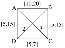
By applying the above definition to all the distinct pairs of edges in $G$ we obtain the sought partial order. To see that the order is only partial in general, consider the example graph in Figure 1. We have defined such a graph $G$ by drawing the graphical structure and specifying set-based weights by placing intervals on the edges in a separate way (i.e., assuming logical independency between different intervals). That is, the example graph is equivalent to the set $\mathcal{G}$ of graphs obtained by choosing real weights within the intervals in all the possible ways. Now observe that the intervals for the edges (A,B) and (B,C) overlap, so that there is no dominance in either direction. Figure 2 shows the overall partial order on the edges for the graph in Figure 1.

Figure 1: An example set-based weighted graph. The sets for the edges are specified separately by intervals that in two cases degenerate to real numbers.

Figure 2: The partial order on the edges of the graph in the preceding figure. Here an arrow from $e$ to $e^{\prime}$ means that $e$ dominates $e^{\prime}$.

Now we consider the set $\mathcal{O}$ of all the total orders that extend the partial order induced by Definition 1. Of course, $\mathcal{O}$ includes $\mathcal{O_{T}}$. They coincide if for each total order in $\mathcal{O}$, there is a graph $G_{w}\in\mathcal{G}$ in which $w(e)>w(e^{\prime})$ if $e$ dominates $e^{\prime}$ in the given total order. This is the case, for example, when mutual information is separately specified via intervals on the edges.

3.1 Exact detection of strong edges

We call strong edges the edges of $G$ that are common to all the trees in $\mathcal{T}$. Identifying the strong edges allows us to robustly infer dependencies that belong to the unknown optimal approximating trees. The following theorem is the central tool for the identification.

Theorem 2.

Assume $\mathcal{O}=\mathcal{O_{T}}$. An edge $e$ of $G$ is strong if and only if in each simple cycle that contains $e$ there is an edge $e^{\prime}$ dominated by $e$.

Proof.

∎

($\Leftarrow$) By contradiction, assume that there is a graph $G_{w}\in\mathcal{G}$ for which an optimal tree $T$ does not contain $e$. By adding $e$ to $T$ we create a cycle [PS82, Proposition 2]. By hypothesis, in such a cycle there must exist an edge $e^{\prime}$ dominated by $e$, so $w(e)>w(e^{\prime})$. Removing $e^{\prime}$, we obtain a new tree that improves upon $T$, so that $T$ cannot be optimal for $G_{w}$.

($\Rightarrow$) By contradiction, assume that there is a cycle $C$ in $G$ where $e$ does not dominate any edge. Then there is a total order in $\mathcal{O}$ in which $e$ is dominated by any other edge $e^{\prime}$ in $C$. Since $\mathcal{O}=\mathcal{O_{T}}$, there must also exist a related graph $G_{w}$ for which $w(e)\leq w(e^{\prime})$ for any edge $e^{\prime}$ in $C$. Call $T$ the related tree. By removing $e$ from $T$ we create two subtrees, say $T^{\prime}$ and $T^{\prime\prime}$. One of these can possibly be a degenerate tree composed by a single node. Now consider that there must be an edge $e_{C}$ of $C$ that connects a node of $T^{\prime}$ with one of $T^{\prime\prime}$. If there was not, there would be no way to start from an endpoint of $e$ in $T^{\prime}$ and reach the other endpoint, because all the paths would be confined within $T^{\prime}$. The graph composed by $T^{\prime}$, $T^{\prime\prime}$ and $e_{C}$ has $m-1$ edges, spans all the nodes of $G$, and therefore it is a tree, say $T^{*}$ [PS82, Proposition 2]. If $w(e)<w(e_{C})$, $T^{*}$ improves upon $T$, so that $T$ cannot be optimal for $G_{w}$. If $w(e)=w(e_{C})$, both $T^{*}$ and $T$ are optimal, but their intersection does not contain $e$, so $e\notin\mathcal{T}$.

Theorem 2 directly leads to a procedure that determines whether or not a given edge $e$ is strong. It suffices to consider the graph $G^{\prime}$ obtained from $G$ by removing $e$ and the edges that $e$ dominates (see the Procedure ‘DetectStrongEdges’ in Table 3). Edge $e$ is strong if and only if its endpoints are not connected in $G^{\prime}$. By applying this procedure to the graph in Figure 1, we conclude that only (A,B) is strong.

Note that Theorem 2 assumes that $\mathcal{O}$ coincides with $\mathcal{O_{T}}$. If this failed to be true, $\mathcal{O_{T}}\subset\mathcal{O}$ would still hold, making Theorem 2 work with a set of trees larger than $\mathcal{T}$, eventually leading to an excess of caution: the edges determined by the above procedure would anyway be strong, but there might be strong edges that the procedure would not be able to determine.

As for computational considerations, note that testing whether or not two nodes are connected in a graph demands $O(m^{2})$ time. Repeating the test for all the edges $e\in E$, we have the computational complexity of the overall procedure, $O(m^{4})$.

3.2 Approximate detection of strong edges

This section presents a procedure that approximately detects the strong edges, reducing the complexity to $O(m^{3})$ with respect to the exact procedure given in Section 3.1.

Consider the algorithm outlined in a pseudo programming language in Table 1. It takes as input a fully connected graph $G=<V,E>$. In the algorithm, a tree with a number of nodes in $\{2,\ldots,m-1\}$ is called subtree.

2. Let $SE=\emptyset$;

3. for each $v\in V$

   1. if there is a node $v^{\prime}\in V$ such that $(v,v^{\prime})\notin SE$ and it dominates $(v,v^{\prime\prime})$ for each $v^{\prime\prime}\in V$, $v^{\prime\prime}\neq v^{\prime}$ then

      1. add $(v,v^{\prime})$ to $SE$;

4. if there is a subtree in $SE$ then

   1. make it the current subtree;

   2. consider the set of edges $E^{\prime}\subseteq E$ with one endpoint in the nodes of the current subtree and the other outside;

   3. if there is an edge $e^{\prime}\in E^{\prime}$ that dominates all the other edges in $E^{\prime}$ then

      1. add $e^{\prime}$ to $SE$ and to the current subtree;

      2. go to 3b;

   4. else

      1. if there is another subtree in $SE$ not considered yet then

         1. go to 3a;

      2. else output $SE$.

Table 1: Approximate procedure to detect strong edges.

The following proposition shows that the algorithm in Table 1 returns only strong edges.

Proposition 3.

$SE$ is a subset of the strong edges of $G$.

Proof.

Consider the first possible insertion in Step 2(a)i. The cycles that encompass $(v,v^{\prime})$ must pass through the set of edges $\{(v,v^{\prime\prime}):v^{\prime\prime}\in V,v^{\prime\prime}\neq v^{\prime}\}$. Since $(v,v^{\prime})$ dominates all the edges in the preceding set, for each cycle passing through $(v,v^{\prime})$ there is an edge in the cycle that is dominated by $(v,v^{\prime})$, so that $(v,v^{\prime})$ is strong, by Theorem 2.

The algorithm can insert an edge in $SE$ also in Step 3(c)i. Recall that each subtree is a connected acyclic graph. It is clear that any cycle that contains $e^{\prime}$ must pass through an edge $e^{\prime\prime}$ that has one endpoint in the nodes of the subtree and the other outside. But $e^{\prime}$ dominates $e^{\prime\prime}$ by Step 3c. This holds for all the cycles, so $e^{\prime}$ is strong by Theorem 2. ∎

The logic of the algorithm in Table 1 is to move from subtrees made of strong edges to adjacent nodes, in order to detect the strong edges of a graph. This policy does not allow all the strong edges to be determined in general. For example, the approximate algorithm cannot determine that the edge (A,B) in Figure 1 is strong.

The heuristic policy implements a trade-off between computational complexity and the capability to fully detect the strong edges. This choice does not seem critical to the specific extent of discovering tree-dependency structures. In fact, the knowledge of the actual mutual information increases with the sample size, becoming a number in the limit. It is easy to check that in these conditions the exact and the approximate procedure produce the same set of edges.

Computational complexity

The assumption behind the following analysis is that the comparison of two edges can be done in constant time. In this case, given a set $E^{\prime}$ of edges, there is a procedure that determines in time $O(\left|E^{\prime}\right|)$ if there is an edge $e^{\prime}\in E^{\prime}$ that dominates all the others. The first step of the procedure selects an edge that is candidate to be dominant. This is made by doing pairwise comparisons of edges and by always discarding the non-dominant edge (or edges) in the comparison. After at most $\left|E^{\prime}\right|-1$ comparisons, we know whether there is a candidate or not. If there is, the second step of the procedure compares such candidate $e^{\prime}$ with all the other edges, deciding if $e^{\prime}$ dominates all the others. This requires $\left|E^{\prime}\right|-1$ comparisons. The two steps of the procedure take $O(\left|E^{\prime}\right|$) time.

Let us now focus on the algorithm in Table 1. The loop 2 is repeated $m=\left|V\right|$ times. Each time the test 2a decides whether there is a dominant edge out of $m-1$ edges (each node is connected to all the others). By the previous result, such task takes $O(m)$ time. Then the loop requires $O(m^{2})$ time.

Now consider the two nested loops made by the instructions 3a, 3b, 3(c)ii, and 3iA. Each time the instruction of jump 3(c)ii is executed, a new edge has been added to $SE$. Each time 3iA is executed, a new subtree is considered. Since $SE$ can have $m-1$ edges at most and $m$ is also an upper bound on the number of different subtrees, the two loops can jointly require $2m-1$ iterations at most. Each such iteration executes the test 3c. By using $m^{2}$ as an upper bound on $\left|E^{\prime}\right|$, we need $O(m^{2})$ time to detect whether the dominant edge exists. The overall time required by the loops is $O(m^{3})$. This is also the computational complexity of the entire procedure.

4 Robust comparison of edges

So far we have focused on the detection of strong edges, taking for granted that there exists a method to partially compare edges based on imprecise knowledge of mutual information. We provide such a method in the following sections. We will first present a formal introduction to the imprecise Dirichlet model in Section 4.1. Section 4.2 will make a first step by computing robust estimates for the entropy. These will be used in Section 4.3 to derive robust estimates of mutual information. Finally, the method to compare edges will be given in Section 4.4.

4.1 The imprecise Dirichlet model

Random i.i.d. processes

We consider a discrete random variable $\imath$ and a related i.i.d. random process with samples $i\in\{1,...,d\}$ drawn with probability $\pi_{i}$. The chances ${\boldsymbol{\pi}}$ form a probability distribution, i.e., ${\boldsymbol{\pi}}\in\Delta:=\{\boldsymbol{x}\in I\negthinspace\negthinspace R^{d}\thinspace:\thinspace x_{i}\geq 0\thinspace\forall i,\thickspace x_{\scriptscriptstyle+}=1\}$, where we have used the abbreviation $x_{\scriptscriptstyle+}:=\sum_{i=1}^{d}x_{i}$. The likelihood of a specific data set $\boldsymbol{D}=(i_{1},...,i_{n})$ with $n_{i}$ samples $i$ and total sample size $n=n_{\scriptscriptstyle+}=\sum_{i}n_{i}$ is $p(\boldsymbol{D}|{\boldsymbol{\pi}})\propto\prod_{i}\pi_{i}^{n_{i}}$. Quantities of interest are, for instance, the entropy ${\cal H}({\boldsymbol{\pi}})=-\sum_{i}\pi_{i}\log\pi_{i}$, where $\log$ denotes the natural logarithm. The chances $\pi_{i}$ are usually unknown and have to be estimated from the data.

Second order p(oste)rior

In the Bayesian approach one models the initial uncertainty in ${\boldsymbol{\pi}}$ by a (second order) prior distribution $p({\boldsymbol{\pi}})$ with domain ${\boldsymbol{\pi}}\in\Delta$. The Dirichlet priors $p({\boldsymbol{\pi}})\propto\prod_{i}\pi_{i}^{n^{\prime}_{i}-1}$, where $n^{\prime}_{i}$ comprises prior information, represent a large class of priors. $n^{\prime}_{i}$ may be interpreted as (possibly fractional) “virtual” sample numbers. High prior belief in $i$ can be modelled by large $n^{\prime}_{i}$. It is convenient to write $n^{\prime}_{i}=s\cdot t_{i}$ with $s:=n^{\prime}_{+}$, hence ${\boldsymbol{t}}\in\Delta$. Examples for $s$ are $0$ for Haldane’s prior [Hal48], $1$ for Perks’ prior [Per47], ${d\over 2}$ for Jeffreys’ prior [Jef46], and $d$ for Bayes-Laplace’s uniform prior [GCSR95] (all with $t_{i}={1\over d}$). These are also called noninformative priors. From the prior and the data likelihood one can determine the posterior $p({\boldsymbol{\pi}}|\boldsymbol{D})=p({\boldsymbol{\pi}}|\boldsymbol{n})\propto\prod_{i}\pi_{i}^{n_{i}+st_{i}-1}$. The expected value or mean $u_{i}:=E_{\boldsymbol{t}}[\pi_{i}]={n_{i}+st_{i}\over n+s}$ is often used for estimating $\pi_{i}$ (the accuracy may be obtained from the covariance of ${\boldsymbol{\pi}}$). The expected entropy is $E_{\boldsymbol{t}}[{\cal H}]=\int_{\Delta}{\cal H}({\boldsymbol{\pi}})p({\boldsymbol{\pi}}|\boldsymbol{n})d{\boldsymbol{\pi}}$. An approximate solution can be obtained by exchanging $E$ with ${\cal H}$ (exact only for linear functions): $E_{\boldsymbol{t}}[{\cal H}({\boldsymbol{\pi}})]\approx{\cal H}(E_{\boldsymbol{t}}[{\boldsymbol{\pi}}])={\cal H}({\boldsymbol{u}})$. The approximation error is typically of the order ${1\over n}$. In [WW95, Hut01, HZ05] exact expressions have been obtained:

$$E_{\boldsymbol{t}}[{\cal H}] = H({\boldsymbol{u}})\thickspace:=\thickspace\sum_{i}h(u_{i}){\quad\mbox{with}\quad}$$ (1)

$$h(u) = u\negthinspace\cdot\negthinspace[\psi(n+s+1)-\psi((n+s)u+1)],$$

where $\psi(x)=d\thinspace\log\Gamma(x)/dx$ is the logarithmic derivative of the Gamma function. There are fast implementations of $\psi$ and its derivatives and exact expressions for integer and half-integer arguments (see Appendix A).

Definition of the imprecise Dirichlet model

There are several problems with noninformative priors. First, the inference generally depends on the arbitrary definition of the sample space. Second, they assume exact prior knowledge $p({\boldsymbol{\pi}})$. The solution to the second problem is to model our ignorance by considering sets of priors $p({\boldsymbol{\pi}})$, a model that is part of the wider theory of imprecise probabilities [Wal91]. The specific imprecise Dirichlet model [Wal96] considers the set of all ${\boldsymbol{t}}\in\Delta$, i.e., $\{p({\boldsymbol{\pi}}):{\boldsymbol{t}}\in\Delta\}$, which solves also the first problem. Walley suggests to fix the hyperparameter $s$ somewhere in the interval $[1,2]$. A set of priors results in a set of posteriors, set of expected values, etc. For real-valued quantities like the expected entropy $E_{\boldsymbol{t}}[{\cal H}]$ the sets are typically intervals:

$$E_{\boldsymbol{t}}[{\cal H}]\thickspace\in\thickspace[\min_{{\boldsymbol{t}}\in\Delta}E_{\boldsymbol{t}}[{\cal H}]\thinspace,\thinspace\max_{{\boldsymbol{t}}\in\Delta}E_{\boldsymbol{t}}[{\cal H}]]\thickspace=:\thickspace[\underline{H},\overline{H}].$$

In the next section we derive approximations for

$$\overline{H}\thickspace=\thickspace\max_{{\boldsymbol{t}}\in\Delta}H({\boldsymbol{u}}){\quad\mbox{and}\quad}\underline{H}\thickspace=\thickspace\min_{{\boldsymbol{t}}\in\Delta}H({\boldsymbol{u}}).$$

One can show that $h(u)$ is strictly concave (see Appendix A), i.e.,  $h^{\prime\prime}(u)<0$ and that $h^{\prime\prime}$ is monotone increasing ($h^{\prime\prime\prime}>0$), which we exploit in the following. The results for the entropy serve as building blocks to derive similar results for the needed mutual information. We define the general correspondence

$$u_{i}^{\cdots}={n_{i}+st_{i}^{\cdots}\over n+s},\quad\mbox{where ${}^{\ldots}$ can be various superscripts}.$$

4.2 Robust entropy estimates

Taylor expansion of $H({\boldsymbol{u}})$

In the following we derive reliable approximations for $\overline{H}$ and $\underline{H}$. If $n$ is not too small these approximations are close to the exact values. More precisely, the length of interval $[\underline{H},\overline{H}]$ is $O(\sigma)$, where $\sigma:={s\over n+s}$, while the approximations will differ from $\overline{H}$ and $\underline{H}$ by at most $O(\sigma^{2})$. Let $t_{i}^{*}\in[0,1]$ and $u_{i}^{*}={n_{i}+st_{i}^{*}\over n+s}$. This implies

$$u_{i}-u_{i}^{*}\thickspace=\thickspace\sigma\negthinspace\cdot\negthinspace(t_{i}-t_{i}^{*}){\quad\mbox{and}\quad}|u_{i}-u_{i}^{*}|\thickspace=\thickspace\sigma|t_{i}-t_{i}^{*}|\thickspace\leq\thickspace\sigma.$$ (2)

Hence we may Taylor-expand $H({\boldsymbol{u}})$ around ${\boldsymbol{u}}^{*}$. $H$ is approximately linear in ${\boldsymbol{u}}$ and hence in ${\boldsymbol{t}}$. A linear function on a simplex assumes its extreme values at the vertices of the simplex. The most natural point for expansion is $t_{i}^{*}={1\over d}$ in the center of $\Delta$. For this choice the bound (2) and most of the following bounds can be improved to $\sigma\leadsto\sigma|1-{1\over d}|$. Other, even data-dependent choices like $t_{i}^{*}={n_{i}\over n}=u_{i}^{*}$, are possible. The only property we use in the following is that $\arg\max_{i}u_{i}^{*}=\arg\max_{i}n_{i}$ and $\arg\min_{i}u_{i}^{*}=\arg\min_{i}n_{i}$. We have

$$H({\boldsymbol{u}})\thickspace=\thickspace\overbrace{H({\boldsymbol{u}}^{*})}^{H_{0}=O(1)}+\overbrace{\sum_{i}h^{\prime}(u_{i}^{*})(u_{i}-u_{i}^{*})}^{H_{1}=O(\sigma)}+\overbrace{{\textstyle{1\over 2}}\sum_{i}h^{\prime\prime}(\check{u}_{i})(u_{i}-u_{i}^{*})^{2}}^{H_{R}=O(\sigma^{2})}.$$

For suitable $\check{u}_{i}$ between $u_{i}^{*}$ and $u_{i}$ this expansion is exact ($H_{R}$ is the exact remainder).

Approximation of $\overline{H}$

Inserting (2) into $H_{1}$ we get

$$H_{1}\thickspace=\thickspace\sum_{i}h^{\prime}(u_{i}^{*})(u_{i}-u_{i}^{*})\thickspace=\thickspace\sigma\sum_{i}h^{\prime}(u_{i}^{*})(t_{i}-t_{i}^{*}).$$

Ignoring the $O(\sigma^{2})$ remainder $H_{R}$, in order to maximize $H({\boldsymbol{u}})$ we only have to maximize $\sum_{i}h^{\prime}(u_{i}^{*})t_{i}$ (the only ${\boldsymbol{t}}$-dependent part). A linear function on $\Delta$ is maximized by setting the $t_{i}$ component with largest coefficient to 1. Due to concavity of $h$, $h^{\prime}(u_{i}^{*})$ is largest for the smallest $u_{i}^{*}$, i.e.,  for smallest $n_{i}$, i.e.,  for $i=\overline{i}:=\arg\min_{i}n_{i}$. Hence $\overline{H_{1}}=H_{1}(\overline{\boldsymbol{u}})$, where $\overline{t}_{i}:=\delta_{i,\overline{i}}$ and $\overline{\boldsymbol{u}}$ follows from $\overline{\boldsymbol{t}}$ by the general correspondence. $H_{0}+\overline{H_{1}}$ is an $O(\sigma^{2})$ approximation of $\overline{H}$. Consider now the remainder $H_{R}$:

$$H_{R}\thickspace=\thickspace{\textstyle{1\over 2}}\sigma^{2}\sum_{i}h^{\prime\prime}(\check{u}_{i})|t_{i}-t_{i}^{*}|^{2}\thickspace\leq\thickspace 0\thickspace=:\thickspace H_{R}^{ub}$$

due to $h^{\prime\prime}<0$. This bound cannot be improved in general, since $H_{R}=0$ is attained for $t_{i}=t_{i}^{*}$. Non-positivity of $H_{R}$ shows that $H_{0}+\overline{H_{1}}$ is an upper bound of $\overline{H}$. Since $\overline{H}\geq H({\boldsymbol{u}})$ for all ${\boldsymbol{u}}$, $H(\overline{\boldsymbol{u}})$ in particular is a lower bound on $\overline{H}$, and moreover also an $O(\sigma^{2})$ approximation. Together we have

$$\underbrace{H(\overline{\boldsymbol{u}})}_{\overline{H}-O(\sigma^{2})}\thickspace\leq\thickspace\overline{H}\thickspace\leq\thickspace\underbrace{H_{0}+\overline{H_{1}}}_{\overline{H}+O(\sigma^{2})}.$$

For robust estimates, the upper bound is, of course, more interesting.

Approximation of $\underline{H}$

The determination of $\underline{H_{1}}$ follows the same scheme as for $\overline{H_{1}}$. We get $\underline{H_{1}}=H_{1}(\underline{{\boldsymbol{u}}})$ with $\underline{t}_{i}:=\delta_{i,\underline{i}}$ and $\underline{i}:=\arg\max_{i}n_{i}$. Using $|t_{i}-t_{i}^{*}|\leq 1$, $\check{u}_{i}\geq{n_{i}\over n+s}$, $h^{\prime\prime}<0$ and that $h^{\prime\prime}$ is monotone increasing ($h^{\prime\prime\prime}>0$) we get the following lower bound on the remainder $H_{R}$:

$$H_{R}\thickspace=\thickspace{\textstyle{1\over 2}}\sigma^{2}\sum_{i}h^{\prime\prime}(\check{u}_{i})|t_{i}-t_{i}^{*}|^{2}\thickspace\geq\thickspace{\textstyle{1\over 2}}\sigma^{2}\sum_{i}h^{\prime\prime}(\textstyle{n_{i}\over n+s})\thickspace=:\thickspace H_{R}^{lb}.$$

Putting everything together we have

$$\underbrace{H_{0}+\underline{H_{1}}}_{\underline{H}-O(\sigma^{2})}+\underbrace{H_{R}^{lb}}_{O(\sigma^{2})}\thickspace\leq\thickspace\underline{H}\thickspace\leq\thickspace\underbrace{H(\underline{{\boldsymbol{u}}})}_{\underline{H}+O(\sigma^{2})}.$$

For robust estimates, the lower bound is more interesting. General approximation techniques for other quantities of interest are developed in [Hut03]. Exact expressions for $[\underline{H},\overline{H}]$ are also derived there.

4.3 Robust estimates for mutual information

Mutual information

Here we generalize the bounds for the entropy found in Section 4.2 to the mutual information of two random variables $\imath$ and $\jmath$ that take values in $\{1,...,d_{\imath}\}$ and $\{1,...,d_{\jmath}\}$, respectively. Consider an i.i.d. random process with samples $(i,j)\in\{1,...,d_{\imath}\}\times\{1,...,d_{\jmath}\}$ drawn with joint probability $\pi_{ij}$, where ${\boldsymbol{\pi}}\in\Delta:=\{\boldsymbol{x}\in I\negthinspace\negthinspace R^{d_{\imath}\times d_{\jmath}}\thinspace:\thinspace x_{ij}\geq 0\thinspace\forall ij,\thickspace x_{\scriptscriptstyle++}=1\}$. We are interested in the mutual information of $\imath$ and $\jmath$:

$${\cal I}({{\boldsymbol{\pi}}}) = \sum_{i=1}^{d_{\imath}}\sum_{j=1}^{d_{\jmath}}\pi_{ij}\log{\pi_{ij}\over\pi_{i{\scriptscriptstyle+}}\pi_{{\scriptscriptstyle+}j}}$$

$$= \sum_{ij}\pi_{ij}\log\pi_{ij}-\sum_{i}\pi_{i{\scriptscriptstyle+}}\log\pi_{i{\scriptscriptstyle+}}-\sum_{j}\pi_{{\scriptscriptstyle+}j}\log\pi_{{\scriptscriptstyle+}j}$$

$$= {\cal H}({\boldsymbol{\pi}}_{\imath{\scriptscriptstyle+}})+{\cal H}({\boldsymbol{\pi}}_{{\scriptscriptstyle+}\jmath})-{\cal H}({\boldsymbol{\pi}}_{\imath\jmath}).$$

$\pi_{i{\scriptscriptstyle+}}=\sum_{j}\pi_{ij}$ and $\pi_{{\scriptscriptstyle+}j}=\sum_{i}\pi_{ij}$ are marginal probabilities. Again, we assume a Dirichlet prior over ${\boldsymbol{\pi}}_{\imath\jmath}$, which leads to a Dirichlet posterior $p({\boldsymbol{\pi}}_{\imath\jmath}|\boldsymbol{n})\propto\prod_{ij}\pi_{ij}^{n_{ij}+st_{ij}-1}$. The expected value of $\pi_{ij}$ is

$$u_{ij}:=E_{\boldsymbol{t}}[\pi_{ij}]={n_{ij}+st_{ij}\over n+s}.$$

The marginals ${\boldsymbol{\pi}}_{i{\scriptscriptstyle+}}$ and ${\boldsymbol{\pi}}_{{\scriptscriptstyle+}j}$ are also Dirichlet with expectation $u_{i{\scriptscriptstyle+}}$ and $u_{{\scriptscriptstyle+}j}$. The expected mutual information $E_{\boldsymbol{t}}[{\cal I}]$ can, hence, be expressed in terms of the expectations of three entropies

$$I({\boldsymbol{u}}):=H({\boldsymbol{u}}_{\imath{\scriptscriptstyle+}})+H({\boldsymbol{u}}_{{\scriptscriptstyle+}\jmath})-H({\boldsymbol{u}}_{\imath\jmath})\thickspace=\thickspace H_{left}+H_{right}-H_{joint}$$

$$\thickspace=\thickspace\sum_{i}h(u_{i{\scriptscriptstyle+}})+\sum_{j}h(u_{{\scriptscriptstyle+}j})-\sum_{ij}h(u_{ij})$$

where here and in the following we index quantities with joint, left, and right to denote to which distribution the quantity refers. Using (1) we get $E_{\boldsymbol{t}}[{\cal I}]=I({\boldsymbol{u}})$.

Crude bounds for $I({\boldsymbol{u}})$

Estimates for the IDM interval $[\min_{{\boldsymbol{t}}\in\Delta}E_{\boldsymbol{t}}[{\cal I}]$, $\max_{{\boldsymbol{t}}\in\Delta}E_{\boldsymbol{t}}[{\cal I}]]$ can be obtained by minimizing/maximizing $I({\boldsymbol{u}})$. A crude upper bound can be obtained as

$$\overline{I}\thickspace:=\thickspace\max_{{\boldsymbol{t}}\in\Delta}I({\boldsymbol{u}})\thickspace=\thickspace\max[H_{left}+H_{right}-H_{joint}]\thickspace\leq\thickspace$$

$$\max H_{left}+\max H_{right}-\min H_{joint}\thickspace=\thickspace\overline{H}_{left}+\overline{H}_{right}-\underline{H}_{joint},$$

where upper and lower bounds to $\overline{H}_{left}$, $\overline{H}_{right}$ and $\underline{H}_{joint}$ have been derived in Section 4.2. Similarly $\underline{I}\geq\underline{H}_{left}+\underline{H}_{right}-\overline{H}_{joint}$. The problem with these bounds is that, although good in some cases, they can become arbitrarily crude. In the following we derive bounds similar to the entropy case with $O(\sigma^{2})$ accuracy.

$O(\sigma^{2})$ bounds for $I({\boldsymbol{u}})$

We expand $I({\boldsymbol{u}})$ around ${\boldsymbol{u}}^{*}$ with a constant term $I_{0}$, a term $I_{1}$ linear in $\sigma$ and an exact $O(\sigma^{2})$ remainder.

$$I({\boldsymbol{u}})\thickspace=\thickspace I_{0}+I_{1}+I_{R},\qquad I_{0}=H_{0left}+H_{0right}-H_{0joint}=I({\boldsymbol{u}}^{*}),$$

$$I_{1} =\thickspace H_{1left}+H_{1right}-H_{1joint}$$

$$= \sum_{i}h^{\prime}(u_{i{\scriptscriptstyle+}}^{*})(u_{i{\scriptscriptstyle+}}\negthinspace\negthinspace-\negthinspace u_{i{\scriptscriptstyle+}}^{*})+\sum_{j}h^{\prime}(u_{{\scriptscriptstyle+}j}^{*})(u_{{\scriptscriptstyle+}j}\negthinspace-\negthinspace u_{{\scriptscriptstyle+}j}^{*})-\sum_{ij}h^{\prime}(u_{ij}^{*})(u_{ij}\negthinspace-\negthinspace u_{ij}^{*})$$

$$= \sigma\sum_{ij}g_{ij}(t_{ij}-t_{ij}^{*}){\quad\mbox{with}\quad}g_{ij}:=h^{\prime}(u_{i{\scriptscriptstyle+}}^{*})+h^{\prime}(u_{{\scriptscriptstyle+}j}^{*})-h^{\prime}(u_{ij}^{*}).$$

$I_{1}$ is maximal if $\sum_{ij}g_{ij}t_{ij}$ is maximal. This is maximal if $t_{ij}=\overline{t}_{ij}:=\delta_{(ij),\overline{(ij)}}$ and $\overline{(ij)}:=\arg\max_{(ij)}g_{ij}$, hence $\overline{I_{1}}=I_{1}(\overline{\boldsymbol{u}})$, and $I_{0}+\overline{I_{1}}$ and $I(\overline{\boldsymbol{u}})$ being $O(\sigma^{2})$ approximations to $\overline{I}$. Replacing all max’s by min’s we get $I_{0}+\underline{I_{1}}$ and $I(\underline{{\boldsymbol{u}}})$ as $O(\sigma^{2})$ approximations to $\underline{I}$. To get robust bounds we need bounds on $I_{R}=H_{R\thinspace left}+H_{R\thinspace right}-H_{R\thinspace joint}.$

$$I_{R} \leq \max_{{\boldsymbol{u}},\boldsymbol{\check{u}}}[H_{R\thinspace left}+H_{R\thinspace right}-H_{R\thinspace joint}]$$

$$\leq H_{R\thinspace left}^{ub}+H_{R\thinspace right}^{ub}-H_{R\thinspace joint}^{lb}\thickspace=\thickspace-H_{R\thinspace joint}^{lb}=:I_{R}^{ub}.$$

$$I_{R} \geq \min_{{\boldsymbol{u}},\boldsymbol{\check{u}}}[H_{R\thinspace left}\negthinspace+\negthinspace H_{R\thinspace right}\negthinspace-\negthinspace H_{R\thinspace joint}]$$

$$\geq H_{R\thinspace left}^{lb}\negthinspace+\negthinspace H_{R\thinspace right}^{lb}\negthinspace-\negthinspace H_{R\thinspace joint}^{ub}=H_{R\thinspace left}^{lb}\negthinspace+\negthinspace H_{R\thinspace right}^{lb}=:I_{R}^{lb}.$$

Note that for $H_{R}$ we can tolerate such a crude approximation, since $H_{R}$ (and $H_{R}^{ub/lb}$) are small $O(\sigma^{2})$ corrections. In summary we have

$$\overbrace{I(\overline{\boldsymbol{u}})}^{\overline{I}-O(\sigma^{2})} \leq \overline{I}\thickspace\leq\thickspace\overbrace{I_{0}+\overline{I_{1}}}^{\overline{I}+O(\sigma^{2})}+\overbrace{I_{R}^{ub}}^{O(\sigma^{2})}{\quad\mbox{and}\quad}$$

$$\underbrace{I_{0}+\underline{I_{1}}}_{\underline{I}-O(\sigma^{2})}+\underbrace{I_{R}^{lb}}_{O(\sigma^{2})} \leq \underline{I}\thickspace\leq\thickspace\underbrace{I(\underline{{\boldsymbol{u}}})}_{\underline{I}+O(\sigma^{2})}.$$

4.4 Comparing edges

For two edges $a$ and $b$ with no common vertex, the reliable interval containing $[\underline{I},\overline{I}]$ of Section 4.3 can be used separately for $a$ and $b$. For edges with a common vertex the results of Section 4.3 may still be used, but they may no longer be reliable or good from a global perspective. Consider the subgraph $\imath\stackrel{{\scriptstyle a}}{{\mbox{---}}}\jmath\stackrel{{\scriptstyle b}}{{\mbox{---}}}\kappa$, joint probabilities $\pi_{\imath\jmath\kappa}$ of vertices $\imath$, $\jmath$, $\kappa$, a Dirichlet posterior $\prod_{ij{\dot{\kappa}}}\pi_{ij{\dot{\kappa}}}^{n_{ij{\dot{\kappa}}}+st_{ij{\dot{\kappa}}}-1}$, $u_{ij{\dot{\kappa}}}=E_{\boldsymbol{t}}[\pi_{ij{\dot{\kappa}}}]={n_{ij{\dot{\kappa}}}+st_{ij{\dot{\kappa}}}\over n+s}$, etc. The expected mutual information between node $\imath$ and $\jmath$ is $I^{a}:=I({\boldsymbol{u}}^{a})$ and $I^{b}:=I({\boldsymbol{u}}^{b})$ between $\jmath$ and $\kappa$, where $u^{a}_{ij}=u_{ij{\scriptscriptstyle+}}$ and $u^{b}_{j{\dot{\kappa}}}=u_{{\scriptscriptstyle+}j{\dot{\kappa}}}$. The weight of edge $a$ is $w^{a}=[\min\thinspace I^{a},\max\thinspace I^{a}]$, where $\min$ and $\max$ are w.r.t. $t^{a}_{ij}:=t_{ij{\scriptscriptstyle+}}$. Similarly, the weight of edge $b$ is $w^{b}=[\min\thinspace I^{b},\max\thinspace I^{b}]$, where $\min$ and $\max$ is w.r.t. $t^{b}_{j{\dot{\kappa}}}:=t_{{\scriptscriptstyle+}j{\dot{\kappa}}}$. The results of Section 4.3 can be used to determine the intervals. Unfortunately this procedure neglects the constraint $t^{a}_{{\scriptscriptstyle+}j}=t^{b}_{j{\scriptscriptstyle+}}$. The correct treatment is to define $w^{a}$ larger than $w^{b}$ as follows:

$$[w^{a}>w^{b}]\quad\Leftrightarrow\quad[I^{a}>I^{b}\thickspace\mbox{for all}\thickspace t_{\imath\jmath\kappa}\in\Delta]\quad\Leftrightarrow\quad\min_{\boldsymbol{t}}[I^{a}-I^{b}]>0.$$

The crude approximation $\min[I^{a}-I^{b}]\geq\min I^{a}-\max I^{b}$ gives back the above naive interval comparison procedure. This shows that the naive procedure is reliable, but the approximation may be crude. For good estimates we proceed similar as in Section 4.3 to get $O(\sigma^{2})$ approximations and bounds on $I^{a}-I^{b}$.

$$\overbrace{I^{a}_{0}\negthinspace-\negthinspace I^{b}_{0}\negthinspace+\negthinspace I^{a}_{1}(\underline{{\boldsymbol{u}}})\negthinspace-\negthinspace I^{b}_{1}(\underline{{\boldsymbol{u}}})}^{\min[I^{a}-I^{b}]-O(\sigma^{2})}+\overbrace{I^{a.lb}_{R}-I^{b.ub}_{R}}^{O(\sigma^{2})}\leq\min_{{\boldsymbol{t}}\in\Delta}[I^{a}\negthinspace-\negthinspace I^{b}]\leq\overbrace{I^{a}(\underline{{\boldsymbol{u}}})\negthinspace-\negthinspace I^{b}(\underline{{\boldsymbol{u}}})}^{\min[I^{a}-I^{b}]+O(\sigma^{2})}$$

$$\underline{(ij{\dot{\kappa}})}:=\mathop{\rm arg\thinspace min}_{ij{\dot{\kappa}}}[h^{\prime}(u_{i{\scriptscriptstyle++}}^{*})-h^{\prime}(u_{ij{\scriptscriptstyle+}}^{*})-h^{\prime}(u_{{\scriptscriptstyle++}{\dot{\kappa}}}^{*})+h^{\prime}(u_{{\scriptscriptstyle+}j{\dot{\kappa}}}^{*})]$$

$$=\arg\limits_{(ij{\dot{\kappa}})}\{\min_{j}[\min_{i}(h^{\prime}(u_{i{\scriptscriptstyle++}}^{*})-h^{\prime}(u_{ij{\scriptscriptstyle+}}^{*}))+\min_{\dot{\kappa}}(h^{\prime}(u_{{\scriptscriptstyle+}j{\dot{\kappa}}}^{*})-h^{\prime}(u_{{\scriptscriptstyle++}{\dot{\kappa}}}^{*}))]\}$$

and $\underline{t}_{ij{\dot{\kappa}}}:=\delta_{(ij{\dot{\kappa}}),\underline{(ij{\dot{\kappa}})}}$, and, for instance, choosing $t_{ij{\dot{\kappa}}}^{*}={1\over d_{\imath}d_{\jmath}d_{\kappa}}$ or $t_{ij{\dot{\kappa}}}^{*}={n_{ij{\dot{\kappa}}}\over n}=u_{ij{\dot{\kappa}}}^{*}$. The second representation for $\underline{(ij{\dot{\kappa}})}$ shows that $\underline{(ij{\dot{\kappa}})}$, and hence the bounds, can be computed in time $O(d^{2})$ rather than $O(d^{3})$. Note that $\min_{i}$ and $\min_{\dot{\kappa}}$ determine $i$ and ${\dot{\kappa}}$ as a function of $j$, then $\min_{j}$ determines $\underline{j}$, which can be used to get $\underline{i}=i(\underline{j})$ and $\underline{{\dot{\kappa}}}={\dot{\kappa}}(\underline{j})$. This lower bound on $\min[I^{a}-I^{b}]$ is used in the next section to robustly compare weights.

5 An example

This section illustrates the application of the developed methodology to an artificial problem.

Figure 3: A graph that models the dependencies between the random variables of an artificial domain.

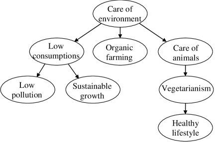
The graph in Figure 3 models the domain by relationships of direct dependency, represented by directed arcs. Each node represents a binary (yes-no) variable that is associated with the probability distribution of the variable itself conditional on the state of the parent node. The distributions are given in Table 2.

Variable	P(variable=yes$|$parent=yes)	P(variable=yes$|$parent=no)
Care of environment	0.366	0.366
Low consumptions	0.959	0.460
Organic farming	0.950	0.450
Care of animals	0.801	0.332
Low pollution	1.000	0.208
Sustainable growth	0.951	0.200
Vegetarianism	0.993	0.460
Healthy lifestyle	0.920	0.300

Table 2: Conditional probability distributions for the variables of the example in Figure 3. (The distribution of ‘Care of environment’ is represented in this table though it is actually unconditional.)

A model made by the graph and the probability tables, as the one above, is called a Bayesian network [Pea88]. We used the Bayesian network to sample units from the joint distribution of the variables in the graph. Each unit is a vector that represents a joint instance of all the variables. By the generated data set we can test our algorithm for the discovery of strong edges, and compare it with Chow and Liu’s algorithm.

The ‘strong edges algorithm’ is summarized for clarity in Table 3. The main procedure is called ‘DetectStrongEdges’ and it implements the exact procedure from Section 3.1. The comparison of edges needed by ‘DetectStrongEdges’ is implemented by the subprocedure ‘TestDominance’. The test 2(a)vii there exploits the bounds defined in Section 4.3 (we have added superscripts $a$ and $b$ to the terms of the bounds to make it clear to which edge they refer). For edges with a common node, the test 2(b)vi exploits the bounds given in Section 4.4. For the dominance tests we have used the value 1 for the IDM hyper-parameter $s$ (see Section 4.1). We have also chosen $t_{ij}^{*}=\frac{1}{d_{\imath}d_{\jmath}}$, $t_{ij{\dot{\kappa}}}^{*}=\frac{1}{d_{\imath}d_{\jmath}d_{\kappa}}$, etc.

1. Procedure DetectStrongEdges(a set-based weighted graph $G$)

   1. forest:=$\emptyset$;

   2. for each edge $e\in E$

      1. consider $G^{\prime}$ obtained from $G$ dropping $e$ and the edges it dominates;

      2. if the endpoints of $e$ are not connected in $G^{\prime}$, add $e$ to forest;

   3. return forest.

2. Procedure TestDominance(edge $a$, edge $b$)

   1. if $a$ and $b$ do not share nodes then (i.e., the edges are $\imath\stackrel{{\scriptstyle a}}{{\mbox{---}}}\jmath$ and $\tilde{\imath}\stackrel{{\scriptstyle b}}{{\mbox{---}}}\tilde{\jmath}$)

      1. $I^{a}_{0}:=\sum_{i}h(u_{i+}^{*})+\sum_{j}h(u_{+j}^{*})-\sum_{ij}h(u_{ij}^{*})$;

      2. $I^{b}_{0}:=\sum_{\tilde{i}}h(u_{\tilde{i}+}^{*})+\sum_{\tilde{j}}h(u_{+\tilde{j}}^{*})-\sum_{\tilde{i}\tilde{j}}h(u_{\tilde{i}\tilde{j}}^{*})$;

      3. $\underline{I_{1}^{a}}:=\thickspace\thickspace\thickspace\sigma\thinspace\min_{ij}[h^{\prime}(u_{i+}^{*})+h^{\prime}(u_{+j}^{*})-h^{\prime}(u_{ij}^{*})]$
                 $-\sigma\sum_{ij}t_{ij}^{*}[h^{\prime}(u_{i+}^{*})+h^{\prime}(u_{+j}^{*})-h^{\prime}(u_{ij}^{*})]$;

      4. $\overline{I_{1}^{b}}:=\thickspace\thickspace\thickspace\sigma\thinspace\max_{\tilde{i}\tilde{j}}[h^{\prime}(u_{\tilde{i}+}^{*})+h^{\prime}(u_{+\tilde{j}}^{*})-h^{\prime}(u_{\tilde{i}\tilde{j}}^{*})]$
                 $-\sigma\sum_{\tilde{i}\tilde{j}}t_{\tilde{i}\tilde{j}}^{*}[h^{\prime}(u_{\tilde{i}+}^{*})+h^{\prime}(u_{+\tilde{j}}^{*})-h^{\prime}(u_{\tilde{i}\tilde{j}}^{*})]$;

      5. $I^{a.lb}_{R}:=\frac{1}{2}\sigma^{2}\sum_{i}h^{\prime\prime}(\frac{n_{i+}}{n+s})+\frac{1}{2}\sigma^{2}\sum_{j}h^{\prime\prime}(\frac{n_{+j}}{n+s})$;

      6. $I^{b.ub}_{R}:=-\frac{1}{2}\sigma^{2}\sum_{\tilde{i}\tilde{j}}h^{\prime\prime}(\frac{n_{\tilde{i}\tilde{j}}}{n+s})$;

      7. if $I_{0}^{a}-I_{0}^{b}+\underline{I_{1}^{a}}-\overline{I_{1}^{b}}+I_{R}^{a.lb}-I_{R}^{b.ub}>0$, return ‘true’;

   2. else (i.e., the edges are $\imath\stackrel{{\scriptstyle a}}{{\mbox{---}}}\jmath\stackrel{{\scriptstyle b}}{{\mbox{---}}}\kappa$)

      1. $I^{a}_{0}:=\sum_{i}h(u_{i++}^{*})+\sum_{j}h(u_{+j+}^{*})-\sum_{ij}h(u_{ij+}^{*})$;

      2. $I^{b}_{0}:=\sum_{j}h(u_{+j+}^{*})+\sum_{\dot{\kappa}}h(u_{++{\dot{\kappa}}}^{*})-\sum_{j{\dot{\kappa}}}h(u_{+j{\dot{\kappa}}}^{*})$;

      3. $\underline{I_{1}^{a}-I_{1}^{b}}:=\sigma\thinspace\min_{j}[\min_{i}(h^{\prime}(u_{i{\scriptscriptstyle++}}^{*})-h^{\prime}(u_{ij{\scriptscriptstyle+}}^{*}))+\min_{\dot{\kappa}}(h^{\prime}(u_{{\scriptscriptstyle+}j{\dot{\kappa}}}^{*})-h^{\prime}(u_{{\scriptscriptstyle++}{\dot{\kappa}}}^{*}))]$
         $-\sigma\sum_{j}[d_{\kappa}\sum_{i}t_{ij{\dot{\kappa}}}^{*}(h^{\prime}(u_{i{\scriptscriptstyle++}}^{*})-h^{\prime}(u_{ij{\scriptscriptstyle+}}^{*}))+d_{\imath}\sum_{\dot{\kappa}}t_{ij{\dot{\kappa}}}^{*}(h^{\prime}(u_{{\scriptscriptstyle+}j{\dot{\kappa}}}^{*})-h^{\prime}(u_{{\scriptscriptstyle++}{\dot{\kappa}}}^{*}))]$;

      4. $I^{a.lb}_{R}:=\frac{1}{2}\sigma^{2}\sum_{i}h^{\prime\prime}(\frac{n_{i++}}{n+s})+\frac{1}{2}\sigma^{2}\sum_{j}h^{\prime\prime}(\frac{n_{+j+}}{n+s})$;

      5. $I^{b.ub}_{R}:=-\frac{1}{2}\sigma^{2}\sum_{j{\dot{\kappa}}}h^{\prime\prime}(\frac{n_{+j{\dot{\kappa}}}}{n+s})$;

      6. if $I^{a}_{0}-I^{b}_{0}+\underline{I_{1}^{a}-I_{1}^{b}}+I^{a.lb}_{R}-I^{b.ub}_{R}>0$, return ‘true’;

   3. return ‘false’.

3. Procedure h($u$) return $u\psi(n+s+1)-u\psi(nu+su+1)$;

4. Procedure h^′($u$) return $\psi(n+s+1)-\psi(nu+su+1)-u(n+s)\psi^{\prime}(nu+su+1)$;

5. Procedure h^′′($u$) return $-2(n+s)\psi^{\prime}(nu+su+1)-u(n+s)^{2}\psi^{\prime\prime}(nu+su+1)$;

Table 3: A summary view of the strong edges algorithm. Remember that $\sigma=\frac{s}{n+s}$, $n$ is the sample size, $u_{\cdots}=\frac{n_{\cdots}+t_{\cdots}}{n+s}$ denotes the expectation of a certain chance, $u_{\cdots}^{*}$ the expectation taken for a specific value $t_{\cdots}^{*}$ of hyper-parameter $t_{\cdots}$; finally, $\psi$ denotes the $\psi$-function, described in Appendix A.

a.   Strong edges algorithm b.   Chow and Liu’s algorithm

Figure 4: The outputs of the two algorithms after reading 20 instances.

a.   Strong edges algorithm b.   Chow and Liu’s algorithm

Figure 5: The outputs of the two algorithms after reading 30 instances.

a.   Strong edges algorithm b.   Chow and Liu’s algorithm

Figure 6: The outputs of the two algorithms after reading 40 instances.

a.   Strong edges algorithm b.   Chow and Liu’s algorithm

Figure 7: The outputs of the two algorithms after reading 50 instances.

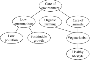
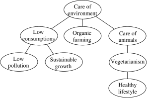
Figures 4 to 7 show the progression of the models discovered by the two algorithms as more instances are read. The strong edges algorithm appears to behave more reliably than Chow and Liu’s algorithm. It suspends the judgment on ambiguous cases and outputs forests. These are always composed of edges of the actual graph. Chow and Liu’s algorithm always produces complete trees, but these misrepresent the actual tree until 50 instances have been read. At this point Chow and Liu’s algorithm detects the right tree. The cautious approach implemented by the strong edges algorithm needs other 20 instances to produce the same complete tree.

6 Extensions

The methodology developed so far leads naturally to other possible extensions of Chow and Liu’s approach. We briefly report on two different types of extensions in the following.

Section 6.1 discusses the question of tree-dependency structures vs. forest-dependency structures under several respects. The discussion focuses both on algorithms that are alternative to the strong edges one, and that aim at yielding trees, and on the other hand on algorithms that emphasize the inference of forest-dependency structures from data.

In Section 6.2 we extend the computation of lower and upper expectations of mutual information to the computation of robust credible limits. These are intervals for mutual information obtained from the IDM that contain the actual value with given probability. This result is useful in order to produce dependency structures that provide the user with a given guarantee level. In principle the extension to credible limits can be applied both to the computation of strong edges and to that of robust trees, as defined in the next section, although the results of Sections 6.1 and 6.2 are actually independent, in the sense that one does not need to use them together.

6.1 Forests vs. Trees

It may be useful to critically re-consider Chow and Liu’s algorithm in the following respect. Chow and Liu’s algorithm yields always a tree by construction, and hence this happens also when the actual (but usually unknown) dependency structure is a forest. This is a questionable characteristic of the algorithm, as in the mentioned case yielding a tree seems to be hard to justify. There are indeed approaches in the literature of precise probability that suppress the edges of a maximum spanning tree for which the mutual information is not large enough, yielding a forest. This is typically implemented using a numerical threshold $\varepsilon$, sometimes computed via statistical tests. Such approaches can be used immediately also within the imprecise-probability framework introduced in this paper; it is sufficient to suppress the edges for which the upper value of mutual information [i.e., $\max_{w\in W}w(e)$] does not exceed $\varepsilon$. In contrast with the precise-probability approach, the latter should have the advantage to better deal with the problem to suppress edges by mistake, as a consequence of the variability of the inferred values of mutual information. This should be especially true once forests are inferred using the credible limits for mutual information introduced in the next section.

A more subtle question is how the forests inferred using the above threshold procedure relate to the forests that are naturally produced by the strong edges algorithm in its original form. Remind that the strong edges algorithm produces a forest rather than a tree when there is more than one optimal tree consistent with the available data; indeed the algorithm aims at yielding the graphical structure made of the intersection of all such trees. The situation may be clarified by focusing on a special case: consider a problem in which the true dependency structure is a tree in which there are edges with the same value of mutual information, say $\mu$. In this case the strong edges algorithm will never produce a tree, only a forest, also in the limit of infinitely many data. The reason is that there will always be multiple optimal trees consistent with the data, just because multiple optimal trees are a characteristic of the problem. In particular, there would arise a forest because some edges with weight $\mu$ would never belong to the set of strong edges. Now suppose that $\mu>\varepsilon$. In this case, the previous threshold procedure would not suppress the edges with mutual information equal to $\mu$. In other words, the two procedures suppress edges under different conditions: the strong edges algorithm may suppress edges because they have equal true values of mutual information, despite those values may be high; the threshold procedure only suppresses edges with low value of mutual information. For this reason it could make sense to apply the threshold procedure also as a post-processing step of the strong edges algorithm.

The discussion so far has highlighted an interesting point. By focusing on the intersection of all the trees consistent with the data, the strong edges algorithm appears to be well suited as a tool to recover the actual dependency structure underlying the data. This is because the algorithm does not aim at recovering just any of the equivalent structures, rather, it focuses on the common pattern to all of them, which is obviously part of the actual structure. In this sense, the strong edges algorithm might be well suited for applications concerned with the recovery of causal patterns.

On the other hand, one can think of applications for which the algorithm is probably not so well suited. For instance, in (precise-probability) problems of pattern classification based on Bayesian networks [FGG97], it is important to recover any tree (or forest) structure for which the sum of the edge weights is maximized. In this case, suppressing edges with large weights only because they are not strong might lead to low classification accuracy. In these cases, the extension of those precise approaches to the IDM-based inferential approach should probably follow other lines than those described here. One possibility could be to exploit existing results in the literature of robust optimization; the work of Yaman et al. [YKP01] seems to be particularly worthy of consideration. Yaman et al. consider a problem of maximum spanning tree for a graph with weights specified by intervals (the weights are given no particular interpretation), which is a special case of a set-based weighted graph. They define the relative robust spanning tree as follows (using our notations): let $T$ be a generic tree spanning $G$, and denote by $T^{*}_{w}$ a maximum spanning tree of $G_{w}\in\mathcal{G}$. Let $S^{*}_{w}$ resp. $S_{w}$ be the sum of the edge weights of $T^{*}_{w}$ resp. $T$, with respect to the weight function $w$. A relative robust spanning tree $T^{*}$ is one that solves the optimization problem $\min_{T}\max_{w\in W}(S_{w}^{\ast}-S_{w})$, i.e., one that minimizes the largest deviation $S_{w}^{\ast}-S_{w}$ among all the possible graphs $G_{w}\in\mathcal{G}$. In this sense the approach adopted by Yaman et al. is in the long tradition of the popular maximin (or minimax) decision criterion. From the computational point of view, although the problem is NP-complete [AVH04], recent results show that relatively large instances of the problem can be solved efficiently [Mon0X]. The trees defined by Yaman et al. could probably be combined with the IDM-based inferential approach presented here, suitably modified for classification problems, in order to yield relative robust classification trees. Here, too, it could make sense to post-process the relative robust trees in order to suppress edges with small upper (or even lower) values of mutual information, yielding a forest.

6.2 Robust credible limits for mutual information

In this section we develop a full inferential approach for mutual information under the IDM.

An $\alpha$-credible interval for the mutual information $\cal I$ is an interval $[{\smash{\mathop{\cal I}\limits_{\widetilde{}}}}{},\widetilde{\cal I}]$ which contains $\cal I$ with probability at least $\alpha$, i.e.,  $\int_{{\smash{\mathop{\cal I}\limits_{\widetilde{}}}}{}}^{\widetilde{\cal I}}p({\cal I})d{\cal I}\geq\alpha$. We define $\alpha$-credible intervals w.r.t. distribution $p_{\boldsymbol{t}}({\cal I})$ as

$$[{\smash{\mathop{\cal I}\limits_{\widetilde{}}}}{}_{\boldsymbol{t}},\widetilde{\cal I}_{\boldsymbol{t}}]\thickspace=\thickspace[E_{\boldsymbol{t}}[{\cal I}]-{\smash{\mathop{\Delta\cal I}\limits_{\widetilde{}}}}{}_{\boldsymbol{t}}\thinspace,\thinspace E_{\boldsymbol{t}}[{\cal I}]+\widetilde{\Delta\cal I}_{\boldsymbol{t}}]{\quad\mbox{such that}\quad}\int_{{\smash{\mathop{\cal I}\limits_{\widetilde{}}}}{}_{\boldsymbol{t}}}^{\widetilde{\cal I}_{\boldsymbol{t}}}p_{\boldsymbol{t}}({\cal I})d{\cal I}\geq\alpha,$$

where $\widetilde{\Delta\cal I}_{\boldsymbol{t}}:=\widetilde{\cal I}_{\boldsymbol{t}}-E_{\boldsymbol{t}}[{\cal I}]$ (${\smash{\mathop{\Delta\cal I}\limits_{\widetilde{}}}}{}_{\boldsymbol{t}}:=E_{\boldsymbol{t}}[{\cal I}]-{\smash{\mathop{\cal I}\limits_{\widetilde{}}}}{}_{\boldsymbol{t}}$) is the distance from the right boundary $\widetilde{\cal I}_{\boldsymbol{t}}$ (left boundary ${\smash{\mathop{\cal I}\limits_{\widetilde{}}}}{}_{\boldsymbol{t}}$) of the $\alpha$-credible interval $[{\smash{\mathop{\cal I}\limits_{\widetilde{}}}}{}_{\boldsymbol{t}},\widetilde{\cal I}_{\boldsymbol{t}}]$ to the mean $E_{\boldsymbol{t}}[{\cal I}]$ of $\cal I$ under distribution $p_{\boldsymbol{t}}$. We can use

$$[{\smash{\mathop{\cal I}\limits_{\simeq}}}{},\overline{\widetilde{\cal I}}]\thickspace:=\thickspace[\min_{\boldsymbol{t}}{\smash{\mathop{\cal I}\limits_{\widetilde{}}}}{}_{\boldsymbol{t}},\max_{\boldsymbol{t}}\widetilde{\cal I}_{\boldsymbol{t}}]\thickspace=\thickspace\bigcup_{\boldsymbol{t}}\thinspace[{\smash{\mathop{\cal I}\limits_{\widetilde{}}}}{}_{\boldsymbol{t}},\widetilde{\cal I}_{\boldsymbol{t}}]$$

as a robust credible interval, since $\int_{{\smash{\mathop{\cal I}\limits_{\simeq}}}{}}^{\overline{\widetilde{\cal I}}}p_{\boldsymbol{t}}({\cal I})d{\cal I}\geq\int_{{\smash{\mathop{\cal I}\limits_{\widetilde{}}}}{}_{\boldsymbol{t}}}^{\widetilde{\cal I}_{\boldsymbol{t}}}p_{\boldsymbol{t}}({\cal I})d{\cal I}\geq\alpha$ for all ${\boldsymbol{t}}$. An upper bound for $\overline{\widetilde{\cal I}}$ (and similarly lower bound for ${\smash{\mathop{\cal I}\limits_{\simeq}}}{}$) is

$$\overline{\widetilde{\cal I}}\thickspace=\thickspace\max_{\boldsymbol{t}}(E_{\boldsymbol{t}}[{\cal I}]+\widetilde{\Delta\cal I}_{\boldsymbol{t}})\thickspace\leq\thickspace\max_{\boldsymbol{t}}E_{\boldsymbol{t}}[{\cal I}]+\max_{\boldsymbol{t}}\widetilde{\Delta\cal I}_{\boldsymbol{t}}\thickspace=\thickspace\overline{E[{\cal I}]}+\overline{\widetilde{\Delta\cal I}}.$$

Good upper bounds on $\overline{I}=\overline{E[{\cal I}]}$ have been derived in Section 4.3.

For not too small $n$, $p_{\boldsymbol{t}}({\cal I})$ is close to Gaussian due to the central limit theorem. So we may approximate $\widetilde{\Delta\cal I}_{\boldsymbol{t}}\approx r\sigma_{\boldsymbol{t}}$ with $r$ given by $\alpha=\mbox{erf}(r/\sqrt{2})$, where erf is the error function (e.g.,  $r=2$ for $\alpha\approx 95\%)$ and $\sigma_{\boldsymbol{t}}$ is the variance of $p_{\boldsymbol{t}}$, keeping in mind that this could be a non-conservative approximation. In order to determine $\overline{\widetilde{\Delta\cal I}}$ we only need to estimate $\max_{\boldsymbol{t}}\sqrt{{\mbox{Var}}_{\boldsymbol{t}}[{\cal I}]}=O({1\over n})$. The variation of $\sqrt{{\mbox{Var}}_{\boldsymbol{t}}[{\cal I}]}$ with ${\boldsymbol{t}}$ is of order $n^{-3/2}$. If we regard this as negligibly small, we may simply fix some ${\boldsymbol{t}}^{*}\in\Delta$. So the robust credible interval for $\cal I$ can be estimated as

$$\overline{\widetilde{\cal I}}\thickspace\leq\thickspace\overline{I}+\overline{\widetilde{\Delta\cal I}}\thickspace\leq\thickspace I_{0}+\overline{I_{1}}+I_{R}^{ub}+\overline{\widetilde{\Delta\cal I}}\thickspace\approx\thickspace I_{0}+\overline{I_{1}}+I_{R}^{ub}+r\sqrt{{\mbox{Var}}_{{\boldsymbol{t}}^{*}}[{\cal I}]}.$$

Expressions for the variance of $\cal I$ have been derived in [Hut01, HZ05]:

$${\mbox{Var}}_{\boldsymbol{t}}[{\cal I}]={1\over n\negthinspace+\negthinspace s}\sum_{ij}u_{ij}\bigg{(}\log{u_{ij}\over u_{i{\scriptscriptstyle+}}u_{{\scriptscriptstyle+}j}}\bigg{)}^{2}\negthinspace-\negthinspace{1\over n+s}\bigg{(}\sum_{ij}u_{ij}\log{u_{ij}\over u_{i{\scriptscriptstyle+}}u_{{\scriptscriptstyle+}j}}\bigg{)}^{2}\negthinspace\negthinspace+O(n^{-2}).$$

Higher order corrections to the variance and higher moments have also been derived, but are irrelevant in light of our other approximations. In Sections 4.4 and 5 we also needed a lower bound on $I^{a}-I^{b}$. Taking credible intervals into account we need a robust upper $\alpha$-credible limit for ${\cal I}^{ba}:={\cal I}^{b}-{\cal I}^{a}$. Similarly as for the variance one can derive the following expression:

$$\overline{\widetilde{{\cal I}^{\smash{ba}}}} \leq I^{b}_{0}-I^{a}_{0}+\overline{I^{b}_{1}}-\underline{I^{a}_{1}}+I^{b.ub}_{R}-I^{a.lb}_{R}+$$

$$r\sqrt{{\mbox{Var}}_{{\boldsymbol{t}}^{*}}[{\cal I}^{b}-{\cal I}^{a}]}+O(n^{-3/2}),$$

$${\mbox{Var}}_{\boldsymbol{t}}[{\cal I}^{b}-{\cal I}^{a}] = {\mbox{Var}}_{\boldsymbol{t}}[{\cal I}^{b}]+{\mbox{Var}}_{\boldsymbol{t}}[{\cal I}^{a}]-2{\mbox{Cov}}_{\boldsymbol{t}}[{\cal I}^{b},{\cal I}^{a}],$$

$${\mbox{Cov}}_{\boldsymbol{t}}[{\cal I}^{b},{\cal I}^{a}] = {1\over n+s}\sum_{ij{\dot{\kappa}}}u_{ij{\dot{\kappa}}}\bigg{(}\log{u^{a}_{ij}\over u^{a}_{i{\scriptscriptstyle+}}u^{a}_{{\scriptscriptstyle+}j}}\log{u^{b}_{j{\dot{\kappa}}}\over u^{b}_{j{\scriptscriptstyle+}}u^{b}_{{\scriptscriptstyle+}{\dot{\kappa}}}}\bigg{)}$$

$$-{1\over n+s}\bigg{(}\sum_{ij}u^{a}_{ij}\log{u^{a}_{ij}\over u^{a}_{i{\scriptscriptstyle+}}u^{a}_{{\scriptscriptstyle+}j}}\bigg{)}\bigg{(}\sum_{j{\dot{\kappa}}}u^{b}_{j{\dot{\kappa}}}\log{u^{b}_{j{\dot{\kappa}}}\over u^{b}_{j{\scriptscriptstyle+}}u^{b}_{{\scriptscriptstyle+}{\dot{\kappa}}}}\bigg{)}\thickspace+\thickspace O(n^{-2}).$$

Variances are typically of order $1/n$, so for large $n$, credible intervals $\overline{\widetilde{\cal I}}-{\smash{\mathop{\cal I}\limits_{\simeq}}}{}=O(1/\sqrt{n})$ are much wider than expected intervals $\overline{I}-\underline{I}=O(1/n)$.

7 Conclusions

This paper has tackled the problem to reliably infer trees from data. We have provided an exact procedure that infers strong edges in time $O(m^{4})$, and have shown that it performs well in practice on an example problem. We have also developed an approximate algorithm that works in time $O(m^{3})$.

Reliability follows from using the IDM, a robust inferential model that rests on very weak prior assumptions. Working with the IDM involves computing lower and upper estimates, i.e., solving global optimization problems. These can hardly be tackled exactly, as they are typically non-linear and non-convex. A substantial part of the present work has been devoted to provide systematic approximations to the exact intervals with a guaranteed worst case of $O(\sigma^{2})$. This was achieved by optimizing approximating functions, obtained by Taylor-expanding the original objective function. We have taken care to make these approximations conservative, i.e., they always include the exact interval. This is the necessary step to ultimately obtain over-cautious rather than overconfident models.

More broadly speaking, the same approach has been used also for another approximation, concerned with the representation level chosen for the IDM. In principle, one might use the IDM for the joint realization of all the $m$ random variables. In this paper we have used one IDM for each bivariate (and tri-variate, in some cases) realization. Using separate IDMs simplifies the treatment, but it may give rise to global inconsistencies (in the same lines of the discussion on comparing edges with a common vertex, in Section 4.4). However, their effect is only to make $\mathcal{O}$ strictly include $\mathcal{O_{T}}$, thus producing an excess of caution, as discussed in Section 3.1.

We have already reported two developments that follow naturally from the work described above. The first involves the computation of robust trees, which widens the scope of this paper to other applications. The second is in the direction of even greater robustness by providing robust credibile limits for mutual information, which provide the user with a guarantee level on the inferred dependency structures.

Other extensions of the present work could be considered that need further research in order to be realized. Obviously, it would be worth extending the work to the robust inference of more general dependency structures. This could be achieved, for example, in a way similar to Kleiter’s work [Kle99]. One could also extend our approach to dependency measures other than mutual information, like the statistical coefficient $\phi^{2}$ [KS67, pp. 556–561]. This would require new approximations to be derived for the new index under the IDM, but the first part of the paper on the detection of strong edges could be applied as it is.

Another important extension could be realized by considering the inference of dependency structures from incomplete samples. Recent research has developed robust approaches to incomplete samples that make very weak assumptions on the mechanism responsible for the missing data [Man02, RS01, Zaf02]. This would be an important step towards realism and reliability in structure inference.

Appendix A Properties of the digamma $\psi$ function

The digamma function $\psi$ is defined as the logarithmic derivative of the Gamma function. Integral representations for $\psi$ and its derivatives are

$$\psi(z) = {d\ln\Gamma(z)\over dz}={\Gamma^{\prime}(z)\over\Gamma(z)}=\int_{0}^{\infty}\left[{e^{-t}\over t}-{e^{-zt}\over 1-e^{-t}}\right]dt,$$

$$\psi^{(\ell)}(z) = (-1)^{\ell+1}\int_{0}^{\infty}{t^{\ell}e^{-zt}\over 1-e^{-t}}dt{\quad\mbox{for}\quad}\ell>0.$$

The $h$ function (1) and its derivatives are $h^{(\ell)}(u)\thickspace=\thickspace$

$$u^{(\ell)}\psi(n\negthinspace+\negthinspace s\negthinspace+\negthinspace 1)-\ell(n\negthinspace+\negthinspace s)^{\ell-1}\psi^{(\ell-1)}((n\negthinspace+\negthinspace s)u\negthinspace+\negthinspace 1)-u(n\negthinspace+\negthinspace s)^{\ell}\psi^{(\ell)}((n\negthinspace+\negthinspace s)u\negthinspace+\negthinspace 1).$$

At argument $u_{i}={n_{i}+st_{i}\over n+s}$ we get for $h$, $h^{\prime}$ and $h^{\prime\prime}$

$$h(u_{i}) = (n_{i}\negthinspace+\negthinspace st_{i})[\psi(n\negthinspace+\negthinspace s\negthinspace+\negthinspace 1)-\psi(n_{i}\negthinspace+\negthinspace st_{i}\negthinspace+\negthinspace 1)]/(n\negthinspace+\negthinspace s),$$

$$h^{\prime}(u_{i}) = \psi(n\negthinspace+\negthinspace s\negthinspace+\negthinspace 1)-\psi(n_{i}\negthinspace+\negthinspace st_{i}\negthinspace+\negthinspace 1)-(n_{i}\negthinspace+\negthinspace st_{i})\psi^{\prime}(n_{i}\negthinspace+\negthinspace st_{i}\negthinspace+\negthinspace 1),$$

$$h^{\prime\prime}(u_{i}) = -2(n\negthinspace+\negthinspace s)\psi^{\prime}(n_{i}\negthinspace+\negthinspace st_{i}\negthinspace+\negthinspace 1)-(n_{i}\negthinspace+\negthinspace st_{i})(n\negthinspace+\negthinspace s)\psi^{\prime\prime}(n_{i}\negthinspace+\negthinspace st_{i}\negthinspace+\negthinspace 1),$$

For integral arguments the following closed representations for $\psi$, $\psi^{\prime}$, and $\psi^{\prime\prime}$ exist:

$$\psi(n\negthinspace+\negthinspace 1)=-\gamma+\sum_{i=1}^{n}{1\over i},\quad\psi^{\prime}(n\negthinspace+\negthinspace 1)={\pi^{2}\over 6}-\sum_{i=1}^{n}{1\over i^{2}},\quad\psi^{\prime\prime}(n\negthinspace+\negthinspace 1)=-2\zeta(3)+2\sum_{i=1}^{n}{1\over i^{3}}$$

where $\gamma=0.5772156...$ is Euler’s constant and $\zeta(3)=1.202569...$ is Riemann’s zeta function at 3. Closed expressions for half-integer values and fast approximations for arbitrary arguments also exist. The following asymptotic expansion can be used if one is interested in $O(({s\over n+s})^{2})$ approximations only (and not rigorous bounds):

$$\psi(z+1)=\log z+{1\over 2z}-{1\over 12z^{2}}+O({1\over z^{4}}).$$

See [AS74] for details on the $\psi$ function and its derivatives. From the above expressions one may show $h^{\prime\prime}<0$ and $h^{\prime\prime\prime}>0$.

References

- [AS74] M. Abramowitz and I. A. Stegun, editors. Handbook of Mathematical Functions. Dover publications, inc., 1974.
- [AVH04] I. D. Aron and P. Van Hentenryck. On the complexity of the robust spanning tree problem with interval data. Operations Research Letters, 32:36–40, 2004.
- [Ber01] J.-M. Bernard. Non-parametric inference about an unknown mean using the imprecise Dirichlet model. In G. de Cooman, T. Fine, and T. Seidenfeld, editors, ISIPTA’01, pages 40–50, The Netherlands, 2001. Shaker Publishing.
- [Ber05] J.-M. Bernard. An introduction to the imprecise Dirichlet model for multinomial data. International Journal of Approximate Reasoning, 39(2–3):123–150, 2005.
- [CL68] C. K. Chow and C. N. Liu. Approximating discrete probability distributions with dependence trees. IEEE Transactions on Information Theory, IT-14(3):462–467, 1968.
- [FGG97] N. Friedman, D. Geiger, and M. Goldszmidt. Bayesian networks classifiers. Machine Learning, 29(2/3):131–163, 1997.
- [GCSR95] A. Gelman, J. B. Carlin, H. S. Stern, and D. B. Rubin. Bayesian Data Analysis. Chapman, 1995.
- [Hal48] J. B. S. Haldane. The precision of observed values of small frequencies. Biometrika, 35:297–300, 1948.
- [Hut01] M. Hutter. Distribution of mutual information. In T. G. Dietterich, S. Becker, and Z. Ghahramani, editors, Proceedings of NIPS*2001, Cambridge, MA, 2001. MIT Press.
- [Hut03] M. Hutter. Robust estimators under the Imprecise Dirichlet Model. In Proc. 3rd International Symposium on Imprecise Probabilities and Their Application (ISIPTA-2003), volume 18 of Proceedings in Informatics, pages 274–289, Canada, 2003. Carleton Scientific.
- [HZ05] M. Hutter and M. Zaffalon. Distribution of mutual information from complete and incomplete data. Computational Statistics & Data Analysis, 48(3):633–657, 2005.
- [Jef46] H. Jeffreys. An invariant form for the prior probability in estimation problems. In Proc. Royal Soc. London (A), volume 186, pages 453–461, 1946.
- [KJ56] J. B. Kruskal Jr. On the shortest spanning subtree of a graph and the traveling salesman problem. In Proc. Am. Math. Soc., volume 7, pages 48–50, 1956.
- [KL51] S. Kullback and R. A. Leiber. On information and sufficiency. Ann. Math. Statistics, 22:79–86, 1951.
- [Kle99] G. D. Kleiter. The posterior probability of Bayes nets with strong dependences. Soft Computing, 3:162–173, 1999.
- [KS67] M. G. Kendall and A. Stuart. The Advanced Theory of Statistics. Griffin, London, 1967. 2nd edition.
- [Kul68] S. Kullback. Information Theory and Statistics. Dover, 1968.
- [Man02] C. Manski. Partial Identification of Probability Distributions. Draft book, Department of Economics, Northwestern University, USA, 2002.
- [Mon0X] R. Montemanni. A Benders decomposition approach for the robust spanning tree problem with interval data. European Journal of Operational Research, 200X. Forthcoming.
- [Pea88] J. Pearl. Probabilistic Reasoning in Intelligent Systems: Networks of Plausible Inference. Morgan Kaufmann, San Mateo, 1988.
- [Per47] W. Perks. Some observations on inverse probability. J. Inst. Actuar., 73:285–312, 1947.
- [PS82] H. Papadimitriou and K. Steiglitz. Combinatorial Optimization: Algorithms and Complexity. Prentice Hall, New York, 1982.
- [RS01] M. Ramoni and P. Sebastiani. Robust learning with missing data. Machine Learning, 45(2):147–170, 2001.
- [VP90] T. Verma and J. Pearl. Equivalence and synthesis of causal models. In P. P. Bonissone, M. Henrion, L. N. Kanal, and J. F. Lemmer, editors, UAI’90, pages 220–227, New York, 1990. Elsevier.
- [Wal91] P. Walley. Statistical Reasoning with Imprecise Probabilities. Chapman and Hall, New York, 1991.
- [Wal96] P. Walley. Inferences from multinomial data: learning about a bag of marbles. J. R. Statist. Soc. B, 58(1):3–57, 1996.
- [WW95] D. H. Wolpert and D. R. Wolf. Estimating functions of distributions from a finite set of samples. Physical Review E, 52(6):6841–6854, 1995.
- [YKP01] H. Yaman, O. E. Karaşan, and M. Ç. Pinar. The robust spanning tree problem with interval data. Operations Research Letters, 29:31–40, 2001.
- [Zaf02] M. Zaffalon. Exact credal treatment of missing data. Journal of Statistical Planning and Inference, 105(1):105–122, 2002.