Network Inference from TraceRoute Measurements: Internet Topology ‘Species’

Abstract

Internet mapping projects generally consist in sampling the network from a limited set of sources by using traceroute probes. This methodology, akin to the merging of spanning trees from the different sources to a set of destinations, leads necessarily to a partial, incomplete map of the Internet. Accordingly, determination of Internet topology characteristics from such sampled maps is in part a problem of statistical inference. Our contribution begins with the observation that the inference of many of the most basic topological quantities – including network size and degree characteristics – from traceroute measurements is in fact a version of the so-called ‘species problem’ in statistics. This observation has important implications, since species problems are often quite challenging. We focus here on the most fundamental example of a traceroute internet species: the number of nodes in a network. Specifically, we characterize the difficulty of estimating this quantity through a set of analytical arguments, we use statistical subsampling principles to derive two proposed estimators, and we illustrate the performance of these estimators on networks with various topological characteristics.

¹LIAFA, CNRS and Université de Paris-7, and LIP6, CNRS and Université de Paris-6, France
² LPT and UMR 8627 du CNRS, Université de Paris-Sud, France
³ Department of Statistics, Rutgers University, USA
⁴ Department of Mathematics and Statistics, Boston University, USA

Keywords: Internet sampling, species problem, statistical inference.

1 Introduction

A significant research and technical challenge in the study of large information networks is related to the incomplete character of the corresponding maps, usually obtained through some sampling process. A prototypical example of this situation is faced in the case of the physical Internet. The topology of the Internet can be investigated at different granularity levels such as the router and Autonomous System (AS) level, with the final aim of obtaining an abstract representation where the set of routers (ASs) and their physical connections (peering relations) are the vertices and edges of a graph, respectively [1, 2]. In the absence of accurate maps, researchers rely on a general strategy that consists in acquiring local views of the network from several vantage points and merging these views. Such local views are obtained by evaluating a certain number of paths to different destinations, through the use of probes or the analysis of routing tables, which we will refer to generically in this paper as ‘traceroute-like sampling’, after the quintissential example of the well-known traceroute tool. The merging of several of these views provides a map of a sampling of the Internet.

While the knowledge of basic Internet topology (i.e., nodes and links) discovered through such sampling is of significant value in and of itself, it is natural to also want to use the resulting sample maps to infer properties of the overall Internet map. With such a strategy in mind, a number of research groups have generated sample maps of the Internet [3, 4, 5, 6, 7] that have then been used for the characterization of network properties. For example, the ‘small world’ character of the Internet has thus been uncovered. Moreover, the probability that any vertex in the graph has degree $k$ (i.e., that it has exactly $k$ links joining it to immediate neighbors) has been characterized as being skewed and heavy-tailed, with an approximately power-law functional form [8].

Recently, the question of the accuracy of the topological characteristics inferred from such maps has been the subject of various studies [9, 10, 11, 12, 13, 14]. Overall, these studies suggest that at a qualitative level the main conclusions drawn from traceroute-like samplings are reliable. For example, it has been found that such samplings allow for accurate discrimination between topologies with degree distributions that are heavy-tailed from those that are homogeneous [12]. On the other hand, at a quantitative level the evidence suggests the possibility for considerable deviations between numerical summaries of characteristics of the sampled networks and those of the actual Internet.

The point of departure for our contributions is the observation that the inference, from traceroute-like measurements, of many common measures of network graph characteristics is in fact related to the so-called ‘species problem’ in statistics. This association with the species problem has important implications because, while the species problem is well-studied, it is also known to be a statistical inference problem that is often particularly difficult. Therefore, for example, in the context of Internet mapping and inference with traceroute, while it is clear that the observed number of nodes, links, and vertex degrees necessarily will underestimate the actual Internet values, it turns out that the accurate adjustment of the observed values may be nontrivial. Furthermore, the unique nature of traceroute-like sampling procedures means that standard tools for species estimation are unlikely to be immediately applicable.

This paper is organized as follows. We provide general background on traceroute and the species problem in Section 2. We then focus on what is arguably the most fundamental species problem in the context of traceroute-like measurements: inferring the number of nodes in a network. In Section 3, we present an analytical argument characterizing the structural elements relevant to this estimation problem. In Section 4, we propose two estimators, derived from principles of statistical subsampling. In Section 5, we describe the results of an extensive numerical evaluation of these estimators. Finally, Section 6 contains some additional discussions and directions for future work.

2 Background

Throughout this paper we will represent an arbitrary network of interest as an undirected, connected graph $\mathcal{G}=(\mathcal{V},\mathcal{E})$, where $\mathcal{V}$ is a set of vertices (nodes) and $\mathcal{E}$ is a set of edges (links). Denote by $N=|\mathcal{V}|$ and $M=|\mathcal{E}|$ the numbers of vertices and edges, respectively. In a typical traceroute study, a set $S=\{s_{1},\ldots,s_{n_{S}}\}$ of $n_{S}$ active sources deployed in the network sends probes to a set $T=\{t_{1},\ldots,t_{n_{T}}\}$ of $n_{T}$ destinations (or targets), for $S,T\subset\mathcal{V}$. Each probe collects information on all the vertices and edges traversed along the path connecting a source to a destination [15]. The actual paths followed by the probes depend on many different factors, such as commercial agreements, traffic congestion, and administrative routing policies, but to a first approximation are often thought of (and frequently modeled as) ‘shortest’ paths. The merging of the various sampled paths yields a partial map of the network (Fig.1). This map may in turn be represented as a sampled subgraph $\mathcal{G}^{*}=(\mathcal{V}^{*},\mathcal{E}^{*})$.

Numerous metrics are used in networking (and indeed across the network-oriented sciences more generally) to summarize characteristics of a network graph $\mathcal{G}$. Some of the most fundamental metrics include the number of vertices, $N$, the number of edges, $M$, and the degrees $\{k_{i}\}$ of vertices $i\in\mathcal{V}$. Many other metrics either may be expressed as explicit functions of these or have closely related behavior. For an arbitrary metric, say $\eta\equiv\eta(\mathcal{G})$, summarizing some characteristic of $\mathcal{G}$, and a traceroute-sampled graph $\mathcal{G}^{*}$, it is natural to wish to produce an estimate, say $\hat{\eta}$ from the measurements underlying $\mathcal{G}^{*}$. However, some caution is in order, in that for the quantities $N$, $M$, and $k_{i}$, the problem of their inference is closely related to the so-called species problem in statistics.

Stated generically, the species problem refers to the situation in which, having observed $n$ members of a (finite or infinite) population, each of whom falls into one of $C$ distinct classes (or ‘species’), an estimate $\hat{C}$ of $C$ is desired. This problem arises in numerous contexts, such as numismatics (e.g., how many of an ancient coin were minted [16]), linguistics (e.g., what was the size of an author’s apparent vocabulary [17, 18]), and biology (e.g., how many species of animals inhabit a given region).

The species problem has received a good deal of attention in statistics. See [19] for an overview and an extensive bibliography. Perhaps surprisingly, however, while the estimation of the relative frequencies of species in a population is well-understood (given knowledge of $C$), the estimation of $C$ itself is often difficult. In essence, what is needed is to estimate the number of species not observed. This task is problematic due to the fact that it is precisely the species present in relatively low proportions in the population that are expected to be missed, and there could be an arbitrarily large number of such species in arbitrarily low proportions. Despite (or perhaps because of) the difficulty of the problem, numerous methods have been proposed for its solution, differing mainly in the assumptions regarding the nature of the population, the type of sampling involved, and the statistical machinery used.

An understanding of the implications of the species problem on network topology inference is of critical importance. For example, we note that in traceroute-like sampling the problem of estimating the number of vertices $N$ in a network graph $\mathcal{G}$ may be mapped to a species problem by considering each separate vertex $i$ as a ‘species’ and declaring a ‘member’ of the species $i$ to have been observed each time that $i$ is encountered on one of the $n=n_{S}\,n_{T}$ traceroute paths. A similar argument shows that estimation of the number of edges $M$ too may be mapped to a species problem. Finally, as in [20], the problem of inferring the degree $k_{i}$ of a vertex $i$ from traceroute measurements can also be mapped to the species problem, by letting all edges incident to $i$ constitute a species and declaring a member of that species to have been observed every time one of those edges is encountered. Because the values $N$, $M$, and $\{k_{i}\}_{i\in\mathcal{V}}$ are both important in their own right and bear important relations to other metrics of interest, it is logical to focus upon the question of their inference. In this paper, we concentrate on the inference of the first of these quantities, $N$.

3 Inferring $N$: Characterization of the Problem

Before proceeding to the construction of estimators for $N$, as we will do in Section 4, it is useful to first better understand the structural elements of the problem. In particular, the following analysis provides insight into the structure of the underlying ‘population’, the relative frequency of the various ‘species’, and the impact of these factors on the problem of inferring $N$. For the sake of exposition, in this section we adopt the common convention of modeling Internet routing, to a first approximation, as ‘shortest-path’ routing. However, we hasten to note that such an assumption, or even an assumption of a static routing protocol, are nowhere made in the derivation of the estimators in Section 4.

A crucial quantity in the characterization of traceroute-like sampling is the so-called betweenness centrality, which essentially counts for each vertex the number of shortest paths on which it lies: nodes with large betweenness lie on many shortest paths and are thus more easily and more frequently probed [12]. More precisely, if ${\cal D}_{hj}$ is the total number of shortest paths from vertex $h$ to vertex $j$, and ${\cal D}_{hj}(i)$ is the number of these shortest paths that pass through the vertex $i$, the betweenness of the vertex $i$ is defined as $b_{i}=\sum{\cal D}_{hj}(i)/{\cal D}_{hj}$, where the sum runs over all $h,j$ pairs with $j\neq h\neq i$. It can be shown [21] that the average shortest path length between pairs of vertices, $\ell$, is related to the betweenness centralities through the expression

$$\sum_{i}b_{i}=N(N-1)(\ell-1)\ .$$

This may be rewritten in the form

$$N=1+\frac{E[b]}{\ell-1}\ ,$$ (1)

where the expectation $E[\cdot]$ is with respect to the distribution of betweenness across nodes in the network i.e., $P(b)=\#\{i\in\mathcal{V}\,:\,b_{i}=b\}/N$.

Empirical experiments suggest that the average shortest path length $\ell$ can be estimated quite accurately, which is not surprising given the path-based nature of traceroute. Therefore, the problem of estimating $N$ is essentially equivalent to that of estimating the average betweenness centrality. Motivated by the fact that Internet maps have been found to display a broad distribution of not only degrees, but also betweenness [12], let us consider a model that pictures the distribution of the betweenness as divided into two parts. That is, we model the distribution $P(b)$ as a mixture distribution [22]

$$P(b)=\pi P_{1}(b)+(1-\pi)P_{2}(b),$$ (2)

where $P_{1}$ is a distribution at low values $b\in[1,b_{min})$, for some $b_{min}$ small, and $P_{2}(b)$ is a distribution at high values $b\in[b_{min},b_{max}]$, $b_{max}>>b_{min}$.

The average $E[{b}]$ in (1) is a weighted combination of two terms i.e., $E[{b}]=\pi E_{1}[b]+(1-\pi)E_{2}[b]$. From the perspective of the simple parametric model just described, the challenge of accurately estimating $E[b]$ – and hence $N$ – can be viewed as a problem of the accurate estimation of the two means, $E_{1}[b]$ and $E_{2}[b]$, and the weight $\pi$. Unfortunately, the first mean, $E_{1}[b]$, requires knowledge of the betweenness of vertices with “small” betweenness. That is, knowledge of nodes $i\in\mathcal{V}$ traversed by relatively few paths. But these are precisely the nodes on which we receive the least information from traceroute-like studies, as they are expected to be visited infrequently or not at all. And the relative proportion $\pi$ of such nodes would seem to be similarly difficult to determine. As mentioned earlier, this is a hallmark characteristic of the species problem, i.e. the lack of accurate knowledge of the relative number in the population of comparitively infrequently observed species.

As for the second mean, $E_{2}$, let us approximate the observed broad distribution of betweeness in the tail by a heavy-tailed power-law form i.e., $P_{2}(b)=b^{-\beta}/K$, where $K$ is a normalization constant. Then

$$E_{2}[{b}]=\frac{1}{K}\int_{{b}_{min}}^{{b}_{max}}{b}^{1-\beta}d{b}\ .$$ (3)

A simple calculation yields $K=({b}_{max}^{1-\beta}-{b}_{min}^{1-\beta})/(1-\beta)$. Additionally, if the only origin of the cutoff is the finite size of the network, ${b}_{max}$ can be defined by imposing the condition that the expected number of nodes beyond the cut-off is bounded by a fixed constant [1]. Therefore one finds that

$$N\times\int_{{b}_{max}}^{\infty}P({b})d{b}\sim 1\quad\Rightarrow\quad{b}_{max}\sim\left(\frac{(\beta-1)K}{(1-\pi)N}\right)^{\frac{1}{1-\beta}}\sim{b}_{min}((1-\pi)N)^{-\frac{1}{1-\beta}},$$ (4)

i.e. a relation between ${b}_{max}$, ${b}_{min}$ $N$, $\pi$ and $\beta$, in which we have also used the assumption ${b}_{min}\ll{b}_{max}$ that implies $K\sim{b}_{min}^{1-\beta}/(\beta-1)$.

Our empirical studies indicate that the exponent $\beta$ can be estimated fairly accurately from the distribution of betweenness’ observed through traceroute measurements. And the above calculations suggest that knowledge of $\beta$ is key to knowledge of $K$. However, note from (4) that $b_{max}$ involves not only the unknown $N$, as would be expected, but also $\pi$, which suggests that even the inference of the $E_{2}$ component of $E[b]$ is potentially impacted by our ability (or lack thereof) to recover information on nodes with low betweenness. Furthermore, we mention that our numerical studies show that $\beta$ is in fact likely quite close to $2$ in the real Internet, which suggests an additional level of subtlety in the accurate estimation of $E_{2}$, due to the nature of the integral in (3).

The above analysis both highlights the relevant aspects of the species problem inherent in estimating $N$ and indicates the futility of attempting a classical parametric estimation approach. One is led, therefore, to consider nonparametric methods, in which models with a small, fixed number of parameters are eschewed in favor of models that essentially have as many parameters as data.

From the perspective of classical nonparametric species models in statistics, the estimation of the total number of vertices $N$, the total number of edges $M$, and the node degree $k_{i}$ are all non-standard statistical inference problems. Consider the classical idealized model where the observed frequencies for different species are truncated Poisson variables conditionally on their positivity. Suppose the Poisson intensities for all the species (including unobserved ones) form a random sample from a completely unknown distribution. Then it is known that in this nonparametric Poisson mixture model, the estimation of the total intensity of unobserved species is a well-posed problem [23, 24], but the estimation of the total number of species is ill-posed [20] from an information theoretical point of view. This indicates the ill-posedness of the problems of estimating $M$ and $k_{i}$ without assuming a parametric model for the distribution of the betweenness centrality, since under Poissonized sampling, the betweenness centrality is proportional to the marginal intensity for links, or species in these problems. However, for the estimation of $N$, vertices are treated as species, and they can be thought of as being first sampled with roughly equal probability as targets and then with unequal probability as intermediate nodes in traceroute experiments. This suggests the estimation of $N$ is more akin to that of the total intensity of unobserved species, since the total unobserved intensity is simply the product of the number of unobserved species and the common intensity when the species are equally likely to be included in the sample. This observation is crucial in our derivation of the leave-one-out estimator in Section 4.2.

4 Estimators of Network Size

A naive estimator of $N$ is simply $N^{*}$, the number of nodes observed in the traceroute study. Given the levels of coverage afforded by the scale of current Internet mapping initiatives, $N^{*}$ can be expected to vastly underestimate $N$ (e.g., [12]). Motivated by the results and discussion in Section 3, in this section we develop two nonparametric estimators for $N$, using subsampling principles.

4.1 A Resampling Estimator

A popular method of subsampling is that of resampling, which underlies the well-known ‘bootstrap’ method [25]. Given a sample $x_{1},...,x_{n}$ from a population, resampling in its simplest form means taking a second sample $x^{*}_{1},...,x^{*}_{m}$ from $x_{1},...,x_{n}$ to study a certain relationship between the first sample and the population through the observed relationship between the second and first samples. We utilize a similar principle here to obtain a factor by which the observed number of vertices $N^{*}$ is inflated to yield an estimator $\hat{N}_{RS}$ of $N$.

Consider the quantity $N^{*}/N$ i.e., the fraction of nodes discovered through traceroute sampling of $\mathcal{G}$, which we will call the discovery ratio. The expected discovery ratio $E[N^{*}/N]$ has been found to vary smoothly as a function of the fraction $q_{T}=n_{T}/N$ of targets sampled, for a given number $n_{S}$ of sources [12, 14]. We will use this fact, paired with an assumption of a type of scaling relation on $\mathcal{G}$, to construct our estimator for $N$. Specifically, we will assume that the sampled subgraph $\mathcal{G}^{*}$ is sufficiently representative of $\mathcal{G}$ so that a sampling ratio on $\mathcal{G}^{*}$ similar to that used in its obtention from $\mathcal{G}$ yields a discovery ratio similar to the fraction of nodes discovered in $\mathcal{G}$.

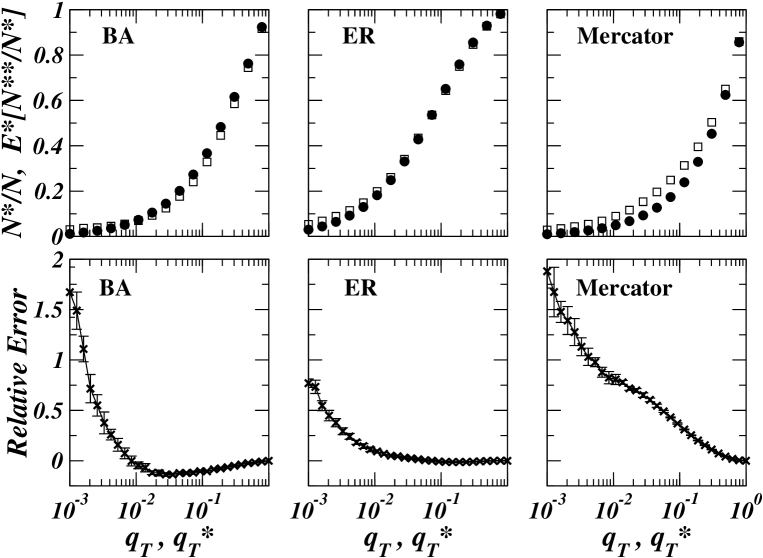
Figure 2: A comparison of the quantities $N^{*}/N$ and $E^{*}[N^{**}]/N^{*}=E[N^{**}|G^{*}]/N^{*}$, as a function respectively of $q_{T}=n_{T}/N$ and $q^{*}_{T}=n^{*}_{T}/N^{*}$, for the three networks described in Section 5. Here $q^{*}_{T}=q_{T}$ and $n_{S}=n_{S}^{*}=10$. Top row shows the averages of $N^{*}/N$ and $E^{*}[N^{**}]/N^{*}$ over 100 realizations of $G^{*}$. Bottom row shows the average of the difference of these two quantities, relative to $N^{*}/N$, over the same 10 realizations. The comparison in the top row confirms the validity of the scaling assumption underlying the resampling estimator derived in Section 4.1, while the comparison in the bottom row indicates better performance of the estimator can be expected with increasing $q_{T}$. (Note: One standard deviation error bars are smaller than the symbol size in most cases.)

That is, suppose that we choose a set $S^{*}$ of $n^{*}_{S}$ source vertices in $\mathcal{G}^{*}$ and a set $T^{*}$ of $n^{*}_{T}$ target vertices, in a manner similar to the way that the original sets $S$ and $T$ underlying $\mathcal{G}^{*}$ were chosen, and such that $q^{*}_{S}\sim q_{S}$ and $q^{*}_{T}\sim q_{T}$, where $q^{*}_{S}=n^{*}_{S}/N^{*}$, $q^{*}_{T}=n^{*}_{T}/N^{*}$, $q_{S}=n_{S}/N$ and $q_{T}$ is defined above. Then we assume that the result of a traceroute study on $\mathcal{G}^{*}$, from sources in $S^{*}$ to targets in $T^{*}$, will yield a subsubgraph, say $\mathcal{G}^{**}$, of $N^{**}$ nodes, such that on average the discovery ratio $N^{**}/N^{*}$ on $\mathcal{G}^{*}$ is similar to the fraction of vertices of $\mathcal{G}$ discovered originally through $\mathcal{G}^{*}$. In other words, we assume that $N^{*}/N\sim E[N^{**}/N^{*}\,|\,\mathcal{G}^{*}]$, where the expectation $E[\,\cdot\,|\mathcal{G}^{*}]$ is with respect to whatever random mechanism drives the choice of source and target sets $S^{*}$ and $T^{*}$ on $\mathcal{G}^{*}$, conditional on fixed $\mathcal{G}^{*}$. Our empirical studies, using uniform random sampling on the networks described in Section 5, suggest that this assumption is quite reasonable over a broad range of values for $q_{T}$, as shown in Fig. 2.

Writing $E^{*}[\cdot]\equiv E[\,\cdot\,|\mathcal{G}^{*}]$, the condition of equal discovery rates can be rewritten in the form $N\sim N^{*}(N^{*}/E^{*}[N^{**}])$. The quantity $E^{*}[N^{**}]$ can be estimated by repeating the resampling experiment just described some number $B$ of times, compiling subsubgraphs $\mathcal{G}^{**}_{1},\ldots,\mathcal{G}^{**}_{B}$ of sizes $N^{**}_{1},\ldots,N^{**}_{B}$, and forming the average $\bar{N}^{**}=(1/B)\sum_{k}N^{**}_{k}$. Substitution then yields

$$\hat{N}_{RS}=N^{*}\,\cdot\,\frac{N^{*}}{\bar{N}^{**}}$$ (5)

as a resampling-based estimator for $N$.

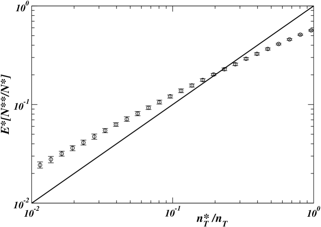
Figure 3: Illustration of the obtention of the resampling estimator, in the case of a BA graph of size $N=10^{5}$. The initial sampling was obtained with $n_{S}=10$ sources and $n_{T}=10^{4}$ targets ($q_{T}=0.1$), yielding a graph $\mathcal{G}^{*}$ of size $N^{*}=33178$ (and $M^{*}=133344$). The circles show the ratio of the average size of the resampled graph $\mathcal{G}^{**}$, $\bar{N}^{**}/N^{*}$, as a function of the ratio $n_{T}^{*}/n_{T}$, with $n_{S}^{*}=n_{S}=10$ sources. The errorbars give the variance with respect to the various placements of sources and targets used for the resampling. The straight line is $y=x$ and allows to find the value of $n_{T}^{*}$ such that $n_{T}/n_{T}^{*}=N^{*}/\bar{N}^{**}$

Note, however, that its derivation is based upon the premise that $q^{*}_{S}=q_{S}$ and $q^{*}_{T}=q_{T}$, and $q_{S},q_{T}$ are unknown (i.e., since $N$ is unknown). To address this issue, we first let $n^{*}_{S}=n_{S}$, since typically the number of sources is too small to make $q_{S}$ a useful quantity. Then we note that the expression $q^{*}_{T}=q_{T}$, in conjunction with our assumption on discovery rates, together imply that $n^{*}_{T}/n_{T}\sim E^{*}[N^{**}]/N^{*}$. With respect to the calculation of $\hat{N}_{RS}$, this fact suggests the strategy of iteratively adjusting $n^{*}_{T}$ until the relation $n^{*}_{T}/n_{T}\approx\bar{N}^{**}/N^{*}$ holds. Alternatively, one may picture the situation geometrically, as shown in Fig. 3. The value of $\bar{N}^{**}$ for the appropriate $n^{*}_{T}$ is then substituted into (5) to produce $\hat{N}_{RS}$. In practice, one may either use a fixed value of $B$ throughout or, as we have done, increase $B$ as the algorithm approaches the condition $n^{*}_{T}/n_{T}\approx\bar{N}^{**}/N^{*}$.

4.2 A ‘Leave-One-Out’ Estimator

Various other subsampling paradigms might be used to construct an estimator. A popular one is the ‘leave-one-out’ strategy underlying such methods as ‘jack-knifing’ [26, 27] and ‘cross-validation’ [25], which amounts to subsampling $\mathcal{G}^{*}$ with $n^{*}_{T}=n_{T}-1$. The same underlying principle may be applied in a useful manner to the problem of estimating $N$, in a way that does not require the scaling assumption underlying (5), as we now describe.

Recall that $\mathcal{V}^{*}$ is the set of all vertices discovered by a traceroute study, including the $n_{S}$ sources $S=\{s_{1},\ldots,s_{n_{S}}\}$ and the $n_{T}$ targets $T=\{t_{1},\ldots,t_{n_{T}}\}$. Our approach will be to connect $N$ to the frequency with which individual targets $t_{j}$ are included in traces from the sources in $S$ to the other targets in $T\setminus\{t_{j}\}$. Accordingly, let $\mathcal{V}^{*}_{i,j}$ be the set of vertices discovered on the path from source $s_{i}$ to target $t_{j}$, inclusive of $s_{i}$ and $t_{j}$. Then the set of vertices discovered as a result of targets other than a given $t_{j}$ can be represented as $\mathcal{V}^{*}_{(-j)}=\cup_{i}\cup_{j^{\prime}\neq j}\mathcal{V}^{*}_{i,j^{\prime}}$. Next define $\delta_{j}=I\left\{t_{j}\notin\mathcal{V}^{*}_{(-j)}\right\}$ to be the indicator of the event that target $t_{j}$ is not ‘discovered’ by traces to any other target. The total number of such targets is $X=\sum_{j}\delta_{j}$.

We will derive a relation between $X$ and $N$ through consideration of the expectation of the former. Under an assumption of simple random sampling in selecting target nodes from $\mathcal{V}$, given a pre-selected (either randomly or not) set of source nodes, we have

$$\Pr\left(\delta_{j}=1\,|\,\mathcal{V}^{*}_{(-j)}\right)=\frac{N-N^{*}_{(-j)}}{N-n_{s}-n_{T}+1}\enskip,$$ (6)

where $N^{*}_{(-j)}=\left|\mathcal{V}^{*}_{(-j)}\right|$. Note that, by symmetry, the expectation $E\left[N^{*}_{(-j)}\right]$ is the same for all $j$: we denote this quantity by $E\left[N^{*}_{(-)}\right]$. As a result of these two facts, we may write

$$E[X]=\sum_{j}\frac{N-E\left[N^{*}_{(-j)}\right]}{N-n_{s}-n_{T}+1}=\frac{n_{T}\left(N-E\left[N^{*}_{(-)}\right]\right)}{N-n_{s}-n_{T}+1}\enskip,$$ (7)

which may be rewritten as

$$N=\frac{n_{T}E\left[N^{*}_{(-)}\right]-(n_{s}+n_{T}-1)E[X]}{n_{T}-E[X]}\enskip.$$ (8)

To obtain an estimator for $N$ from this expression it is necessary to estimate $E\left[N^{*}_{(-)}\right]$ and $E[X]$, for which it is natural to use the unbiased estimators $\bar{N}^{*}_{(-)}=(1/n_{T})\sum_{j}N^{*}_{(-j)}$ and $X$ itself, which is measured during the traceroute study. However, while substitution of these quantities in the numerator of (8) is fine, substitution of $X$ for $E[X]$ in the denominator can be problematic in the event that $X=n_{T}$. Indeed, when none of the targets $t_{j}$ are discovered by traces to other targets, as is possible if $q_{T}=n_{T}/N$ is small, $N$ will be estimated by infinity. A better strategy is to estimate the quantity $1/(n_{T}-X)$ directly. Under the condition that $N^{*}_{(-j)}\approx N^{*}_{(-j^{\prime})}\approx N^{*}_{(-j,-j^{\prime})}$, where $N^{*}_{(-j,-j^{\prime})}=\left|\mathcal{V}^{*}_{(-j)}\cap\mathcal{V}^{*}_{(-j^{\prime})}\right|$, and our assumption of simple random sampling of target vertices, it is possible to produce an approximately unbiased estimator of this quantity, which upon substitution yields

$$\hat{N}_{L1O}=\frac{n_{T}+1}{n_{T}}\,\cdot\,\frac{n_{T}\bar{N}^{*}_{(-)}-(n_{s}+n_{T}-1)X}{n_{T}+1-E[X]}\enskip.$$ (9)

Formal derivation of the leave-one-out estimator $\hat{N}_{L1O}$ in (9) may be found in the appendix. Note that even if $X=n_{T}$, the estimator remains well-defined. The condition that all $\mathcal{V}^{*}_{(-j)}$ and their pairwise intersections have approximately the same cardinality is equivalent to saying that the unique contribution of discovered vertices by any one or any pair of vertices is relatively small. For example, using data collected by the Skitter project at CAIDA [4], a fairly uniform discovery rate of roughly $3$ new nodes per new target, after the initial $200$ targets, has been cited [28]. We have found too that a similar rate held in the empirical experiments of Section 5. Note that this condition also implies that $N^{*}_{(-j)}\approx N^{*}$, for all $j$, which suggests replacement of $\bar{N}^{*}_{(-)}$ by $N^{*}$ in (9). Upon doing so, and after a bit of algebra, we arrive at the approximation

$$\hat{N}_{L1O}\approx(n_{S}+n_{T})\,+\,\frac{N^{*}-(n_{S}+n_{T})}{1-w^{*}}\enskip,$$ (10)

where $w^{*}=X/(n_{T}+1)$, $X$ being the number of targets not discovered by traces to any other target.

In other words, $\hat{N}_{L1O}$ can be seen as counting the $n_{S}+n_{T}$ vertices in $S\cup T$ separately, and then taking the remaining $N^{*}-(n_{S}+n_{T})$ nodes that were ‘discovered’ by traces and adjusting that number upward by a factor of $(1-w^{*})^{-1}$. This form is in fact analogous to that of a classical method in the literature on species problems, due to Good [23], in which the observed number of species is adjusted upwards by a similar factor that attempts to estimate the proportion of the overall population for which no members of species were observed. Such estimators are typically referred to as coverage-based estimators, and a combination of theoretical and numerical evidence seems to suggest that they enjoy somewhat more success than most alternatives [19].

5 Numerical Validation

We examined the performance of the estimators proposed in Section 4 using a methodology similar to those in [12, 10, 14]. That is, we began with known graphs $\mathcal{G}$ with various topological characteristics, equipped each with an assumed routing structure, performed a traceroute-like sampling on them, which yielded a sample graph $\mathcal{G}^{*}$, and computed the estimators $\hat{N}_{RS}$ and $\hat{N}_{L1O}$. This process was repeated a number of times, for various choices of source and target nodes, at each of a range of settings of the parameters $N$, $n_{S}$, and $n_{T}$. A performance comparison was then made by comparing values of $\hat{N}/N$, for $\hat{N}=N^{*},\hat{N}_{RS}$, and $\hat{N}_{L1O}$.

5.1 Design of the Numerical Experiments

Three network topologies were used in our experiments, two synthetic and one based on measurements of the real Internet. The synthetic topologies were generated according to (i) the classical Erdös-Rényi (ER) model [29] and (ii) the network growth model of Albert and Barabási (BA) [30]. This choice of topologies allows us to examine the effects of one of the most basic distinguishing characteristics among networks, the nature of the underlying degree distribution. In particular, the ER model is the standard example of a class of homogeneous graphs, in which the the degree distribution $P(k)$ has small fluctuations and a well defined average degree, while the BA model is the original example of a class of heterogeneous graphs, for which $P(k)$ is a broad distribution with heavy-tail and large fluctuations, spanning various orders of magnitude. In our experiments, we have used randomly generated ER and BA networks with average degree $6$, and sizes $N$ ranging from $10^{3}$ to $10^{6}$ nodes.

The ER and BA models are standard choices for experiments like ours, and useful in allowing one to assess the effect on a proposed methodology of a broad degree distribution, but they lack other important characteristics of the real Internet, such as clustering, complex hierarchies, etc. Therefore, we used as our third topology the Internet sample from MERCATOR [31], a graph with $N=228,263$ nodes and $M=320,149$ edges. While there are newer Internet graphs, such as those from CAIDA [4], our choice of MERCATOR is influenced by the fact that it resulted from an attempt to have obtained an exhaustive map of the Internet in 1999. The aim in presenting such results is primarily illustrative.

Given a graph $\mathcal{G}$, and a chosen set of values for $N$, $n_{S}$, and $n_{T}$, a traceroute-like study was simulated as follows. First, a set of $n_{S}$ sources $S=\{s_{1},\ldots,s_{n_{S}}\}$ were sampled uniformly at random from $\mathcal{V}$ and a set of $n_{T}$ targets $T=\{t_{1},\ldots,t_{n_{T}}\}$ were sampled uniformly at random from $\mathcal{V}\setminus S$. Second, paths from each source to all targets were extracted from $\mathcal{G}$, and the merge of these paths was returned as $\mathcal{G}^{*}$. Shortest path routing, with respect to common edge weights $w_{e}\equiv 1$, was used in collecting these simulated traceroute-like data, based on standard algorithms. Unique shortest paths were forced by breaking ties randomly. Other choices of routing between sources and targets, such as random shortest path and all shortest paths, have been found to lead to similar behavior with respect to discovery rates of nodes and links [12]. After initial determination, routes are considered fixed, in that the route between a source $u_{s}\in S$ and a vertex $v\in V$ is always the same, independent of the destination target $u_{t}\in T$.

We note that the routing model used here is chosen simply as a first approximation to that in the real Internet, and emphasize that the estimators proposed in Section 4 are not derived in a manner that makes any explicit use of these routing assumptions. This model has been used in a number of recent papers [10, 13, 12, 14] and, although it does not account for all realistic subtleties, we have found, as in previous studies, that it appears to be sufficient for studying the essence of the issues at hand regarding inferences of Internet topology ‘species’. Further studies could incorporate refinements of the model, such as the ones proposed in [32].

5.2 Results

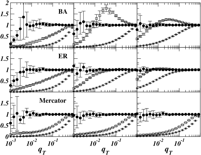
Figure 4: Comparison of the various estimators for the BA (top), ER (middle) and Mercator (bottom) networks. The curves show the ratios of the various estimators to the true network size, as a function of the target density $q_{T}$. Full circles: $\hat{N}_{L1O}/N$ ; Empty squares: $\hat{N}_{RS}/N$; Stars: $N^{*}/N$. Values and one standard deviation error bars are based on 100 trials, with random choice of sources and targets for each trial. Left figures: $n_{S}=1$ source; Middle: $n_{S}=10$ sources; Right: $n_{S}=100$ sources.

The plots in Fig. 4 show a comparison of $N^{*}/N$, $\hat{N}_{RS}/N$, and $\hat{N}_{L1O}/N$, for $n_{S}=1,10,$ and $100$ sources, as a function of $q_{T}$. A value of $1$ for these ratios is desired, and it is clear that in the case of both the resampling and the “leave-one-out” estimator that the improvement over the “trivial” estimator $N^{*}$ is substantial. Increasing either the number of sources $n_{S}$ or the density of targets $q_{T}$ yields better results, even for $N^{*}$, but the estimators we propose converge much faster than $N^{*}$ towards values close to the true size $N$.

Between the resampling and the “leave-one-out” estimator, the latter appears to perform much better. For example, we note that while both estimators suffer from a downward bias for very low values of $q_{T}$, this bias persists into the moderate and, in some cases, even high range for the resampling estimator. This is probably due to the fact that the basic hypothesis of scaling underlying the derivation of $\hat{N}_{RS}$ is only approximately satisfied, while for $\hat{N}_{L1O}$, the underlying hypotheses are indeed well satisfied. Notice, however, that the “leave-one-out” estimator has a larger variability at small values of $q_{T}$, while that of the resampling estimator is fairly constant throughout. This is because the same number $B$ of resamples is used in calculating $\hat{N}_{RS}$ in equation (5), and the uncertainty can be expected to scale similarly, but in calculating $\hat{N}_{L1O}$ in equation (9), the uncertainty will scale with $n_{T}$ (and hence $q_{T}$).

In terms of topology, estimation of $N$ appears to be easiest for the ER model. Even $N^{*}$ is more accurate i.e., the discovery rate is higher. Estimation on the MERCATOR graph appears to be the hardest, although interestingly, the performance of the “leave-one-out” estimator seems to be approximately a function of $N^{*}/N$ and $n_{T}$ and thus quite stable in all three graphs. The MERCATOR graph has a much higher proportion of low-degree vertices than the two synthetic graphs, which therefore have particularly small betweenness (and thus lie on very few shortest paths) and are very difficult to discover. On a side note, we mention too that the resampling estimator behaves in a rather curious, non-monotonic fashion in two of the plots, as $q_{T}$ grows. At the moment, we do not have a reasonable explanation for this behavior, although we note that it appears to be constrained to the case of the BA graph and that some indication of this behavior can already be seen for this graph in Fig. 2.

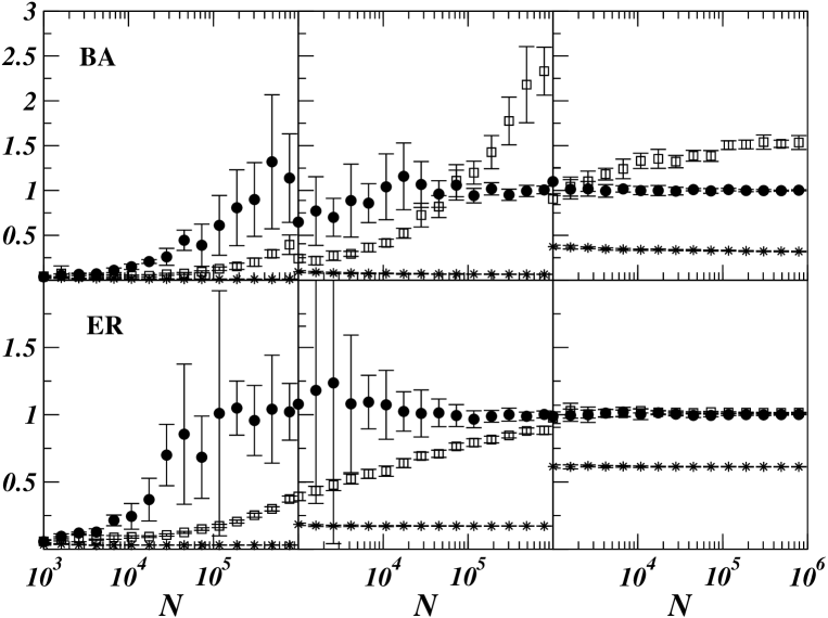
Figure 5: Effect of the size $N$ of the graph $\mathcal{G}$ for BA and ER graphs at constant number of sources and density of targets. The curves show the ratios of the various estimators to the true network size, as a function of the graph size $N$. Full circles: $\hat{N}_{L1O}/N$ ; Empty squares: $\hat{N}_{RS}/N$; Stars: $N^{*}/N$. Values and one standard deviation error bars are based on 100 trials, with random choice of sources and targets for each trial. $n_{S}=10$. Left figures: $q_{T}=10^{-3}$; Middle: $q_{T}=10^{-2}$; Right: $q_{T}=10^{-1}$.

In Fig. 5, we investigate, at fixed $n_{S}$ and $q_{T}$, the effect of the real size of the graph $N$. Interestingly, the estimators perform better for larger sizes, while $N^{*}/N$ on the contrary decreases. This is due to the fact that the sample graph $\mathcal{G}^{*}$ gets bigger, providing more and richer information, even if the discovery ratio does not grow. The odd nature of the results for the BA graph comes from the peak associated with the resampling estimator mentioned earlier; see Fig. 4. At a fixed number $n_{T}$ of targets, however, the quality of the estimators $\hat{N}_{RS}$ and $\hat{N}_{L1O}$ gets worse as $N$ increases, as shown in Fig. 6.

6 Discussion

In this paper, we have investigated the problem of inferring a network’s properties from traceroute-like measurements in the framework of the so-called ‘species’ problem. As a first example of application, we have focused on the issue of estimating the real size $N$ of a network from only the knowledge of the sampled graph. Despite the fact that species problems often can be quite difficult, in this case we find it is possible to propose an estimator that, based on our empirical studies, works quite well, even at quite low sampling densities.

While the present study provides a first promising step that clearly illustrates the relevance of the species problem in Internet inference, numerous issues remain to be explored, even simply in the case of estimation of $N$ alone. For example, the proposed estimators could be evaluated with other types of networks. Similarly, one could examine the effect of non-random source placement (e.g., restricted only to the fringe of the network), as well as that of more realistic traceroute models [32]. However, in the case of these latter two changes, we would not expect the ‘leave-one-out’ estimator to suffer much in performance, since its derivation assumes only uniform random choice of targets, and not sources, and furthermore makes no explicit assumptions about routing. The effect of the inclusion in $\mathcal{G}^{*}$ of the paths from each source to the other sources should as well be investigated.

Our results showed that the ‘leave-one-out’ estimator performed noticeably better than the resampling estimator. Nevertheless, the resampling estimator should not be summarily dismissed quite yet. In particular, while the derivation of the ‘leave-one-out’ estimator is quite specific to the problem of estimating $N$, the derivation of the resampling estimator is general and independent of what is to be estimated. Initial experiments indicate that in estimating the number of edges $M$ in a network, for example, a resampling estimator yields similar improvements over the observed value $M^{*}=|E^{*}|$ as seen in estimating $N$. On the other hand, it is not immediately apparent how the leave-one-out principle might be applied to estimating $M$, as it is nodes (i.e, targets) and not edges that are chosen at the start of a traceroute study.

Finally, it is worth recalling the broader issue raised by this paper: the fact that the problem of estimating a characteristic $\eta(\mathcal{G})$ of a network graph $\mathcal{G}$, based on a sampled subgraph $\mathcal{G}^{*}$, is as yet poorly understood. We have taken the case of $\eta(\mathcal{G})=N$ as a prototype to explore and illustrate. However, for this case alone there are natural alternatives that one might consider. For example, an experiment that used ping to test for the response of some sufficient number $n$ of randomly chosen IP addresses could yield an estimator $\hat{a}$ of the fraction of ‘alive’ addresses and, in turn, an estimator $\hat{N}_{ping}=2^{32}\hat{a}$ that is much simpler than either of those proposed in this paper. We have in fact performed such an experiment, with $n=3,726,773$ ping’s sent from a single source, yielding $61,246$ valid responses (for a $1.64\%$ response rate), and resulting in an estimate $\hat{N}_{ping}=70,583,737$. We then performed a traceroute study from the same source to the $61,216$ unique IP addresses, and calculated a ‘leave-one-out’ estimate on the resulting $G^{*}$ of $\hat{N}_{L1O}=72,296,221$.

Of course, neither of these numbers are intended to be taken too seriously in and of themselves. The point is that, while the estimator from traceroute data is arguably less intuitive and direct in its derivation than that from the ping data, for the particular task of estimating $N$, it nonetheless produces essentially the same number. And, most importantly, while the ping data would of course not be useful for estimating $M$ or degree characteristics, for example, the use of traceroute measurements, which produce an entire sampled subgraph $\mathcal{G}^{*}$, does in principle allow for the estimation of either of these quantities. The success of the ‘leave-one-out’ estimator therefore demonstrates both the importance and the promise of a ‘species’-like perspective in the estimation of Internet characteristics.

Acknowledgements

F.V was funded in part by the ACI Systémes et Sécurité, French Ministry of Research, as part of the MetroSec project. A.B. and L.D. are partially supported by the EU within the 6th Framework Programme under contract 001907 “Dynamically Evolving, Large Scale Information Systems” (DELIS). Part of this work was performed while E.K. was with the LIAFA group at l’Université de Paris-7, with support from the CNRS. This work was supported in part by NSF grants CCR-0325701 and DMS-0405202 and ONR award N000140310043.

Appendix

We derive here the estimator $\hat{N}_{L1O}$ of equation (9). Starting from equation (8), and substituting $\bar{N}^{*}_{(-)}$ and $X$ in the numerator for $E[N^{*}_{(-)}]$ and $E[X]$, respectively, our task reduces to deriving an estimator of $(n_{T}-E[X])^{-1}=(n_{T}q)^{-1}$, where $q=1-(E[X]/n_{T})$.

Recall that $X=\sum_{j}\delta_{j}$ is the sum of $n_{T}$ Bernoulli (i.e., 0 or 1) random variables. If the $\delta_{j}$ were independent and identically distributed (i.i.d.), with $\Pr(\delta_{j}=1)=p$, then $X$ would be a binomial random variable, with parameters $n_{T}$ and $p$. In this case, the relation $qE[(n_{T}+1)/(n_{T}+1-X)]=1-p^{n+1}$ holds, from which it follows that the quantity $(n_{T}+1)/(n_{T}+1-X)$ has expectation $q^{-1}(1-p^{n+1})\approx q^{-1}$, and therefore is an approximately unbiased estimator of $q^{-1}$. Substitution of the quantity $(n_{T}+1)/[n_{T}(n_{T}+1-X)]$ for $(n_{T}q)^{-1}=(n-E[X])^{-1}$ in (8) then completes the derivation of (9).

Of course, the variables $\delta_{j}$ are not precisely i.i.d., due to the commonality of sources and targets underlying the definition of the sets $\mathcal{V}^{*}_{(-j)}$. However, the $\delta_{j}$ share the same marginal distribution (i.e., with $p=(N-E[N^{*}_{(-)}])/(N-n_{S}-n_{T}+1)$  ), and it may be argued that they are pairwise nearly independent under the condition $N^{*}_{(-j)}\approx N^{*}_{(-j^{\prime})}\approx N^{*}_{(-j,-j^{\prime})}$. These two facts together suggest that a binomial approximation to the distribution of $X$ should be quite accurate. It remains to argue for the latter fact, for which it is sufficient to show that $\Pr(\delta_{j}=0|\delta_{j^{\prime}}=0)\approx\Pr(\delta_{j}=0)=1-p$. By conditioning on the sets $\mathcal{V}^{*}_{(-j)}$ and $\mathcal{V}^{*}_{(-j^{\prime})}$, counting arguments similar to those underlying the derivation of equation (6) yield that

$$\Pr(\delta_{j}=0|\delta_{j^{\prime}}=0) = E\left[\frac{N^{*}_{(-j)}-1}{N-m-n+1}\,\cdot\,\frac{N^{*}_{(-j,-j^{\prime})}}{N^{*}_{(-j^{\prime})}}\,+\,\frac{N^{*}_{(-j)}}{N-m-n+1}\,\cdot\,\frac{N^{*}_{(-j^{\prime})}-N^{*}_{(-j,-j^{\prime})}}{N^{*}_{(-j^{\prime})}}\right]$$

$$\approx E\left[\frac{N^{*}_{(-j)}-1}{N-m-n+1}\,\cdot\,1\,+\,\frac{N^{*}_{(-j)}}{N-m-n+1}\,\cdot\,0\right]\,\approx\,1-p\enskip.$$

Figure 1: Illustration of the traceroute-like procedure. Shortest paths between the set of sources and the set of destination targets are discovered (shown in full lines) while other edges are not found (dashed lines). In the case of degenerate shortest paths, only one is found.

Figure 6: Effect of the size $N$ of the graph $\mathcal{G}$ for BA and ER graphs at constant number of sources and targets. The curves show the ratios of the various estimators to the true network size, as a function of the graph size $N$. Full circles: $\hat{N}_{L1O}/N$ ; Empty squares: $\hat{N}_{RS}/N$; Stars: $N^{*}/N$. Values and one standard deviation error bars are based on 100 trials, with random choice of sources and targets for each trial. $n_{S}=10$. Left figures: $n_{T}=10^{2}$ targets; Middle: $n_{T}=10^{3}$ targets; Right: $n_{T}=10^{4}$ targets.

References

- [1] S. N. Dorogovtsev and J. F. F. Mendes, Evolution of networks: From biological nets to the Internet and WWW (Oxford University Press, Oxford, 2003).
- [2] R. Pastor-Satorras and A. Vespignani, Evolution and structure of the Internet: A statistical physics approach (Cambridge University Press, Cambridge, 2004).
- [3] The National Laboratory for Applied Network Research (NLANR), sponsored by the National Science Foundation. (see http://moat.nlanr.net/).
- [4] The Cooperative Association for Internet Data Analysis (CAIDA), located at the San Diego Supercomputer Center. (see http://www.caida.org/home/).
- [5] Topology project, Electric Engineering and Computer Science Department, University of Michigan (http://topology.eecs.umich.edu/).
- [6] SCAN project at the Information Sciences Institute (http://www.isi.edu/div7/scan/).
- [7] Internet mapping project at Lucent Bell Labs (http://www.cs.bell-labs.com/who/ches/map/).
- [8] M. Faloutsos, P. Faloutsos, and C. Faloutsos, On Power-law Relationships of the Internet Topology, ACM SIGCOMM ’99, Comput. Commun. Rev. , 251–262 (1999).
- [9] A. Lakhina, J. W. Byers, M. Crovella and P. Xie, Sampling Biases in IP Topology Measurements, Technical Report BUCS-TR-2002-021, Department of Computer Sciences, Boston University (2002).
- [10] A. Clauset and C. Moore, Accuracy and Scaling Phenomena in Internet Mapping, Phys. Rev. Lett. 94, 018701 (2005).
- [11] T. Petermann and P. De Los Rios, Exploration of Scale-Free Networks - Do we measure the real exponents?, Eur. Phys. J. B 201-204 (2004).
- [12] L. Dall’Asta, I. Alvarez-Hamelin, A. Barrat, A. Vázquez, A. Vespignani, Statistical theory of Internet exploration, Phys. Rev. E 71 (2005) 036135. L. Dall’Asta, I. Alvarez-Hamelin, A. Barrat, A. Vázquez, A. Vespignani, Exploring networks with traceroute-like probes: theory and simulations, to appear in Theoretical Computer Science.
- [13] D. Achlioptas, A. Clauset, D. Kempe and C. Moore, On the Bias of Traceroute Sampling; or, Power-law Degree Distributions in Regular Graphs, cond-mat/0503087, to appear in STOC 2005.
- [14] J.-L. Guillaume and M. Latapy, Relevance of Massively Distributed Explorations of the Internet Topology: Simulation Results, IEEE Infocom’05, 2005, Miami, USA.
- [15] H. Burch and B. Cheswick, Mapping the internet, IEEE computer, , 97–98 (1999).
- [16] W.W. Esty, Estimation of the Size of a Coinage: A Survey and Comparison of Methods, Numismatic Chronicle, , 185-215 (1986).
- [17] D. McNeil, Estimating an Author’s Vocabulary, Journal of the American Statistical Association, , 92-96 (1973).
- [18] B. Efron and R. Thisted, Estimating the Number of Unseen Species: How Many Words Did Shakespeare Know?, Biometrika, , 435-447 (1976).
- [19] J. Bunge and M. Fitzpatrick, Estimating the Number of Species: A Review, Journal of the American Statistical Association, , 364-373 (1993).
- [20] C.-H. Zhang, Estimation of sums of random variables: examples and information bounds, Annals of Statistics, 33, (2005).
- [21] K.-I. Goh, B. Kahng and D. Kim, Packet transport and load distribution in scale-free network models, Physica A , 72 (2003).
- [22] G. McLachlan and D. Peel, Finite Mixture Models, New York, New York: John Wiley & Sons, Inc., 2000.
- [23] I.J. Good, On the population frequencies of species and the estimation of population parameters, Biometrika, 40, 237 264 (1953).
- [24] H. Robbins and C.-H. Zhang, Efficiency of the u, v method of estimation, Proc. Natl. Acad. Sci. USA, 97, 12976 -12979 (2000).
- [25] B. Efron, The jackknife, the bootstrap, and other resampling plans, Society of Industrial and Applied Mathematics CBMS-NSF Monographs, 38 (1982).
- [26] G. Quenouille, Notes on bias in estimation, Biometrika, 43, 353-360 (1956).
- [27] J.W. Tukey, Bias and confidence in not quite large samples, Annals of Mathematical Statistics, 29, 614 (1958).
- [28] P. Barford, A. Bestavros, J. Byers, and M. Crovella, On the Marginal Utility of Network Topology Measurements, Proc. ACM SIGCOMM Internet Measurement Workshop, 2001.
- [29] P. Erdös and P. Rényi, On random graphs I, Publ. Math. Debrecen 6, 290 (1959).
- [30] A.-L. Barabási and R. Albert, Emergence of scaling in random networks, Science , 509–512 (1999).
- [31] R. Govindan and H. Tangmunarunkit, Heuristics for Internet Map Discovery, Proc. IEEE INFOCOM, pp 1371-1380, 2000.
- [32] J. Leguay, M. Latapy, T. Friedman and K. Salamatian, Describing and Simulating Internet Routes, preprint cs.NI/0411051.