Taylor series expansions for the entropy rate of Hidden Markov Processes

Abstract

Finding the entropy rate of Hidden Markov Processes is an active research topic, of both theoretical and practical importance. A recently used approach is studying the asymptotic behavior of the entropy rate in various regimes. In this paper we generalize and prove a previous conjecture relating the entropy rate to entropies of finite systems. Building on our new theorems, we establish series expansions for the entropy rate in two different regimes. We also study the radius of convergence of the two series expansions.

I Introduction

Let $\{X_{N}\}$ be a finite state stationary markov process over the alphabet $\Sigma=\{1,\ldots,s\}$. Let $\{Y_{N}\}$ be its noisy observation (on the same alphabet). Let $M=M_{s\times s}=\{m_{ij}\}$ be the Markov transition matrix and $R=R_{s\times s}$ be the emission matrix, i.e. $P(X_{N+1}=j|X_{N}=i)=m_{ij}$ and $P(Y_{N}=j|X_{N}=i)=r_{ij}$. We assume that the Markov matrix $M$ is strictly positive ($m_{ij}>0$), and denote its stationary distribution by the (column) vector $\pi$ ,satisfying $\pi^{t}M=\pi^{t}$.

The process $Y$ can be viewed as a noisy observation of $X$, through a noisy channel. It is known as a Hidden Markov Process (HMP), and is determined by the parameters $M$ and $R$. More generally, HMPs have a rich and developed theory, and enourmous applications in various fields (see [1, 2]).

An important property of the process $Y$ is its entropy rate. The Shannon entropy rate of a stochastic process ([3]) measures the amount of ’uncertainty per-symbol’. More formally, for $i\leq j$, let $[X]_{i}^{j}$ denote the vector $(X_{i},\ldots,X_{j})$. Then the entropy rate $\bar{H}(Y)$ is defined as :

$$\bar{H}(Y)=\lim_{N\to\infty}\frac{H([Y]_{1}^{N})}{N}$$ (1)

Where $H(X)=-\sum_{X}P(X)\log P(X)$; Here and throughout the paper we use natural logarithms, so the entropy is measured in NATS, and also adopt the convention $0\log 0\equiv 0$. We sometimes omit the realization $x$ of the variable $X$, so $P(X)$ should be understood as $P(X=x)$. The entropy rate can also be computed via the conditional entropy as: $\bar{H}(Y)=\lim_{N\to\infty}H(Y_{N}|[Y]_{1}^{N-1})$, since for a stationary process the two limits exist and coincide ([4]). The conditional entropy $H(Y|X)$ (where $X,Y$ are sets of r.v.s.) represents the average uncertainty of $Y$, assuming that we know $X$, that is $H(Y|X)=\sum_{x}P(X=x)H(Y|X=x)$. By the chain rule for entropy, it can also be viewed as a difference of entropies, $H(Y|X)=H(X,Y)-H(X)$, which will be used later.

There is at present no explicit expression for the entropy rate of a HMP ([1, 5]). Few recent works ([5, 6, 7]) have dealt with finding the asymptotic behavior of $\bar{H}$ in several parameter regimes. However, they concentrated only on binary alphabet, and proved rigorously only bounds or at most second ([7]) order behavior.

Here we generalize and prove a conjecture posed in [7], which justifies (under some mild assumptions) the computation of $\bar{H}$ as a series expansion in the High Signal-to-Noise-Ratio (’High-SNR’) regime. The expansion coefficients were given in [7], for the symmetric binary case. In this case, the matrices $M$ and $R$ are given by :

$$M=\begin{pmatrix}1-p&p\\ p&1-p\end{pmatrix}\>\>,\>\>R=\begin{pmatrix}1-\epsilon&\epsilon\\ \epsilon&1-\epsilon\end{pmatrix}$$

and the process is characterized by the two parameters $p,\epsilon$. The High-SNR expansion in this case is an expansion in $\epsilon$ around zero.

In section II, we present and prove our two main theorems; Thm. 3 is a generalization of a conjecture raised in [7] which connects the coefficients of entropies using finite histories to the entropy rate. Proving it justifies the High-SNR expansion of [7]. We also give Thm. 2, which is the analogous of Thm. 3 in a different regime, termed ’Almost-Memoryless’ (’A-M’).

In section III we use our two new theorems to compute the first coefficients in the series expansions for the two regimes. We give the first-order asymptotics for a general alphabet, as well as higher order coefficients for the symmetric binary case.

In section IV we estimate the radius of convergence of our expansions using a finite number of terms, and compare our results for the two regimes. We end with conclusions and future directions.

II From Finite system entropy to entropy rate

In this section we prove our main results, namely Thms. 3 and 2, which relate the coefficients of the finite bounds $C_{N}$ to those of the entropy rate $\bar{H}$ in two different regimes.

II-A The High SNR Regime

This regime was dealt in further details in [7, 8], albeit with no rigorous justification for the obtained series expansion. In the High-SNR regime the observations are likely to be equal to the states, or in other words, the emission matrix $R$ is close to the identity matrix $I$. We therefore write $R=I+\epsilon T$, where $\epsilon>0$ is a small constant and $T=\{t_{ij}\}$ is a matrix satisfying $t_{ii}<0,\>t_{ij}\geq 0,\>\forall i\neq j$ and $\sum_{j=1}^{s}{t_{ij}}=0$. The entropy rate in this regime can be given as an expansion in $\epsilon$ around zero. We state here our new theorem, connecting the entropy of finite systems to the entropy rate in this regime.

Theorem 1

Let $H_{N}\equiv H_{N}(M,T,\epsilon)=H([Y]_{1}^{N})$ be the entropy of a finite system of length $N$, and let $C_{N}=H_{N}-H_{N-1}$. Assume that there is some (complex) neighborhood $B_{\rho}(0)=\{\epsilon:|\epsilon|<\rho\}\subset\mathbb{C}$ of $\epsilon=0$, in which the (one-variable) functions $\{C_{N}\},\bar{H}$ are analytic in $\epsilon$, with a Taylor expansion given by :

$$C_{N}(M,T,\epsilon)=\sum_{k=0}^{\infty}C_{N}^{(k)}\epsilon^{k},\quad\bar{H}(M,T,\epsilon)=\sum_{k=0}^{\infty}C^{(k)}\epsilon^{k}$$ (2)

(The coefficients $C_{N}^{(k)}$ are functions of the parameters $M$ and $T$. From now on we omit this dependence). Then:

$$N\geq\lceil\frac{k+3}{2}\rceil\Rightarrow C_{N}^{(k)}=C^{(k)}$$ (3)

The recent result ([9]) on analyticity of $\bar{H}$ is not applicable near $\epsilon=0$, therefore the analytic domain of $C_{N}$, and, more importantly $\bar{H}$, will be discussed elsewhere.

$C_{N}$ is actually an upperbound ([4]) for $\bar{H}$. The behavior stated in Thm. 3 was discovered previously using symbolic computations, but was proven only for $k\leq 2$ , and only for the symmetric binary case (see [7]).

Although technically involved , the proof of Thm. 3 is based on the following two simple ideas. First, we distinguish between the noise parameters at different sites. This is done by considering a more general process $\{Z_{N}\}$, where $Z_{i}$’s emission matrix is $R_{i}=I+\epsilon_{i}T$. The joint distribution of $[Z]_{1}^{N}$ is thus determined by $M$,$T$ and $[\epsilon]_{1}^{N}$. We define the following functions :

$$F_{N}(M,T,[\epsilon]_{1}^{N})=H([Z]_{1}^{N})-H([Z]_{1}^{N-1})$$ (4)

Setting all the $\epsilon_{i}$’s equal, reduces us back to the $Y$ process, so in particular $F_{N}(M,T,(\epsilon,\ldots,\epsilon))=C_{N}(\epsilon)$.

Second, we observe that if a particular $\epsilon_{i}$ is set to zero, the corresponding observation $Z_{i}$ must equal the state $X_{i}$. Thus, conditioning back to the past is ’blocked’. This can be used to prove the following :

Lemma 1

Assume $\epsilon_{j}=0$ for some $1<j<N$. Then :

$$F_{N}([\epsilon]_{1}^{N})=F_{N-j+1}([\epsilon]_{j+1}^{N})$$

Proof:

$F$ can be written as a sum of conditional entropies :

$$F_{N}=-\sum_{[Z]_{1}^{N}}P([Z]_{1}^{N-1})P(Z_{N}|[Z]_{1}^{N-1})\log P(Z_{N}|[Z]_{1}^{N-1})$$ (5)

Where the dependence on $[\epsilon]_{1}^{N}$ and $M,T$ comes through the probabilities $P(..)$. Since $\epsilon_{j}=0$, we must have $X_{j}=Z_{j}$, and therefore (since the $X_{i}$’s form a Markov chain), conditioning further to the past is ’blocked’, that is :

$$\epsilon_{j}=0\Rightarrow P(Z_{N}|[Z]_{1}^{N-1})=P(Z_{N}|[Z]_{j}^{N-1})$$ (6)

(Note that eq. (6) is true for $j<N$, but not for $j=N$). Substituting in eq. (5) gives :

$$F_{N}=-\sum_{[Z]_{1}^{N}}P([Z]_{1}^{N-1})P(Z_{N}|[Z]_{j}^{N-1})\log P(Z_{N}|[Z]_{j}^{N-1})=$$

$$-\sum_{Z_{j}^{N}}P([Z]_{j}^{N-1})P(Z_{N}|[Z]_{j}^{N-1})\log P(Z_{N}|[Z]_{j}^{N-1})$$

$$=F_{N-j+1}$$ (7)

 

Let $\vec{k}=[k]_{1}^{N}$ be a vector with $k_{i}\in\{\mathbb{N}\cup 0\}$. Define its ’weight’ as $\omega(\vec{k})=\sum_{i=1}^{N}k_{i}$. Define also :

$$F_{N}^{\vec{k}}\equiv\left.\frac{\partial^{\omega(\vec{k})}F_{N}}{\partial\epsilon_{1}^{k_{1}},\ldots,\partial\epsilon_{N}^{k_{N}}}\right|_{\vec{\epsilon}=0}$$ (8)

The next lemma shows that adding zeros to the left of $\vec{k}$ leaves $F_{N}^{\vec{k}}$ unchanged :

Lemma 2

Let $\vec{k}=[k]_{1}^{N}$ with $k_{1}\leq 1$. Denote $\vec{k}^{(r)}$ the concatenation of $\vec{k}$ with $r$ zeros : $\vec{k}^{(r)}=(\underbrace{0,\ldots,0}_{r},k_{1},\ldots,k_{N})$. Then :

$$F_{N}^{\vec{k}}=F_{r+N}^{\vec{k}^{(r)}}\quad,\forall r\in\mathbb{N}$$

Proof:

Assume first $k_{1}=0$. Using lemma 1, we get :

$$F_{N+r}^{\vec{k}^{(r)}}([\epsilon]_{1}^{N+r})=\left.\frac{\partial^{\omega(\vec{k}^{(r)})}F_{r+N}([\epsilon]_{1}^{N+r})}{\partial\epsilon_{r+2}^{k_{2}},\ldots,\partial\epsilon_{r+N}^{k_{N}}}\right|_{\vec{\epsilon}=0}=$$

$$\left.\frac{\partial^{\omega(\vec{k})}F_{N}([\epsilon]_{r+1}^{N+r})}{\partial\epsilon_{r+2}^{k_{2}},\ldots,\partial\epsilon_{r+N}^{k_{N}}}\right|_{\vec{\epsilon}=0}=F_{N}^{\vec{k}}([\epsilon]_{r+1}^{r+N})$$ (9)

The case $k_{1}=1$ is reduced back to the case $k_{1}=0$ by taking the derivative. We denote by ${[Z]_{1}^{N}}^{(j\to r)}$ the vector which is equal to $[Z]_{1}^{N}$ in all coordinates except on coordinate $j$, where $Z_{j}=r$. Using eq. (9), we get :

$$F_{N+1}^{\vec{k}^{(1)}}([\epsilon]_{1}^{N+1})=\left.\frac{\partial^{\omega(\vec{k})-1}}{\partial\epsilon_{3}^{k_{2}}\dots\partial\epsilon_{N+1}^{k_{N}}}\left[\left.\frac{\partial F_{N+1}}{\partial\epsilon_{2}}\right|_{\epsilon_{2}=0}\right]\right|_{\vec{\epsilon}=0}=$$

$$\frac{\partial^{\omega(\vec{k})-1}}{\partial\epsilon_{3}^{k_{2}}\dots\partial\epsilon_{N+1}^{k_{N}}}\Biggl{\{}-\sum_{r=1}^{s}t_{X_{i}r}\sum_{[Z]_{1}^{N+1}}$$

$$\left[P({[Z]_{1}^{N+1}}^{(2\to r)})\log P(Z_{N+1}|[Z]_{1}^{N})-\right.$$

$$\left.\left.\left.P(Z_{N+1}|[Z]_{1}^{N})P({[Z]_{1}^{N}}^{(2\to r)})\right]\right|_{\epsilon_{2}=0}\Biggr{\}}\right|_{[\epsilon]_{1}^{N+1}=0}=$$

$$\frac{\partial^{\omega(\vec{k})-1}}{\partial\epsilon_{2}^{k_{2}}\dots\partial\epsilon_{N}^{k_{N}}}\Biggl{\{}-\sum_{r=1}^{s}t_{X_{i}r}\sum_{[Z]_{1}^{N}}$$

$$\left[P({[Z]_{1}^{N}}^{(1\to r)})\log P(Z_{N}|[Z]_{1}^{N-1})-\right.$$

$$\left.\left.\left.P(Z_{N}|[Z]_{1}^{N-1})P({[Z]_{1}^{N}}^{(1\to r)})\right]\right|_{\epsilon_{1}=0}\Biggr{\}}\right|_{[\epsilon]_{1}^{N}=0}=F_{N}^{\vec{k}}([\epsilon]_{1}^{N})$$ (10)

 

$C_{N}^{(k)}$ is obtained by summing $F_{N}^{\vec{k}}$ on all $\vec{k}$’s with weight $k$ :

$$C_{N}^{(k)}=\sum_{\vec{k},\omega(\vec{k})=k}F_{N}^{\vec{k}}$$ (11)

We now show that one does not need to sum on all such $\vec{k}$’s, as many of them give zero contribution :

Lemma 3

Let $\vec{k}=(k_{1},\ldots,k_{N})$. If $\exists i<j<N$, with $k_{i}\geq 1,k_{j}\leq 1$, then $F_{N}^{\vec{k}}=0$.

Proof:

Assume first $k_{j}=0$. Using lemma 1 we get

$$F_{N}^{\vec{k}}\equiv\left.\frac{\partial^{\omega(\vec{k})}F_{N}(\vec{\epsilon})}{\partial\epsilon_{1}^{k_{1}},\ldots,\partial\epsilon_{N}^{k_{N}}}\right|_{\vec{\epsilon}=0}=\left.\frac{\partial^{\omega(\vec{k})}F_{N-j+1}([\epsilon]_{j}^{N})}{\partial\epsilon_{1}^{k_{1}},\ldots,\partial\epsilon_{N}^{k_{N}}}\right|_{\vec{\epsilon}=0}=$$

$$\frac{\partial^{\omega(\vec{k})-1}}{\partial\epsilon_{1}^{k_{1}},\ldots,\partial\epsilon_{i}^{k_{i}-1},\ldots,\partial\epsilon_{N}^{k_{N}}}\left[\left.\frac{\partial F_{N-j+1}([\epsilon]_{j}^{N})}{\partial\epsilon_{i}}\right]\right|_{\vec{\epsilon}=0}=0$$ (12)

The case $k_{j}=1$ is more difficult, but follows the same principles. Write the probability of $Z$ :

$$P([Z]_{1}^{N})=\sum_{[X]_{1}^{N}}P([X]_{1}^{N})P([Z]_{1}^{N}|[X]_{1}^{N})=$$

$$\sum_{[X]_{1}^{N}}P([X]_{1}^{N})\prod_{i=1}^{N}(\delta_{X_{i}Z_{i}}+\epsilon_{i}t_{X_{i}Z_{i}})$$ (13)

where $\delta_{ij}$ is Kronecker delta. Write now the derivative with respect to $\epsilon_{j}$:

$$\left.\frac{\partial P([Z]_{1}^{N})}{\partial\epsilon_{j}}\right|_{\epsilon_{j}=0}=$$

$$\left.\sum_{[X]_{1}^{N}}\left[P([X]_{1}^{N})t_{X_{j}Z_{j}}\prod_{i\neq j}(\delta_{X_{i}Z_{i}}+\epsilon_{i}t_{X_{i}Z_{i}})\right]\right|_{\epsilon_{j}=0}=$$

$$\left.\left\{\sum_{r=1}^{s}t_{X_{i}r}P({[Z]_{1}^{N}}^{(j\to r)})\right\}\right|_{\epsilon_{j}=0}$$ (14)

Using Bayes’ rule $P(Z_{N}|[Z]_{1}^{N-1})=\frac{P([Z]_{1}^{N})}{P([Z]_{1}^{N-1})}$, we get :

$$\left.\frac{\partial P(Z_{N}|[Z]_{1}^{N-1})}{\partial\epsilon_{j}}\right|_{\epsilon_{j}=0}=$$

$$\frac{1}{P([Z]_{1}^{N-1})}\sum_{r=1}^{s}t_{X_{i}r}\left[P({[Z]_{1}^{N}}^{(j\to r)})-\right.$$

$$\left.\left.P(Z_{N}|[Z]_{1}^{N-1})P({[Z]_{1}^{N-1}}^{(j\to r)})\right]\right|_{\epsilon_{j}=0}$$ (15)

This gives :

$$\left.\frac{\partial[P([Z]_{1}^{N})\log P(Z_{N}|[Z]_{1}^{N-1})]}{\partial\epsilon_{j}}\right|_{\epsilon_{j}=0}=$$

$$\sum_{r=1}^{s}t_{X_{i}r}\left\{P({[Z]_{1}^{N}}^{(j\to r)})\log P(Z_{N}|[Z]_{1}^{N-1})+\right.$$

$$\left.\left.P({[Z]_{1}^{N}}^{(j\to r)})-P(Z_{N}|[Z]_{1}^{N-1})P({[Z]_{1}^{N-1}}^{(j\to r)})\right\}\right|_{\epsilon_{j}=0}$$ (16)

And therefore :

$$\left.\frac{\partial F_{N}}{\partial\epsilon_{j}}\right|_{\epsilon_{j}=0}=$$

$$-\sum_{r=1}^{s}t_{X_{i}r}\Biggl{\{}\sum_{[Z]_{1}^{N}}\left[P({[Z]_{1}^{N}}^{(j\to r)})\log P(Z_{N}|[Z]_{1}^{N-1})-\right.$$

$$\left.\left.P(Z_{N}|[Z]_{1}^{N-1})P({[Z]_{1}^{N-1}}^{(j\to r)})\right]\Biggr{\}}\right|_{\epsilon_{j}=0}=$$

$$\Biggl{\{}-\sum_{r=1}^{s}t_{X_{i}r}\sum_{[Z]_{j}^{N}}\left[P({[Z]_{j}^{N}}^{(1\to r)})\log P(Z_{N}|[Z]_{j}^{N-1})-\right.$$

$$\left.\left.P(Z_{N}|[Z]_{j}^{N-1})P({[Z]_{j}^{N-1}}^{(1\to r)})\right]\Biggr{\}}\right|_{\epsilon_{1}=0}$$ (17)

Where the latter equality comes from using eq. (6), which ’blocks’ the dependence backwards. Eq. 17 shows that $\left.\frac{\partial F_{N}}{\partial\epsilon_{j}}\right|_{\epsilon_{j}=0}$ does not depend on $\epsilon_{i}$ for $i<j$, therefore $\frac{\partial^{k_{i}+1}F_{N}}{\partial\epsilon_{i}^{k_{i}}\partial\epsilon_{j}}=0$ and $F_{N}^{\vec{k}}=0$.

 

We are now ready to prove Thm. 3, which follows directly from lemmas 2 and 3 :

Proof:

Let $\vec{k}=[k]_{1}^{N}$ with $\omega(\vec{k})=k$. Define its ’length’ (from right, considering only entries larger than one) as $l(\vec{k})=N+1-\min_{k_{i}>1}\{i\}$. It easily follows from lemma 3 that if $F_{N}^{\vec{k}}\neq 0$, we must have $l(\vec{k})\leq\lceil\frac{k+3}{2}\rceil-1$. Therefore, according to lemma 2 we have :

$$F_{N}^{\vec{k}}=F_{\lceil\frac{k+3}{2}\rceil}^{(k_{N-\lceil\frac{k+3}{2}\rceil+1},\ldots,{k_{N}})}$$ (18)

for all $\vec{k}$’s in the sum. Summing on all $F_{N}^{\vec{k}}$ with the same ’weight’, we get $C_{N}^{(k)}=C_{\lceil\frac{k+3}{2}\rceil}^{(k)},\quad\forall N>\lceil\frac{k+3}{2}\rceil$. From the analyticity of $C_{N}$ and $\bar{H}$ around $\epsilon=0$, one can show by induction that $\lim_{N\to\infty}C_{N}^{(k)}=C^{(k)}$, therefore we must have $C_{N}^{(k)}=C^{(k)},\quad\forall N\geq\lceil\frac{k+3}{2}\rceil$.

 

II-B The Almost Memoryless Regime

In the A-M regime, the Markov transition matrix is close to uniform. Thus, throughout this section, we assume that $M$ is given by $M=U+\delta T$, such that $U$ is a constant (uniform) matrix, $u_{ij}=s^{-1}$, $\delta>0$ is a small constant and $T$ satisfies $\sum_{j=1}^{s}{t_{ij}}=0$. Thus the process is entirely characterized by the set of parameters $(R,T,\delta)$, where $R$ again denotes the emission matrix.

Interestingly, similarly to the High-SNR regime, the conditional entropy given a finite history gives the correct entropy rate up to a certain order which depends on the finite history taken. In the A-M regime we can also prove analyticity of $\{C_{N}\}$ and $\bar{H}$ in $\delta$ near $\delta=0$. This is stated as :

Theorem 2

Let $H_{N}\equiv H_{N}(R,T,\delta)=H([Y]_{1}^{N})$ be the entropy of a finite system of length $N$, and let $C_{N}=H_{N}-H_{N-1}$. Then :

1. There is some (complex) neighborhood $B_{\rho}(0)=\{\delta:|\delta|<\rho\}\subset\mathbb{C}$ of $\delta=0$, in which the (one-variable) functions $\{C_{N}\},\bar{H}$ are analytic in $\delta$, with a Taylor expansion denoted by :

   $$C_{N}(M,T,\delta)=\sum_{k=0}^{\infty}C_{N}^{(k)}\delta^{k},\quad\bar{H}(M,T,\epsilon)=\sum_{k=0}^{\infty}C^{(k)}\delta^{k}$$ (19)

   (The coefficients $C_{N}^{(k)}$ are functions of the parameters $M$ and $T$.)

2. With the above notations :

   $$N\geq\lceil\frac{k+3}{2}\rceil\Rightarrow C_{N}^{(k)}=C^{(k)}$$ (20)

Proof:

1. The proof of analyticity relies on the recent result, namely Thm. 1.1 in [9]. In order to use this result, we need to present the HMP $Y$ in the following way : We introduce the new alphabet $\Gamma\subset\Sigma\times\Sigma$ defined by :

   $$\Gamma=\Big{\{}w=(w_{x},w_{y}):w_{x},w_{y}\in\Sigma,r_{w_{x}w_{y}}>0\Big{\}}$$

   We also introduce the function $\Phi:\Gamma\to\Sigma$, defined by $\Phi(w)\equiv\Phi(w_{x},w_{y})=w_{y}$. Let $w,v\in\Gamma$ with $w=(w_{x},w_{y}),v=(v_{x},v_{y})$. One can look at the new Markov process $W=(X,Y)$, defined on $\Gamma$ by the transition matrix $\Delta_{|\Gamma|\times|\Gamma|}$, which is given by $\Delta_{wv}\equiv P(W_{N+1}=v|W_{N}=w)=m_{w_{x}v_{x}}r_{v_{x}v_{y}}$. Then the process $Y$ can be defined as $Y_{N}=\Phi(W_{N})$. Using the above representation, clearly $\Delta$ is analytically parameterized by $\delta$. Moreover, there is some (real) neighborhood $B_{\rho^{\prime}}(0)\subset\mathbb{R}$ in which all of $\Delta$’s entries are positive. Therefore, Thm. 1.1 from [9] applies here, and according to its proof, $\{C_{N}\}$ and $\bar{H}$ are analytic (as functions of $\delta$) in some complex neighborhood $B_{\rho}(0)\subset\mathbb{C}$ of zero.

2. The proof of part 2 is very similar to that of Thm. 3. Distinguishing between the sites by setting $M_{i}=U+\delta_{i}T$ in site $i$, we notice that if one sets $\delta_{i}=0$ for some $i$, then $M_{i}$ becomes uniform, and thus knowing $Z_{i}$ ’blocks’ the dependence of $Z_{N}$ on previous $Z_{j}$’s ($\forall j<i$). The rest of the proof continues in an analogous way to the proof of Thm. 3 (including the three lemmas therein), and its details are thus omitted here.

 

III Computation of the series coefficients

An immediate application of Thms. 3 and 2 is the computation of the first terms in the series expansion for $\bar{H}$ (assuming its existance), by simply computing these terms for $C_{N}$ for $N$ large enough. In this section we compute, for both regimes, the first order for the general alphabet case, and also give few higher order terms for the simple symmetric binary case. Our method for computing $C^{(k)}$ is straightforward. We compute $C_{N}^{(k)}$ for $N=\lceil\frac{k+3}{2}\rceil$ by simply enumerating all sequences $[Y]_{1}^{N}$, computing the $k$-th coefficient in $P([Y]_{1}^{N})\log P([Y]_{1}^{N})$ for each one, and summing their contribution. This computation is, however, exponential in $k$, and thus raises the challenge of designing more efficient algorithms, in order to compute further orders and for larger alphabets.

Before giving the calculated coefficients, we need some new notations. For a vector $\alpha$, $diag(\alpha)$ denotes the square matrix with $\alpha$’s elements on the diagonal. We use Matlab-like notation to denote element-by-element operations on matrices. Thus, for matrices $A$ and $B$, $logA$ is a matrix whose elements are $\{\log a_{ij}\}$, and $[A.*B]$ is a matrix whose elements are $\{a_{ij}b_{ij}\}$. $\xi$ denotes the (column) vector of $N$ ones.

III-A The High-SNR expansion

According to Thm. 3, computing $C_{2}$ enables us to extract $\bar{H}^{(k)}$. This is used to show the following :

Proposition 1

Let $R=I+\epsilon T$. Assume that the entropy rate $\bar{H}$ is analytic in some neighborhood of $\delta=0$. Then $\bar{H}$ satisfies :

$$\bar{H}=-\pi^{t}[M.*\log M]\xi+\xi^{t}\Bigl{\{}diag(\log(\pi))T^{t}diag(\pi)M-$$

$$[diag(\pi)MT+T^{t}diag(\pi)M].*[\log(diag(\pi)M)]\Bigr{\}}\xi\epsilon+O(\epsilon^{2})$$ (21)

Proof:

Noting that according to Thm. 3, $\bar{H}=C_{2}+O(\epsilon^{2})$, we first compute (exactly) $C_{2}$, and then expand it by substituting $R=I+\epsilon T$. Write $C_{2}$ as :

$$C_{2}=H(Y_{N}|Y_{N-1})=$$

$$-\sum_{i,j}P(Y_{N}=j,Y_{N-1}=i)\log\frac{P(Y_{N}=j,Y_{N-1}=i)}{P(Y_{N-1}=i)}$$ (22)

We can express the above probabilities as :

$$P(Y_{N-1}=i)=[\pi R]_{i}$$

$$P(Y_{N}=j,Y_{N-1}=i)=[R^{t}diag(\pi)MR]_{ij}\equiv F_{ij}$$ (23)

Substituting eq. (23) in eq. (22), and writing in matrix form, we get :

$$C_{2}=\Bigl{\{}[log(\pi R)]F-\xi^{T}[F.*logF]\Bigr{\}}\xi$$ (24)

Substituting $R=I+\epsilon T$ gives :

$$F=diag(\pi)M+[diag(\pi)MT+T^{t}diag(\pi)M]\epsilon+O(\epsilon^{2}),$$

$$F.*\log F=[diag(\pi)M].*\log(diag(\pi)M)+$$

$$\Bigl{\{}[diag(\pi)MT+T^{t}diag(\pi)M].*[I+\log(diag(\pi)M)]\Bigr{\}}\epsilon+$$

$$O(\epsilon^{2})$$ (25)

Substituting these in eq. (24) gives, after simplification, the result (21).

 

We note that prop. 1 above is a generalization of the result obtained by [5] for a binary alphabet.

Turning now into the symmetric binary case, the first eleven orders of the series expansion were given in [7], but only the first two were proved to be correct. Thm. 3 proves the correctness of the entire expansion from [7] (under the analyticity assumption on $\bar{H}$), which is not repeated here.

III-B The almost memoryless expansion

By Thm. 2, one can expand the entropy rate around $M=U$ by simply computing the coefficients $C_{N}^{(k)}$ for $N$ large enough. For example, by computing $C_{2}$ we have established, in analogous to prop. 1, the first order :

Proposition 2

Let $M=U+\delta T$. Then $\bar{H}$ satisfies :

$$\bar{H}=\log s-s^{-1}\xi^{t}R[\log(R^{t}\xi)]-$$

$$\xi^{t}\Big{[}(s^{-1}R^{t}TR).*log(s^{-1}R^{t}UR)\Big{]}\xi\delta+O(\delta^{2})$$ (26)

Proof:

Since $\bar{H}=C_{2}+O(\delta^{2})$, we expand $C_{2}$ (as given in eq. (24)) in $\delta$. $M$ is simply replaced by $U+\delta T$. Dealing with $\pi$ is more problematic. Note that the stationary distribution of $U$ is $s^{-1}\xi$. We write $\pi=s^{-1}\xi+\delta\psi+O(\delta^{2})$, and solve :

$$(s^{-1}\xi+\delta\psi)(U+\delta T)=(s^{-1}\xi+\delta\psi)+O(\delta^{2})$$ (27)

It follows that $\psi$ should satisfy $\psi(I-U)=\xi T$, where $I$ is the identity matrix. We cannot invert $I-U$ since it is of rank $s-1$. The extra equation needed for determining $\psi$ uniquely comes from the requirement $\sum_{i=1}^{s}\psi_{i}=0$. Substituting $M=U+\delta T$ and $\pi=s^{-1}\xi+\psi\delta+O(\delta^{2})$ in eq. (24), one gets :

$$C_{2}=\Big{\{}log(s^{-1}\xi R)s^{-1}R^{t}UR-$$

$$\xi^{t}[(s^{-1}R^{t}UR).*log(s^{-1}R^{t}UR)]\Big{\}}\xi+$$

$$\bigg{\{}\log(s^{-1}\xi R)R^{t}[s^{-1}diag(\xi)T+diag(\psi)U]R-$$

$$\xi^{t}\Big{[}\Big{(}R^{t}(s^{-1}diag(\xi)T+diag(\psi)U)R\Big{)}.*$$

$$\Big{(}sU+\log(s^{-1}R^{t}UR)\Big{)}\Big{]}\bigg{\}}\xi\delta+O(\delta^{2})$$ (28)

After further simplification, most terms in eq. 28 cancel out, and we are left with the result (26).

 

In [10] it was shown that the first order term vanishes for the symmetric binary case, which is consistent with eq. 26. Our result holds for general alphabets and process parameters. Looking at the symmetric binary case might be misleading here, since by doing so one fails to see the linear behavior in $\delta$ for the general case.

We have computed higher orders for the symmetric binary case by expanding $C_{N}$ for $N=8$, which gives us $C^{(k)}$ for $k\leq 13$. In this case the expansion is in the parameter $\delta=\frac{1}{2}-p$, and gives (for better readability the dependency on $\epsilon$ is represented here via $\mu=1-2\epsilon$) :

$$\bar{H}=\log(2)-\mu^{4}\bigg{[}2\delta^{2}+\frac{4}{3}(7\mu^{4}-12\mu^{2}+6)\delta^{4}+$$

$$\frac{32}{15}(46\mu^{8}-120\mu^{6}+120\mu^{4}-60\mu^{2}+15)\delta^{6}+$$

$$\frac{32}{21}(1137\mu^{12}-4088\mu^{10}+5964\mu^{8}-4536\mu^{6}+1946\mu^{4}-$$

$$504\mu^{2}+84)\delta^{8}+\frac{512}{45}(3346\mu^{16}-15120\mu^{14}+28800\mu^{12}-$$

$$30120\mu^{10}+18990\mu^{8}-7560\mu^{6}+1980\mu^{4}-360\mu^{2}+45)\delta^{10}+$$

$$\frac{1024}{165}(159230\mu^{20}-874632\mu^{18}+2091100\mu^{16}-2857360\mu^{14}+$$

$$2465100\mu^{12}-1400960\mu^{10}+532312\mu^{8}-135960\mu^{6}+$$

$$24145\mu^{4}-3300\mu^{2}+330)\delta^{12}\bigg{]}+O(\delta^{14});$$ (29)

The above expansion generalizes a result from [10], who proved $\bar{H}=\log(2)-2\mu^{4}\delta^{2}+o(\delta^{2})$. Note that for the first few coefficients, all odd powers of $\delta$ vanish, and the coefficients are all polynomials of $\mu^{2}$, which makes this series simpler than the one obtained in the High-SNR regime ([7]).

IV Radius of Convergence

The usefulness of a series expansion such as the ones derived in eq. (29) and in [7] for practical purposes, highly depends on the radius of convergence. Determining the radius is a difficult problem, as it relates to the domain of analyticity of $\bar{H}$. In Thm. 2 we proved that the radius for the A-M expansion is positive.

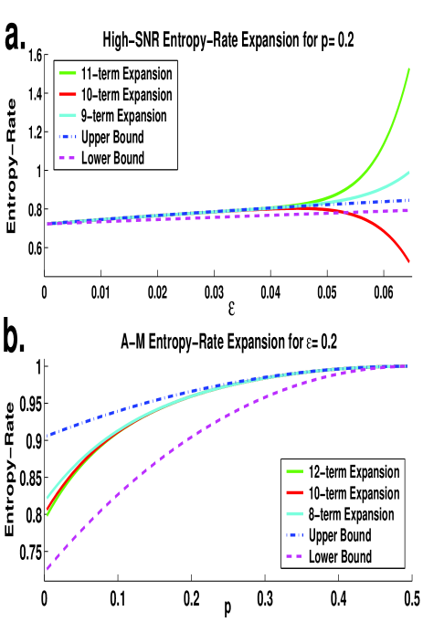
Figure 1: Approximations for $\bar{H}$ using first few terms in its series expansion. a. The High-SNR expansions using $9,10$ and $11$ terms for $p=0.2$ deviate from the bounds for large values of $\epsilon$. The first few terms of the expansion have alternating signs, therefore the direction of the deviation is determined by the parity of the number of terms taken. b. The A-M expansions using $8,10$ and $12$ terms for $\epsilon=0.2$ remain within the bounds for any value of $p$.

For the High-SNR case, we gave a numerical estimation of the radius of convergence $\rho(p)$ as a function of $p$ ([8]), based on the first few known terms. When one applies the same procedure to the coefficients of the A-M expansion, the numerical values of the estimated radius are much higher. The difference is demonstrated in fig. 1. In this figure, the (finite) series expansions with up to twelve’th order is compared to two known bounds on $\bar{H}$ from [4]. The upper bound is simply $C_{N}=H(Y_{N}|[Y]_{1}^{N-1})$ and the lower bound is $c_{N}\equiv H(Y_{N}|X_{1},[Y]_{1}^{N-1})$, for $N=2$. As can be seen from the figure, for the High-SNR case at $p=0.2$, the finite-order expansions are not within the bounds for large values of $\epsilon$. For the A-M case, for $\epsilon=0.2$, the finite-order expansions remain within the bounds for any $0<p<\frac{1}{2}$.
The estimated radius $\rho(p)$ for the High-SNR expansion, is plotted as a function of $p$ in fig. 2.a. In our context, the result of [9] proves that $\bar{H}(p,\epsilon)$ is real analytic in the domain $\Omega\subset\mathbb{R}^{2},\quad\Omega=\{(p,\epsilon):0<p,\epsilon<1\}$ (it is not known whether $\Omega$ is maximal with that respect). This domain is shown in fig. 2.b. For any $0<\epsilon<1$, the A-M expansion is near the point $(\epsilon,\frac{1}{2})$ which is an interior point of $\Omega$. The High-SNR expansion is near some point $(p,0)$, which lies on the boundary of $\Omega$.

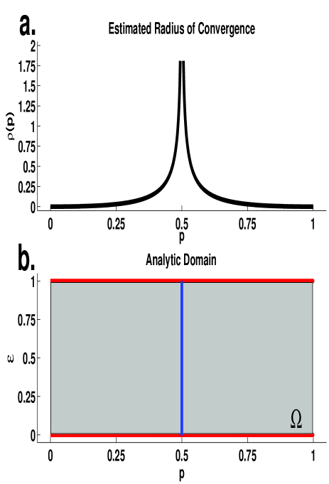
Figure 2: a. The estimated radius of convergence $\rho(p)$ for the High-SNR expansion as a function of $p$. b. The domain $\Omega$ (shaded gray area) in the $\mathbb{R}^{2}$ plane for which it is known [9] that $\bar{H}$ is real analytic in $(p,\epsilon)$. The A-M expansion is near the vertical line $p=\frac{1}{2}$. The High-SNR expansion is near the horizonal boundaries at $\epsilon=0$ and $\epsilon=1$.

V Conclusion

We presented a generalization and proof of the conjecture introduced in [7], relating the expansion coefficients of finite system entropies to those of the entropy rate for HMPs. Our new theorems shed light on the connection between finite and infinite chains, as well as give a practical and straightforward way to compute the entropy rate as a series expansion up to an arbitrary power.

The surprising ’settling’ of the expansion coefficients $C_{N}^{(k)}=C^{(k)}$ for $N\geq\lceil\frac{k+3}{2}\rceil$, hold for the entropy. For other functions involving only conditional probabilities (e.g. relative entropy between two HMPs) a weaker result holds: the coefficients ’settle’ for $N\geq k$. We note that this is still a highly non-trivial result, as it is known that for other regimes (e.g. ’rare-transitions’ [11]), a finite chain of any length does not give the correct asymptotic behavior even to the first order. We also estimated the radius of convergence for the expansion in the two regimes, ’High-SNR’ and ’A-M’, and demonstrated their quantitatively different behavior. Further research in this direction, which closely relates to the domain of analyticity of the entropy rate, is still required.

References

- [1] Y. Ephraim and N. Merhav, Hidden Markov processes, IEEE Trans. Inform. Theory, 48(6), pp. 1518-1569, June 2002.
- [2] L. R. Rabiner, A tutorial on hidden Markov models and selected applications in speech recognition, Proc. IEEE, 77(2), pp. 257-286, 1989.
- [3] C. E. Shannon, A mathematical theory of communication, Bell System Technical Journal, 27, pp. 379-423 and 623-656, 1948.
- [4] T. M. Cover and J. A. Thomas, Elements of Information Theory, Wiley, New York, 1991.
- [5] P. Jacquet, G. Seroussi and W. Szpankowski, On the Entropy of a Hidden Markov Process, DCC 2004, pp. 362-371.
- [6] E. Ordentlich and T. Weissman, New Bounds on the Entropy Rate of Hidden Markov Processes, San Antonio Information Theory Workshop, 2004.
- [7] O. Zuk, I. Kanter and E. Domany, Asymptotics of the Entropy Rate for a Hidden Markov Process, DCC 2005, pp. 173-182.
- [8] O. Zuk, I. Kanter and E. Domany, The Entropy of a Binary Hidden Markov Process, J. Stat. Phys. (in print 2005).
- [9] G. Han and B. Marcus Analyticity of Entropy Rate in Families of Hidden Markov Chains, to appear in ISIT 2005.
- [10] E. Ordentlich and T. Weissman, On the optimality of symbol-by-symbol filtering and denoising, to appear in IEEE Tra. Inf. Th.
- [11] C. Nair, E. Ordentlich and T. Weissman, On asymptotic filtering and entropy rate for a hidden Markov process in the rare transitions regime, to appear in ISIT 2005.