Tree-Based Construction of LDPC Codes Having Good Pseudocodeword Weights

Abstract

We present a tree-based construction of LDPC codes that have minimum pseudocodeword weight equal to or almost equal to the minimum distance, and perform well with iterative decoding. The construction involves enumerating a $d$-regular tree for a fixed number of layers and employing a connection algorithm based on permutations or mutually orthogonal Latin squares to close the tree. Methods are presented for degrees $d=p^{s}$ and $d=p^{s}+1$, for $p$ a prime. One class corresponds to the well-known finite-geometry and finite generalized quadrangle LDPC codes; the other codes presented are new. We also present some bounds on pseudocodeword weight for $p$-ary LDPC codes. Treating these codes as $p$-ary LDPC codes rather than binary LDPC codes improves their rates, minimum distances, and pseudocodeword weights, thereby giving a new importance to the finite geometry LDPC codes where $p>2$.

I Introduction

Low Density Parity Check (LDPC) codes are widely acknowledged to be good codes due to their near Shannon-limit performance when decoded iteratively. However, many structure-based constructions of LDPC codes fail to achieve this level of performance, and are often outperformed by random constructions. (Exceptions include the finite-geometry-based LDPC codes (FG-LDPC) of [12], which were later generalized in [19].) Moreover, there are discrepancies between iterative and maximum likelihood (ML) decoding performance of short to moderate blocklength LDPC codes. This behavior has recently been attributed to the presence of so-called pseudocodewords of the LDPC constraint graphs (or, Tanner graphs), which are valid solutions of the iterative decoder which may or may not be optimal [11]. Analogous to the role of minimum Hamming distance, $d_{\min}$, in ML-decoding, the minimum pseudocodeword weight, $w_{\min}$, has been shown to be a leading predictor of performance in iterative decoding [26]. Furthermore, the error floor performance of iterative decoding is dominated by minimum weight pseudocodewords. Although there exist pseudocodewords with weight larger than $d_{\min}$ that have adverse affects on decoding, it has been observed that pseudocodewords with weight $w_{\min}<d_{\min}$ are especially problematic [9].

Most methods for designing LDPC codes are based on random design techniques. However, the lack of structure implied by this randomness presents serious disadvantages in terms of storing and accessing a large parity check matrix, encoding data, and analyzing code performance. Therefore, by designing codes algebraically, some of these problems can be overcome. In the recent literature, several algebraic methods for constructing LDPC codes have been proposed [24][12][22][8]. These constructions are geared towards optimizing a specific parameter in the design of Tanner graphs – namely, either girth, expansion, diameter, or more recently, stopping sets. In this paper, we consider a more fundamental parameter for designing LDPC codes – namely, pseudocodewords of the corresponding Tanner graphs. While pseudocodewords are essentially stopping sets on the binary erasure channel (BEC) and have been well studied on the BEC in [5, 8, 23, 7], they have received little attention in the context of designing LDPC codes for other channels. The constructions presented in this paper are geared towards maximizing the minimum pseudocodeword weight of the corresponding LDPC Tanner graphs.

The Type I-A construction and certain cases of the Type II construction presented in this paper are designed so that the resulting codes have minimum pseudocodeword weight equal to or almost equal to the minimum distance of the code, and consequently, the problematic low-weight pseudocodewords are avoided. Some of the resulting codes have minimum distance which meets the lower tree bound originally presented in [20]. Since $w_{\min}$ shares the same lower bound [9, 10], and is upper bounded by $d_{\min}$, these constructions have $w_{\min}=d_{\min}$. It is worth noting that this property is also a characteristic of some of the FG -LDPC codes [19], and indeed, the projective-geometry-based codes of [12] arise as special cases of our Type II construction. It is worth noting, however, that the tree construction technique is simpler than that described in [12]. Furthermore, the Type I-B construction presented herein yields a family of codes with a wide range of rates and blocklengths that are comparable to those obtained from finite geometries. This new family of codes has $w_{\min}=d_{\min}\geq$ tree bound in most cases.

Both min-sum and sum-product iterative decoding performance of the tree-based constructions are comparable to, if not, better than, that of random LDPC codes of similar rates and block lengths. We now present the tree bound on $w_{\min}$ derived in [10].

Definition I.1

The tree bound of a $d$ left (variable node) regular bipartite LDPC constraint graph with girth $g$ is defined as

$$T(d,g):=\left\{\begin{array}[]{cc}1+d+d(d-1)+d(d-1)^{2}+\ldots+d(d-1)^{\frac{g-6}{4}},&\frac{g}{2}\mbox{ odd },\\ 1+d+d(d-1)+\ldots+d(d-1)^{\frac{g-8}{4}}+(d-1)^{\frac{g-4}{4}},&\frac{g}{2}\mbox{ even }.\end{array}\right.$$ (1)

Theorem I.2

Let $G$ be a bipartite LDPC constraint graph with smallest left (variable node) degree $d$ and girth $g$. Then the minimum pseudocodeword weight $w_{\min}$ (for the AWGN/BSC channels) is lower bounded by

$$\scriptsize w_{\min}\geq T(d,g).$$

This bound is also the tree bound on the minimum distance established by Tanner in [20]. And since the set of pseudocodewords includes all codewords, we have $w_{\min}\leq d_{\min}$.

We derive a pseudocodeword weight definition for the $p$-ary symmetric channel (PSC), and extend the tree lower bound on $w_{\min}$ for the PSC. The tree-based code constructions are then analyzed as $p$-ary LDPC codes. Interpreting the tree-based codes as $p$-ary LDPC codes when the degree is $d=p^{s}$ or $d=p^{s}+1$ yields codes with rates $>0.5$ and good distances. The interpretation is also meaningful for the FG LDPC codes of [12], since the projective geometry codes with $d=p^{s}+1,p>2$ have rate $\frac{1}{n}$ if treated as binary codes and rate $>0.5$ if treated as $p$-ary LDPC codes.

The paper is organized as follows. The following section introduces permutations and mutually orthogonal Latin squares. The Type I constructions are presented in Section 3 and properties of the resulting codes are discussed. Section 4 presents the Type II construction with two variations and the resulting codes are compared with codes arising from finite geometries and finite generalized quadrangles. In Section 5, we provide simulation results of the codes on the additive white Gaussian noise (AWGN) channel and on the p-ary symmetric channel. The paper is concluded in Section 6.

II Preliminaries

II-A Permutations

A permutation on set of integers modulo $m$, $\{0,1,\dots,m-1\}$ is a bijective map of the form

$$\pi:\{0,1,\dots,m-1\}\rightarrow\{0,1,\dots,m-1\}$$

A permutation is commonly denoted either as

$$\left(\begin{array}[]{ccccc}0&1&2&\dots&m-1\\ \pi(0)&\pi(1)&\pi(2)&\dots&\pi(m-1)\end{array}\right)$$

or as $(a_{11}a_{12}\dots a_{1s_{1}})(a_{21}a_{22}\dots a_{2s_{2}})\dots$, where $a_{i2}=\pi(a_{i1}),a_{i3}=\pi(a_{i2}),\dots,a_{is_{i}}=\pi(a_{i,s_{i}-1}),a_{i1}=\pi(a_{is_{i}})$ for all $i$.

As an example, suppose $\pi$ is a permutation on the set $\{0,1,2,3\}$ given by $\pi(0)=0$, $\pi(1)=2$, $\pi(2)=3$, $\pi(3)=1$. Then $\pi$ is denoted as $\left(\begin{array}[]{cccc}0&1&2&3\\ 0&2&3&1\end{array}\right)$ in the former representation, and as $(0)(123)$ in the latter representation.

II-B Mutually orthogonal Latin squares (MOLS)

Let $\mathbb{F}:=GF(q)$ be a finite field of order $q$ and let $\mathbb{F}^{*}$ denote the corresponding multiplicative group –i.e., $\mathbb{F}^{*}:=\mathbb{F}\backslash\{0\}$. For every $a\in\mathbb{F}^{*}$, we define a $q\times q$ array having entries in $\mathbb{F}$ by the following linear map

$$\phi_{a}:\mathbb{F}\times\mathbb{F}\rightarrow\mathbb{F}$$

$$(x,y)\mapsto x+a\cdot y$$

where ‘$+$’ and ‘$\cdot$’ are the corresponding field operations. The above set of maps define $q-1$ mutually orthogonal Latin squares (MOLS) [pg. 182 – 199, [21]]. The map $\phi_{a}$ can be written as a matrix $M_{a}$ where the rows and columns of the matrix are indexed by the elements of $\mathbb{F}$ and the $(x,y)^{th}$ entry of the matrix is $\phi_{a}(x,y)$. By introducing another map $\phi_{0}$ defined in the following manner

$$\phi_{0}:\mathbb{F}\times\mathbb{F}\rightarrow\mathbb{F}$$

$$(x,y)\mapsto x$$

we obtain an additional array $M_{0}$ which is orthogonal to the above family of $q-1$ MOLS. However, note that $M_{0}$ is not a Latin square. We use this set of $q$ arrays in the subsequent tree-based constructions.

As an example, let $\mathbb{F}=\{0,1,\alpha,\alpha^{2}\}$ be the finite field with four elements, where $\alpha$ represents the primitive element. Then, from the above set of maps we obtain the following four orthogonal squares

$$M_{0}:=\left[\begin{array}[]{cccc}0&0&0&0\\ 1&1&1&1\\ \alpha&\alpha&\alpha&\alpha\\ \alpha^{2}&\alpha^{2}&\alpha^{2}&\alpha^{2}\end{array}\right],\ M_{1}:=\left[\begin{array}[]{cccc}0&1&\alpha&\alpha^{2}\\ 1&0&\alpha^{2}&\alpha\\ \alpha&\alpha^{2}&0&1\\ \alpha^{2}&\alpha&1&0\end{array}\right],\ M_{\alpha}:=\left[\begin{array}[]{cccc}0&\alpha&\alpha^{2}&1\\ 1&\alpha^{2}&\alpha&0\\ \alpha&0&1&\alpha^{2}\\ \alpha^{2}&1&0&\alpha\end{array}\right],\ M_{\alpha^{2}}:=\left[\begin{array}[]{cccc}0&\alpha^{2}&1&\alpha\\ 1&\alpha&0&\alpha^{2}\\ \alpha&1&\alpha^{2}&0\\ \alpha^{2}&0&\alpha&1\end{array}\right].$$

III Tree-based Construction: Type I

In the Type I construction, first a $d$-regular tree of alternating “variable” and “constraint” node layers is enumerated downwards from a root variable node (layer $L_{0}$) for $\ell$ layers. (The variable nodes and constraint nodes in this tree are merely two different types of vertices that give rise to a bipartition in the graph.) If $\ell$ is odd (respectively, even), the final layer $L_{\ell-1}$ is composed of variable nodes (respectively, constraint nodes). Call this tree $T$. The tree $T$ is then reflected across an imaginary horizontal axis to yield another tree, $T^{\prime}$, and the variable and constraint nodes are reversed. That is, if layer $L_{i}$ in $T$ is composed of variable nodes, then the reflection of $L_{i}$, call it $L_{i}^{\prime}$, is composed of constraint nodes in the reflected tree, $T^{\prime}$. The union of these two trees, along with edges connecting the nodes in layers $L_{\ell-1}$ and $L_{\ell-1}^{\prime}$ according to a connection algorithm that is described next, comprise the graph representing a Type I LDPC code. We now present two connection schemes that can be used in this Type I model, and discuss the resulting codes.

III-A Type I-A

Figure 3 shows a 3-regular girth $10$ Type I-A LDPC constraint graph. For $d=3$, the Type I-A construction yields a $d$-regular LDPC constraint graph having $1+d+d(d-1)+\ldots+d(d-1)^{\ell-2}$ variable and constraint nodes, and girth $g$. The tree $T$ has $\ell$ layers. To connect the nodes in $L_{\ell-1}$ to $L_{\ell-1}^{\prime}$, first label the variable (resp., constraint) nodes in $L_{\ell-1}$ (resp., $L_{\ell-1}^{\prime}$) when $\ell$ is odd (and vice versa when $\ell$ is even), as $v_{0},v_{1},\dots,v_{2^{\ell-2}-1}$, $v_{2^{\ell-2}},\dots,v_{2\cdot 2^{\ell-2}-1},v_{2\cdot 2^{\ell-2}},\dots,v_{3\cdot 2^{\ell-2}-1}$ (resp., $c_{0},c_{1},\dots,c_{3\cdot 2^{\ell-2}-1}$). The nodes $v_{0},v_{1},\dots,v_{2^{\ell-2}-1}$ form the $0^{th}$ class $S_{0}$, the nodes $v_{2^{\ell-2}},\dots,v_{2\cdot 2^{\ell-2}-1}$ form the $1^{st}$ class $S_{1}$, and the nodes $v_{2\cdot 2^{\ell-2}},\dots,v_{3\cdot 2^{\ell-2}-1}$ form the $2^{nd}$ class $S_{2}$; classify the constraint nodes into $S_{0}^{\prime}$, $S_{1}^{\prime}$, and $S_{2}^{\prime}$ in a similar manner. In addition, define four permutations $\pi(\cdot),\tau(\cdot),\tau^{\prime}(\cdot),\tau^{\prime\prime}(\cdot)$ of the set $\{0,1,\dots,2^{\ell-2}-1\}$ and connect the nodes in $L_{\ell-1}$ to $L_{\ell-1}^{\prime}$ as follows: For $j=0,1,\dots,2^{\ell-2}-1$,

1. The variable node $v_{j}$ is connected to nodes $c_{\pi(j)}$ and $c_{\tau(j)+2^{\ell-2}}$.

2. The variable node $v_{j+2^{\ell-2}}$ is connected to nodes $c_{\pi(j)+2^{\ell-2}}$ and $c_{\tau^{\prime}(j)+2\cdot 2^{\ell-2}}$.

3. The variable node $v_{j+2\cdot 2^{\ell-2}}$ is connected to nodes $c_{\pi(j)+2\cdot 2^{\ell-2}}$ and $c_{\tau^{\prime\prime}(j)}$.

The permutations for the cases $g=6,8,10,12$ are given in Table I. For $\ell=3,4,5,6$, these permutations yield girths $g=6,8,10,12$, respectively, – i.e., $g=2\ell$. It is clear that the girth of these graphs is upper bounded by $2\ell$. What is interesting is that there exist permutations $\pi,\tau,\tau^{\prime},\tau^{\prime\prime}$ that achieve this upper bound when $\ell\leq 6$. However, when extending this particular construction to $\ell=7$ layers, there are no permutations $\pi,\tau,\tau^{\prime},\tau^{\prime\prime}$ that yield a girth $g=14$ graph. (This was verified by an exhaustive computer search and computing the girths of the resulting graphs using MAGMA [13].) The above algorithm to connect the nodes in layers $L_{\ell-1}$ and $L_{\ell-1}^{\prime}$ is rather restrictive, and we need to examine other connection algorithms that may possibly yield a girth 14 bipartite graph. However, the smallest known $3$-regular graph with girth $14$ has 384 vertices [1]. For $\ell=7$, the graph of the Type I-A construction has a total of 380 nodes (i.e., 190 variable nodes and 190 constraint nodes), and there are permutations $\pi,\tau,\tau^{\prime},$ and $\tau^{\prime\prime}$, that only result in a girth 12 (bipartite) graph.

Girth	$g=6$	$g=8$	$g=10$	$g=12$
$\pi$	(0)(1)	(0)(2)(1,3)	(0)(2)(4)(6)(1,5)(3,7)	(0)(4)(8)(12)(2,6)(10,14)(1,9)(3,15)(5,13)(7,11)
$\tau$	$=\pi$	$=\pi$	(0)(2)(4)(6)(1,7)(3,5)	(0)(4)(8)(12)(2,6)(10,14)(1,13)(3,11)(5,9)(7,15)
$\tau^{\prime}$	$=\pi$	$=\pi$	$=\tau$	(0,8)(4,12)(2,14)(6,10)(1,5)(3)(7)(9,13)(11)(15)
$\tau^{\prime\prime}$	$=\pi$	(0,2)(1)(3)	(0,4)(2,6)(1,3)(5,7)	(0,2,4,6)(8,10,12,14)(1,15,5,11)(3,9,7,13)

TABLE I: Permutations for Type I-A construction.

When $\ell=3,5$, the minimum distance of the resulting code meets the tree bound, and hence, $d_{\min}=w_{\min}$. When $\ell=4,6$, the minimum distance $d_{\min}$ is strictly larger than the tree bound; in fact, $d_{\min}$ is more than the tree-bound by $2$. However, $w_{\min}=d_{\min}$ for $\ell=4,6$ as well.

Remark III.1

The Type I-A LDPC codes have $d_{\min}=w_{\min}=T(d,2\ell)$, for $\ell=3,5$, and $d_{\min}=w_{\min}=2+T(d,2\ell)$, for $\ell=4,6$.

III-B Type I-B

Figure 4 provides a specific example of a Type I-B LDPC constraint graph with $d=4=2^{2}$. For $d=p^{s}$, a prime power, the Type I-B construction yields a $d$-regular LDPC constraint graph having $1+d+d(d-1)$ variable and constraint nodes, and girth at least $6$. The tree $T$ has 3 layers $L_{0},L_{1},$ and $L_{2}$. The tree is reflected to yield another tree $T^{\prime}$ and the variable and constraint nodes in $T^{\prime}$ are interchanged. Let $\alpha$ be a primitive element in the field $GF(p^{s})$. (Note that $GF(p^{s})$ is the set $\{0,1,\alpha,\alpha^{2},\dots,\alpha^{p^{s}-2}\}$.) The layer $L_{1}$ (resp., $L_{1}^{\prime}$) contains $p^{s}$ constraint nodes labeled $(0)_{c},(1)_{c},(\alpha)_{c},\dots,(\alpha^{p^{s}-2})_{c}$ (resp., variable nodes labeled $(0)^{\prime},(1)^{\prime},(\alpha)^{\prime},\dots,(\alpha^{p^{s}-2})^{\prime}$). The layer $L_{2}$ (resp., $L_{2}^{\prime}$) is composed of $p^{s}$ sets $\{S_{i}\}_{i=0,1,\alpha,\alpha^{2},\dots,\alpha^{p^{s}-2}}$ of $p^{s}-1$ variable (resp., constraint) nodes in each set. Note that we index the sets by an element of the field $GF(p^{s})$. Each set $S_{i}$ corresponds to the children of one of the branches of the root node. (The ‘^′’ in the labeling refers to nodes in the tree $T^{\prime}$ and the subscript ‘$c$’ refers to constraint nodes.) Let $S_{i}$ (resp., $S_{i}^{\prime}$) contain the variable nodes $(i,1),(i,\alpha),\ldots,(i,\alpha^{p^{s}-2})$ (resp., constraint nodes $(i,1)^{\prime}_{c},(i,\alpha)^{\prime}_{c},\ldots,(i,\alpha^{p^{s}-2})^{\prime}_{c}$). To use MOLS of order $p^{s}$ in the connection algorithm, an imaginary node, variable node $(i,0)$ (resp., constraint node $(i,0)^{\prime}_{c}$) is temporarily introduced into each set $S_{i}$ (resp, $S_{i}^{\prime}$). The connection algorithm proceeds as follows:

1. For $i=0,1,\alpha,\dots,\alpha^{p^{s}-2}$ and $j=0,1,\alpha,\dots,\alpha^{p^{s}-2}$, connect the variable node $(i,j)$ in layer $L_{2}$ to the constraint nodes

   $${\large(0,j+i\cdot 0)^{\prime}_{c},\ (1,j+i\cdot 1)^{\prime}_{c},\ \ldots,\ (\alpha^{p^{s}-2},j+i\cdot\alpha^{p^{s}-2})^{\prime}_{c}}$$

   in layer $L^{\prime}_{2}$. (Observe that in these connections, every variable node in the set $S_{i}$ is mapped to exactly one constraint node in each set $S^{\prime}_{k}$, for $k=0,1,\alpha,\dots,\alpha^{p^{s}-2}$, using the array $M_{i}$ defined in Section 2.B.)

2. Delete all imaginary nodes $\{(i,0),(i,0)^{\prime}_{c}\}_{i=0,1,\dots,\alpha^{p^{s}-2}}$ and the edges incident on them.

3. For $i=1,\ldots,\alpha^{p^{s}-2},$ delete the edge connecting variable node $(0,i)$ to constraint node $(0,i)^{\prime}_{c}$.

The resulting $d$-regular constraint graph represents the Type I-B LDPC code.

The Type I-B algorithm yields LDPC codes having a wide range of rates and blocklengths that are comparable to, but different from, the two-dimensional LDPC codes from finite Euclidean geometries [12, 19]. The Type I-B LDPC codes are $p^{s}$-regular with girth at least six, blocklength $N=p^{2s}+1$, and distance $d_{\min}\geq p^{s}+1$. For degrees of the form $d=2^{s}$, the resulting binary Type I-B LDPC codes have very good rates, above 0.5, and perform well with iterative decoding. (See Table IV.)

Theorem III.2

The Type I-B LDPC constraint graphs have a girth of at least six.

Proof:

We need to show that there are no 4-cycles in the graph. By construction, it is clear that there are no 4-cycles that involve the nodes in layers $L_{0}$, $L_{0}^{\prime}$, $L_{1}$, and $L_{1}^{\prime}$. This is because no two nodes, say, variable nodes $(i,j)$ and $(i,k)$ in a particular class $S_{i}$ are connected to the same node $(s,t)^{\prime}_{c}$ in some class $S_{s}^{\prime}$; otherwise, it would mean that $t=j+i\cdot s=k+i\cdot s$. But this is only true for $j=k$. Therefore, suppose there is a 4-cycle in the graph, then let us assume that variable nodes $(i,j)$ and $(s,t)$, for $s\neq i$, are each connected to constraint nodes $(a,b)^{\prime}_{c}$ and $(e,f)^{\prime}_{c}$. By construction, this means that $b=j+i\cdot a=t+s\cdot a$ and $f=j+i\cdot e=t+s\cdot e$. However then $j-t=(s-i)\cdot a=(s-a)\cdot e$, thereby implying that $a=e$. When $a=e$, we also have $b=j+i\cdot a=j+i\cdot e=f$. Thus, $(a,b)^{\prime}_{c}=(e,f)^{\prime}_{c}$. Therefore, there are no 4-cycles in the Type I-B LDPC graphs.
∎

Theorem III.3

The Type I-B LDPC constraint graphs with degree $d=p^{s}$ and girth $g\geq 6$ have

$$\begin{array}[]{cc}2(p^{s}-1)\geq d_{\min}\geq w_{\min}\geq T(p^{s},6)=1+p^{s}&\mbox{ for }p>2,\\ 2(p^{s})+1\geq d_{\min}\geq w_{\min}\geq T(p^{s},6)=1+p^{s}&\mbox{ for }p=2.\end{array}$$

Proof:

When $p$ is an odd prime, the assertion follows immediately. Consider the following active variable nodes to be part of a codeword: variable nodes $(0,1),(0,\alpha),\dots,(0,\alpha^{p^{s}-2})$ in $S_{0}$, and all but the first variable node in the middle layer $L_{1}^{\prime}$ of the reflected tree $T^{\prime}$: i.e., variable nodes $(1)^{\prime},(\alpha)^{\prime},(\alpha^{2})^{\prime},\dots,(\alpha^{p^{s}-2})^{\prime}$ in $L_{1}^{\prime}$. Clearly all the constraints in $L_{2}^{\prime}$ are either connected to none or exactly two of these active variable nodes. The root node in $T^{\prime}$ is connected to $p^{s}-1$ (an even number) active variable nodes and the first constraint node in $L_{1}$ of $T$ is also connected to $p^{s}-1$ active variable nodes. Hence, these $2(p^{s}-1)$ active variable nodes form a codeword. This fact along with Theorems I.2 and III.2 prove that $2(p^{s}-1)\geq d_{\min}\geq w_{\min}\geq T(p^{s},6)=1+p^{s}$.

When $p=2$, consider the following active variable nodes to be part of a codeword: the root node, variable nodes $(0,1),(0,\alpha),\dots,(0,\alpha^{p^{s}-2})$ in $S_{0}$, variable node $(\alpha^{i},\alpha^{i})$ from $S_{\alpha^{i}}$, for $i=0,1,2,\dots,p^{s}-2$, and the first two variable nodes in the middle layer of $T^{\prime}$ (i.e., variable nodes $(0)^{\prime}$,$(1)^{\prime}$). Since $p=2$, $p^{s}-1$ is odd. We need to show that all the constraints are satisfied for this choice of active variable nodes. Each constraint node in the layer $L_{1}$ of $T$ has an even number of active variable node neighbors: $(0)_{c}$ has $p^{s}$ active neighbors, and $(i)_{c}$, for $i=1,\alpha,\dots,\alpha^{p^{s}-2}$, has two, the root node and variable node $(i,i)$. It remains to check the constraint nodes in $T^{\prime}$.

In order to examine the constraints in layer $L_{2}^{\prime}$ of $T^{\prime}$, observe that the variable node $(0,\alpha^{j})$, for $j=1,2,\dots,p^{s}-2$, is connected to constraint nodes

$$(1,\alpha^{j})^{\prime}_{c},(\alpha,\alpha^{j})^{\prime}_{c},\dots,(\alpha^{p^{s}-2},\alpha^{j})^{\prime}_{c},$$

and the variable node $(\alpha^{i},\alpha^{i})$, for $i=0,1,2,\dots,p^{s}-2$, is connected to constraint nodes

$$(0,\alpha^{i})^{\prime}_{c},(1,\alpha^{i}+\alpha^{i})^{\prime}_{c},(\alpha,\alpha^{i}+\alpha^{i+1})^{\prime}_{c},\dots,(\alpha^{k},\alpha^{i+k})^{\prime}_{c},\dots,(\alpha^{p^{s}-2},\alpha^{i+p^{s}-2})^{\prime}_{c}$$

Therefore, the constraint nodes $(0,\alpha^{j})^{\prime}_{c}$, for $j=1,2,\dots,p^{s}-2$, in $S_{0}^{\prime}$ of $L_{2}^{\prime}$ are connected to exactly one active variable node from layer $L_{2}$, i.e., variable node $(\alpha^{j},\alpha^{j})$; the other active variable node neighbor is variable node $(0)^{\prime}$ in the middle layer of $T^{\prime}$. Thus, all constraints in $S_{0}^{\prime}$ are satisfied.

The constraint nodes $(1,\alpha^{j})^{\prime}_{c}$, for $j=1,2,\dots,p^{s}-2$, in $S_{1}^{\prime}$ are each connected to exactly one active variable node from $L_{2}$, i.e., variable node $(0,\alpha^{j})$ from $S_{0}$. This is because, all the remaining active variable nodes in $L_{2}$, $(\alpha^{i},\alpha^{i})$ connect to the imaginary node $(1,0)^{\prime}_{c}$ in $S_{1}^{\prime}$ (since $(1,\alpha^{i}+\alpha^{i})^{\prime}_{c}=(1,0)^{\prime}_{c}$ when the characteristic of the field $GF(p^{s})$ is $p=2$). Thus, all constraint nodes in $S_{1}^{\prime}$ have two active variable node neighbors, the other active neighbor being the variable node $(1)^{\prime}$ in the middle layer of $T^{\prime}$.

Now, let us consider the constraint nodes in $S_{\alpha^{k}}^{\prime}$, for $k=1,2,\dots,p^{s}-2$. The active variable nodes $(\alpha^{i},\alpha^{i})$, for $i=0,1,2,\dots,p^{s}-2$, are connected to the following constraint nodes

$$(\alpha^{k},1+\alpha^{k})^{\prime}_{c},(\alpha^{k},\alpha+\alpha^{k+1})^{\prime}_{c},\dots,(\alpha^{k},\alpha^{p^{s}-2}+\alpha^{p^{s}-2+k})^{\prime}_{c},$$

respectively, in class $S_{\alpha^{k}}^{\prime}$. Since $\alpha^{r}+\alpha^{k+r}\neq\alpha^{t}+\alpha^{k+t}$ for $r\neq t$, the variable nodes $(\alpha^{i},\alpha^{i})$, for $i=0,1,2,\dots,p^{s}-2$, connect to distinct nodes in $S_{\alpha^{k}}^{\prime}$. Hence, each constraint node in $S_{\alpha^{k}}^{\prime}$ has exactly two active variable node neighbors – one from $S_{0}$ and the other from the set $\{(\alpha^{i},\alpha^{i})|\ i=0,1,2,\dots,p^{s}-2\}$.

Last, we note that the root (constraint) node in $T^{\prime}$ is connected to two active variable nodes, $(0)^{\prime}$ and $(1)^{\prime}$. The total number of active variable nodes is $1+(p^{s}-1)+(p^{s}-1)+2=2p^{s}+1$. This proves that the set of $2p^{s}+1$ active variable nodes forms a codeword, thereby proving the desired bound.
∎

When $p>2$, the upper bound $2(p^{s}-1)$ on minimum distance $d_{\min}$ (and possibly also $w_{\min}$) was met among all the cases of the Type I-B construction we examined. We conjecture that in fact $d_{\min}=2(p^{s}-1)$ for the Type I-B LDPC codes of degree $d=p^{s}$ when $p>2$. Since $w_{\min}$ is lower bounded by $1+p^{s}$, we have that $w_{\min}$ is close, if not equal, to $d_{\min}$.

III-C $p$-ary LDPC codes

Let $H$ be a parity check matrix representing a $p$-ary LDPC code $\mathcal{C}$. The corresponding LDPC constraint graph $G$ that represents $H$ is an incidence graph of the parity check matrix as in the binary case. However, each edge of $G$ is now assigned a weight which is the value of the corresponding non-zero entry in $H$. (In [4, 3], LDPC codes over $GF(q)$ are considered for transmission over binary modulated channels, whereas in [18], LDPC codes over integer rings are considered for higher-order modulation signal sets.)

For convenience, we consider the special case wherein each of these edge weights are equal to one. This is the case when the parity check matrix has only zeros and ones. Furthermore, whenever the LDPC graphs have edge weights of unity for all the edges, we refer to such a graph as a binary LDPC constraint graph representing a $p$-ary LDPC code $\mathcal{C}$.

We first show that if the LDPC graph corresponding to $H$ is $d$-left (variable-node) regular, then the same tree bound of Theorem I.2 holds. That is,

Lemma III.4

If $G$ is a $d$-left regular bipartite LDPC constraint graph with girth $g$ and represents a $p$-ary LDPC code $\mathcal{C}$. Then, the minimum distance of the $p$-ary LDPC code $\mathcal{C}$ is lower bounded as

$$d_{\min}\geq T(d,g).$$

Proof:

The proof is essentially the same as in the binary case. Enumerate the graph as a tree starting at an arbitrary variable node. Furthermore, assume that a codeword in $\mathcal{C}$ contains the root node in its support. The root variable node (at layer $L_{0}$ of the tree) connects to $d$ constraint nodes in the next layer (layer $L_{1}$) of the tree. These constraint nodes are each connected to some sets of variable nodes in layer $L_{2}$, and so on. Since the graph has girth $g$, the nodes enumerated up to layer $L_{\frac{g-6}{2}}$ when $\frac{g}{2}$ is odd (respectively, $L_{\frac{g-4}{2}}$ when $\frac{g}{2}$ is even) are all distinct. Since the root node belongs to a codeword, say ${\bf c}$, it assumes a non-zero value in ${\bf c}$. Since the constraints must be satisfied at the nodes in layer $L_{1}$, at least one node in Layer $L_{2}$ for each constraint node in $L_{1}$ must assume a non-zero value in ${\bf c}$. (This is under the assumption that an edge weight times a (non-zero) value, assigned to the corresponding variable node, is not zero in the code alphabet. Since we have chosen the edge weights to be unity, such a case will not arise here. But also more generally, such cases will not arise when the alphabet and the arithmetic operations are that of a finite field. However, when working over other structures, such as finite integer rings and more general groups, such cases could arise.)

Under the above assumption, that there are at least $d$ variable nodes (i.e., at least one for each node in layer $L_{1}$) in layer $L_{2}$ that are non-zero in ${\bf c}$. Continuing this argument, it is easy to see that the number of non-zero components in ${\bf c}$ is at least $1+d+d(d-1)+\dots+d(d-1)^{\frac{g-6}{4}}$ when $\frac{g}{2}$ is odd, and $1+d+d(d-1)+\dots+d(d-1)^{\frac{g-8}{4}}+(d-1)^{\frac{g-4}{4}}$ when $\frac{g}{2}$ is even. Thus, the desired lower bound holds.
∎

We note here that in general this lower bound is not met and typically $p$-ary LDPC codes that have the above graph representation have minimum distances larger than the above lower bound.

Recall from [11, 9] that a pseudocodeword of an LDPC constraint graph $G$ is a valid codeword in some finite cover of $G$. To define a pseudocodeword for a $p$-ary LDPC code, we will restrict the discussion to LDPC constraint graphs that have edge weights of unity among all their edges – in other words, binary LDPC constraint graphs that represent $p$-ary LDPC codes. A finite cover of a graph is defined in a natural way as in [11] wherein all edges in the finite cover also have an edge weight of unity. For the rest of this section, let $G$ be a LDPC constraint graph of a $p$-ary LDPC code $\mathcal{C}$ of block length $n$, and let the weights on every edge of $G$ be unity. We define a pseudocodeword $F$ of $G$ as a $n\times p$ matrix of the form

$$F=\left[\begin{array}[]{ccccc}f_{0,0}&f_{0,1}&f_{0,2}&\dots&f_{0,p-1}\\ f_{1,0}&f_{1,1}&f_{1,2}&\dots&f_{1,p-1}\\ \vdots&\vdots&\vdots&\vdots&\vdots\\ f_{n-1,0}&f_{n-1,1}&f_{n-1,2}&\dots&f_{n-1,p-1}\end{array}\right],$$

where the pseudocodeword $F$ forms a valid codeword $\hat{\bf c}$ in a finite cover $\hat{G}$ of $G$ and $f_{i,j}$ is the fraction of variable nodes in the $i^{th}$ variable cloud, for $0\leq i\leq n-1$, of $\hat{G}$ that have the assignment (or, value) equal to $j$, for $0\leq j\leq p-1$, in $\hat{\bf c}$.

A $p$-ary symmetric channel is shown in Figure 7. The input and the output of the channel are random variables belonging to a $p$-ary alphabet that can be denoted as $\{0,1,2,\dots,p-1\}$. An error occurs with probability $\epsilon$, which is parameterized by the channel, and in the case of an error, it is equally probable for an input symbol to be altered to any one of the remaining symbols.

Following the definition of pseudoweight for the binary symmetric channel [6], we provide the following definition for the weight of a pseudocodeword on the $p$-ary symmetric channel. For a pseudocodeword $F$, let $F^{\prime}$ be the sub-matrix obtained by removing the first column in $F$. (Note that the first column in $F$ contains the entries $f_{0,0},f_{1,0},f_{2,0},\dots,f_{n-1,0}$.) Then the weight of a pseudocodeword $F$ on the $p$-ary symmetric channel is defined as follows.

Definition III.5

Let $e$ be a number such that the sum of the $e$ largest components in the matrix $F^{\prime}$, say, $f_{i_{1},j_{1}},f_{i_{2},j_{2}},\dots,f_{i_{e},j_{e}}$, exceeds $\sum_{i\neq i_{1},i_{2},\dots,i_{e}}(1-f_{i,0})$. Then the weight of $F$ on the $p$-ary symmetric channel is defined as

$$w_{PSC}(F)=\left\{\begin{array}[]{cc}2e,&\mbox{if }f_{i_{1},j_{1}}+\dots+f_{i_{e},j_{e}}=\sum_{i\neq i_{1},i_{2},\dots,i_{e}}(1-f_{i,0}),\\ 2e-1,&\mbox{if }f_{i_{1},j_{1}}+\dots+f_{i_{e},j_{e}}>\sum_{i\neq i_{1},i_{2},\dots,i_{e}}(1-f_{i,0}).\end{array}\right.\vspace{0.1in}$$

Note that in the above definition, none of the $j_{k}$’s, for $k=1,2,\dots,e$, are equal to zero, and all the $i_{k}$’s, for $k=1,2,\dots,e$, are distinct. That is, we choose at most one component in every row of $F^{\prime}$ when picking the $e$ largest components. (See the appendix for an explanation on the above definition of “weight”.)

Observe that for a codeword, the above weight definition reduces to the Hamming weight. If $F$ represents a codeword ${\bf c}$, then exactly $w=wt_{H}({\bf c})$, the Hamming weight of ${\bf c}$, rows in $F^{\prime}$ contain the entry $1$ in some column, and the remaining entries in $F^{\prime}$ are zero. Furthermore, the matrix $F$ has the entry $0$ in the first column of these $w$ rows and has the entry $1$ in the first column of the remaining rows. Therefore, from the weight definition of $F$, $e=\frac{w}{2}$ and the weight of $F$ is $2e=w$.

We define the $p$-ary minimum pseudocodeword weight of $G$ (or, minimum pseudoweight) as in the binary case, i.e., as the minimum weight of a pseudocodeword among all finite covers of $G$, and denote this as $w_{\min}(G)$ or $w_{\min}$ when it is clear that we are referring to the graph $G$.

Lemma III.6

Let $G$ be a $d$-left regular bipartite graph with girth $g$ that represents a $p$-ary LDPC code $\mathcal{C}$. Then the minimum pseudocodeword weight $w_{\min}$ on the $p$-ary symmetric channel is lower bounded as

$$w_{\min}\geq T(d,g)=\left\{\begin{array}[]{cc}(1+d+d(d-1)+d(d-1)^{2}+\ldots+d(d-1)^{\frac{g-6}{4}}),&\frac{g}{2}\mbox{ odd },\\ (1+d+d(d-1)+\ldots+d(d-1)^{\frac{g-8}{4}}+(d-1)^{\frac{g-4}{4}}),&\frac{g}{2}\mbox{ even }.\end{array}\right.$$

The proof of this result is moved to the appendix. We note that, in general, this bound is rather loose. (The inequality in (3), in the proof of Lemma III.6, is typically not tight.) Moreover, we expect that $p$-ary LDPC codes to have larger minimum pseudocodeword weights than corresponding binary LDPC codes. By corresponding binary LDPC codes, we mean the codes obtained by interpreting the given LDPC constraint graph as one representing a binary LDPC code.

III-D $p$-ary Type I-B LDPC codes

Theorem III.7

For degree $d=p^{s}$, the resulting Type I-B LDPC constraint graphs of girth $g$ that represent $p$-ary LDPC codes have minimum distance and minimum pseudocodeword weight

$$2p^{s}+1\geq d_{\min}\geq w_{\min}\geq T(d,g).$$

Proof:

Consider as active variable nodes the root node, all the variable nodes in $S_{0}$, the variable nodes $(\alpha^{i},\alpha^{i})$, for $i=0,1,2,\dots,p^{s}-2$, the first variable node $(0)^{\prime}$ in the middle layer of $T^{\prime}$ and one other variable node $(y)^{\prime}$, that we will ascertain later, in the middle layer of $T^{\prime}$.

Since the code is $p$-ary (and $p>2$), assign the value 1 to the root variable node and to all the active variable nodes in $S_{0}$. Assign the value $p-1$ to the remaining active variable nodes in $L_{2}$, (i.e., nodes $(\alpha^{i},\alpha^{i})$, $i=0,1,2,\dots,p^{s}-2$). Assign the value $1$ for the variable node $(0)^{\prime}$ in the middle layer of $T^{\prime}$ and assign the value $p-1$ for the variable node $(y)^{\prime}$ in the middle layer of $T^{\prime}$. We choose $y$ in the following manner:

The variable nodes $(\alpha^{i},\alpha^{i})$, for $i=0,1,2,\dots,p^{s}-2$, are connected to the following constraint nodes

$$(\alpha^{k},1+\alpha^{k})^{\prime}_{c},(\alpha^{k},\alpha+\alpha^{k+1})^{\prime}_{c},\dots,(\alpha^{k},\alpha^{j}+\alpha^{k+j})^{\prime}_{c},\dots,(\alpha^{k},\alpha^{p^{s}-2}+\alpha^{k+p^{s}-2})^{\prime}_{c},$$

respectively, in class $S_{\alpha^{k}}$. Either, the above set of constraint nodes are all distinct, or they are all equal to $(\alpha^{k},0)^{\prime}_{c}$. This is because, $\alpha^{r}+\alpha^{r+k}=\alpha^{t}+\alpha^{t+k}$ if and only if either, $r=t$ or $1+\alpha^{k}=0$. So there is only one $k\in\{0,1,2,\dots,p^{s}-2\}$, for which $1+\alpha^{k}=0$, and for that value of $k$, we set $y=\alpha^{k}$.

From the proof of Theorem III.3 and the above assignment, it is easily verified that each constraint node has value zero when the sum of the incoming active nodes is take modulo $p$. Thus, the set of $2p^{s}+1$ active variable nodes forms a codeword, and therefore $d_{\min}\leq 2p^{s}+1$. Hence, from Lemmas III.4 and III.6, we have $T(d,6)\leq w_{\min}\leq d_{\min}\leq 2p^{s}+1$.
∎

It is also observed that if the codes resulting from the Type I-B construction are treated as $p$-ary codes rather than binary codes when the corresponding degree in the LDPC graph is $d=p^{s}$, then the rates obtained are also $>0.5$. (See Table IV). We also believe that the minimum pseudocodeword weights (on the $p$-ary symmetric channel) are much closer to the minimum distances for these $p$-ary LDPC codes.

IV Tree-based Construction: Type II

In the Type II construction, first a $d$-regular tree $T$ of alternating variable and constraint node layers is enumerated from a root variable node (layer $L_{0}$) for $\ell$ layers $L_{0},L_{1},\dots,L_{\ell-1}$, as in Type I. The tree $T$ is not reflected; rather, a single layer of $(d-1)^{\ell-1}$ nodes is added to form layer $L_{\ell}$. If $\ell$ is odd (resp., even), this layer is composed of constraint (resp., variable) nodes. The union of $T$ and $L_{\ell}$, along with edges connecting the nodes in layers $L_{\ell-1}$ and $L_{\ell}$ according to a connection algorithm that is described next, comprise the graph representing a Type II LDPC code. We present the connection scheme that is used for this Type II model, and discuss the resulting codes. First, we state this rather simple observation without proof:

The girth $g$ of a Type II LDPC graph for $\ell$ layers is at most $2\ell$.

The connection algorithm for $\ell=3$ and $\ell=4$, wherein this upper bound on girth is in fact achieved, is as follows.

IV-A $\ell=3$

Figure 5 provides an example of a Type II LDPC constraint graph for $\ell=3$ layers, with degree $d=4=3+1$ and girth $g=6$. For $d=p^{s}+1$, where $p$ is prime and $s$ a positive integer, a $d$-regular tree is enumerated from a root (variable) node for $\ell=3$ layers $L_{0},L_{1},L_{2}$. Let $\alpha$ be a primitive element in the field $GF(p^{s})$. The $d$ constraint nodes in $L_{1}$ are labeled $(x)_{c},(0)_{c},(1)_{c},(\alpha)_{c},\dots,(\alpha^{p^{s}-2})_{c}$ to represent the $d$ branches stemming from the root node. Note that the first constraint node is denoted as $(x)_{c}$ and the remaining constraint nodes are indexed by the elements of the field $GF(p^{s})$. The $d(d-1)$ variable nodes in the third layer $L_{2}$ are labeled as follows: the variable nodes descending from constraint node $(x)_{c}$ form the class $S_{x}$ and are labeled $(x,0),(x,1),\dots,(x,\alpha^{p^{s}-2})$, and the variable nodes descending from constraint node $(i)_{c}$, for $i=0,1,\alpha,\dots,\alpha^{p^{s}-2}$, form the class $S_{i}$ and are labeled $(i,0),(i,1),\dots,(i,\alpha^{p^{s}-2})$.

A final layer $L_{\ell}=L_{3}$ of $(d-1)^{\ell-1}=p^{2s}$ constraint nodes is added. The $p^{2s}$ constraint nodes in $L_{3}$ are labeled $(0,0)^{\prime}_{c},(0,1)^{\prime}_{c},\dots,(0,\alpha^{p^{s}-2})^{\prime}_{c}$, $(1,0)^{\prime}_{c}$, $(1,1)^{\prime}_{c}$, $\dots$, $(1,\alpha^{p^{s}-2})^{\prime}_{c}$, $\dots$, $(\alpha^{p^{s}-2},0)^{\prime}_{c}$, $(\alpha^{p^{s}-2},1)^{\prime}_{c}$, $\dots$, $(\alpha^{p^{s}-2},\alpha^{p^{s}-2})^{\prime}_{c}$. (Note that the ‘^′’ in the labeling refers to nodes in that are not in the tree $T$ and the subscript ‘$c$’ refers to constraint nodes.)

1. By this labeling, the constraint nodes in $L_{3}$ are grouped into $d-1=p^{s}$ classes of $d-1=p^{s}$ nodes in each class. Similarly, the variable nodes in $L_{2}$ are grouped into $d=p^{s}+1$ classes of $d-1=p^{s}$ nodes in each class. (That is, the $i^{th}$ class of constraint nodes is $S_{i}^{\prime}=\{(i,0)^{\prime}_{c},(i,1)^{\prime}_{c},\dots,(i,\alpha^{p^{s}-2})^{\prime}_{c}\}$.)

2. The variable nodes descending from constraint node $(x)_{c}$ are connected to the constraint nodes in $L_{3}$ as follows. Connect the variable node $(x,i)$, for $i=0,1,\dots,\alpha^{p^{s}-2}$, to the constraint nodes

   $$(i,0)^{\prime}_{c},\ (i,1)^{\prime}_{c},\ \dots,\ (i,\alpha^{p^{s}-2})^{\prime}_{c}.$$

3. The remaining variable nodes in layer $L_{2}$ are connected to the nodes in $L_{3}$ as follows: Connect the variable node $(i,j)$, for $i=0,1,\alpha,\dots,\alpha^{p^{s}-2}$, $j=0,1,\dots,\alpha^{p^{s}-2}$, to the constraint nodes

   $$(0,j+i\cdot 0)^{\prime}_{c},\ (1,j+i\cdot 1)^{\prime}_{c},\ (\alpha,j+i\cdot\alpha)^{\prime}_{c},\ \dots,\ (\alpha^{p^{s}-2},j+i\cdot\alpha^{p^{s}-2})^{\prime}_{c}.$$

   Observe that in these connections, each variable node $(i,j)$ is connected to exactly one constraint node within each class, using the array $M_{i}$ defined in Section 2.B.
   

In the example illustrated in Figure 5, the arrays used for constructing the Type II LDPC constraint graph are

$$\tiny M_{0}=\left[\begin{array}[]{ccc}0&0&0\\ 1&1&1\\ 2&2&2\end{array}\right],\ M_{1}=\left[\begin{array}[]{ccc}0&1&2\\ 1&2&0\\ 2&0&1\end{array}\right],\ M_{2}=\left[\begin{array}[]{ccc}0&2&1\\ 1&0&2\\ 2&1&0\end{array}\right].$$

The ratio of minimum distance to blocklength of the resulting codes is at least $\frac{2+p^{s}}{1+p^{s}+p^{2s}}$, and the girth is six. For degrees $d$ of the form $d=2^{s}+1$, the tree bound of Theorem I.2 on minimum distance and minimum pseudocodeword weight [20, 10] is met, i.e., $d_{\min}=w_{\min}=2+2^{s}$, for the Type II, $\ell=3$, LDPC codes. For $p>2$, the resulting binary LDPC codes are repetition codes of the form $[n,1,n]$, i.e., $d_{\min}=n=1+p^{s}+p^{2s}$ and the rate is $\frac{1}{n}$. However, if we interpret the Type II $\ell=3$ graphs, that have degree $d=p^{s}+1$, as the LDPC constraint graph of a $p$-ary LDPC code, then the rates of the resulting codes are very good and the minimum distances come close to (but are not equal to) the tree bound in Lemma III.4. (See also [17].) In summary, we state the following results:

• The rate of a p-ary Type II, $\ell=3$ LDPC code is $\frac{p^{2s}+p^{s}-\frac{p^{s}(p+1)^{s}}{2^{s}}}{p^{2s}+p^{s}+1}$ [14].

• The rate of a binary Type II, $\ell=3$ LDPC code is $\frac{1}{n}$ for $p>2$.

Note that binary codes with $p=2$ are a special case of $p$-ary LDPC codes. Moreover, the rate expression for $p$-ary LDPC codes is meaningful for a wide variety of $p$’s and $s$’s. The rate expression for binary codes with $p>2$ can be seen by observing that any $t$ rows of the corresponding parity-check matrix $H$ is linearly independent if $t<n$. Since the parity-check matrix is equivalent to one obtainable from cyclic difference sets, this can be proven by showing that for any $t<n$, there exists a set of $t$ consecutive positions in the first row of $H$ that has an odd number of ones.

IV-B Relation to finite geometry codes

The codes that result from this $\ell=3$ construction correspond to the two-dimensional projective-geometry-based LDPC (PG LDPC) codes of [19]. We state the equivalence of the tree construction and the finite projective geometry based LDPC codes in the following.

Theorem IV.1

The LDPC constraint graph obtained from the Type II $\ell=3$ tree construction for degree $d=p^{s}+1$ is equivalent to the incidence graph of the finite projective plane over the field $GF(p^{s})$.

It has been proved by Bose [2] that a finite projective plane (in other words, a two dimensional finite projective geometry) of order $m$ exists if and only if a complete family of orthogonal $m\times m$ Latin squares exists. The proof of this result, as presented in [16], gives a constructive algorithm to design a finite projective plane of order $m$ from a complete family of $m\times m$ mutually orthogonal Latin squares (MOLS). It is well known that a complete family of mutually orthogonal Latin squares exists when $m=p^{s}$, a power of a prime, and we have described one such family in Section 2. Hence, the constructive algorithm in [16] generates the incidence graph of the projective plane $PG(2,p^{s})$ from the set of $p^{s}-1$ MOLS of order $p^{s}$. The only remaining step is to verify that the incidence matrix of points over lines of this projective plane is the same as the parity check matrix of variable nodes over constraint nodes of the tree-based LDPC constraint graph of the tree construction. This step is easy to verify as the constructive algorithm in [16] is analogous to the tree construction presented in this paper.

The Type II $\ell=3$ graphs therefore correspond to the two-dimensional projective-geometry-based LDPC codes of [12]. With a little modification of the Type II construction, we can also obtain the two-dimensional Euclidean-geometry-based LDPC codes of [12, 19]. Since a two-dimensional Euclidean geometry may be obtained by deleting certain points and line(s) of a two-dimensional projective geometry, the graph of a two-dimensional EG-LDPC code [19] may be obtained by performing the following operations on the Type II, $\ell=3$, graph:

1. In the tree $T$, the root node along with its neighbors, i.e., the constraint nodes in layer $L_{1}$, are deleted.

2. Consequently, the edges from the constraint nodes $(x)_{c},(0)_{c},(1)_{c},\ldots,(\alpha^{p^{s}-2})_{c}$ to layer $L_{2}$ are also deleted.

3. At this stage, the remaining variable nodes have degree $p^{s}$, and the remaining constraint nodes have degree $p^{s}+1$. Now, a constraint node from layer $L_{3}$ is chosen, say, constraint node $(0,0)^{\prime}_{c}$. This node and its neighboring variable nodes and the edges incident on them are deleted. Doing so removes exactly one variable node from each class of $L_{2}$, and the degrees of the remaining constraint nodes in $L_{3}$ are lessened by one. Thus, the resulting graph is now $p^{s}$-regular with a girth of six, has $p^{2s}-1$ constraint and variable nodes, and corresponds to the two-dimensional Euclidean-geometry-based LDPC code $EG(2,p^{s})$ of [19].
   

Theorem IV.2

The Type II $\ell=3$ LDPC constraint graphs have girth $g=6$ and diameter $\delta=3$.

Proof:

We need to show is that there are no 4-cycles in the graph. As in the proof of Theorem III.2, by construction, there are no 4-cycles that involve the nodes in layers $L_{0}$ and $L_{1}$. This is because, first, no two variable nodes in the first class $S_{x}=\{(x,0),(x,1),\dots,(x,\alpha^{p^{s}-2})\}$ are connected to the same constraint node. Next, if two variable nodes, say, $(i,j)$ and $(i,k)$ in the $i^{th}$ class $S_{i}$, for some $i\neq x$, are connected to a constraint node $(s,t)^{\prime}_{c}$, then it would mean that $t=j+i\cdot s=k+i\cdot s$. But this is only true for $j=k$. Hence, there is no 4-cycle of the form $(i)_{c}\rightarrow(i,j)\rightarrow(s,t)^{\prime}_{c}\rightarrow(i,k)\rightarrow(i)$. Therefore, suppose there is a 4-cycle in the graph, then let us consider two cases as follows. Case 1) Assume that variable nodes $(i,j)$ and $(s,t)$, for $i\neq s$ and $i\neq x\neq s$, are each connected to constraint nodes $(a,b)^{\prime}_{c}$ and $(e,f)^{\prime}_{c}$. By construction, this means that $b=j+i\cdot a=t+s\cdot a$ and $f=j+i\cdot e=t+s\cdot e$. This implies that $j-t=(s-i)\cdot a=(s-i)\cdot e$, thereby implying that $a=e$. Consequently, we also have $b=j+i\cdot a=j+i\cdot e=f$. Thus, $(a,b)^{\prime}_{c}=(e,f)^{\prime}_{c}$. Case 2) Assume that two variable nodes, one in $S_{x}$, say, $(x,j)$, and the other in $S_{i}$, (for $i\neq x$), say, $(i,k)$, are connected to constraint nodes $(a,b)^{\prime}_{c}$ and $(e,f)^{\prime}_{c}$. Then this would mean that $a=e=j$. But since $(i,k)$ connects to exactly one constraint node whose first index is $j$, this case is not possible. Thus, there are no 4-cycles in the Type II-$\ell=3$ LDPC graphs.

To show that the girth is exactly six, we see that the following nodes form a six-cycle in the graph: the root-node, the first two constraint nodes $(x)_{c}$ and $(1)_{c}$ in layer $L_{1}$, variable nodes $(x,0)$ and $(0,0)$ in layer $L_{2}$, and the constraint node $(0,0)^{\prime}_{c}$ in layer $L_{3}$.

To prove the diameter, we first observe that the root node is at distance of at most three from any other node. Similarly, it is also clear that the nodes in layer $L_{1}$ are at a distance of at most three from any other node. Therefore, it is only necessary to show that any two nodes in layer $L_{2}$ are at most distance two apart and similarly show that any two nodes in $L_{3}$ are at most distance two apart. Consider two nodes $(i,j)$ and $(s,t)$ in $L_{2}$. If $s=i$, then clearly, there is a path of length two via the parent node $(i)_{c}$. If $s\neq i$ and $s\neq x\neq i$, then by the property of a complete family of orthogonal Latin squares there is a node $(a,b)^{\prime}_{c}$ in $L_{3}$ such that $b=j+i\cdot a=t+s\cdot a$. This implies that $(i,j)$ and $(s,t)$ are connected by a distance two path via $(a,b)^{\prime}_{c}$. We can similarly show that if $s\neq i$ and $i=x$, then the node $(j,t+s\cdot j)^{\prime}_{c}$ in $L_{3}$ connects to both $(x,j)$ and $(s,t)$. A similar argument shows that any two nodes in $L_{3}$ are distance two apart. This completes the proof.
∎

Theorem IV.3

For degrees $d=2^{s}+1$, the resulting Type II $\ell=3$ LDPC constraint graphs have

$$d_{\min}=w_{\min}=T(d,6)=2+2^{s}.$$

For degrees $d=p^{s}+1$, $p>2$, when the resulting Type II $\ell=3$ LDPC constraint graphs represent $p$-ary linear codes, the corresponding minimum distance and minimum pseudocodeword weight satisfy

$$T(p^{s}+1,6)\leq w_{\min}\leq d_{\min}\leq 2p^{s}.$$

Proof:

Let us first consider the case $p=2$. We will show that the following set of active variable nodes in the Type II $\ell=3$ LDPC constraint graph form a minimum-weight codeword: the root (variable) node, variable nodes $(x,0)$, $(0,0)$, $(1,\alpha^{p^{s}-2})$, $(\alpha,\alpha^{p^{s}-3})$, $(\alpha^{2},\alpha^{p^{s}-4})$, $\dots$, $(\alpha^{i},\alpha^{p^{s}-2-i})$, $\dots$, $(\alpha^{p^{s}-2},1)$ in layer $L_{2}$.

It is clear from this choice that there is exactly one active variable node from each class in layer $L_{2}$. Therefore, all the constraint nodes at layer $L_{1}$ are satisfied. The constraint nodes in the first class $S_{0}^{\prime}$ of $L_{3}$ are $(0,0)^{\prime}_{c},(0,1)^{\prime}_{c},\dots,(0,\alpha^{p^{s}-2})^{\prime}_{c}$. The constraint node $(0,0)^{\prime}_{c}$ is connected to $(x,0)$ and $(0,0)$, and the constraint node $(0,\alpha^{i})^{\prime}_{c}$, for $i=0,1,2,\dots,p^{s}-2$, is connected to variable nodes $(x,0)$ and $(\alpha^{i},\alpha^{p^{s}-2-i})$. Thus, all constraint nodes in $S_{0}^{\prime}$ are satisfied. Let us consider the constraint nodes in class $S_{\alpha^{i}}^{\prime}$, for $i\in\{0,1,2,\dots,p^{s}-2\}$. The variable node $(0,0)$ connects to the constraint node $(\alpha^{i},0)^{\prime}_{c}$ in $S_{\alpha^{i}}^{\prime}$. The variable node $(1,\alpha^{p^{s}-2})$ connects to the constraint node $(\alpha^{i},\alpha^{p^{s}-2}+\alpha^{i})^{\prime}_{c}$ in $S_{\alpha^{i}}^{\prime}$, and in general, for $j=0,1,2,\dots,p^{s}-2$, the variable node $(\alpha^{j},\alpha^{p^{s}-2-j})$ connects to the constraint node $(\alpha^{i},\alpha^{p^{s}-2-j}+\alpha^{i+j})^{\prime}_{c}$ in $S_{\alpha^{i}}^{\prime}$. So enumerating all the constraint nodes in $S_{\alpha^{i}}^{\prime}$, with multiplicities, that are connected to an active variable node in $L_{2}$, we obtain
$(\alpha^{i},0)^{\prime}_{c}$, $(\alpha^{i},\alpha^{p^{s}-2}+\alpha^{i})^{\prime}_{c}$, $(\alpha^{i},\alpha^{p^{s}-3}+\alpha^{i+1})^{\prime}_{c}$, $\dots$, $(\alpha^{i},\alpha^{p^{s}-(p^{s}-i-1)}+\alpha^{p^{s}-3})^{\prime}_{c}$, $(\alpha^{i},\alpha^{p^{s}-(p^{s}-i)}+\alpha^{p^{s}-2})^{\prime}_{c}$, $\dots$.

Simplifying the exponents and rewriting this list, we see that, when $i$ is odd, the constraint nodes are

$(\alpha^{i},0)^{\prime}_{c}$, $(\alpha^{i},\alpha^{p^{s}-2}+\alpha^{i})^{\prime}_{c}$, $(\alpha^{i},\alpha^{p^{s}-3}+\alpha^{i+1})^{\prime}_{c}$, $\dots$, $(\alpha^{i},\alpha^{i+1}+\alpha^{p^{s}-3})^{\prime}_{c}$, $(\alpha^{i},\alpha^{i}+\alpha^{p^{s}-2})^{\prime}_{c}$, $(\alpha^{i},\alpha^{i-1}+1)^{\prime}_{c}$, $(\alpha^{i},\alpha^{i-2}+\alpha)^{\prime}_{c}$, $\dots$, $(\alpha^{i},\alpha^{(i-1)/2}+\alpha^{(i-1)/2})^{\prime}_{c}$,$\dots$, $(\alpha^{i},\alpha+\alpha^{i-2})^{\prime}_{c}$, $(\alpha^{i},1+\alpha^{i-1})^{\prime}_{c}$.

(When $i$ is even, the constraint nodes are $(\alpha^{i},0)^{\prime}_{c}$, $(\alpha^{i},\alpha^{p^{s}-2}+\alpha^{i})^{\prime}_{c}$, $(\alpha^{i},\alpha^{p^{s}-3}+\alpha^{i+1})^{\prime}_{c}$, $\dots$, $(\alpha^{i},\alpha^{(p^{s}-2+i)/2}+\alpha^{(p^{s}-2+i)/2})^{\prime}_{c}$, $\dots$, $(\alpha^{i},\alpha^{i+1}+\alpha^{p^{s}-3})^{\prime}_{c}$, $(\alpha^{i},\alpha^{i}+\alpha^{p^{s}-2})^{\prime}_{c}$, $(\alpha^{i},\alpha^{i-1}+1)^{\prime}_{c}$, $(\alpha^{i},\alpha^{i-2}+\alpha)^{\prime}_{c}$, $\dots$, $(\alpha^{i},\alpha^{i}+\alpha^{i-1})^{\prime}_{c}$, $(\alpha^{i},\alpha^{i-1}+\alpha^{i})^{\prime}_{c}$,$\dots$, $(\alpha^{i},1+\alpha^{i-1})^{\prime}_{c}$.) (Note that for $\beta\in GF(p^{s})$, $\beta+\beta=0$ when the characteristic of the field $GF(p^{s})$ is two (i.e., $p=2$).)

Observe that each of the constraint nodes in the above list appears exactly twice. Therefore, each constraint node in the list is connected to two active variable nodes in $L_{2}$, and hence, all the constraints in $S_{\alpha^{i}}^{\prime}$ are satisfied. So we have that the set of $1+2^{s}+1$ active variable nodes forms a codeword. Furthermore, they must form a minimum-weight codeword since $d_{\min}\geq 2+2^{s}=T(2^{s}+1,6)$ by the tree bound of Theorem I.2. This also proves that $d_{\min}=w_{\min}=T(d,6)$ for $d=2^{s}+1$.

Now let us consider the case $p>2$. The resulting codes are treated as $p$-ary codes. Consider the following set of active variable nodes: the root node, all but one of the nodes $(x,y)$, for an appropriately chosen $y$, in class $S_{x}$, and the nodes $(\alpha^{i},\alpha^{i})$, for $i=0,1,2,\dots,p^{s}-2$. We have chosen $2p^{s}$ active variable nodes in all.

The variable nodes $(1,1),(\alpha,\alpha),\dots,(\alpha^{p^{s}-2},\alpha^{p^{s}-2})$ are connected to constraint nodes

$$(\alpha^{k},0)^{\prime}_{c},(\alpha^{k},1+\alpha^{k})^{\prime}_{c},(\alpha^{k},\alpha+\alpha^{k+1})^{\prime}_{c},\dots,(\alpha^{k},\alpha^{j}+\alpha^{k+j})^{\prime}_{c},\dots,(\alpha^{k},\alpha^{i}+\alpha^{k+p^{s}-2})^{\prime}_{c},$$

respectively, in class $S_{\alpha^{k}}^{\prime}$ of constraint nodes in layer $L_{3}$. These nodes are either all distinct or all equal to $(\alpha^{k},0)^{\prime}_{c}$ since $\alpha^{r}+\alpha^{k+r}=\alpha^{t}+\alpha^{k+t}$ if and only if either $r=t$ or $1+\alpha^{k}=0$. Since $1+\alpha^{k}$ is zero for exactly one value of $k\in\{0,1,2,\dots,p^{s}-2\}$, we have that the variable nodes $(\alpha^{i},\alpha^{i})$, for $i=0,1,2,\dots,p^{s}-2$, are connected to distinct constraint nodes in all but one class $S_{\alpha^{k*}}$ and that, in $S_{\alpha^{k*}}$, they are all connected to the constraint node $(\alpha^{k*},0)^{\prime}_{c}$. (Note that $k*$ satisfies $1+\alpha^{k*}=0$.) We let $y=\alpha^{k*}$. Therefore, the set of active variable nodes includes all nodes of the form $(x,t)$, for $t=0,1,\alpha,\alpha^{2},\dots$, excluding node $(x,y)$.

Since the code is $p$-ary, assign the following values to the chosen set of active variable nodes: assign the value 1 to the root variable node and to all the active variable nodes in class $S_{x}$, and assign the value $p-1$ to the active variable nodes $(\alpha^{i},\alpha^{i})$, for $i=0,1,2,\dots,p^{s}-2$. It is now easy to verify that all the constraints are satisfied. Thus, $d_{\min}\leq 2p^{s}$. From Theorem IV.2 and Lemmas III.4 and III.6, we have $T(p^{s}+1,6)\leq w_{\min}\leq d_{\min}\leq 2p^{s}$.
∎

For degrees $d=p^{s}+1$, $p>2$, treating the Type II $\ell=3$ LDPC constraint graphs as binary LDPC codes, yields $[n,1,n]$ repetition codes, where $n=p^{2s}+p^{s}+1$, $d_{\min}=n$, and dimension is $1$. However, when the Type II $\ell=3$ LDPC constraint graphs, for degrees $d=p^{s}+1$, $p>2$, are treated as $p$-ary LDPC codes, we believe that the distance $d_{\min}\geq p^{s}+3$, and that this bound is in fact tight. We also suspect that the minimum pseudocodeword weights (on the $p$-ary symmetric channel) are much closer to the minimum distances for these $p$-ary LDPC codes.

IV-C $\ell=4$

Figure 6 provides an example of a Type II $\ell=4$ LDPC constraint graph with degree $d=2+1=3$ and girth $g=8$. For $d=p^{s}+1$, $p$ a prime and $s$ a positive integer, a $d$ regular tree $T$ is enumerated from a root (variable) node for $\ell=4$ layers $L_{0},L_{1},L_{2},L_{3}$.

1. The nodes in $L_{0},L_{1},$ and $L_{2}$ labeled as in the $\ell=3$ case. The constraint nodes in $L_{3}$ are labeled as follows: The constraint nodes descending from variable node $(x,j)$, for $j=0,1,,\alpha,\dots,\alpha^{p^{s}-2}$, are labeled $(x,j,0)_{c},(x,j,1)_{c},\dots,(x,j,\alpha^{p^{s}-2})_{c}$, the constraint nodes descending from variable node $(i,j)$, for $i,j=0,1,,\alpha,\dots,\alpha^{p^{s}-2}$, are labeled $(i,j,0)_{c},(i,j,1)_{c},\dots,(i,j,\alpha^{p^{s}-2})_{c}$.

2. A final layer $L_{\ell}=L_{4}$ of $(d-1)^{\ell-1}=p^{3s}$ variable nodes is introduced. The $p^{3s}$ variable nodes in $L_{4}$ are labeled as $(0,0,0)^{\prime},(0,0,1)^{\prime},\dots,(0,0,\alpha^{p^{s}-2})^{\prime}$, $(0,1,0)^{\prime},(0,1,1)^{\prime},\dots,(0,1,\alpha^{p^{s}-2})^{\prime}$, $\dots$, $(\alpha^{p^{s}-2},0,0)^{\prime},$ $(\alpha^{p^{s}-2},0,1)^{\prime},$ $\dots,$ $(\alpha^{p^{s}-2},0,\alpha^{p^{s}-2})^{\prime}$, $\dots,$ $(\alpha^{p^{s}-2},\alpha^{p^{s}-2},0)^{\prime}$, $(\alpha^{p^{s}-2},\alpha^{p^{s}-2},1)^{\prime},$ $\dots,$ $(\alpha^{p^{s}-2},\alpha^{p^{s}-2},\alpha^{p^{s}-2})^{\prime}$. (Note that the ‘^′’ in the labeling refers to nodes that are not in the tree $T$ and the subscript ‘$c$’ refers to constraint nodes.)

3. For $0\leq i\leq p^{s}-1$, $0\leq j\leq p^{s}-1$, connect the constraint node $(x,i,j)_{c}$ to the variable nodes

   $$(i,j,0)^{\prime},(i,j,1)^{\prime},(i,j,\alpha)^{\prime},\dots,(i,j,\alpha^{p^{s}-2})^{\prime}.$$

4. To connect the remaining constraint nodes in $L_{3}$ to the variable nodes in $L_{4}$, we first define a function $f$. For $i,j,k,t=0,1,\alpha,\dots,\alpha^{p^{s}-2}$ let

   $$f:\mathbb{F}\times\mathbb{F}\times\mathbb{F}\times\mathbb{F}\rightarrow\mathbb{F}$$

   $$(i,j,k,t)\mapsto y,$$

   be an appropriately chosen function, that we will define later for some specific cases of the Type II $\ell=4$ construction. Then, for $i,j,k=0,1,\alpha,\dots,\alpha^{p^{s}-2}$ , connect the constraint node $(i,j,k)_{c}$ in $L_{3}$ to the following variable nodes in $L_{4}$

   $$(0,k+i\cdot 0,f(i,j,k,0))^{\prime},\ (1,k+i\cdot 1,f(i,j,k,1))^{\prime},\ (\alpha,k+i\cdot\alpha,f(i,j,k,\alpha))^{\prime},\ ..,\ (\alpha^{p^{s}-2},k+i\cdot\alpha^{p^{s}-2},f(i,j,k,\alpha^{p^{s}-2}))^{\prime}.$$

   (Observe that the second index corresponds to the linear map defined by the array $M_{i}$ defined in Section 2.B. Further, note that if $f(i,j,k,t)=j+i\cdot t$, then the resulting graphs obtained from the above set of connections have girth at least six. However, there are other functions $f(i,j,k,t)$ for which the resulting graphs have girth exactly eight, which is the best possible when $\ell=4$ in this construction. At this point, we do not have a closed form expression for the function $f$ and we only provide details for specific cases below. (These cases were verified using the MAGMA software [13].)
   

The Type II, $\ell=4$, LDPC codes have girth eight, minimum distance $d_{\min}\geq 2(p^{s}+1)$, and blocklength $N=1+p^{s}+p^{2s}+p^{3s}$. (We believe that the tree bound on the minimum distance is met for most of the Type II, $\ell=4$, codes, i.e. $d_{\min}=w_{\min}=2(p^{s}+1)$.) For $d=3$, the Type II, $\ell=4$, LDPC constraint graph as shown in Figure 6 corresponds to the $(2,2)$-Finite-Generalized-Quadrangles-based LDPC (FGQ LDPC) code of [25]; the function $f$ used in constructing this example is defined by $f(i,j,k,t)=j+(i+1)\cdot t$, i.e., the map defined by the array $M_{i+1}$. The orthogonal arrays used for constructing this code are

$$\tiny M_{0}=\left[\begin{array}[]{cc}0&0\\ 1&1\end{array}\right],\ M_{1}=\left[\begin{array}[]{cc}0&1\\ 1&0\end{array}\right].$$

We now state some results concerning the choice of the function $f$.

1. The Type II $\ell=4$ construction results in incidence graphs of finite generalized quadrangles for appropriately chosen functions $f$. These graphs have girth $8$ and diameter $4$.

2. For some specific cases, examples of the function $f(i,j,k,t)$ that resulted in a girth $8$ graph is given in Table II. (Note that for the second entry in the table, the function $g:GF(4)\rightarrow GF(4)$ is defined by the following maps: $0\mapsto 1$, $1\mapsto\alpha$, $\alpha\mapsto\alpha^{2}$, and $\alpha^{2}\mapsto 0$.) We have not been able to find a general relation or a closed form expression for $f$ yet.

   $p$	$s$	elements	degree	$f(i,j,k,t)$
   		of $GF(p^{s})$	$d=p^{s}+1$
   2	1	$\{0,1\}$	3	$j+(i+1)\cdot t$
   2	2	$\{0,1,\alpha,\alpha^{2}\}$	5	$j+g(i)\cdot t$
   3	1	$\{0,1,2\}$	4	$i\cdot(k+2\cdot i\cdot t)+j$
   3	2	$\{0,1,\alpha,..,\alpha^{7}\}$	10	$i\cdot(k+\alpha\cdot i\cdot t)+j$
   5	1	$\{0,1,2,3,4\}$	6	$i\cdot(k+3\cdot i\cdot t)+j$
   7	1	$\{0,1,2,..,6\}$	8	$i\cdot(k+4\cdot i\cdot t)+j$

   TABLE II: The function $f$ for the Type II $\ell=4$ construction.

3. For the above set of functions, the resulting Type II $\ell=4$ LDPC constraint graphs have minimum distance meeting the tree bound, when $p=2$, i.e., $d_{\min}=w_{\min}=2(2^{s}+1)$. We conjecture that, in general, for degrees $d=2^{s}+1$, the Type II $\ell=4$ girth eight LDPC constraint graphs have $d_{\min}=w_{\min}=T(2^{s}+1,8)=2(2^{s}+1)$.

4. For degrees $d=p^{s}+1$, $p>2$, we expect the corresponding $p$-ary LDPC codes from this construction to have minimum distances $d_{\min}$ either equal or very close to the tree bound. Hence, we also expect the corresponding minimum pseudocodeword weight $w_{\min}$ to be close to $d_{\min}$.

The above results were verified using MAGMA and computer simulations.

IV-D Remarks

It is well known in the literature that finite generalized polygons (or, $N$-gons) of order $p^{s}$ exist [15]. A finite generalized $N$-gon is a non-empty point-line geometry, and consists of a set $\mathcal{P}$ of points and a set $\mathcal{L}$ of lines such that the incidence graph of this geometry is a bipartite graph of diameter $N$ and girth $2N$. Moreover, when each point is incident on $t+1$ lines and each line contains $t+1$ points, the order of the $N$-gon is said be to $t$. The Type II $\ell=3$ and $\ell=4$ constructions yield finite generalized $3$-gons and $4$-gons, respectively, of order $p^{s}$. These are essentially finite projective planes and finite generalized quadrangles. The Type II construction can be similarly extended to larger $\ell$. We believe that finding the right connections for connecting the nodes between the last layer in $T$ and the final layer will yield incidence graphs of these other finite generalized polygons. For instance, for $\ell=6$ and $\ell=8$, the construction can yield finite generalized hexagons and finite generalized octagons, respectively. We conjecture that the incidence graphs of generalized $N$-gons yield LDPC codes with minimum pseudocodeword weight $w_{\min}$ very close to the corresponding minimum distance $d_{\min}$ and particularly, for generalized $N$-gons of order $2^{s}$, the LDPC codes have $d_{\min}=w_{\min}=T(2^{s}+1,2N)$.

V Simulation Results

V-A Performance with min-sum iterative decoding

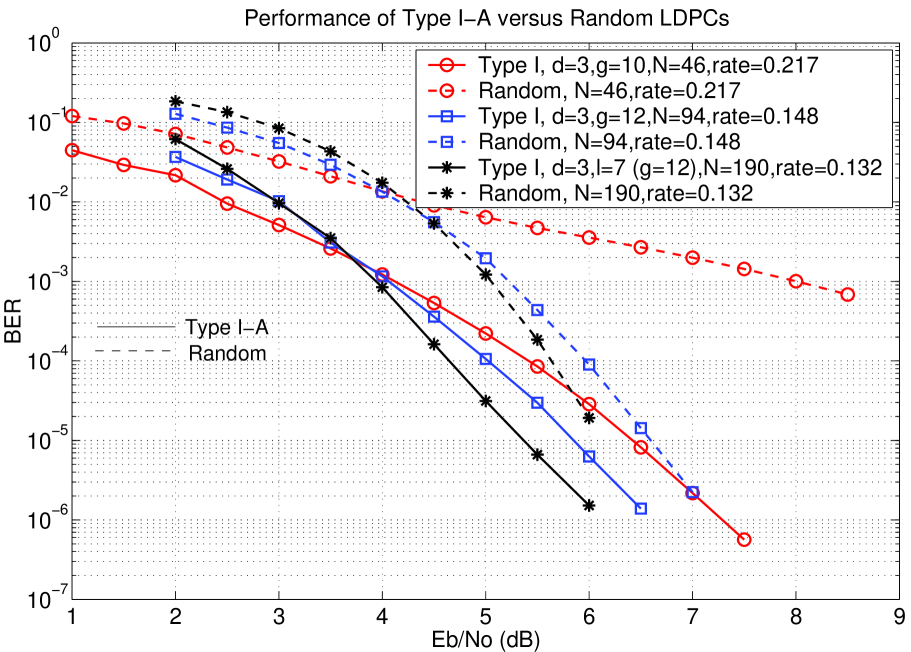
Figure 8: Performance of Type I-A versus Random LDPC codes on the BIAWGNC with min-sum iterative decoding.

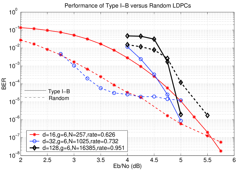
Figure 9: Performance of Type I-B versus Random LDPC codes on the BIAWGNC with min-sum iterative decoding.

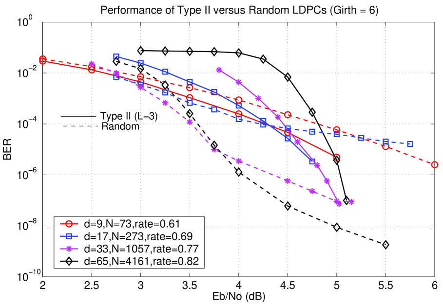
Figure 10: Performance of Type II $\ell=3$ versus Random LDPC codes on the BIAWGNC with min-sum iterative decoding.

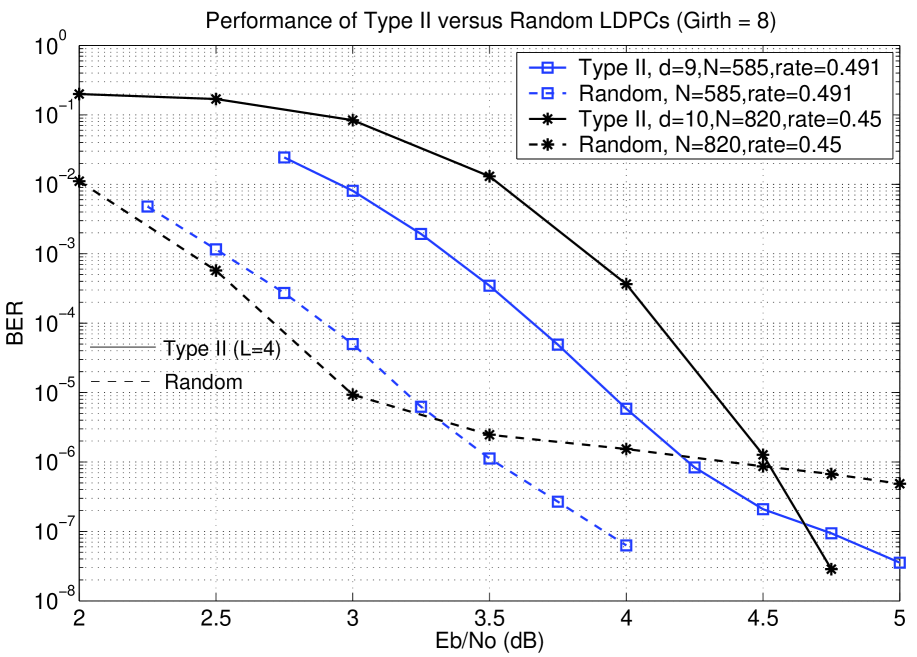
Figure 11: Performance of Type II $\ell=4$ versus Random LDPC codes on the BIAWGNC with min-sum iterative decoding.

Figures 8, 9, 10, 11 show the bit-error-rate performance of Type I-A, Type I-B, Type II $\ell=3$ (girth six), and Type II $\ell=4$ (girth eight) LDPC codes, respectively, over the binary input additive white Gaussian noise channel (BIAWGNC) with min-sum (not, sum-product!) iterative decoding, as a function of the channel signal to noise ratio (SNR) $E_{b}/N_{o}$. The performance of regular or semi-regular randomly constructed LDPC codes of comparable rates and block lengths are also shown. (All of the random LDPC codes compared in this paper have a variable node degree of three and are constructed from the online LDPC software available at http://www.cs.toronto.edu/$\tilde{}$ radford/ldpc.software.html.)

Figure 8 shows that the Type I-A LDPC codes perform substantially better than their random counterparts for all the codes shown. In these simulations, a maximum of 10000 iterations of min-sum decoding were allowed.

Figure 9 reveals that the Type I-B LDPC codes perform better than comparable random LDPC codes at short block lengths; but as the block lengths increase, the random LDPC codes tend to perform better in the waterfall region. Eventually however, as the SNR increases, the Type I-B LDPC codes outperform the random ones and, unlike the random codes, they do not have a prominent error floor. For short block lengths (below 4000), a maximum of 200 decoding iterations were allowed whereas for the longer block lengths, only up to 20 decoding iterations were allowed. The block length 16385, rate 0.951, Type I-B LDPC code performs significantly better than the corresponding random LDPC code of the same block length and rate.

Figure 10 reveals that the performance of Type II $\ell=3$ (girth-six) LDPC codes is also significantly better than comparable random codes; these codes correspond to the two dimensional PG-LDPC codes of [19]. The Type II codes significantly outperform the corresponding random LDPC codes of comparable parameters at short block lengths. At longer block lengths, the random codes tend to perform better in the waterfall region due to their superior minimum distances. A maximum of 200 iterations were allowed for short block length codes (block lengths below 4000) whereas only 20 iterations were allowed for the block length 4161 code. Here again, the Type II codes do not reveal a prominent error as the corresponding random LDPC codes do, and at longer block lengths, they outperform the corresponding random LDPC codes in the high SNR regime.

Figure 11 indicates the performance of Type II $\ell=4$ (girth-eight) LDPC codes; these codes perform comparably to random codes at short block lengths, but at large block lengths, the random codes perform better as they have larger relative minimum distances compared to the Type II $\ell=4$ (girth-eight) LDPC codes. In these simulations, a maximum of 200 decoding iterations were allowed for all the codes shown. The performance of the Type II $\ell=4$ LDPC codes reveal a similar trend as that of the Type II $\ell=3$ LDPC codes in Figure 10.

As a general observation, min-sum iterative decoding of most of the tree-based LDPC codes (particularly, Type I-A, Type II, and some Type I-B) presented here did not typically reveal detected errors, i.e., errors caused due to the decoder failing to converge to any valid codeword within the maximum specified number of iterations, which was set to 200 for short block length codes (and 20 for longer blocklength codes) in these simulations. Detected errors are caused primarily due to the presence of pseudocodewords, especially those of minimum weight. We think that the relatively low occurrences of detected errors with iterative decoding of these LDPC codes is primarily due to their good minimum pseudocodeword weight $w_{\min}$.

V-B Performance of Type I-B and Type II LDPC codes with sum-product iterative decoding

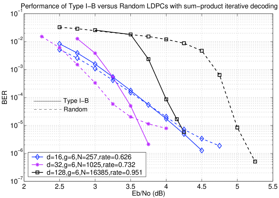
Figure 12: Performance of Type I-B versus Random LDPC codes on the BIAWGNC with sum-product iterative decoding.

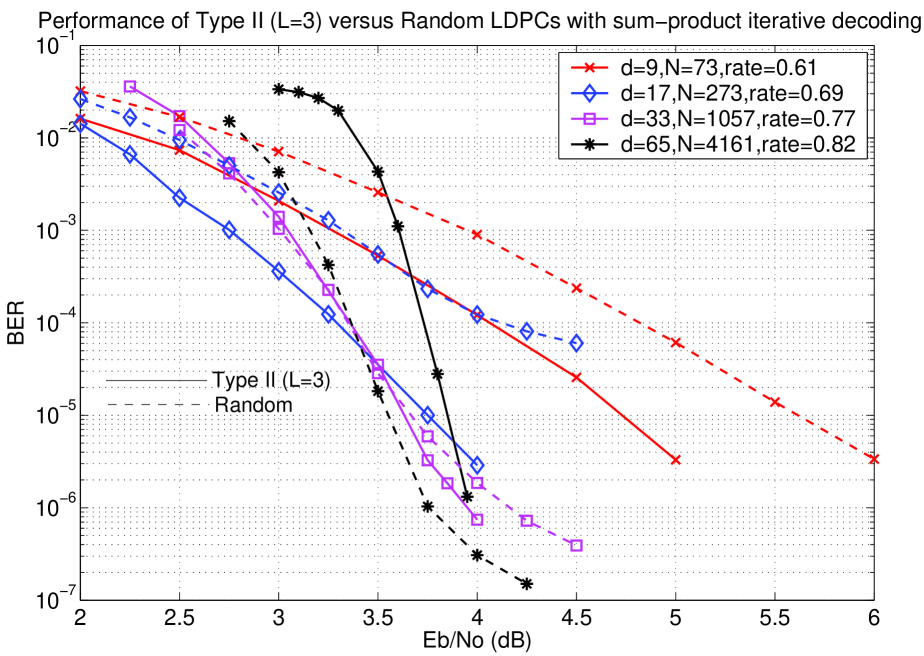
Figure 13: Performance of Type II $\ell=3$ versus Random LDPC codes on the BIAWGNC with sum-product iterative decoding.

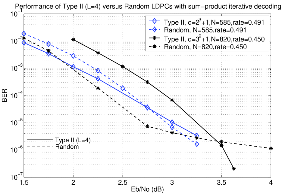
Figure 14: Performance of Type II $\ell=4$ versus Random LDPC codes on the BIAWGNC with sum-product iterative decoding.

Figures  12, 13, and 14 show the performance of the Type I-B, Type II $\ell=3$ and Type II $\ell=4$, respectively, LDPC codes with sum-product iterative decoding for the BIAWGNC. The performance is shown only for a few codes from each construction. The main observation from these performance curves is that the the tree-based LDPC codes perform relatively much better than random LDPC codes of comparable parameters when the decoding is sum-product instead of the min-sum algorithm. Although the Type I-B LDPC codes perform a little inferior to their random counterparts in the waterfall region when the block length is large, the gap between the performances of the random and the Type I-B LDPC codes is much smaller with sum-product decoding than with min-sum decoding. (Compare Figures 9 and 12.) Once again, a maximum of 200 decoding iterations were performed for block lengths below 4000 and 20 decoding iterations were performed for the block length 4097 LDPC code.

Similarly, comparing Figures  13 and 10, we see that the Type II $\ell=3$ LDPC codes perform relatively much better than their random counterparts with sum-product decoding than with min-sum decoding. They outperform the corresponding random LDPC codes at block lengths below 1000, whereas at the longer block lengths, the random codes perform better than the Type II codes in the waterfall region. Figure 14, in comparison with Figure 11, shows a similar trend in performance of Type II $\ell=4$ (girth 8) LDPC codes with sum-product iterative decoding.

Note that the simulation results for the min-sum and sum-product decoding correspond to the case when the LDPC codes resulting from constructions Type I and Type II were treated as binary LDPC codes for all choices of degree $d=p^{s}$ or $d=p^{s}+1$. We will now examine the performance when the codes are treated as $p$-ary codes if the corresponding degree in the LDPC constraint graph is $d=p^{s}$ (for Type I-B) or $d=p^{s}+1$ (for Type II). (Note that this will affect only the performances of those codes for which $p$ is not equal to two.)

V-C Performance of $p$-ary Type I-B and Type II LDPC codes over the $p$-ary symmetric channel

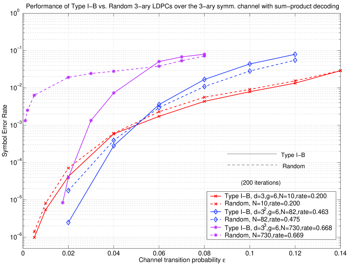
Figure 15: Performance of Type I-B versus Random 3-ary LDPC codes on the 3-ary symmetric channel with sum-product iterative decoding.

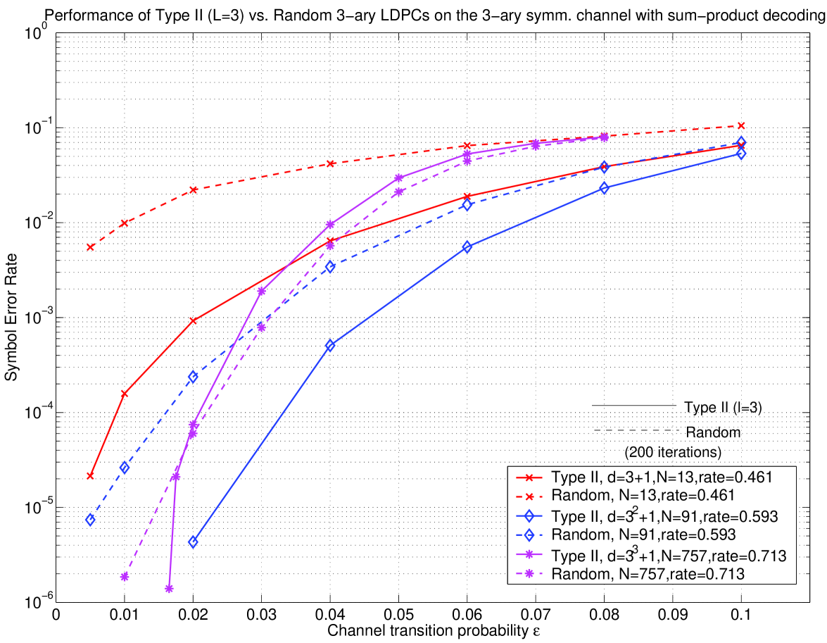
Figure 16: Performance of Type II $\ell=3$ versus Random 3-ary LDPC codes on the 3-ary symmetric channel with sum-product iterative decoding.

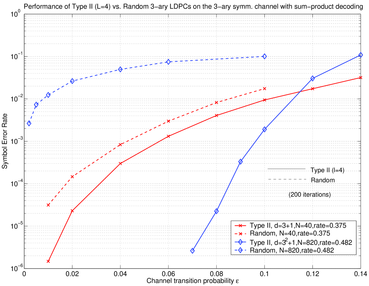
Figure 17: Performance of Type II $\ell=4$ versus Random 3-ary LDPC codes on the 3-ary symmetric channel with sum-product iterative decoding.

We examine the performance of the $p$-ary LDPC codes obtained from the Type I-B and Type II constructions on the $p$-ary symmetric channel instead of the AWGN channel. The $p$-ary symmetric channel is shown in Figure 7. An error occurs with probability $\epsilon$, the channel transition probability. Figures 15, 16, and 17 show the performance of Type I-B, Type II $\ell=3$ and Type II $\ell=4$, $3$-ary LDPC codes, respectively, on the $3$-ary symmetric channel with sum-product iterative decoding. A maximum of 200 sum-product decoding iterations were performed. The parity check matrices resulting from the the Type I-B and Type II constructions are considered to be matrices over the field $GF(3)$ and sum-product iterative decoding is implemented as outlined in [3]. The corresponding plots show the information symbol error rate as a function of the channel transition probability $\epsilon$. In Figure 15, the performance of $3$-ary Type I-B LDPC codes obtained for degrees $d=3$, $d=3^{2}$, and $d=3^{3}$, is shown and compared with the performance of random $3$-ary LDPC codes of comparable rates and block lengths. (To make a fair comparison, the random LDPC codes also have only zeros and ones as entries in their parity check matrices. It has been observed in [3] that choosing the non-zero entries in the parity check matrices of non-binary codes cleverly can yield some performance gain, but this avenue was not explored in these simulations.) In Figure 16, the performance of $3$-ary Type II $\ell=3$ (girth six) LDPC codes obtained for degrees $d=3+1$, $d=3^{2}+1$, and $d=3^{3}+1$, is shown and compared with random $3$-ary LDPC codes. Figure 17 shows the analogous performance of $3$-ary Type II $\ell=4$ (girth eight) LDPC codes obtained for degrees $d=3+1$ and $d=3^{2}+1$. In all these plots, it is seen that the tree-based constructions perform comparably or better than random LDPC codes of similar rates and block lengths. (In some cases, the performance of the tree-based constructions is significantly better than that of random LDPC codes (example, Figure 17).)

The simulation results show that the tree-based constructions yield LDPC codes with a wide range of rates and block lengths that perform very well with iterative decoding.

VI Conclusions

The Type I construction yields a family of LDPC codes that, to the best of our knowledge, do not correspond to any of the LDPC codes obtained from finite geometries or other geometrical objects. It would be interesting to extend the Type II construction to more layers as described at the end of Section 5, and to extend the Type IA construction by relaxing the girth condition. In addition, these codes may be amenable to efficient tree-based encoding procedures. A definition for the pseudocodeword weight of $p$-ary LDPC codes on the $p$-ary symmetric channel was also derived, and an extension of the tree bound in [9] was obtained. This led to a useful interpretation of the tree-based codes, including the projective geometry LDPC codes, for $p>2$. The tree-based constructions presented in this paper yield a wide range of codes that perform well when decoded iteratively, largely due to the maximized minimum pseudocodeword weight. While the tree-based constructions are based on pseudocodewords that arise from the graph-cover’s polytope of [11] and aim to maximize the minimum pseudocodeword weight of pseudocodewords in this set, they do not consider all pseudocodewords arising on the min-sum iterative decoder’s computation tree [26]. Nonetheless, having a large minimal pseudocodeword weight in this set necessarily brings the performance of min-sum iterative decoding of the tree-based codes closer to the maximum-likelihood performance. However, it would be interesting to find other design criteria that account for pseudocodewords arising on the decoder’s computation tree.

Furthermore, since the tree-based constructions have the minimum pseudocodeword weight and the minimum distance close to the tree bound, the overall minimum distance of these codes is relatively small. While this is a first step in constructing LDPC codes having the minimum pseudocodeword weight $w_{\min}$ equal/almost equal to the minimum distance $d_{\min}$, constructing codes with larger minimum distance, while still maintaining $d_{\min}=w_{\min}$, remains a challenging problem.

-A Pseudocodeword weight for $p$-ary LDPC codes on the $p$-ary symmetric channel

Suppose the all-zero codeword is sent across a $p$-ary symmetric channel and the vector ${\bf r}=(r_{0},r_{1},\dots,r_{n-1})$ is received. Then errors occur in positions where $r_{i}\neq 0$. Let $S=\{i|\ r_{i}\neq 0\}$ and let $S^{c}=\{i|\ r_{i}=0\}$. The distance between ${\bf r}$ and a pseudocodeword $F$ is defined as

$$d({\bf r},F)=\sum_{i=0}^{n-1}\sum_{k=0}^{p-1}\chi(r_{i}\neq k)f_{i,k},$$ (2)

where $\chi(P)$ is an indicator function that is equal to $1$ if the proposition $P$ is true and is equal to $0$ otherwise.

The distance between ${\bf r}$ and the all-zero codeword ${\bf 0}$ is

$$d({\bf r},{\bf 0})=\sum_{i=0}^{n-1}\chi(r_{i}\neq 0)$$

which is the Hamming weight of ${\bf r}$ and can be obtained from equation (2).

The iterative decoder chooses in favor of $F$ instead of the all-zero codeword ${\bf 0}$ when $d({\bf r},F)\leq d({\bf r},{\bf 0})$. That is, if

$$\sum_{i\in S^{c}}(1-f_{i,0})+\sum_{i\in S}(1-f_{i,r_{i}})\leq\sum_{i\in S}1$$

The condition for choosing $F$ over the all-zero codeword reduces to

$$\Big{\{}\sum_{i\in S^{c}}(1-f_{i,0})\leq\sum_{i\in S}f_{i,r_{i}}\Big{\}}$$

Hence, we define the weight of a pseudocodeword $F$ in the following manner.

Let $e$ be a number such that the sum of the $e$ largest components in the matrix $F^{\prime}$, say, $f_{i_{1},j_{1}},f_{i_{2},j_{2}},\dots,f_{i_{e},j_{e}}$, exceeds $\sum_{i\neq i_{1},i_{2},\dots,i_{e}}(1-f_{i,0})$. Then the weight of $F$ on the $p$-ary symmetric channel is defined as

$$w_{PSC}(F)=\left\{\begin{array}[]{cc}2e,&\mbox{if }f_{i_{1},j_{1}}+\dots+f_{i_{e},j_{e}}=\sum_{i\neq i_{1},i_{2},\dots,i_{e}}(1-f_{i,0})\\ 2e-1,&\mbox{if }f_{i_{1},j_{1}}+\dots+f_{i_{e},j_{e}}>\sum_{i\neq i_{1},i_{2},\dots,i_{e}}(1-f_{i,0})\end{array}\right.$$

Note that in the above definition, none of the $j_{k}$’s, for $k=1,2,\dots,e$, are equal to zero, and all the $i_{k}$’s, for $k=1,2,\dots,e$, are distinct. That is, we choose at most one component in every row of $F^{\prime}$ when picking the $e$ largest components. The received vector ${\bf r}=(r_{0},r_{1},\dots,r_{n-1})$ that has the following components: $r_{i_{1}}=j_{1},r_{i_{2}}=j_{2},\dots,r_{i_{e}}=j_{e}$, $r_{i}=0$, for $i\notin\{i_{1},i_{2},\dots,i_{e}\}$, will cause the decoder to make an error and choose $F$ over the all-zero codeword.

-B Proof of Lemma III.6

Proof:

Figure 1: Single constraint code.

$({1-f_{i,0}})\leq\sum_{j\neq i}(1-f_{j,0})$

Figure 2: Local tree structure for a $d$-left regular graph.

$d(1-f_{0,0})\leq\sum_{j\in L_{0}}(1-f_{j,0})$,

$d(d-1)(1-f_{0,0})\leq\sum_{j\in L_{1}}(1-f_{j,0})$

$:$

Case: $\frac{g}{2}$ odd. Consider a single constraint node with $r$ variable node neighbors as shown in Figure 2. Then, for $i=0,1,\dots,r-1$ and $k=0,1,\dots,p-1$, the following inequality holds:

$$f_{i,k}\leq\sum_{j\neq i}\sum_{\sigma_{j}:\sum\sigma_{j}+k=0\mbox{ mod }p}\frac{f_{j,\sigma_{j}}\sigma_{j}}{\sum\sigma_{j}}$$

where the middle summation is over all possible assignments $\sigma_{j}\in\{0,1,\dots,p-1\}$ to the variable nodes $j\neq i$ such that $k+\sum_{j\neq i}\sigma_{j}=0\mbox{ mod }p$, i.e., this is a valid assignment for the constraint node. The innermost summation in the denominator is over all $j\neq i$.

However, for $i=0,1,\dots,r-1$, the following (weaker) inequality also holds:

$$(1-f_{i,0})\leq\sum_{j\neq i}(1-f_{j,0})$$ (3)

Now let us consider a $d$-left regular LDPC constraint graph representing a $p$-ary LDPC code. We will enumerate the LDPC constraint graph as a tree from an arbitrary root variable node, as shown in Figure 2. Let $F$ be a pseudocodeword matrix for this graph. Without loss of generality, let us assume that the component $(1-f_{0,0})$ corresponding to the root node is the maximum among all $(1-f_{i,0})$ over all $i$.

Applying the inequality in (3) at every constraint node in first constraint node layer of the tree, we obtain

$$d(1-f_{0,0})\leq\sum_{j\in L_{0}}(1-f_{j,0}),$$

where $L_{0}$ corresponds to variable nodes in first level of the tree. Subsequent application of the inequality in (3) to the second layer of constraint nodes in the tree yields

$$d(d-1)(1-f_{0,0})\leq\sum_{j\in L_{1}}(1-f_{j,0}),$$

Continuing this process until layer $L_{\frac{g-6}{4}}$, we obtain

$$d(d-1)^{\frac{g-6}{4}}(1-f_{0,0})\leq\sum_{j\in L_{\frac{g-6}{4}}}(1-f_{j,0})$$

Since the LDPC graph has girth $g$, the variable nodes up to level $L_{\frac{g-6}{4}}$ are all distinct. The above inequalities yield:

$$[1+d+d(d-1)+\dots+d(d-1)^{\frac{g-6}{4}}](1-f_{0,0})\leq\sum_{i\in\{0\}\cup L_{0}\cup\dots L_{\frac{g-6}{4}}}(1-f_{i,0})\leq\sum_{\mbox{ all }i}(1-f_{i,0})$$ (4)

Let $e$ the smallest number such that there are $e$ maximal components $f_{i_{1},j_{1}}$, $f_{i_{2},j_{2}},f_{i_{3},j_{3}},\dots,f_{i_{e},j_{e}}$, for $i_{1},i_{2},\dots,i_{e}$ all distinct and $j_{1},j_{2},\dots,j_{e}\in\{1,2,\dots,p-1\}$, in $F^{\prime}$ (the sub-matrix of $F$ excluding the first column in $F$) such that

$$f_{i_{1},j_{1}}+f_{i_{2},j_{2}}+\dots+f_{i_{e},j_{e}}\geq\sum_{i\notin\{i_{1},i_{2},i_{3},\dots,i_{e}\}}(1-f_{i,0})$$

Then, since none of the $j_{k}$’s, $k=1,2,\dots,e$, are zero, we clearly have

$$(1-f_{i_{1},0})+(1-f_{i_{2},0})+\dots+(1-f_{i_{e},0})\geq f_{i_{1},j_{1}}+f_{i_{2},j_{2}}+\dots+f_{i_{e},j_{e}}\geq\sum_{i\notin\{i_{1},i_{2},i_{3},\dots,i_{e}\}}(1-f_{i,0})$$

Hence we have that

$$2((1-f_{i_{1},0})+(1-f_{i_{2},0})+\dots+(1-f_{i_{e},0}))\geq\sum_{\mbox{all }i}(1-f_{i,0})$$

We can then lower bound this further using the inequality in (4) as

$$2((1-f_{i_{1},0})+(1-f_{i_{2},0})+\dots+(1-f_{i_{e},0}))\geq[1+d+d(d-1)+\dots+d(d-1)^{\frac{g-6}{4}}](1-f_{0,0})$$

Since we assumed that $(1-f_{0,0})$ is the maximum among $(1-f_{i,0})$ over all $i$, we have

$$2e(1-f_{0,0})\geq 2((1-f_{i_{1},0})+(1-f_{i_{2},0})+\dots+(1-f_{i_{e},0}))\geq[1+d+d(d-1)+\dots+d(d-1)^{\frac{g-6}{4}}](1-f_{0,0})$$

This yields the desired bound

$$w_{PSC}(F)=2e\geq 1+d+d(d-1)+\dots+d(d-1)^{\frac{g-6}{4}}$$

Since the pseudocodeword $F$ was arbitrary, we also have $w_{min}\geq 1+d+d(d-1)+\dots+d(d-1)^{\frac{g-6}{4}}$. The case $\frac{g}{2}$ even is treated similarly.
∎

-C Table of code parameters

The code parameters resulting from the tree-based constructions are summarized in Tables IV, IV, VI, and  VI. Note that ^∗ indicates an upper bound instead of the exact minimum distance (or minimum pseudocodeword weight) since it was computationally hard to find the distance (or pseudoweight) for those cases. Similarly, for cases where it was computationally hard to get any reasonable bound the minimum pseudocodeword weight, the corresponding entry in the table is left empty. The lower bound on $w_{\min}$ seen in the tables corresponds to the tree bound (Theorem I.2). It is observed that when the codes resulting from the construction are treated as $p$-ary codes rather than binary codes when the corresponding degree in the LDPC graph is $d=p^{s}$ (for Type I-B) or $d=p^{s}+1$ (for Type II), the resulting rates obtained are much superior; we also believe that the minimum pseudocodeword weights (on the $p$-ary symmetric channel) are much closer to the minimum distances for these $p$-ary LDPC codes.

No. of layers in $T$	block length	degree	dimension	rate	$d_{\min}$	$w_{\min}$	tree	girth	diameter
$\ell$	$n$	$d=3$					lower-bound	$g$	$\delta$
3	10	3	4	0.4000	4	4	4	6	5
4	22	3	4	0.1818	8	$8^{*}$	6	8	7
5	46	3	10	0.2173	10	10	10	10	9
6	94	3	14	0.1489	20	$20^{*}$	18	12	11
7	190	3	25	0.1315	24	$\geq 18$	18	12	13

TABLE III: Summary of Type I-A code parameters.

$p$	$s$	block length	degree	dimension	rate	$d_{\min}$	$w_{\min}$	tree	girth	diameter	code
		$n=p^{2s}+1$	$d=p^{s}$					lower-bound	$g$	$\delta$	alphabet
2	1	5	2	1	0.2000	5	5	4	8	4	binary
3	1	10	3	3	.3000	4	4	4	6	5	binary
				(2)	(0.2000)	(6)	( )				3-ary
2	2	17	4	5	0.2941	6	$6^{*}$	5	6	5	binary
5	1	26	5	7	0.2692	8	$8^{*}$	6	6	5	binary
				(7)	(0.2692)	(10)	( )				5-ary
7	1	50	7	11	0.2200	12	$12^{*}$	8	6	5	binary
				(16)	(0.3200)	($15$)	( )				7-ary
2	3	65	8	31	0.4769	$10$	$10^{*}$	9	6	5	binary
3	2	82	9	15	0.1829	16	$\geq 10$	10	6	5	binary
				(38)	(0.4634)	$(15)$	( )				3-ary
11	1	122	11	19	0.1557	$20^{*}$	$\geq 12$	12	6	5	binary
				(46)	(0.3770)	($30^{*}$)	( )				11-ary
2	4	257	16	161	0.6264	$20^{*}$	$\geq 17$	17	6	5	binary
5	2	626	25	47	0.075	$48^{*}$	$\geq 26$	26	6	5	binary
				(377)	(0.6022)	($90^{*}$)	( )				5-ary
3	3	730	27	51	0.0698	$52^{*}$	$\geq 28$	28	6	5	binary
				(488)	(0.6684)	($60^{*}$)	( )				3-ary
2	5	1025	32	751	0.7326	$40^{*}$	$\geq 33$	33	6	5	binary
7	2	2404	49	95	0.0395	$96^{*}$	$\geq 50$	50	6	5	binary
				(1572)	(0.6536)	($216^{*}$)	( )				7-ary

TABLE IV: Summary of Type I-B code parameters.

$p$	$s$	block length	degree	dimension	rate	$d_{\min}$	$w_{\min}$	tree	girth	diameter	code
		$n=1+p^{s}+p^{2s}$	$d=p^{s}+1$					lower-bound	$g$	$\delta$	alphabet
2	1	7	3	3	0.4285	4	4	4	6	3	binary
3	1	13	4	1	0.0769	13	$6^{*}$	5	6	3	binary
				(6)	(0.4615)	(6)	( )				3-ary
2	2	21	5	11	0.5238	6	6	6	6	3	binary
5	1	31	6	1	0.0322	31	$10^{*}$	7	6	3	binary
				(15)	(0.4838)	($10^{*}$)	( )				5-ary
7	1	57	8	1	0.017	57	$16^{*}$	9	6	3	binary
				(28)	(0.4912)	($14^{*}$)	( )				7-ary
2	3	73	9	45	0.6164	10	10	10	6	3	binary
3	2	91	10	1	0.0109	91	$\geq 11$	11	6	3	binary
				(54)	(0.5934)	($15^{*}$)	( )				3-ary
2	4	273	17	191	0.6996	18	18	18	6	3	binary
5	2	651	26	1	0.0015	651	$\geq 27$	27	6	3	binary
				(425)	(0.6528)	($56^{*}$)	( )				5-ary

TABLE V: Summary of Type II, $\ell=3$ code parameters.

$p$	$s$	block length	degree	dimension	rate	$d_{\min}$	$w_{\min}$	tree	girth	diameter	code
		$n$=$1$+$p^{s}$+$p^{2s}$+$p^{3s}$	$d$=$p^{s}$+$1$					lower-bound	$g$	$\delta$	alphabet
2	1	15	3	5	0.3333	6	6	6	8	4	binary
3	1	40	4	15	0.3750	10	$\geq 8$	8	$8$	4	binary
				(15)	(0.3750)	($10^{*}$)	( )				3-ary
2	2	85	5	35	0.4117	10	10	10	8	4	binary
5	1	156	6	65	0.4167	$20^{*}$	$\geq 12$	12	8	4	binary
				(65)	(0.4167)	($26^{*}$)	( )				5-ary
7	1	400	8	175	0.4375	$66^{*}$	$\geq 16$	16	8	4	binary
				(175)	(0.4375)	($119^{*}$)	( )				7-ary
2	3	585	9	287	0.4905	18	18	18	8	4	binary
3	2	820	10	369	0.4500	$112^{*}$	$\geq 20$	20	8	4	binary
				(395)	(0.4817)	($96^{*}$)	( )				3-ary

TABLE VI: Summary of Type II, $\ell=4$ code parameters.

Figure 3: Type I-A LDPC constraint graph having degree $d=3$ and girth $g=10$.

Figure 4: Type I-B LDPC constraint graph having degree $d=4$ and girth $g=6$.

Figure 5: Type II LDPC constraint graph having degree $d=4$ and girth $g=6$.

Figure 6: Type II LDPC constraint graph having degree $d=3$ and girth $g=8$. (Shaded nodes highlight a minimum weight codeword.)

Figure 7: A $p$-ary symmetric channel.

References

- [1] N. L. Biggs. Construction for cubic graphs of large girths. Electronic Journal of Combinatorics, 5, 1998.
- [2] R. C. Bose. On the application of the properties of Galois fields to the problem of construction of Hyper-Graceo-Latin squares. Sankhy, pages 323–338, 1938.
- [3] M. C. Davey. Error-correction using Low-Density Parity-Check Codes. PhD thesis, University of Cambridge, 1999.
- [4] M. C. Davey and D. J. C. MacKay. Low density parity check codes over GF(q). IEEE Communications Letters, 2(6):159–166, June 1998.
- [5] C. Di, D. Proietti, I. E. Teletar, T. Richardson, and R. Urbanke. Finite-length analysis of low-density parity-check codes on the binary erasure channel. IEEE Trans. Inform. Theory, 48(2):1570–1579, 2002.
- [6] G. D. Forney, Jr., R. Koetter, F. Kschischang, and A. Reznik. On the effective weights of pseudocodewords for codes defined on graphs with cycles. In B. Marcus and J. Rosenthal, editors, Codes, Systems and Graphical Models, IMA Vol. 123, pages 101–112. Springer-Verlag, 2001.
- [7] J. Han and P. H. Siegel. Improved upper bounds on stopping redundancy. Submitted to the IEEE Transactions on Information Theory, Nov. 2005, http://arxiv.org/abs/cs/0511056.
- [8] N. Kashyap and A. Vardy. Stopping sets in codes from designs. In Proceedings of the 2003 IEEE International Symposium on Information Theory, Yokohama, Japan, p. 122, July 2003.
- [9] C. A. Kelley and D. Sridhara. Pseudocodewords of Tanner graphs. Submitted to IEEE Trans. on Information Theory, June 2005.
- [10] C. A. Kelley, D. Sridhara, J. Xu, and J. Rosenthal. Pseudocodeword Weights and Stopping Sets. In Proc. of the IEEE International Symposium on Information Theory, (Chicago, USA), page 150, 2004.
- [11] R. Koetter and P. O. Vontobel. Graph-covers and iterative decoding of finite length codes. In Proceedings of the IEEE International Symposium on Turbo Codes and Applications, Brest, France, September 2003.
- [12] Y. Kou, S. Lin, and M. P. C. Fossorier. Low-density parity-check codes based on finite geometries: a rediscovery and new results. IEEE Trans. Inform. Theory, 47(7):2711–2736, 2001.
- [13] MAGMA Software. Documentation available at http://magma.maths.usyd.edu.
- [14] R. L. Graham and F. J. MacWilliams. On the number of information symbols in difference-set cyclic codes. Bell Labs Technical Journal, 45:10571070, 1966.
- [15] H. van Maldeghem. Generalized Polygons. Birkhäuser Verlag, Basel, Boston, Berlin, 1998.
- [16] F. S. Roberts. Applied Combinatorics. Prentice Hall Inc., Englewood Cliffs, NJ, 1984.
- [17] L. Rudolph. A class of majority logic decodable codes. IEEE Trans. Inform. Theory, IT-13(2):305–307, April 1967.
- [18] D. Sridhara and T. E. Fuja. LDPC codes over rings for PSK-modulation. IEEE Trans. Inform. Theory, IT-51(9):3209–3220, 2005.
- [19] H. Tang, J. Xu, S. Lin, and K. A. S. Abdel-Ghaffar. Codes on finite geometries. IEEE Trans. Inform. Theory, IT-51(2):572–596, 2005.
- [20] R. M. Tanner. A recursive approach to low complexity codes. IEEE Trans. Inform. Theory, 27(5):533–547, 1981.
- [21] J. H. van Lint and R. M. Wilson. A Course in Combinatorics. Cambridge University Press, second edition, 2001.
- [22] J. Rosenthal and P. O. Vontobel. Constructions of LDPC codes using Ramanujan graphs and ideas from Margulis, In Proc. of the 38-th Allerton Conference on Communication, Control, and Computing, 2000, pp. 248–257.
- [23] M. Schwartz and A. Vardy. On the stopping distance and the stopping redundancy of codes. IEEE Trans. Inform. Theory, IT-52(3):922 - 932, March 2006.
- [24] R. M. Tanner, D. Sridhara, A. Sridharan, D.J. Costello, Jr., and T. E. Fuja. LDPC block and convolutional codes based on circulant matrices. IEEE Trans. Inform. Theory, 50(12):2966–2984, 2004.
- [25] P. O. Vontobel and R. M. Tanner. Construction of codes based on finite generalized quadrangles for iterative decoding. In Proceedings of the 2001 IEEE International Symposium on Information Theory, page 223, Washington, D.C., 2001.
- [26] N. Wiberg. Codes and Decoding on General Graphs. PhD thesis, Linköping University, Sweden, 1996.