Real Hypercomputation and Continuity

Abstract

By the sometimes so-called Main Theorem of Recursive Analysis, every computable real function is necessarily continuous. We wonder whether and which kinds of hypercomputation allow for the effective evaluation of also discontinuous $f:\mathbb{R}\to\mathbb{R}$. More precisely the present work considers the following three super-Turing notions of real function computability:

• relativized computation;  specifically given oracle access to the Halting Problem $\emptyset^{\prime}$ or its jump $\emptyset^{\prime\prime}$;

• encoding input $x\in\mathbb{R}$ and/or output $y=f(x)$ in weaker ways also related to the Arithmetic Hierarchy;

• non-deterministic computation.

It turns out that any $f:\mathbb{R}\to\mathbb{R}$ computable in the first or second sense is still necessarily continuous whereas the third type of hypercomputation does provide the required power to evaluate for instance the discontinuous Heaviside function.

1 Motivation

What does it mean for a Turing Machine, capable of operating only on discrete objects, to compute a real number $x$:

$\boldsymbol{\rho_{\text{b},2}}$:	To determine its binary expansion, i.e., to decide $A\subseteq\mathbb{N}$ with $x=\sum\limits_{n\in A}2^{-n}$ ?
$\boldsymbol{\rho_{\text{Cn}}}$:	To compute a sequence $(q_{n})$ of rational numbers eventually converging to $x$?
$\boldsymbol{\rho}$:	To compute a fast convergent sequence $(q_{n})\subseteq\mathbb{Q}$ for $x$,  i.e. with $|x-q_{n}|$
	$\leq 2^{-n}$   (in other words: to approximate $x$ with effective error bounds)?
$\boldsymbol{\rho_{\raisebox{0.60275pt}{${\scriptscriptstyle<}$}}}$:	To approximate $x$ from below, i.e., to compute $(q_{n})$ such that $x=\sup_{n}q_{n}$ ?

All these notions make sense in being closed under arithmetic operations like addition and multiplication. In fact they are well (known equivalent to variants) studied in literature; e.g. [Tur36], [BH02], [Tur37], [Wei01] in order.

Now what does it mean for a Turing Machine $\mathcal{M}$ to compute a real function $f:\mathbb{R}\to\mathbb{R}$? Most naturally it means that $\mathcal{M}$ realizes effective evaluation $x\mapsto f(x)$ in that, upon input of $x\in\mathbb{R}$ given in one of the above ways, it outputs $y=f(x)$ also in one (not necessarily the same) of the above ways. And, again, many possible combinations have already been investigated. For instance the standard notion of real function computation in Recursive Analysis [Grz57, PER89, Ko91, Wei01] refers (or is equivalent) to input and output given according to $\rho$. Here, the Main Theorem of Computable Analysis implies that any computable $f$ will necessarily be continuous [Wei01, Theorem 4.3.1].

We are interested in ways of lifting this restriction, that is, in the following

Question 1

Does hypercomputation in some sense permit the computational evaluation of (at least certain) discontinuous real functions?

That is related to the Church-Turing Hypothesis: A Turing Machine’s ability to simulate every physical process would imply all such processes to behave continuously—a property G. Leibniz was convinced of (“Natura non facit saltus”) but which we nowadays know to be violated for instance by the Quantum Hall Effect awarded a Nobel Prize in 1985. Since this (nor any other) discontinuous physical process cannot be simulated on a classical Turing Machine, it constitutes a putative candidate for a system capable of realizing hypercomputation.

1.1 Summary

The standard (and indeed the most general) way of turning a Turing Machine into a hypercomputer is to grant it access to an oracle like, say, the Halting Problem $\emptyset^{\prime}$ or its iterated jumps like $\emptyset^{\prime\prime}$ and $\emptyset^{(d)}$ in Kleene’s Arithmetic Hierarchy. However regarding computational evaluation of real functions, closer inspection in Section 3.1 reveals that this Main Theorem relies solely on information rather than recursion theoretic arguments and therefore requires continuity also for oracle-computable real functions with respect to input and output of form $\rho$. (For the special case of an $\emptyset^{\prime}$–oracle, this had been observed in [Ho99, Theorem 16].)

A second idea, applicable to real but not to discrete computability, changes the input and output representation for $x$ and $y=f(x)$ from $\rho$ to a weaker form like, say, $\rho_{\text{Cn}}$. This relates to the Arithmetic Hierarchy, too, however in a different way: Computing $x$ in the sense of $\rho_{\text{Cn}}$ is equivalent to computing $x$ in the sense of $\rho$ [Ho99, Theorem 9] relative (i.e., given access) to the Halting Problem $\emptyset^{\prime}$ and thus suggests to write $\rho^{\prime}:=\rho_{\text{Cn}}$. Most promisingly, the Main Theorem [Wei01, Corollary 3.2.12] which requires continuity of $(\rho\to\rho)$–computable real functions applies to $\rho$ but not to $\rho^{\prime}$ because the latter lacks the technical property of admissibility.

It therefore came to quite a surprise when Brattka and Hertling established that any $(\rho^{\prime}\to\rho^{\prime})$–computable $f$ (that is, with respect to input $x$ and output $f(x)$ encoded according to $\rho_{\text{Cn}}$) still satisfies continuity; see [Wei01, Exercise 4.1.13d] or [BH02, Section 6].

Section 3.2 contains an extension of this and a series of related results. Specifically we manage to prove that continuity is necessary for $(\rho^{\prime\prime}\to\rho^{\prime\prime})$–computability of $f$; here,  $\rho\>\precneq\>\rho^{\prime}\>\precneq\>\rho^{\prime\prime}\>\precneq\ldots$  denote the first levels of an entire hierarchy of real number representations explained in Lemma 1 which emerge naturally from the Real Arithmetic Hierarchy of Weihrauch and Zheng [ZW01].

In Section 4, we closer investigate the two approaches to real function hypercomputation. Specifically it is established (Section 4.1) that the hierarchy of real number representation actually does yield a hierarchy of weakly computable real functions. Furthermore a comparison of both oracle-supported and weakly computable (and each hence necessarily continuous) real functions in Section 4.2 reveals a relativized version of the Effective Weierstraß Theorem to fail.

Our third approach to real hypercomputation (Section 5) finally allows the Turing Machines under consideration to behave nondeterministically. Remarkably and in contrast to the classical (Type-1) theory, this does significantly increase their principal capabilities. For example, all quasi-strongly $\delta$–$\mathbb{Q}$–analytic functions in the sense of Chadzelek and Hotz [CH99]—and in particular many discontinuous real functions—now become computable as well as conversion among the aforementioned representations $\rho_{\text{Cn}}$ and $\rho_{\text{b},2}$.

2 Arithmetic Hierarchy and Reals

In [Ho99], Ho observed an interesting relation between computability of a real number $x$ in the respective senses of $\rho$ and $\rho_{\text{Cn}}$ in terms of oracles: $x=\lim_{n}q_{n}$ for an (eventually convergent) computable rational sequence $(q_{n})$  iff  $x$ admits a fast convergent rational sequence computable with oracle $\emptyset^{\prime}$, that is, a sequence $(p_{m})\subseteq\mathbb{Q}$ recursive in $\emptyset^{\prime}$ with $|x-p_{m}|\leq 2^{-m}$. This suggests to use $\rho^{\prime}$ synonymously for $\rho_{\text{Cn}}$; and denoting by $\Delta_{1}\mathbb{R}=\mathbb{R}_{c}$ the set of reals computable in the sense of Recursive Analysis (that is with respect to $\rho$), it is therefore natural to write, in analogy to Kleene’s classical Arithmetic Hierarchy, $\Delta_{2}\mathbb{R}$ for the set of all $x\in\mathbb{R}$ computable with respect to $\rho^{\prime}$. Weihrauch and Zheng extended these considerations and obtained for instance [ZW01, Corollary 7.3] the following characterization of $\Delta_{3}\mathbb{R}$: A real $x\in\mathbb{R}$ admits a fast convergent rational sequence recursive in $\emptyset^{\prime\prime}$ iff $x$ is computable in the sense of $\rho^{\prime\prime}$ defined as follows:

$\boldsymbol{\rho^{\prime\prime}}$:

$\displaystyle x=\lim\nolimits_{i}\lim\nolimits_{j}q_{\scriptscriptstyle\langle i,j\rangle}$  for some computable rational sequence $(q_{n})$

where $\langle\cdots\rangle:\mathbb{N}^{*}\to\mathbb{N}$ denotes some fixed computable pairing or, more generally, tupling function. Similarly, $\Sigma_{1}\mathbb{R}$ contains of all $x\in\mathbb{R}$ computable with respect to $\rho_{\raisebox{0.60275pt}{${\scriptscriptstyle<}$}}$ whereas $\Sigma_{2}\mathbb{R}$ includes all $x$ computable in the sense of $\rho_{\raisebox{0.60275pt}{${\scriptscriptstyle<}$}}^{\prime}$ defined as follows:

$\boldsymbol{\rho_{\raisebox{0.60275pt}{${\scriptscriptstyle<}$}}^{\prime}}$:

$\displaystyle x=\operatorname*{\smash{\sup}}\nolimits_{i}\operatorname*{\smash{\inf}}\nolimits_{j}q_{\scriptscriptstyle\langle i,j\rangle}$  for some computable rational sequence $(q_{n})$.

To $\Sigma_{2}\mathbb{R}$ belongs for instance the radius of convergence $r=1/\limsup_{n\to\infty}\sqrt[n]{a_{n}}$ of a computable power series $\sum_{n=0}^{\infty}a_{n}x^{n}$ [ZW01, Theorem 6.2]. More generally we take from [ZW01, Definition 7.1 and Corollary 7.3] the following

Definition 1 (Real Arithmetic Hierarchy)

Let $d=0,1,2,\ldots$
$\boldsymbol{\rho_{\raisebox{0.60275pt}{${\scriptscriptstyle<}$}}^{(d)}}$: $\Sigma_{d+1}\mathbb{R}$ consists of all $x\in\mathbb{R}$ of the form   $\displaystyle x\;=\;\operatorname*{\smash{\sup}}_{n_{1}}\;\operatorname*{\smash{\inf}}_{n_{2}}\;\ldots\;\operatorname*{\Theta}_{n_{d+1}}\;q_{\scriptscriptstyle\langle n_{1},\ldots,n_{d+1}\rangle}$ for a computable rational sequence $(q_{n})$, where $\operatorname*{\Theta}\!\!=\!\operatorname*{\smash{\sup}}$ or $\operatorname*{\Theta}\!\!=\!\operatorname*{\smash{\inf}}$ depending on $d$’s parity; $\boldsymbol{\rho_{\raisebox{0.60275pt}{${\scriptscriptstyle>}$}}^{(d)}}$: $\Pi_{d+1}\mathbb{R}$ similarly for  $\displaystyle x=\operatorname*{\smash{\inf}}_{n_{1}}\operatorname*{\smash{\sup}}_{n_{2}}\;\ldots$ $\boldsymbol{\rho^{(d)}}$: $\Delta_{d+1}\mathbb{R}$ contains all $x\in\mathbb{R}$ of the form  $\displaystyle x\;=\;\lim_{n_{1}}\;\lim_{n_{2}}\;\ldots\;\lim_{n_{d}}\;q_{\scriptscriptstyle\langle n_{1},\ldots,n_{d}\rangle}$ for a computable rational sequence $(q_{n})$.

(For an extension to levels beyond $\omega$ see [Bar03]…)

The close analogy between the discrete and this real variant of the Arithmetic Hierarchy is expressed in [ZW01] by a variety of elegant results like, e.g.,

Fact 2.1

1. $x\in\Delta_{d}\mathbb{R}$  iff  deciding its binary expansion is in $\Delta_{d}$.

2. $x$ is computable with respect to $\rho^{(d)}$
    iff  there is a $\emptyset^{(d)}$–computable fast convergent rational sequence for $x$.

3. $x$ is computable with respect to $\rho_{\raisebox{0.60275pt}{${\scriptscriptstyle<}$}}^{(d)}$
    iff  $x$ is the supremum of a $\emptyset^{(d)}$–computable rational sequence.

4. $\Delta_{d}\mathbb{R}\;=\;\Sigma_{d}\mathbb{R}\,\cap\,\Pi_{d}\mathbb{R}$.

5. $\Sigma_{d}\mathbb{R}\,\cup\,\Pi_{d}\mathbb{R}\;\subsetneq\;\Delta_{d+1}\mathbb{R}$.

Proof

a) Theorem 7.8, b+c) Lemma 7.2, d) Definition 7.1, and e) Theorem 7.8 in [ZW01], respectively. ∎

2.1 Type-2 Theory of Effectivity

Specifying an encoding formalizes how to feed some general form of input like graphs or integers into a Turing Machine with fixed alphabet $\Sigma$. Already in the discrete case, the complexity of a problem usually depends heavily on the chosen encoding; e.g., numbers in unary versus binary. This dependence becomes even more important when dealing with objects from a continuum like the set of reals and their computability. While Recursive Analysis usually considers one particular encoding for $\mathbb{R}$, the Type-2 Theory of Effectivity (TTE) due to Weihrauch provides (a convenient formal framework for studying and comparing) a variety of encodings for different universes. Formally speaking, a representation $\alpha$ for $\mathbb{R}$ is a partial surjective mapping $\alpha:\subseteq\Sigma^{\omega}\to\mathbb{R}$; and an infinite string $\bar{\sigma}\in\operatorname{dom}(\alpha)$ is regarded as an $\alpha$–name for the real number $x=\alpha(\bar{\sigma})$.

In this way, $(\alpha\to\beta)$–computing a real function $f:\mathbb{R}\to\mathbb{R}$ means to compute a transformation on infinite strings $F:\subseteq\Sigma^{\omega}\to\Sigma^{\omega}$ such that any $\alpha$–name $\bar{\sigma}$ for $x=\alpha(\bar{\sigma})$ gets transformed to a $\beta$–name $\bar{\tau}=F(\bar{\sigma})$ for $f(x)=y$, that is, satisfying $\beta(\bar{\tau})=y$; cf. [Wei01, Section 3]. Converting $\alpha$–names to $\beta$–names thus amounts to $(\alpha\to\beta)$–computability of $\operatorname{id}:\mathbb{R}\to\mathbb{R}$, $x\mapsto x$, and is called reducibility “$\alpha\preceq\beta$” [Wei01, Definition 2.3.2]. Computational equivalence, that is mutual reducibility  $\alpha\preceq\beta$ and $\beta\preceq\alpha$, is denoted by “$\alpha\equiv\beta$” whereas “$\alpha\precneq\beta$” means $\alpha\preceq\beta$ but $\beta\not\preceq\alpha$.

We borrow from TTE also two ways of constructing new representations from giving ones: The conjunction $\alpha\wedge\tilde{\alpha}$ of $\alpha$ and $\tilde{\alpha}$ is the least upper bound with respect to “ $\preceq\!$” [Wei01, Lemma 3.3.8]; and for (finitely or countably many) representations $\alpha_{i}:\subseteq\Sigma^{\omega}\to A_{i}$, their product $\prod_{i}\alpha_{i}$ denotes a natural representation for the set $\prod_{i}A_{i}$ [Wei01, Definition 3.3.3.2]. In particular, in order to encode $x\in\mathbb{R}$ as a rational sequence $(q_{n})\in\mathbb{Q}^{\omega}$, we (often implicitly) refer to the representation $[\nu_{\mathbb{Q}}]^{\omega}:\subseteq\Sigma^{\omega}\to\mathbb{Q}^{\omega}$ due to [Wei01, Definition 3.1.2.4 and Lemma 3.3.16].

2.2 Arithmetic Hierarchy of Real Representations

Observe that (the characterizations due to Fact 2.1 of) each level of the Real Arithmetic Hierarchy gives rise not only to a notion of computability for real numbers but also canonically to a representation for $\mathbb{R}$; for instance let

$\boldsymbol{\rho}$  :	encode (arbitrary!) $x\in\mathbb{R}$ as a fast convergent rational sequence $(q_{n})$;
$\boldsymbol{\rho_{\raisebox{0.60275pt}{${\scriptscriptstyle<}$}}}$  :	encode $x\in\mathbb{R}$ as a rational sequence $(q_{n})$ with supremum $x=\sup_{n}q_{n}$;
$\boldsymbol{\rho^{\prime}}$  :	encode $x\in\mathbb{R}$ as a rational sequence $(q_{n})$ with limit $x=\lim_{n}q_{n}$;
$\boldsymbol{\rho_{\raisebox{0.60275pt}{${\scriptscriptstyle<}$}}^{\prime}}$  :	encode $x\in\mathbb{R}$ as $(q_{n})\subseteq\mathbb{Q}$ with $x=\operatorname*{\smash{\sup}}_{i}\operatorname*{\smash{\inf}}_{j}q_{\scriptscriptstyle\langle i,j\rangle}$;
$\boldsymbol{\rho^{\prime\prime}}$  :	encode $x\in\mathbb{R}$ as $(q_{n})\subseteq\mathbb{Q}$ with $x=\lim_{i}\lim_{j}q_{\scriptscriptstyle\langle i,j\rangle}$.

As already pointed out, the first three of them are already known and used in TTE as $\rho$, $\rho_{\raisebox{0.60275pt}{${\scriptscriptstyle<}$}}$, and $\rho_{\text{Cn}}$, respectively [Wei01, Section 4.1]. In general one obtains, similar to Definition 1, a hierarchy of real representations as follows:

Definition 2

Let  $\rho^{(0)}:=\rho$,  $\rho_{\raisebox{0.60275pt}{${\scriptscriptstyle<}$}}^{(0)}:=\rho_{\raisebox{0.60275pt}{${\scriptscriptstyle<}$}}$,  $\rho_{\raisebox{0.60275pt}{${\scriptscriptstyle>}$}}^{(0)}:=\rho_{\raisebox{0.60275pt}{${\scriptscriptstyle>}$}}$.   Now fix $1\leq d\in\mathbb{N}$:
A $\rho^{(d)}$–name for $x\in\mathbb{R}$ is (a $[\nu_{\mathbb{Q}}]^{\omega}$–name for) a rational sequence $(q_{n})$ such that

$$x\;=\;\lim_{n_{1}}\;\lim_{n_{2}}\;\ldots\;\lim_{n_{d}}\;q_{\scriptscriptstyle\langle n_{1},\ldots,n_{d}\rangle}\enspace.$$

A $\rho_{\raisebox{0.60275pt}{${\scriptscriptstyle<}$}}^{(d)}$–name for $x\in\mathbb{R}$ is a (name for a) sequence $(q_{n})\subseteq\mathbb{Q}$ such that

$$x\;=\;\operatorname*{\smash{\sup}}_{n_{1}}\;\operatorname*{\smash{\inf}}_{n_{2}}\;\ldots\;\operatorname*{\Theta}_{n_{d+1}}\;q_{\scriptscriptstyle\langle n_{1},\ldots,n_{d+1}\rangle}\enspace.$$

A $\rho_{\raisebox{0.60275pt}{${\scriptscriptstyle>}$}}^{(d)}$–name for $x\in\mathbb{R}$ is a sequence $(q_{n})\subseteq\mathbb{Q}$ such that $\displaystyle x\;=\;\operatorname*{\smash{\inf}}_{n_{1}}\;\operatorname*{\smash{\sup}}_{n_{2}}\;\ldots$

Regarding Fact 2.1, one may see $\rho^{\prime}$ and $\rho^{\prime\prime}$ as the first and second Jump of $\rho$, respectively; same for $\rho_{\raisebox{0.60275pt}{${\scriptscriptstyle<}$}}^{\prime}$ and $\rho_{\raisebox{0.60275pt}{${\scriptscriptstyle<}$}}$.

Results from [ZW01] about the Real Arithmetic Hierarchy are easily re-phrased in terms of these representations. Fact 2.1d) for example translates as follows:

$x$ is $\rho^{(d)}$–computable   iff   it is both $\rho_{\raisebox{0.60275pt}{${\scriptscriptstyle<}$}}^{(d)}$–computable and $\rho_{\raisebox{0.60275pt}{${\scriptscriptstyle>}$}}^{(d)}$–computable.

Observe that this is a non-uniform claim whereas closer inspection of the proofs in particular of Lemma 3.2 and Lemma 3.3 in [ZW01] reveals them to hold fully uniformly so that we have

Lemma 1

$\displaystyle\rho\;\equiv\;\;\rho_{\raisebox{0.60275pt}{${\scriptscriptstyle<}$}}\!\wedge\rho_{\raisebox{0.60275pt}{${\scriptscriptstyle>}$}}\;\;\precneq\;\;\rho_{\raisebox{0.60275pt}{${\scriptscriptstyle<}$}}\;\;\precneq\;\;\rho^{\prime}\;\,\equiv\;\;\,\rho_{\raisebox{0.60275pt}{${\scriptscriptstyle<}$}}^{\prime}\!\wedge\rho_{\raisebox{0.60275pt}{${\scriptscriptstyle>}$}}^{\prime}\;\;\precneq\;\;\rho_{\raisebox{0.60275pt}{${\scriptscriptstyle<}$}}^{\prime}\;\;\precneq\;\;\rho^{\prime\prime}\;\equiv\;\ldots\;$.

Moreover, the uniformity of [ZW01, Lemma3.2] yields the following interesting

Scholium2.2

Let $\tilde{\rho}_{\raisebox{0.60275pt}{${\scriptscriptstyle<}$}}^{\prime}$ denote the representation encoding $x\in\mathbb{R}$ as $(q_{n})\subseteq\mathbb{Q}$ with $x=\liminf_{n}q_{n}$; and $\hat{\rho}_{\raisebox{0.60275pt}{${\scriptscriptstyle<}$}}^{\prime}$ similarly with the additional requirement that $q_{n}<x$ for infinitely many $n$.
Then it holds  $\hat{\rho}_{\raisebox{0.60275pt}{${\scriptscriptstyle<}$}}^{\prime}\equiv\tilde{\rho}_{\raisebox{0.60275pt}{${\scriptscriptstyle<}$}}^{\prime}\equiv\rho_{\raisebox{0.60275pt}{${\scriptscriptstyle<}$}}^{\prime}$  ($\hat{\rho}_{\raisebox{0.60275pt}{${\scriptscriptstyle<}$}}^{\prime}\preceq\tilde{\rho}_{\raisebox{0.60275pt}{${\scriptscriptstyle<}$}}^{\prime}\preceq\,\rho_{\raisebox{0.60275pt}{${\scriptscriptstyle<}$}}^{\prime}$  being the trivial direction).

3 Computability and Continuity

Recursive Analysis has established as folklore that any computable real function is continuous. More precisely, computability of a partial function from/to infinite strings $f:\subseteq\Sigma^{\omega}\to\Sigma^{\omega}$ requires continuity with respect to the Cantor Topology $\tau_{\text{C}}$ [Wei01, Theorem 2.2.3]; and this requirement carries over to functions $f:\subseteq A\to B$ on other topological spaces $(A,\tau_{A})$ and $(B,\tau_{B})$ where input $a\in A$ and output $b=f(a)$ are encoded by respective admissible representations $\alpha$ and $\beta$. Roughly speaking, this property expresses that the mappings $\alpha:\subseteq\Sigma^{\omega}\to A$ and $\beta:\subseteq\Sigma^{\omega}\to B$ satisfy a certain compatibility condition with respect to the topologies $\tau_{A}$/$\tau_{B}$ and $\tau_{\text{C}}$ involved. For $A=B=\mathbb{R}$, the (standard) representation $\rho$ for example is admissible [Wei01, Lemma 4.1.4.1], thus recovering the folklore claim.

Now in order to treat and non-trivially investigate computability also of discontinuous real functions $f:\mathbb{R}\to\mathbb{R}$, there are basically two ways out: Either enhance the underlying Type-2 Machine model or resort to non-admissible representations. It turns out that for either choice, at least the straight-forward approaches fail:
•  extending Turing Machines with oracles  as well as
•  considering weakened representations for $\mathbb{R}$.

3.1 Type-2 Oracle Computation

Specifically concerning the first approach, most results in Computable Analysis relativize. Specifically we make

Observation 3.1

Let $\mathcal{O}\subseteq\Sigma^{*}$ be arbitrary. Replace in [Wei01, Definition 2.1.1] the Turing Machine $\mathcal{M}$ by $\mathcal{M}^{\mathcal{O}}$, that is, one with oracle access to $\mathcal{O}$. This Type-2 Computability in $\mathcal{O}$ still satisfies

1. closure under composition [Wei01, Theorem 2.1.12];

2. computability of string functions requires continuity [Wei01, Theorem 2.2.3];

3. same for computable functions on represented spaces with respect to admissible representations [Wei01, Corollary 3.2.12].

In particular, the Main Theorem of Recursive Analysis [Wei01, Theorem 4.3.1] relativizes.

A strengthening and counterpart to Observation 3.1b), we have

Lemma 2

For a partial function on infinite strings  $f:\subseteq\Sigma^{\omega}\to\Sigma^{\omega}$, the following are equivalent:

• There exists an oracle $\mathcal{O}$ such that $f$ is computable relative to $\mathcal{O}$;

• $f$ is Cantor-continuous and $\operatorname{dom}(f)$ is a $\text{G}_{\delta}$–set.

Compare this with Type-1 Theory (that is, computability on finite strings) where every function $f:\subseteq\Sigma^{*}\to\Sigma^{*}$ is recursive in some appropriate $\mathcal{O}\subseteq\Sigma^{*}$.

Proof (Lemma 2)

If $f$ is recursive in $\mathcal{O}$, then it is also continuous by Observation 3.1b), that is, the relativized version of [Wei01, Theorem 2.2.3]. Furthermore the relativization of [Wei01, Theorem 2.2.4] reveals $\operatorname{dom}(f)$ to be a $\text{G}_{\delta}$–set.

Conversely suppose that continuous $f$ has $\text{G}_{\delta}$ domain. Then $f=h_{\omega}$ for some monotone total function $h:\Sigma^{*}\to\Sigma^{*}$ according to [Wei01, Theorem 2.3.7.2] where, by [Wei01, Definition 2.1.10.2], $h_{\omega}:\subseteq\Sigma^{\omega}\ni\bar{\sigma}\mapsto\sup_{n}h(\sigma_{1}\ldots\sigma_{n})$ denotes the (existing and unique) extension of $h$ from $\Sigma^{*}$ to $\subseteq\Sigma^{\omega}$. A classical Type-1 function on finite strings, this $h$ is recursive in a certain oracle $\mathcal{O}\subseteq\Sigma^{*}$. The relativization of [Wei01, Lemma 2.1.11.2] then asserts also $h_{\omega}=f$ to be computable in $\mathcal{O}$. ∎

The conclusion of this subsection is that oracles do not increase the computational power of a Type-2 Machine sufficiently in order to handle also discontinuous functions. So let us proceed to the second approach to real hypercomputation:

3.2 Weaker Representations for Reals

In the present section we are interested in relaxations of the standard representation $\rho$ for single reals and their effect on the computability of function evaluation $x\mapsto f(x)$. Since, with exception of $\rho$, none of the ones introduced in Definition 2 is admissible with respect to the usual Euclidean topology on $\mathbb{R}$ [Wei01, Lemma 4.1.4, Example 4.1.14.1], the relativized Main Theorem (Observation 3.1c) is not applicable. Hence, chances are good for evaluation $x\mapsto f(x)$ to become computable even for discontinuous $f:\mathbb{R}\to\mathbb{R}$; and indeed we have the following

Example 1

Heaviside’s function
$\displaystyle h:\mathbb{R}\to\mathbb{R},\qquad x\mapsto 0\text{ ~{}for~{} }x\leq 0,\quad x\mapsto 1\text{ ~{}for~{} }x>0$
is both $(\rho_{\raisebox{0.60275pt}{${\scriptscriptstyle<}$}}\to\rho_{\raisebox{0.60275pt}{${\scriptscriptstyle<}$}})$–computable and $(\rho_{\raisebox{0.60275pt}{${\scriptscriptstyle<}$}}^{\prime}\to\rho_{\raisebox{0.60275pt}{${\scriptscriptstyle<}$}}^{\prime})$–computable.

Proof

Given $(q_{n})\subseteq\mathbb{Q}$ with $x=\sup_{n}q_{n}$, exploit $(\nu_{\mathbb{Q}}\to\nu_{\mathbb{Q}})$–computability of the restriction $h|_{\mathbb{Q}}:\mathbb{Q}\to\{0,1\}$ to obtain $p_{n}:=h(q_{n})$. Then indeed, $(p_{n})\subseteq\mathbb{Q}$ has $\sup_{n}p_{n}=h(x)$: In case $x\leq 0$, $q_{n}\leq 0$ and hence $p_{n}=0$ for all $n$; whereas in case $x>0$, $q_{n}>0$ and hence $p_{n}=1$ for some $n$.

Let $x\in\mathbb{R}$ be given by a rational double sequence $(q_{i,j})$ with $x=\operatorname*{\smash{\sup}}_{i}\operatorname*{\smash{\inf}}_{j}q_{i,j}$. Proceeding from $q_{i,j}$ to $\tilde{q}_{i,j}:=\max\{q_{0,j},\ldots,q_{i,j}\}$, we assert $\operatorname*{\smash{\inf}}_{j}\tilde{q}_{i+1,j}\geq\operatorname*{\smash{\inf}}_{j}\tilde{q}_{i,j}$. Now compute $p_{i,j}:=h(\tilde{q}_{i,j}-2^{-i})$. Then in case $x\leq 0$, it holds $\forall i\exists j:\tilde{q}_{i,j}\leq 2^{-i}$, i.e., $p_{i,j}=0$ and thus $\operatorname*{\smash{\sup}}_{i}\operatorname*{\smash{\inf}}_{j}p_{i,j}=0=h(x)$. Similarly in case $x>0$, there is some $i_{0}$ such that $\operatorname*{\smash{\inf}}_{j}\tilde{q}_{i_{0},j}>x/2$ and thus $\operatorname*{\smash{\inf}}_{j}\tilde{q}_{i,j}>x/2$ for all $i\geq i_{0}$. For $i\geq i_{0}$ with $2^{-i}\leq x/2$, it follows $p_{i,j}=1$ $\forall j$ and therefore $\operatorname*{\smash{\sup}}_{i}\operatorname*{\smash{\inf}}_{j}p_{i,j}=1=h(x)$. ∎

So real function hypercomputation based on weaker representations indeed does allow for effective evaluation of some discontinuous functions. On the other hand, they still impose well-known topological restrictions:

Fact 3.2

Consider $f:\mathbb{R}\to\mathbb{R}$.

• If $f$ is  $(\rho\to\rho)$–computable, then it is continuous.

• If $f$ is  $(\rho\to\rho_{\raisebox{0.60275pt}{${\scriptscriptstyle<}$}})$–computable, then it is lower semi-continuous.

• If $f$ is  $(\rho_{\raisebox{0.60275pt}{${\scriptscriptstyle<}$}}\to\rho_{\raisebox{0.60275pt}{${\scriptscriptstyle<}$}})$–computable, then it is monotonically increasing.

• If $f$ is  $(\rho^{\prime}\to\rho^{\prime})$–computable, then it is continuous.

The claims remain valid under oracle-supported computation.

Claim a) is the Main Theorem. For b) see [WZ00] and recall, e.g. from [Ran68, Chapter 6.7], that $f:\mathbb{R}\to\mathbb{R}$ is lower semi-continuous iff $f(\lim_{n}x_{n})\leq\liminf_{n}f(x_{n})$ for all convergent sequences $(x_{n})$; equivalently: $f^{-1}\big{[}(y,\infty)\big{]}$ is open for any $y\in\mathbb{R}$. The establishing of d) in [BH02, Section 6] caused some surprise. We briefly sketch the according proofs as a preparation for those of Theorem 3.3 below.

Proof

1. Suppose for a start that Heaviside’s function, in spite of its discontinuity at $x=0$, be $(\rho\to\rho)$–computable by some Type-2 Machine $\mathcal{M}$. Feed the rational sequence $q_{n}:=2^{-n}$, a valid $\rho$–name for $x$, to this $\mathcal{M}$. By presumption it will then spit out a sequence $(p_{m})_{{}_{m}}\subseteq\mathbb{Q}$ with $|p_{m}-y|\leq 2^{-m}$ for $y=h(x)=0$; in particular, $|p_{2}-\tilde{y}|>2^{-2}$ for $\tilde{y}:=1$. Up to output of $p_{2}$, $\mathcal{M}$ has executed a finite number $N\in\mathbb{N}$ of operations and in particular read at most the initial part $p_{0},p_{1},\ldots,p_{N}$ of the input.

   Now re-use $\mathcal{M}$ in order to evaluate $h$ at $\tilde{x}:=p_{N}>0$ $\rho$–encoded as the rational sequence $(\tilde{q}_{n}):=(q_{0},q_{1},\ldots,q_{N},q_{N},\ldots)$ coinciding with $(p_{n})$ for $n\leq N$. Being a deterministic machine, $\mathcal{M}$ will then proceed exactly as before for its first $N$ steps; in particular the output $(\tilde{p}_{m})$ agrees with $(p_{m})$ up to $m=2$. Hence $|\tilde{p}_{2}-\tilde{y}|>2^{-2}$ contradicting that $\mathcal{M}$ is supposed to output a $\rho$–name for $\tilde{y}=h(\tilde{x})$.

   For the case of a general function $f:\mathbb{R}\to\mathbb{R}$ with discontinuity at some $x\in\mathbb{R}$, let $y=f(x)\not=\lim_{k}f(x_{k})=\tilde{y}$ with a real sequence $x_{k}$ converging to $x$. There exists $M\in\mathbb{N}$ with $|y-\tilde{y}|>2^{-M+2}$; by possibly proceeding to an appropriate subsequence of $(x_{k})$, we may suppose w.l.o.g. that $|x-x_{k}|\leq 2^{-k-2}$ and $|f(x_{k})-\tilde{y}|\leq 2^{-M}$. Then there is a rational double sequence $(q_{k,n})$ such that $|x_{k}-q_{k,n}|\leq 2^{-n-1}$; thus $|x-q_{n,n}|\leq 2^{-n}$. We may therefore feed $(q_{n,n})$ as a $\rho$–name in order to evaluate $f$ at $x$ and obtain in turn a $\rho$–name $(p_{m})\subseteq\mathbb{Q}$ for $y$. As before, $p_{M}$ is output after having only read some finite initial part $(q_{n,n})_{{}_{n\leq N}}$ of the input. Then

   $$|q_{n,n}-x_{N}|\leq|q_{n,n}-x_{n}|+|x_{n}-x|+|x-x_{N}|\leq 2^{-n-1}+2^{-n-2}+2^{-N-2}\leq 2^{-n}$$

   for $n\leq N$ reveals this very initial part to also be the start of a valid $\rho$–name for $\tilde{x}:=x_{N}$ whereas

   $$2^{-M+2}<|y-\tilde{y}|\leq|y-p_{M}|+|p_{M}-f(\tilde{x})|+|f(\tilde{x})-\tilde{y}|\leq 2^{-M}+|p_{M}-f(\tilde{x})|+2^{-M}$$

   shows that $(p_{m})_{m\leq M}$ is not a valid initial part of a $\rho$–name for $f(\tilde{x})$: contradiction.

2. We prove $(\rho\to\rho_{\raisebox{0.60275pt}{${\scriptscriptstyle<}$}})$–uncomputability of the flipped Heaviside Function

   $$\overline{h}:0\geq x\mapsto 1,\qquad 0<x\mapsto 0\qquad\qquad\smash{\raisebox{-21.52771pt}{\includegraphics[height=38.74988pt]{rheaviside}}}$$

   as a prototype lacking lower semi-continuity.
   Consider again the $\rho$–name $q_{n}:=2^{-n}$ for $x=0$ which the hypothetical Type-2 Machine transforms into a $\rho_{\raisebox{0.60275pt}{${\scriptscriptstyle<}$}}$–name for $y=\overline{h}(x)=1$, that is, a sequence $(p_{m})\subseteq\mathbb{Q}$ with $\sup_{m}p_{m}=y$; In particular $p_{M}\geq\tfrac{2}{3}$ for some $M\in\mathbb{N}$ gets output having read only $(q_{n})_{{}_{n\leq N}}$ for some $N\in\mathbb{N}$. The latter finite segment is also the initial part of a valid $\rho$–name for $\tilde{x}=q_{N}>0$ whereas $(p_{m})_{{}_{m\leq M}}$ has $\sup\geq\tfrac{2}{3}$ and thus is not the initial part of a valid $\rho_{\raisebox{0.60275pt}{${\scriptscriptstyle<}$}}$–name for $\tilde{y}=\overline{h}(\tilde{x})=0$: contradiction.

   This proof for the case $\overline{h}$ carries over to an arbitrary $f:\mathbb{R}\to\mathbb{R}$ just like in a), that is, by replacing $q_{n}=2^{-n}$ with rational approximations to a general sequence $x_{n}\in\mathbb{R}$ witnessing violated lower semi-continuity of $f$ in that $f(\lim_{n}x_{n})>\liminf_{n}f(x_{n})$.

3. As in a) and b), we treat for notational simplicity the case of $f:\mathbb{R}\to\mathbb{R}$ violating monotonicity in that $f(0)=1$ and $f(1)=0$; the general case can again be handled similarly. Feed the $\rho_{\raisebox{0.60275pt}{${\scriptscriptstyle<}$}}$–name $(q_{n})=(0,0,\ldots)$ for $x=0$ into a machine which be presumption produces a sequence $(p_{m})\subseteq\mathbb{Q}$ with $\sup p_{m}=1$ and in particular $p_{M}\geq\tfrac{2}{3}$ for some $M\in\mathbb{N}$. Up to output of $p_{M}$, only $(q_{n})_{{}_{n\leq N}}$ has been read for some $N\in\mathbb{N}$. Now consider the rational sequence $(\tilde{q}_{n})$ consisting of $N$ zeros followed by an infinity of 1s, that is, a valid $\rho_{\raisebox{0.60275pt}{${\scriptscriptstyle<}$}}$–name for $\tilde{x}=1$. This new input will cause the machine to output a sequence $(\tilde{p}_{m})\subseteq\mathbb{Q}$ coinciding with $(p_{m})$ for $m\leq M$; in particular $\tilde{p}_{M}\geq\tfrac{2}{3}$ contradicting that $(\tilde{p}_{m})$ is supposed to satisfy $\sup_{m}\tilde{p}_{m}=f(\tilde{x})=0$.

4. Suppose that, in spite of its discontinuity at $x=0$, $\overline{h}$ be $(\rho^{\prime}\to\rho^{\prime})$–computable by some Type-2 Machine $\mathcal{M}$.

   Consider the sequence $q^{(1)}:=\big{(}q^{(1)}_{n}\big{)}\subseteq\mathbb{Q}$, $q^{(1)}_{n}:\equiv 1$, which is by definition a valid $\rho^{\prime}$–name for $1=:x^{(1)}=\lim_{n}q^{(1)}_{n}$. So upon input of $q^{(1)}$, $\mathcal{M}$ will generate a corresponding sequence $p^{(1)}\subseteq\mathbb{Q}$ as a $\rho^{\prime}$–name for $y^{(1)}=\overline{h}\big{(}x^{(1)}\big{)}=0$, that is, satisfying $\lim_{m}p^{(1)}_{m}=0$; in particular, $p^{(1)}_{m_{1}}\leq\tfrac{1}{3}$ for some $m_{1}\in\mathbb{N}$. Up to this output, $\mathcal{M}$ has read only a finite initial part of the input $q^{(1)}$, say, up to $n\leq n_{1}$.

   Next consider the sequence $q^{(2)}\subseteq\mathbb{Q}$ defined by $q^{(2)}_{n}:=1$ for $n\leq n_{1}$ and $q^{(2)}_{n}:=\tfrac{1}{2}$ for $n>n_{1}$: a valid $\rho^{\prime}$–name for $x^{(2)}=\tfrac{1}{2}$ which $\mathcal{M}$ by presumption transforms into a sequence $p^{(2)}\subseteq\mathbb{Q}$ with $\lim_{m}p^{(2)}_{m}=y^{(2)}=\overline{h}\big{(}x^{(2)}\big{)}=0$; in particular, $q^{(2)}_{m_{2}}\leq\tfrac{1}{3}$ for some $m_{2}>m_{1}$. However, due to $\mathcal{M}$’s deterministic behavior and since $q^{(1)}$ and $q^{(2)}$ initially coincide, it still holds $p^{(2)}_{m_{1}}\leq\tfrac{1}{3}$.

   Now by repeating the above argument we obtain a sequence of sequences $q^{(k)}\subseteq\mathbb{Q}$, each constant for $n\geq n_{k}$ of value (and thus a valid $\rho^{\prime}$–name for) $x^{(k)}=2^{-k+1}$ and transformed by $\mathcal{M}$ into a sequence $p^{(k)}\subseteq\mathbb{Q}$ satisfying $p^{(k)}_{m_{i}}\leq\tfrac{1}{3}$ for $i=1,\ldots k$ with strictly increasing $(n_{k}),(m_{k})\subseteq\mathbb{N}$. The ultimate sequence $q^{(\omega)}\subseteq\mathbb{Q}$, well-defined by $q^{(\omega)}_{n}:=q^{(k)}_{n}$ for $n\leq n_{k}$ (and in fact the limit of the sequence of sequences $\big{(}q^{(k)}\big{)}_{{}_{k}}$ with respect to Baire’s Topology), therefore converges to (and is hence a valid $\rho^{\prime}$–name for) $x^{(\omega)}=0$; and it gets mapped by $\mathcal{M}$ to a sequence $q^{(\omega)}\subseteq\mathbb{Q}$ satisfying $q^{(\omega)}_{m}\leq\tfrac{1}{3}$ for infinitely many $m$ contradicting that a valid $\rho^{\prime}$–name for $y^{(\omega)}=\overline{h}\big{(}x^{(\omega)}\big{)}=1$ should have $\lim_{m}=1$.

Being only information-theoretic, the above arguments obviously relativize.∎

The main result of the present section is an extension of Fact 3.2 to one level up on the hierarchy of real representations from Definition 2. This suggests similar claims to hold for the entire hierarchy and might not be as surprising any more as Fact 3.2d) in [BH02]; nevertheless, already this additional step makes proofs significantly more involved.

Theorem 3.3 (First Main Theorem of Real Hypercomputation)

Consider $f:\mathbb{R}\to\mathbb{R}$.

• If $f$ is  $(\rho^{\prime}\to\rho_{\raisebox{0.60275pt}{${\scriptscriptstyle<}$}}^{\prime})$–computable, then it is lower semi-continuous.

• If $f$ is  $(\rho_{\raisebox{0.60275pt}{${\scriptscriptstyle<}$}}^{\prime}\to\rho_{\raisebox{0.60275pt}{${\scriptscriptstyle<}$}}^{\prime})$–computable, then it is monotonically increasing.

• If $f$ is  $(\rho^{\prime\prime}\to\rho^{\prime\prime})$–computable, then it is continuous.

The claims remain valid under oracle-supported computation.

We point out that the proofs of Fact 3.2 proceed by constructing an input for which a presumed machine $\mathcal{M}$ fails to produce the correct output. They differ however in the ‘length’ of these constructions: for Claims a) to c), the counter-example inputs are obtained by running $\mathcal{M}$ for a finite number of steps on a single, fixed argument; whereas in the proof of Claim d), $\mathcal{M}$ is repeatedly started on an adaptively extended sequence of arguments. The latter argument may thus be considered as of length $\omega$, the first infinite ordinal. Our proof of Theorem 3.3c) will be even longer and is therefore put into the following subsection.

3.3 Proof of Theorem 3.3

As in the proof of Fact 3.2, we treat the special case of the flipped Heaviside Function $\overline{h}$ for reasons of notational convenience and clarity of presentation; the according arguments can be immediately extended to the general case.

Claim 3.4

$\overline{h}:\mathbb{R}\to\mathbb{R}$ is not $(\rho^{\prime}\to\rho_{\raisebox{0.60275pt}{${\scriptscriptstyle<}$}}^{\prime})$–computable.

Proof

Suppose a Type-2 Machine $\mathcal{M}$ $(\rho^{\prime}\to\rho_{\raisebox{0.60275pt}{${\scriptscriptstyle<}$}}^{\prime})$–computes $\overline{h}$. In particular, upon input of $x^{(1)}=1$ in form of the sequence $q^{(1)}=(q^{(1)}_{n})$ with $q^{(1)}_{n}:\equiv 1$, $\mathcal{M}$ will output a rational double sequence $p^{(1)}=(p^{(1)}_{k,\ell})$ with $0=y^{(1)}:=\overline{h}(x^{(1)})=\operatorname*{\smash{\sup}}\limits_{k}\operatorname*{\smash{\inf}}\limits_{\ell}p^{(1)}_{k,\ell}$. Observe that $p^{(1)}_{1,\ell_{1}}\leq\tfrac{1}{3}$ for some $\ell_{1}$. When writing $p^{(1)}_{1,\ell_{1}}$, $\mathcal{M}$ has only read a finite part of $(q^{(1)}_{n})$, say, up to $n_{1}$.

Now consider $x^{(2)}:=\tfrac{1}{2}$, given by way of the sequence $q^{(2)}$ with  $q^{(2)}_{n}:=1$   for   $n<n_{1}$  and $q^{(2)}_{n}:=\tfrac{1}{2}$   for   $n\geq n_{1}$. Then, too, $\mathcal{M}$ will output a double sequence $p^{(2)}$ with $0=y^{(2)}=\operatorname*{\smash{\sup}}\limits_{k}\operatorname*{\smash{\inf}}\limits_{\ell}p^{(2)}_{k,\ell}$. Observe that, similarly, some $p^{(2)}_{2,\ell_{2}}\leq\tfrac{1}{3}$ is output having read only a finite part of $(q^{(2)}_{n})$, say, up to $n_{2}$. Moreover, as $q^{(1)}$ and $q^{(2)}$ coincide up to $n_{1}$ and since $\mathcal{M}$ operates deterministically, $p^{(2)}_{1,\ell_{1}}=p^{(1)}_{1,\ell_{1}}\leq\tfrac{1}{3}$.

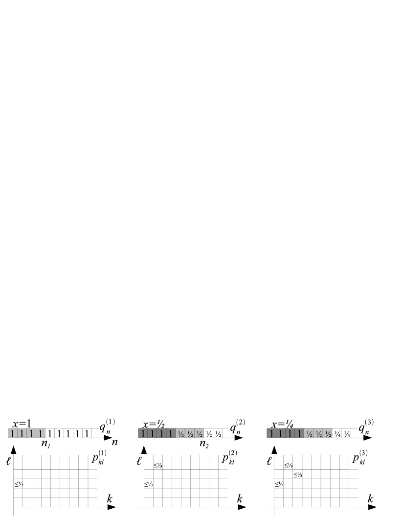
Figure 1: Illustration to the iterative construction employed in the proof of Claim 3.4

Continuing this process with $x^{(k)}:=2^{-k+1}$ for $k=3,4,\ldots$ as indicated in Figure 1 eventually yields a rational sequence $q^{(\omega)}$ with $\lim_{n}q^{(\omega)}_{n}=:x^{(\omega)}=0$, upon input of which $\mathcal{M}$ outputs a double sequence $p^{(\omega)}$ such that $p^{(\omega)}_{k,\ell_{k}}\leq\tfrac{1}{3}$ for all $k=1,2,\ldots$. In particular, $y^{(\omega)}:=\operatorname*{\smash{\sup}}\limits_{k}\operatorname*{\smash{\inf}}\limits_{\ell}p^{(\omega)}_{k,\ell}\leq\tfrac{1}{3}$ whereas $\overline{h}(x^{(\omega)})=1$ : contradiction. ∎

Notice that the above proof involves one-dimensionally indexed sequences $(q_{n})$ for input and two-dimensionally indexed ones $(p_{k,\ell})$ for output. We now proceed a step further in proof difficulty, namely involving two-dimensional indices for both input and output in order to establish Item b).

Claim 3.5

Let $f:\mathbb{R}\to\mathbb{R}$ violate monotonicity in that $f(0)=1$ and $f(1)=0$. Then, $f$ is not $(\rho_{\raisebox{0.60275pt}{${\scriptscriptstyle<}$}}^{\prime}\to\rho_{\raisebox{0.60275pt}{${\scriptscriptstyle<}$}}^{\prime})$–computable.

Proof

We construct a $\rho_{\raisebox{0.60275pt}{${\scriptscriptstyle<}$}}^{\prime}$–name for $x=0$ from an iteratively defined sequence of initial segments of $\rho_{\raisebox{0.60275pt}{${\scriptscriptstyle<}$}}^{\prime}$–names for $x=1$:

Start with $q^{(1)}_{i,j}:=1$ for all $i,j$. Then, $q^{(1)}=(q^{(1)}_{i,j})$ is obviously a $\rho_{\raisebox{0.60275pt}{${\scriptscriptstyle<}$}}^{\prime}$–name for $x=1$ and thus yields by presumption, upon input to $\mathcal{M}$, a $\rho_{\raisebox{0.60275pt}{${\scriptscriptstyle<}$}}^{\prime}$–name $p^{(1)}_{k,\ell}$ for $f(1)=0$, that is, with $0=\operatorname*{\smash{\sup}}\limits_{k}\operatorname*{\smash{\inf}}\limits_{\ell}p^{(1)}_{k,\ell}$. In particular, $p^{(1)}_{1,\ell_{1}}\leq\tfrac{1}{3}$ for some $\ell_{1}$.

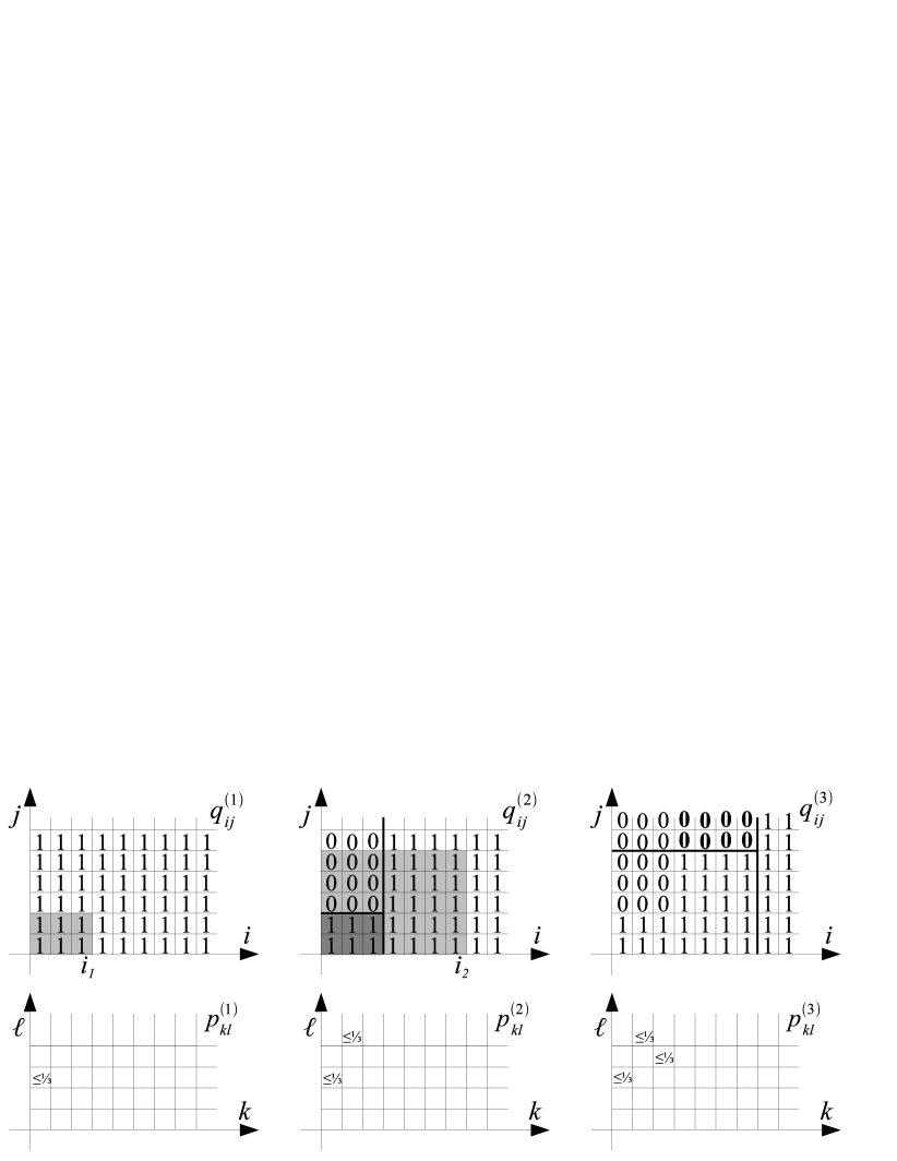
Figure 2: Illustration to the iterative construction employed in the proof of Claim 3.5

Until output of $p^{(1)}_{1,\ell_{1}}$, $\mathcal{M}$ has read only finitely many entries of $q^{(1)}$; say, up to $i_{1}$ and $j_{1}$, that is, covered in Figure 2 by the light gray rectangle. Now consider $q^{(2)}$ defined as in this figure: Since $\operatorname*{\smash{\inf}}_{j}q^{(2)}_{i,j}=0$ for $i\leq i_{1}$ and $\operatorname*{\smash{\inf}}_{j}q^{(2)}_{i,j}=1$ for $i>i_{1}$, $\operatorname*{\smash{\sup}}\limits_{i}\operatorname*{\smash{\inf}}\limits_{j}q^{(2)}_{i,j}=1$, that is, this is again valid $\rho_{\raisebox{0.60275pt}{${\scriptscriptstyle<}$}}^{\prime}$–name for $x=1$; and again, $\mathcal{M}$ will by presumption convert $q^{(2)}$ into a $\rho_{\raisebox{0.60275pt}{${\scriptscriptstyle<}$}}^{\prime}$–name $p^{(2)}$ for $f(1)=0$. In particular, $p^{(2)}_{2,\ell_{2}}\leq\tfrac{1}{3}$ for some $\ell_{2}$; and, being a deterministic machine, $\mathcal{M}$’s operation on the initial part (dark gray) on which input $q^{(2)}$ coincides with input $q^{(1)}$ will first have generated the same initial output, namely $p^{(2)}_{1,\ell_{1}}=p^{(1)}_{1,\ell_{1}}\leq\tfrac{1}{2}$.
Again, until output of $p^{(2)}_{2,\ell_{2}}$, $\mathcal{M}$ has read only a finite part of $q^{(2)}$ of, say, up to $i_{2}>i_{1}$ (light gray). By now considering input $q^{(3)}$ with $\operatorname*{\smash{\inf}}_{j}q^{(3)}_{i,j}=0$ for $i\leq i_{2}$ as in Figure 2, we arrive at $p^{(3)}$ and $\ell_{3}$ with $p^{(3)}_{1,\ell_{1}},p^{(3)}_{2,\ell_{2}},p^{(3)}_{3,\ell_{3}}\leq\tfrac{1}{3}$; and so on with $i_{3},q^{(4)},p^{(4)},\ell_{4},i_{4}$, …
Finally observe that continuing these arguments eventually leads to a rational double sequence $q^{(\omega)}=(q^{(\omega)}_{i,j})$ which has $\operatorname*{\smash{\inf}}_{j}q^{(\infty)}_{i,j}=0$ for $i\leq i_{\infty}=\infty$—and is therefore a valid $\rho_{\raisebox{0.60275pt}{${\scriptscriptstyle<}$}}^{\prime}$–name for $x=0$ (rather than $x=1$)—but gets mapped by $\mathcal{M}$ to $p^{(\omega)}=(p^{(\omega)}_{k,\ell})$ with $\operatorname*{\smash{\inf}}_{\ell}p^{(\infty)}_{k,\ell}\leq p^{(\infty)}_{k,\ell_{k}}\leq\tfrac{1}{3}$ for all $k$. Since $f(0)=1$, this contradicts our presumption that $\mathcal{M}$ maps $\rho_{\raisebox{0.60275pt}{${\scriptscriptstyle<}$}}^{\prime}$–names for $x$ to $\rho_{\raisebox{0.60275pt}{${\scriptscriptstyle<}$}}^{\prime}$–names for $f(x)$. ∎

The above proofs involving $\rho^{\prime}$ and $\rho_{\raisebox{0.60275pt}{${\scriptscriptstyle<}$}}^{\prime}$ proceeded by constructing an infinite sequence of inputs $q^{(1)},q^{(2)},\ldots,q^{(\omega)}$  (each possibly a multi-indexed sequence of its own). For finally asserting Claim c) involving $\rho^{\prime\prime}$, we will extend this method from length $\omega$, the first infinite ordinal, to an even longer one.

Claim 3.6

$\overline{h}:\mathbb{R}\to\mathbb{R}$ is not $(\rho^{\prime\prime}\to\rho^{\prime\prime})$–computable.

Proof

Outwit a Type-2 Machine $\mathcal{M}$, presumed to realize this computation, as follows:

1. Take $q^{(1)}$ to be the constant double sequence 1, i.e., $q^{(1)}_{i,j}:=1$ for all $i,j$. Being a $\rho^{\prime\prime}$–name for $1$, it is by presumption mapped to a $\rho^{\prime\prime}$–name $p^{(1)}$ for $\overline{h}(1)=0$, that is, satisfying $\lim_{k}\lim_{\ell}p^{(1)}_{k,\ell}=0$. In particular, almost every column $\#k$ contains an entry $\#\ell$ with $p^{(1)}_{k,\ell}\leq\tfrac{1}{3}$. Until output of the first such $p^{(1)}_{k_{1},\ell_{1}}$, $\mathcal{M}$ has read only a finite part of $q^{(1)}$—say, up to $i_{1},j_{1}$.

   

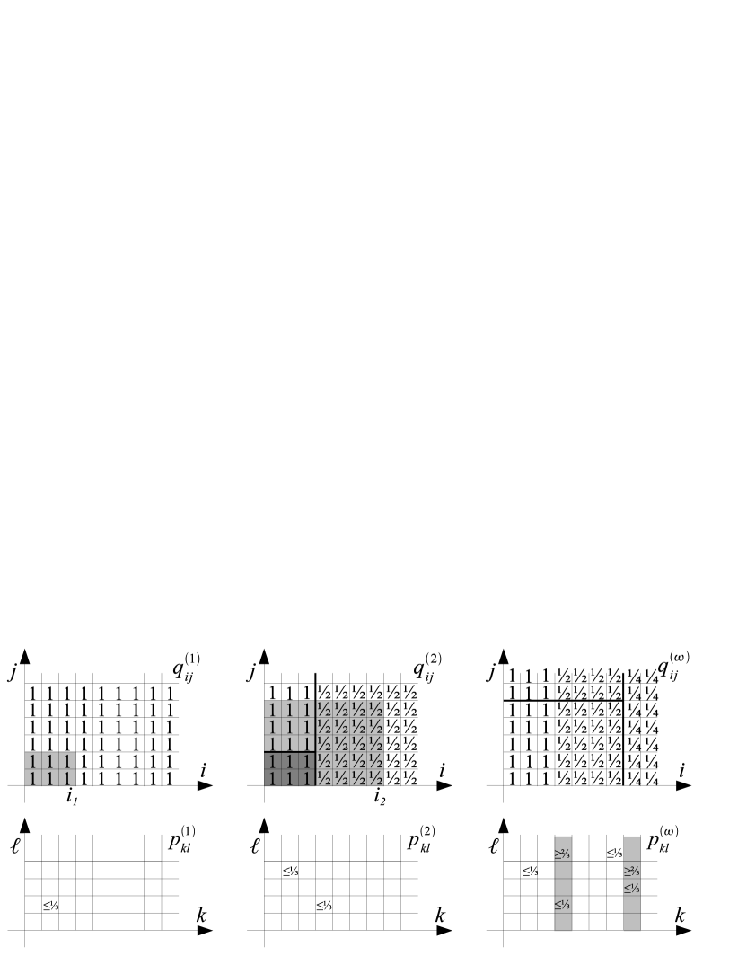
   Figure 3: The first infinitely long iterative construction employed in the proof of Claim 3.6

2. Observe that this Argument i) equally applies to the scaled input sequence $2^{-m}\cdot q^{(1)}$ for any $m$. So define $q^{(2)}_{i,j}:=q^{(1)}_{i,j}$ for $j\leq j_{1}$ (i.e., inherit the initial part of $q^{(1)}$) and $q^{(2)}_{i,j}:\equiv\tfrac{1}{2}$ for $j>j_{1}$. Now upon input of this $q^{(2)}$, $\mathcal{M}$ will output $p^{(2)}$ with, again, infinitely many $p^{(2)}_{k,\ell}\leq\tfrac{1}{3}$, the first one—$(k_{2},\ell_{2})$, say—after having read $q^{(2)}$ only up to some $(i_{2},j_{2})$. Furthermore $\mathcal{M}$’s determinism implies $p^{(2)}_{k_{1},\ell_{1}}=p^{(1)}_{k_{1},\ell_{1}}\leq\tfrac{1}{3}$.

   By repeating for $m=2,3,\ldots$, we eventually obtain—similarly to the proof of Claim 3.5—an input sequence $q^{(\omega)}$ with $q^{(\omega)}_{i,j}$ with $\lim_{i}\lim_{j}q^{(\omega)}_{i,j}=0$, that is, a valid $\rho^{\prime\prime}$–name for $x=0$ (rather than 1). This is mapped by $\mathcal{M}$ to $p^{(\omega)}$ with $p^{(\omega)}_{k_{m},\ell_{m}}\leq\tfrac{1}{3}$ for all $m$. On the other hand, $p^{(\omega)}$ is by presumption a $\rho^{\prime\prime}$–name for $\overline{h}(0)=1$. Therefore, there are infinitely many $m$ with $p^{(\omega)}_{m,\ell}\geq\tfrac{2}{3}$ for some $\ell>\ell_{m}$ and $p^{(\omega)}_{m,\ell_{m}}\leq\tfrac{1}{3}$; see the grey columns in the right part of Figure 3.

3. Since this gives no contradiction yet, we proceed by considering the first such column $m$ containing an entry $\leq\tfrac{1}{3}$ as well as an entry $\geq\tfrac{2}{3}$. Take the initial part of the input $q^{(\omega)}$ — up to $(i_{\omega},j_{\omega})$, say, depicted in grey in the left part of Figure 4 — that $\mathcal{M}$ has read until output of both of them; extend it with $\tfrac{1}{2}$s in top direction and with $1$s to the right. Feed this $\rho^{\prime\prime}$–name for $x=1$ into $\mathcal{M}$ until output of an entry $p_{k,\ell}\leq\tfrac{1}{3}$ in some column $k$ beyond $m$. Then repeat extending to the right with $1$s replaced by $\tfrac{1}{2}$s for a second entry $p_{k,\ell}\leq\tfrac{1}{3}$.

   

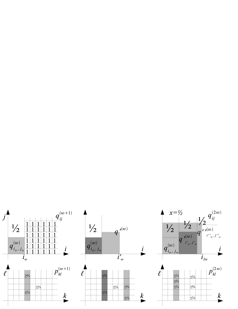
   Figure 4: Second infinitely long iterative construction employed in the proof of Claim 3.6

   More generally, proceed similarly as in ii) and extend $q^{(\omega)}_{i_{\omega},i_{\omega}}$ to the right in such a way with some $\rho^{\prime\prime}$–name $q^{\prime(\omega)}$ for $x=0$ as to obtain another column $m^{\prime}$ with both entries $\leq\tfrac{1}{3}$ and $\geq\tfrac{2}{3}$; see the middle part of Figure 4. Again, $\mathcal{M}$ outputs the latter two entries having read only a finite part; say, up to $(i^{\prime}_{\omega},j^{\prime}_{\omega})$.

   Now extend this part, too, with $\tfrac{1}{2}$ in top direction and with another $q^{\prime\prime(\omega)}$ obtained, again, as in ii) for a third column $m^{\prime\prime}$ with both entries $\leq\tfrac{1}{3}$ and $\geq\tfrac{2}{3}$; and so on.

   This eventually leads to an input $q^{(2\omega)}$ which, due to the extensions to the top, represents a $\rho^{\prime\prime}$–name for $x=\tfrac{1}{2}$ and is thus mapped by presumption to a $\rho^{\prime\prime}$–name $p^{(2\omega)}$ for $\overline{h}(\tfrac{1}{2})=0$. In particular, almost every column of $p^{(2\omega)}$ has almost every entry $\leq\tfrac{1}{3}$ while maintaining infinitely many columns with preceding entries $\leq\tfrac{1}{3}$ and $\geq\tfrac{2}{3}$; see the right part of Figure 4. This asserts the existence of infinitely many columns in $p^{(2\omega)}$ containing $\leq\tfrac{1}{3}$, $\geq\tfrac{2}{3}$, and $\leq\tfrac{1}{3}$ in order. And again, already a finite initial part of $q^{(2\omega)}$ up to some $(i_{2\omega},j_{2\omega})$ gives rise to the first such triple.

4. Notice that the arguments in iii) similarly yield the existence of an appropriate, scaled counter-part $\tfrac{1}{2}q^{\prime(2\omega)}$ of $q^{(2\omega)}$, of some $\tfrac{1}{4}q^{\prime\prime(2\omega)}$, and so on, all leading to output containing infinitely many columns with alternating triples as above. We now construct input $q^{(3\omega)}$ leading to output $p^{(3\omega)}$ containing an infinity of columns, each with four entries $\leq\tfrac{1}{3}$, $\geq\tfrac{2}{3}$, $\leq\tfrac{1}{3}$, and $\geq\tfrac{2}{3}$.

   To this end, take the initial part of $q^{(2\omega)}$ leading to output of the first column with alternating triple in the above sense; then extend it with the initial part of the scaled version $\tfrac{1}{2}q^{\prime(2\omega)}$ leading to another column with such a triple; and so on. Observing that, due to the scaling, the thus obtained $q^{(3\omega)}$ represents a $\rho^{\prime\prime}$–name for $x=0$, almost every column of the output $p^{(3\omega)}$ representing $\overline{h}(0)=1$ contains entries $\geq\tfrac{2}{3}$ in addition to the infinitely many columns with triples as above; see the left part of Figure 5.

   

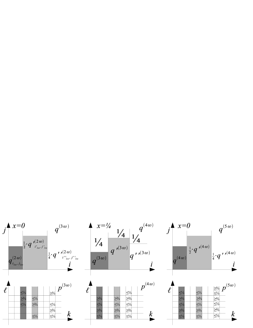
   Figure 5: Third, fourth, and fifth infinitely long iterative construction employed in the proof of Claim 3.6

5. Our next step is a $\rho^{\prime\prime}$–name $q^{(4\omega)}$ for $x=\tfrac{1}{4}$ giving rise to $p^{(4\omega)}$ with infinitely many columns containing alternating quintuples. This is obtained by repeating the arguments in iv) to obtain initial segments of (variants of) $q^{(3\omega)}$, stacking them horizontally—in order to obtain an infinity of columns with alternating quadruples—while extending in top direction with $\tfrac{1}{4}$; see the middle part of Figure 5. This forces $\mathcal{M}$ to output a $\rho^{\prime\prime}$–name $q^{(4\omega)}$ for $\overline{h}(\tfrac{1}{4})=0$ and thus with in almost every column almost every entry being $\leq\tfrac{1}{4}$, thus extending the alternating quadruples to quintuples.

6. Noticing that the vertical extension in v) was similar to step iii), we now take a step similar to iv) based on horizontally stacked initial parts of scaled counterparts of $q^{(4\omega)}$ in order to obtain a $\rho^{\prime\prime}$–name $q^{(5\omega)}$ for $x=0$ which $\mathcal{M}$ maps to some $p^{(5\omega)}$ containing infinitely many alternating six-tuples.

   Then again construct a $\rho^{\prime\prime}$–name $q^{(6\omega)}$ for $x=\tfrac{1}{8}$ by horizontally stacking initial segments of (variants of) $q^{(5\omega)}$ while extending them vertically with $\tfrac{1}{8}$ and so on.

Now for the bottom line: By proceeding the above construction, one eventually obtains a rational double sequence $q^{(\omega^{2})}$ with $\lim_{j}q^{(\omega^{2})}_{i,j}=0$ for all $i$ — that is, a $\rho^{\prime\prime}$–name for $x=0$ — mapped by $\mathcal{M}$ to some $p^{(\omega^{2})}$ containing (infinitely many) columns $\#k$ with infinitely many alternating entries $\leq\tfrac{1}{3}$ and $\geq\tfrac{2}{3}$ — contradicting that, for $\rho^{\prime\prime}$-names $p=(p_{k,\ell})$, $\lim_{\ell}p_{k,\ell}$ is required to exist for every $k$. ∎

4 Hierarchies of Hypercomputable Real Functions

The present section investigates and compares the first levels of the two hierarchies of hypercomputable real functions induced by the two approaches to real function hypercomputation considered in Section 3: based on oracle support and based on weakened encodings.

4.1 Weakly Computable Real Functions

For every $(\alpha\to\beta)$–computable function $f:A\to B$, one may obviously replace representation $\alpha$ for $A$ by a stronger one and $\beta$ for $B$ by a weaker one while maintaining computability of $f$:
$\displaystyle f\quad(\alpha\to\beta)\text{--computable}\;\wedge\;\;\alpha,\preceq\alpha\;\;\wedge\;\beta\preceq\beta^{\prime}\quad\Rightarrow\quad f\quad(\alpha,\to\beta^{\prime})\text{--computable}$.
However if both $\alpha$ and $\beta$ are made, say, weaker then $(\alpha^{\prime}\to\beta^{\prime})$–computability of $f$ may in general be violated. For $\alpha=\beta=\rho_{\raisebox{0.60275pt}{${\scriptscriptstyle<}$}}$, though, we have seen in Example 1 that the implication “$(\rho_{\raisebox{0.60275pt}{${\scriptscriptstyle<}$}}\to\rho_{\raisebox{0.60275pt}{${\scriptscriptstyle<}$}})\Rightarrow(\rho_{\raisebox{0.60275pt}{${\scriptscriptstyle<}$}}^{\prime}\to\rho_{\raisebox{0.60275pt}{${\scriptscriptstyle<}$}}^{\prime})$” does hold at least for the case of $f$ being Heaviside’s function. By the following result, it holds in fact for every $f$:

Theorem 4.1 (Second Main Theorem of Real Hypercomputation)

Consider $f:\mathbb{R}\to\mathbb{R}$.

1. If $f$ is $(\rho\to\rho)$–computable, then it is also $(\rho^{\prime}\to\rho^{\prime})$–computable.

2. If $f$ is $(\rho\to\rho_{\raisebox{0.60275pt}{${\scriptscriptstyle<}$}})$–computable, then it is also $(\rho^{\prime}\to\rho_{\raisebox{0.60275pt}{${\scriptscriptstyle<}$}}^{\prime})$–computable.

3. If $f$ is $(\rho_{\raisebox{0.60275pt}{${\scriptscriptstyle<}$}}\to\rho_{\raisebox{0.60275pt}{${\scriptscriptstyle<}$}})$–computable, then it is also $(\rho_{\raisebox{0.60275pt}{${\scriptscriptstyle<}$}}^{\prime}\to\rho_{\raisebox{0.60275pt}{${\scriptscriptstyle<}$}}^{\prime})$–computable.

4. If $f$ is $(\rho^{\prime}\to\rho^{\prime})$–computable, then it is also $(\rho^{\prime\prime}\to\rho^{\prime\prime})$–computable.

5. If $f$ is $(\rho^{\prime\prime}\to\rho^{\prime\prime})$–computable, then it is also $(\rho^{\prime\prime\prime}\to\rho^{\prime\prime\prime})$–computable.

The claims remain valid under oracle-supported computation.

As a consequence, we obtain the following partial strengthening of Lemma 1:

Corollary 1

It holds   $\displaystyle\rho\;\>\equiv\;\>\,\rho_{\raisebox{0.60275pt}{${\scriptscriptstyle<}$}}\!\wedge\rho_{\raisebox{0.60275pt}{${\scriptscriptstyle>}$}}\;\>{}_{\text{t}}\;\>\rho_{\raisebox{0.60275pt}{${\scriptscriptstyle<}$}}\;\>{}_{\text{t}}\;\rho^{\prime}\;\>\equiv\;\>\,\rho_{\raisebox{0.60275pt}{${\scriptscriptstyle<}$}}^{\prime}\!\wedge\rho_{\raisebox{0.60275pt}{${\scriptscriptstyle>}$}}^{\prime}\;\>{}_{\text{t}}\;\>\rho_{\raisebox{0.60275pt}{${\scriptscriptstyle<}$}}^{\prime}\;\>{}_{\text{t}}\;\>\rho^{\prime\prime}$
where “ $\preceq_{\text{t}}\!$” denotes continuous reducibility of representations [Wei01, Def. 2.3.2].

Proof

The positive claims follow from Lemmas 1 and 2. For a negative claim like “$\rho_{\raisebox{0.60275pt}{${\scriptscriptstyle<}$}}^{\prime}\npreceq_{\text{t}}\rho^{\prime}$” suppose the contrary. Then by Lemma 2, with the help of some appropriate oracle $\mathcal{O}$, one can convert $\rho_{\raisebox{0.60275pt}{${\scriptscriptstyle<}$}}^{\prime}$–names to $\rho^{\prime}$–names. As Heaviside’s function $h$ is $(\rho^{\prime}\to\rho_{\raisebox{0.60275pt}{${\scriptscriptstyle<}$}}^{\prime})$–computable by Example 1 and Theorem 4.1, composition with the presumed conversion implies $(\rho^{\prime}\to\rho^{\prime})$–computability of $h$ relative to $\mathcal{O}$—contradicting Theorem 3.3c). ∎

Proof (Theorem 4.1d)

Let $f$ be $(\rho^{\prime}\to\rho^{\prime})$–computable and $x$ given by a $\rho^{\prime\prime}$–name, that is, a rational sequence $q=(q_{n})$ with $x=\lim_{i}\lim_{j}q_{\scriptscriptstyle\langle i,j\rangle}$. For each $i$, compute by assumption from the $\rho^{\prime}$–name $q_{\scriptscriptstyle\langle i,\cdot\rangle}=(q_{\scriptscriptstyle\langle i,j\rangle})_{{}_{j}}$ of $x_{i}:=\lim_{j}q_{\scriptscriptstyle\langle i,j\rangle}$ a $\rho^{\prime}$–name of $f(x_{i})$, that is, a sequence $p=p_{\scriptscriptstyle\langle i,\cdot\rangle}=(p_{\scriptscriptstyle\langle i,j\rangle})_{{}_{j}}$ with $f(x_{i})=\lim_{j}p_{\scriptscriptstyle\langle i,j\rangle}$. Continuity of $f$ due to Fact 3.2c) asserts

$$\lim_{i}\lim_{j}p_{\scriptscriptstyle\langle i,j\rangle}\;=\;\lim_{i}f(x_{i})\;\overset{!}{=}\;f\big{(}\lim_{i}x_{i}\big{)}\;=\;f\big{(}\lim_{i}\lim_{j}q_{\scriptscriptstyle\langle i,j\rangle}\big{)}\;=\;f(x)$$

this sequence $p$ to be a $\rho^{\prime\prime}$–name for $y=f(x)$. ∎

Where the last proof exploited Fact 3.2c), the next one relies on Theorem 3.3c):

Proof (Theorem 4.1e)

A $\rho^{\prime\prime\prime}$–name for $x\in\mathbb{R}$ is a rational sequence $a=(q_{n})$ with $x=\lim_{i}\lim_{j}\lim_{k}q_{\scriptscriptstyle\langle i,j,k\rangle}$. For each $i$, exploit $(\rho^{\prime\prime}\to\rho^{\prime\prime})$–computability of $f$ to obtain, from the $\rho^{\prime\prime}$–name $q_{\scriptscriptstyle\langle i,\,\cdot\,,\,\cdot\,\rangle}$ of $x_{i}:=\lim_{j}\lim_{k}q_{\scriptscriptstyle\langle i,j,k\rangle}\in\mathbb{R}$, a sequence $p_{\scriptscriptstyle\langle i,\,\cdot\,,\,\cdot\,\rangle}$ with $\lim_{j}\lim_{k}p_{\scriptscriptstyle\langle i,j,k\rangle}$ as $\rho^{\prime\prime}$–name of $f(x_{i})$. Similarly to case d), this sequence $p$ constitutes a $\rho^{\prime\prime\prime}$–name for $y=f(x)$ by continuity of $f$ due to Theorem 3.3c). ∎

Proof (Theorem 4.1a)

Let $f$ be $(\rho\to\rho)$–computable. Its $(\rho^{\prime}\to\rho^{\prime})$–computability is established as follows: Given $(q_{n})\subseteq\mathbb{Q}$ with $x=\lim_{n}q_{n}$, apply the assumption to evaluate $f(q_{n})$ for each $n$ up to error $2^{-n}$; that is, obtain $p_{n}\in\mathbb{Q}$ with $|p_{n}-f(q_{n})|\leq 2^{-n}$. Since $f$ is continuous by Fact 3.2a), it follows $f(x)=\lim_{n}f(q_{n})=\lim_{n}p_{n}$ so that $(p_{n})$ is a $\rho^{\prime}$–name for $y=f(x)$. ∎

It is interesting that the latter proof works in fact uniformly in $f$, i.e., we have

Scholium 4.2

The apply operator  $C(\mathbb{R})\times\mathbb{R}\ni(f,x)\mapsto f(x)$  is $([\rho\!\to\!\rho]\times\rho^{\prime}\to\rho^{\prime})$–computable.

Similarly, Theorem 4.1b) follows from Lemma 3 below together with the observation that every $(\rho\to\rho_{\raisebox{0.60275pt}{${\scriptscriptstyle<}$}})$–computable $f$ has a computable $[\rho\!\to\!\rho_{\raisebox{0.60275pt}{${\scriptscriptstyle<}$}}]$–name [WZ00, Corollary 5.1(2) and Theorem 3.7]; here, $[\rho\!\to\!\rho_{\raisebox{0.60275pt}{${\scriptscriptstyle<}$}}]$ denotes a natural representation for the space $\operatorname{LSC}(\mathbb{R})$ of lower semi-continuous functions $f:\mathbb{R}\to\mathbb{R}$ considered in [WZ00]. Specifically, a $[\rho\!\to\!\rho_{\raisebox{0.60275pt}{${\scriptscriptstyle<}$}}]$–name for such a $f$ is an enumeration of all rational triples $(a,b,c)$ such that $c<\min f\big{[}[a,b]\big{]}$—the latter making sense as a lower semi-continuous function attains its minimum (though not necessarily its maximum) on any compact set. $[\rho\!\to\!\rho_{\raisebox{0.60275pt}{${\scriptscriptstyle<}$}}]$ indeed is a representation for $\operatorname{LSC}(\mathbb{R})$ because different lower semi-continuous functions give rise to different such collections $\{(a,b,c)\in\mathbb{Q}^{3}:\ldots\}$; cf. [WZ00, Lemma 3.3].

Lemma 3

$\operatorname{LSC}(\mathbb{R})\times\mathbb{R}\ni(f,x)\mapsto f(x)$  is  $([\rho\!\to\!\rho_{\raisebox{0.60275pt}{${\scriptscriptstyle<}$}}]\times\rho^{\prime}\to\rho_{\raisebox{0.60275pt}{${\scriptscriptstyle<}$}}^{\prime})$–computable.

Proof

Let $(a_{k},b_{k},c_{k})_{{}_{k}}$ denote the given $[\rho\!\to\!\rho_{\raisebox{0.60275pt}{${\scriptscriptstyle<}$}}]$–name of $f\in\operatorname{LSC}(\mathbb{R})$ and $(q_{n})_{{}_{n}}$ the given $\rho^{\prime}$–name for $x\in\mathbb{R}$. Our goal is to $\rho_{\raisebox{0.60275pt}{${\scriptscriptstyle<}$}}^{\prime}$–compute $y:=f(x)$. Define the sequence $p=(p_{m})_{{}_{m}}\subseteq\mathbb{Q}\cup\{+\infty\}$ by

$$p_{{}_{\langle k,\ell,n\rangle}}\;:=\;\left\{\begin{array}[]{ll}\max\big{\{}c_{m}\;:\;m\leq k\;\wedge&[a_{m},b_{m}]\supseteq[a_{k},b_{k}]\big{\}}\\[0.86108pt] &\text{ if }q_{n}\in(a_{k},b_{k})\;\wedge\;|b_{k}-a_{k}|=2^{-\ell}\\[2.15277pt] +\infty&\text{ otherwise}\end{array}\right.$$ (1)

From the given information, one can obviously compute $p$. Moreover this sequence satisfies

• $\liminf p\geq y$:
  Let $\epsilon>0$ be arbitrary. Since $f$ is lower semi-continuous, its preimage $f^{-1}\big{[}(y-\epsilon,\infty)\big{]}\ni x$ is an open set and therefore contains an entire ball around $x$. In fact, the center of this ball may be chosen as rational and its diameter of the form $2^{-L}$ for some $L\in\mathbb{N}$; formally (see Figure 6):

  $$\exists K,L,K^{\prime}\in\mathbb{N}:\quad x\in(a_{K^{\prime}},b_{K^{\prime}})\subseteq[a_{K},b_{K}]\subseteq f^{-1}\big{[}(y-\epsilon,\infty)\big{]}\;\;\wedge\\ |b_{K}-a_{K}|=2^{-L}\;\wedge\;a_{K^{\prime}}=a_{K}+\tfrac{3}{2}\cdot 2^{-L-2}\;\wedge\;b_{K^{\prime}}=b_{K}-\tfrac{3}{2}\cdot 2^{-L-2}$$ (2)

  where we have exploited that every rational pair $(a,b)$ occurs in the list representing the $[\rho\!\to\!\rho_{\raisebox{0.60275pt}{${\scriptscriptstyle<}$}}]$–name. Moreover, as it consists of all rational triples $(a,b,c)$ with $c<\min f\big{[}[a,b]\big{]}$,

  $$\exists M\geq K:\;\;[a_{K},b_{K}]=[a_{M},b_{M}]\;\wedge\;c_{M}\geq\min f\big{[}[a_{M},b_{M}]\big{]}-\epsilon\overset{\text{(*)}}{\;\geq\;}y-2\epsilon$$ (3)

  with (*) a consequence of $[a_{K},b_{K}]\subseteq f^{-1}\big{[}(y-\epsilon,\infty)\big{]}$ in Equation (2). Finally,

  $$\lim_{n}q_{n}=x\in(a_{K^{\prime}},b_{K^{\prime}})\qquad\Rightarrow\quad\exists N:\;\forall n\geq N:\;\;q_{n}\in(a_{K^{\prime}},b_{K^{\prime}})\enspace.$$ (4)

  So putting things together, for each $n\geq N$, $\ell\geq L^{\prime}$, and $k\geq M$, we either have $p_{{}_{\langle k,\ell,n\rangle}}=+\infty\geq y-2\epsilon$; or we are in the first case of Equation (1), thus

  • $q_{n}\in(a_{k},b_{k})$ with $|b_{k}-a_{k}|\leq 2^{-\ell}$

  • $q_{n}\in(a_{K^{\prime}},b_{K^{\prime}})$ by Equation (4)

  • hence $[a_{k},b_{k}]\subseteq[a_{K},b_{K}]$ by Equation (2) due to $\ell\geq L^{\prime}$; cf. Figure 6.

  • So $[a_{k},b_{k}]\subseteq[a_{M},b_{M}]$ by Equation (3)

  • implying $p_{{}_{\langle k,\ell,n\rangle}}\geq c_{M}\geq y-2\epsilon$ by Equations (1) and (3) since $k\geq M$.

  Summarizing, it holds $p_{{}_{\langle k,\ell,n\rangle}}\geq y-2\epsilon$ for all $(k,\ell,n)\in\mathbb{N}^{3}$ not belonging to the finite set $\{0,1,\ldots,N-1\}\times\{0,1,\ldots,L^{\prime}-1\}\times\{0,1,\ldots,M-1\}$ of exceptions. Consequently $\liminf p\geq y-2\epsilon$; even $\liminf p\geq y$ because $\epsilon>0$ was arbitrary.

  

  Figure 6: Nesting of some rational intervals of dyadic length contained in $f^{-1}\big{[}(y-\epsilon,\infty)\big{]}$.
  The parameters are chosen in such a way that, whenever $(a_{K^{\prime}},b_{K^{\prime}})$ meets some other $(a_{k},b_{k})$ of length $|b_{k}-a_{k}|=2^{-\ell}$ for $\ell\geq L^{\prime}:=L+2$, then $[a_{k},b_{k}]$ is entirely contained within the larger $[a_{K},b_{K}]$.

• $\liminf p\leq y$
  Indeed: Since the $[\rho\!\to\!\rho_{\raisebox{0.60275pt}{${\scriptscriptstyle<}$}}]$–name contains in particular all rational pairs $(a_{k},b_{k})$ and these intervals are dense in $\mathbb{R}$, there exists to every $\ell\in\mathbb{N}$ some $k$ such that $|b_{k}-a_{k}|=2^{-\ell}$ and $x\in(a_{k},b_{k})$. Furthermore it holds $q_{n}\in(a_{k},b_{k})$ for some sufficiently large $n$ because $\lim_{n}q_{n}=x$. We have thus infinitely many triples $(k,\ell,n)$ for which $p_{{}_{\langle k,\ell,n\rangle}}$ is defined by the first case in Equation (1) and thus agrees with some $c_{m}<\min f\big{[}[a_{m},b_{m}]\big{]}\leq f(x)=y$ as $x\in(a_{k},b_{k})\subseteq[a_{m},b_{m}]$.

Concluding, we have $\liminf_{m}p_{m}=y$. Although $p$ may attain the value $+\infty$, this can easily be overcome by proceeding to $\tilde{p}_{m}:=p_{m}$ for $p_{m}\not=\infty$ and $\tilde{p}_{m}:=\max\{0,\tilde{p}_{0},\ldots,\tilde{p}_{m-1}\}$ for $p_{m}=\infty$ because this transformation $p\mapsto\tilde{p}$ on sequences obviously does not affect their $\liminf<\infty$. This yields a $\tilde{\rho}_{\raisebox{0.60275pt}{${\scriptscriptstyle<}$}}^{\prime}$–name for $y$ which can finally be converted to the desired $\rho_{\raisebox{0.60275pt}{${\scriptscriptstyle<}$}}^{\prime}$–name due to the easy part of Scholium 2.2. ∎

In order to obtain a similar uniform claim yielding Theorem 4.1c), recall that every $(\rho_{\raisebox{0.60275pt}{${\scriptscriptstyle<}$}}\to\rho_{\raisebox{0.60275pt}{${\scriptscriptstyle<}$}})$–computable function $f:\mathbb{R}\to\mathbb{R}$ is necessarily both monotonically increasing and lower semi-continuous (Fact 3.2b+c). This suggests

Definition 3

Let $\operatorname{MLSC}(\mathbb{R})$ denote the class of all monotonically increasing, lower semi-continuous functions $f:\mathbb{R}\to\mathbb{R}$. A $[\rho_{\raisebox{0.60275pt}{${\scriptscriptstyle<}$}}\!\to\!\rho_{\raisebox{0.60275pt}{${\scriptscriptstyle<}$}}]$–name for $f\in\operatorname{MLSC}(\mathbb{R})$ is an enumeration of the set $\{(a,c)\in\mathbb{Q}^{2}:c<f(a)\}$.

Lemma 4

1. Distinct $f,g\in\operatorname{MLSC}(\mathbb{R})$ have different sets $\{(a,c):\ldots\}$ according to Definition 3; that is, $[\rho_{\raisebox{0.60275pt}{${\scriptscriptstyle<}$}}\!\to\!\rho_{\raisebox{0.60275pt}{${\scriptscriptstyle<}$}}]$ constitutes a well-defined representation.

2. A function $f\in\operatorname{MLSC}(\mathbb{R})$ is $(\rho_{\raisebox{0.60275pt}{${\scriptscriptstyle<}$}}\to\rho_{\raisebox{0.60275pt}{${\scriptscriptstyle<}$}})$–computable iff it has a computable $[\rho_{\raisebox{0.60275pt}{${\scriptscriptstyle<}$}}\!\to\!\rho_{\raisebox{0.60275pt}{${\scriptscriptstyle<}$}}]$–name.

3. Let $f\in\operatorname{MLSC}(\mathbb{R})$, $(a_{k},c_{k})_{{}_{k}}$ with $\{(a,c)\in\mathbb{Q}^{2}:c<f(a)\}=\{(a_{k},c_{k}):k\in\mathbb{N}\}$, $x\in\mathbb{R}$, and $q=(q_{n})\subseteq\mathbb{Q}$ with $x=\liminf_{n}q_{n}$. Then, the rational sequence $p$ defined by

   $$p_{{}_{\langle k,n,\ell\rangle}}\;:=\;\left\{\begin{array}[]{ll}\max\big{\{}c_{m}\;:\;m\leq k\;\wedge\;a_{m}\geq a_{k}\big{\}}&\text{ ~{}if~{} }a_{k}<q_{n}<a_{k}+2^{-\ell}\\[2.15277pt] +\infty&\text{ ~{}otherwise}\end{array}\right.$$

   satisfies  $\liminf p=f(x)=:y$.

4. Therefore, the apply operator  $\operatorname{MLSC}(\mathbb{R})\times\mathbb{R}\;\ni\;(f,x)\;\mapsto\;f(x)$  is  $([\rho_{\raisebox{0.60275pt}{${\scriptscriptstyle<}$}}\!\to\!\rho_{\raisebox{0.60275pt}{${\scriptscriptstyle<}$}}]\times\rho_{\raisebox{0.60275pt}{${\scriptscriptstyle<}$}}^{\prime}\to\rho_{\raisebox{0.60275pt}{${\scriptscriptstyle<}$}}^{\prime})$–computable.

Proof

1. Let $f,g\in\operatorname{MLSC}(\mathbb{R})$ with $f\not=g$, that is, w.l.o.g. $f(x_{0})<g(x_{0})$ for some $x_{0}\in\mathbb{R}$. There exists some $c_{0}\in\mathbb{Q}$ with $f(x_{0})<c_{0}<g(x_{0})$. Being monotonically increasing and lower semi-continuous, their pre-images $f^{-1}\big{[}(c_{0},\infty)\big{]}\not\ni x_{0}$ and $g^{-1}\big{[}(c_{0},\infty)\big{]}\ni x_{0}$ on open half-interval $(c_{0},\infty)$ are again open half-intervals $(x_{f},\infty)$ and $(x_{g},\infty)$, respectively. As $x_{0}$ belongs to the second but not to the first, we have $x_{g}<x_{0}<x_{f}$ and therefore $x_{g}<a_{0}<x_{f}$ for some $a_{0}\in\mathbb{Q}$. Then $a_{0}\in(x_{g},\infty)=g^{-1}\big{[}(c_{0},\infty)\big{]}$ yields $c_{0}<g(a_{0})$ whereas $a_{0}\not\in(x_{f},\infty)=f^{-1}\big{[}(c_{0},\infty)\big{]}$ asserts $c_{0}\not<f(a_{0})$.

2. Let $\mathcal{M}$ denote a Type-2 Machine $(\rho_{\raisebox{0.60275pt}{${\scriptscriptstyle<}$}}\to\rho_{\raisebox{0.60275pt}{${\scriptscriptstyle<}$}})$–computing $f\in\operatorname{MLSC}(\mathbb{R})$. Evaluating $f$ at $a\in\mathbb{Q}$ by simulating $\mathcal{M}$ on the $\rho_{\raisebox{0.60275pt}{${\scriptscriptstyle<}$}}$–name $(a,a,a,\ldots)$ for $a$ thus yields a $\rho_{\raisebox{0.60275pt}{${\scriptscriptstyle<}$}}$–name for $f(a)$ which is (equivalent to) a list of all $c\in\mathbb{Q}$ with $c<f(a)$ [Wei01, Lemma 4.1.8]. So dove-tailing this simulation for all $a\in\mathbb{Q}$ yields the desired $[\rho_{\raisebox{0.60275pt}{${\scriptscriptstyle<}$}}\!\to\!\rho_{\raisebox{0.60275pt}{${\scriptscriptstyle<}$}}]$–name for $f$.

   Conversely, knowing a $[\rho_{\raisebox{0.60275pt}{${\scriptscriptstyle<}$}}\!\to\!\rho_{\raisebox{0.60275pt}{${\scriptscriptstyle<}$}}]$–name $(a_{k},c_{k})_{{}_{k}}$ for $f\in\operatorname{MLSC}(\mathbb{R})$ and given an increasing sequence $(q_{n})\subseteq\mathbb{Q}$ with $x=\sup_{n}q_{n}$, let

   $$p_{n}:=c_{n}\text{ ~{}if~{} }a_{n}\leq q_{n},\qquad p_{n}:=-\infty\text{ ~{}otherwise}\enspace.$$

   Then, in the first case, $p_{n}=c_{n}<f(a_{n})\leq f(q_{n})\leq f(x)=:y$ by monotonicity, and $p_{n}=-\infty\leq y$ in the second; hence $\sup_{n}p_{n}\leq y$. To see $\sup_{n}p_{n}\geq y$, fix arbitrary $\epsilon>0$ and consider the open half-interval $f^{-1}\big{[}(y-\epsilon,\infty)\big{]}=(x_{\epsilon},\infty)$ containing $x$ and thus also some rational $a=a_{K}\in(x_{\epsilon},x)$, $K\in\mathbb{N}$. Furthermore $q_{n}\nearrow x$ yields some $N\in\mathbb{N}$ such that $q_{n}\in(a_{K},x)$ for all $n\geq N$. And finally there exists $M\geq N$ with $a_{M}=a_{K}$ and $c_{M}\geq f(a_{M})-\epsilon$. Together this asserts $q_{M}>a_{K}=a_{M}$ because $M\geq N$ and thus $p_{M}=c_{M}\geq f(a_{K})-\epsilon>y-2\epsilon$ due to $a_{k}\in f^{-1}\big{[}(y-\epsilon,\infty)\big{]}$.

3. Take arbitrary $\epsilon>0$. As $f$ is increasing and lower semi-continuous, the pre-image $f^{-1}\big{[}(y-\epsilon,\infty)\big{]}$ is an open half-interval $(x_{\epsilon},\infty)$ containing $x$. Therefore there exist $K,L\in\mathbb{N}$ such that $x_{\epsilon}<a_{K}$ and $a_{K}+2^{-L}<x$; furthermore, the sequence $(a_{k},c_{k})_{{}_{k}}$ containing all rational pairs $(a,c)$ with $c<f(a)$, there is $M\geq K$ such that $a_{M}=a_{K}$ and $c_{M}\geq f(a_{M})-\epsilon$; and finally, since $\liminf_{n}q_{n}=x>a_{M}+2^{-L}$, it holds $q_{n}>a_{M}+2^{-L}$ for all $n\geq N$ with an appropriate $N\in\mathbb{N}$. Observe that $q>a_{M}+2^{-L}$ and $a<q<a+2^{-L}$ implies $a\geq a_{M}$; so together we have for all $n\geq N$, $\ell\geq L$, and $k\geq M$ that $p_{{}_{\langle k,n,\ell\rangle}}$ is either $+\infty$ or $\geq c_{M}\geq f(a_{K})-\epsilon\geq f(x_{\epsilon})-\epsilon\geq y-2\epsilon$ due to monotonicity of $f$ and by definition of $x_{\epsilon}<a_{K}$. This proves $\liminf p\geq y$ because $\epsilon$ was arbitrary.

   To see the reverse inequality “$\liminf p\leq y$”, take arbitrary $\ell\in\mathbb{N}$. There exists $k\in\mathbb{N}$ with $a_{k}<x<a_{k}+2^{-\ell}$ and, because of $\liminf_{n}q_{n}=x$, also $n\in\mathbb{N}$ with $a_{k}<q_{n}<a_{k}+2^{-\ell}$. We therefore have infinitely many triples $(n,k,\ell)$ for which $p_{{}_{\langle n,k,\ell\rangle}}$ agrees with a certain $c_{m}<f(a_{m})\leq f(a_{k})\leq f(x)=y$.

4. Given a $\rho_{\raisebox{0.60275pt}{${\scriptscriptstyle<}$}}^{\prime}$–name for $x$, one can obtain a sequence $(q_{n})\subseteq\mathbb{Q}$ with $x=\liminf_{n}q_{n}$ by virtue of Scholium 2.2. From this, the sequence $p\subseteq\mathbb{Q}$ with $\liminf p=f(x)$ according to c) is obviously computable and yields, again by Scholium 2.2, a $\rho_{\raisebox{0.60275pt}{${\scriptscriptstyle<}$}}^{\prime}$–name for $y=f(x)$. ∎

Concluding this subsection, the classes of $(\rho^{(d)}\to\rho^{(d)})$–computable real functions $f:\mathbb{R}\to\mathbb{R}$ form, for $d=0,1,\ldots$ respectively, a hierarchy. By Fact 2.1, this hierarchy is strict as can be seen from the constant functions $f(x)\equiv c$ with $c\in\Delta_{d+1}\mathbb{R}$.

4.2 Arithmetic Weierstraß Hierarchy

Section 4.1 established the sequence  $\rho,\rho^{\prime},\rho^{\prime\prime},\ldots$  of increasingly weaker representations for $\mathbb{R}$ to yield the strict hierarchy of $(\rho\to\rho)$–computable, $(\rho^{\prime}\to\rho^{\prime})$–computable, and $(\rho^{\prime\prime}\to\rho^{\prime\prime})$–computable functions $f:[0,1]\to\mathbb{R}$. We now compare these classes with those induced by the other kind of real hypercomputation suggested in Section 3: relative to the Halting Problem $H=\emptyset^{\prime}$ and its iterated jumps $\emptyset^{\prime\prime}$, …

Such a comparison makes sense because both weakly and oracle-computable real functions are necessarily continuous according to Fact 3.2d)/Theorem 3.3c) and Lemma 2, respectively.

The classical Weierstraß Approximation Theorem establishes any continuous real function $f:[0,1]\to\mathbb{R}$ to be the uniform limit $f=\operatorname*{ulim}_{n}P_{n}$ of a sequence of rational polynomials $(P_{n})\subseteq\mathbb{Q}[X]$. Here, ‘$\operatorname*{ulim}$’ suggestively denotes uniform convergence of continuous functions on $[0,1]$, that is the requirement

$$\sup\limits_{0\leq x\leq 1}|f(x)-P_{n}(x)|\;\;=:\;\;\|f-P_{n}\|\;\to\;0\qquad\text{as~{} }n\to\infty\enspace.$$

The famous Effective Weierstraß Theorem due to Pour-El, Caldwell, and Hauck relates effectively evaluable to effectively approximable real functions:

Fact 4.3

A function $f:[0,1]\to\mathbb{R}$ is $(\rho\to\rho)$–computable if and only if it holds
 $\boldsymbol{[\rho\!\to\!\rho]}$: There exists a computable sequence of  (degrees and coefficients of) rational polynomials $(P_{n})\subseteq\mathbb{Q}[X]$ such that $$\|f-P_{n}\|\;\leq\;2^{-n}$$ (5)

Proof

See [PER89, Section 0.7], [PEC75], or [Hau76].
The notion “$[\rho\!\to\!\rho]$” is justified as the list $(P_{n})_{{}_{n}}$ constitutes (or is equivalent to) a $[\rho\!\to\!\rho]$–name for $f=\operatorname*{ulim}_{n}P_{n}$; cf. [Wei01, bottom of p.160].∎

The aforementioned other approach to continuous real hypercomputation arises from allowing the fast convergent sequence $(P_{n})_{{}_{n}}\subseteq\mathbb{Q}[X]$ to be computable in $\emptyset^{\prime}$ or $\emptyset^{\prime\prime}$. The $\emptyset^{\prime}$–computable $f:[0,1]\to\mathbb{R}$ have in fact already been characterized by Ho as Claim a) of the following

Lemma 5

1. To a real function $f:[0,1]\to\mathbb{R}$, there exists a $\emptyset^{\prime}$–computable sequence of polynomials $(P_{n})$ satisfying Equation (5)  if and only if  it holds
   $\boldsymbol{[\rho\!\to\!\rho]^{\prime}}$: There is a computable sequence $(Q_{m})\subseteq\mathbb{Q}[X]$ converging uniformly (although not necessarily ‘fast’) to $f$, that is, with $f=\operatorname*{ulim}\limits_{m\to\infty}Q_{m}$.

2. For an arbitrary oracle $A$, the sequence (of discrete degrees and numerators/denominators of the coefficients of)  $(P_{n})_{{}_{n}}\subseteq\mathbb{Q}[X]$  is $A^{\prime}$–computable  iff  there exists an $A$–computable sequence  $(Q_{n,m})_{{}_{n,m}}\subseteq\mathbb{Q}[X]$  such that

   $$\forall n\;\exists M\;\forall m\geq M:\quad P_{n}=Q_{n,m}\enspace.$$

3. To a real function $f:[0,1]\to\mathbb{R}$, there exists a $\emptyset^{\prime\prime}$–computable sequence of polynomials $(P_{n})$ satisfying Equation (5)  if and only if  it holds
   $\boldsymbol{[\rho\!\to\!\rho]^{\prime\prime}}$: There is a computable sequence $(Q_{m})\subseteq\mathbb{Q}[X]$ s.t. $f=\operatorname*{ulim}\limits_{i}\operatorname*{ulim}\limits_{j}Q_{\scriptscriptstyle\langle i,j\rangle}$.

Notice the similarity of Claims a+c) to Fact 2.1b).

Proof

1. See [Ho99, Theorem 16].

2. is a straight-forward extension of Shoenfield’s Limit Lemma [Soa87, Lemma III.3.3] and its generalization to sequences of rational numbers [ZW01, Lemma 4.1].

3. If $\emptyset^{\prime\prime}$–computable  $(P_{n})_{{}_{n}}\subseteq\mathbb{Q}[X]$  satisfies Equation (5), then by virtue of the relativization of [Ho99, Theorem 16] there exists some $\emptyset^{\prime}$–computable  $(\tilde{P}_{n})_{{}_{n}}\subseteq\mathbb{Q}[X]$  converging to the same $f$ uniformly on $[0,1]$. By Claim a) in turn, $\tilde{P}_{n}=\operatorname*{ulim}_{m}Q_{n,m}$ for some computable sequence $(Q_{n,m})\subseteq\mathbb{Q}[X]$.

   Conversely if $f=\operatorname*{ulim}_{n}\tilde{P}_{n}$ with $\tilde{P}_{n}:=\operatorname*{ulim}_{m}Q_{n,m}$ for a computable $(Q_{n,m})$, then let $P_{n}:=Q_{n,m_{n}}$ where

   $$m_{n}\quad:=\quad\min\big{\{}m\in\mathbb{N}\>\big{|}\,\forall k,\ell\geq m\,:\,\|Q_{n,k}-Q_{n,\ell}\|\leq 2^{-n}\big{\}}\enspace.$$ (6)

   This sequence $(m_{n})_{{}_{n}}$ is well-defined and yields  $\|P_{n}-\tilde{P}_{n}\|\leq 2^{-n}$, so $f=\operatorname*{ulim}_{n}\tilde{P}_{n}=\operatorname*{ulim}_{n}P_{n}$. Moreover, the minimum in Equation (6) is taken over a co-r.e. set — $r:=\|Q_{n,k}-Q_{n,\ell}\|\cdot 2^{n}$  being  $\rho$–computable by virtue of [Wei01, Corollary 6.2.5] and the complementary condition  “$r>1$”  $\rho$–r.e. open and hence recursive in $\emptyset^{\prime}$. Similar to Equation (6), this $\emptyset^{\prime}$–computable sequence $(P_{n})_{{}_{n}}\subseteq\mathbb{Q}[X]$ converging uniformly though just ultimately to $f$ can be turned into a $\emptyset^{\prime\prime}$–computable, fast convergent one. ∎

We thus have two hierarchies of hypercomputable continuous real functions:
•  ​ $[\rho\!\to\!\rho]$,    $[\rho\!\to\!\rho]^{\prime}$,     $[\rho\!\to\!\rho]^{\prime\prime}$,  …
• $(\rho\to\rho)$,   $(\rho^{\prime}\to\rho^{\prime})$,   $(\rho^{\prime\prime}\to\rho^{\prime\prime})$,   …
By the Fact 4.3, their respective ground-levels coincide. Our next result compares their respective higher levels. They turn out to lie skewly to each other (Claim c).

Theorem 4.4

1. Let $f:[0,1]\to\mathbb{R}$ be $[\rho\!\to\!\rho]^{\prime}$–computable (in the sense of Lemma 5a). Then, $f$ is $(\rho^{\prime}\to\rho^{\prime})$–computable.

2. Let $f:[0,1]\to\mathbb{R}$ be $(\rho^{\prime}\to\rho^{\prime})$–computable. Then, $f$ is $[\rho\!\to\!\rho]^{\prime\prime}$–computable.

3. There is a $(\rho^{\prime}\to\rho^{\prime})$–computable but not $[\rho\!\to\!\rho]^{\prime}$–computable $f:[0,1]\to\mathbb{R}$.

The idea to c) is that every $[\rho\!\to\!\rho]^{\prime}$–computable $f:[0,1]\to\mathbb{R}$ has a modulus of uniform continuity recursive in $\emptyset^{\prime}$; whereas a $(\rho^{\prime}\to\rho^{\prime})$–computable $f$, although uniformly continuous as well, in general does not.

Before proceeding to the proof, we first provide a tool which turns out to be useful in the sequel. It is well-known in Recursive Analysis that, although equality of real numbers is $\rho$–undecidable due to the Main Theorem, inequality is at least semi-decidable. The following lemma generalizes this to $\rho^{\prime}$ and to $(\rho^{\prime}\to\rho_{\raisebox{0.60275pt}{${\scriptscriptstyle<}$}}^{\prime})$–computable functions:

Lemma 6

1. Let $f:\mathbb{R}\to\mathbb{R}$ be $(\rho\to\rho_{\raisebox{0.60275pt}{${\scriptscriptstyle<}$}})$–computable. Then the property

   $$\big{\{}(a,b,c)\in\mathbb{Q}^{3}\,\big{|}\,\exists x\in[a,b]:f(x)>c\big{\}}$$

   whether $f$ on $[a,b]$ exceeds $c$   is semi-decidable.

2. Let $f:\mathbb{R}\to\mathbb{R}$ be $(\rho^{\prime}\to\rho_{\raisebox{0.60275pt}{${\scriptscriptstyle<}$}}^{\prime})$–computable. Then the property

   $$\big{\{}(a,b,c)\in\mathbb{Q}^{3}\,\big{|}\,\exists x\in[a,b]:f(x)>c\big{\}}$$

   whether $f$ on $[a,b]$ exceeds $c$   is semi-decidable relative to $\emptyset^{\prime}$.

3. Let $f:\mathbb{R}\to\mathbb{R}$ be $(\rho^{\prime}\to\rho^{\prime})$–computable. Then the property

   $$\big{\{}(a,b,c,m)\in\mathbb{Q}^{3}\times\mathbb{N}\,\big{|}\,\forall x\in[a,b]:c-2^{-m}\leq f(x)\leq c+2^{-m}\big{\}}$$

   is decidable relative to $\emptyset^{\prime\prime}$.

Proof

a) is standard; c) follows from b) which is established as follows:
By lower semi-continuity of $f$ due to Theorem 3.3a), if $f$ exceeds $c$ on the compact interval $[a,b]$, then it does so on some rational $x$. Feeding, for any such $x\in[a,b]\cap\mathbb{Q}$, the $\rho^{\prime}$–name $(x,x,x,x,\ldots)$ for $x$ into the Type-2 Machine computing $f$ reveals the mapping $\mathbb{Q}\ni x\mapsto f(x)$ to be $(\nu_{\mathbb{Q}}\to\rho_{\raisebox{0.60275pt}{${\scriptscriptstyle<}$}}^{\prime})$–computable. With $\emptyset^{\prime}$–oracle, it thus becomes $(\nu_{\mathbb{Q}}\to\rho_{\raisebox{0.60275pt}{${\scriptscriptstyle<}$}})$–computable by virtue of [ZW01, Lemma 4.2]. Since $\{(y,c):y>c\}$ is $(\rho_{\raisebox{0.60275pt}{${\scriptscriptstyle<}$}}\times\nu_{\mathbb{Q}})$–semi-decidable, the claim follows. ∎

Proof (Theorem 4.4)

1. Let $(P_{n})\subseteq\mathbb{Q}[X]$ denote a computable sequence converging uniformly (yet not necessarily fast) to $f$. Let $x\in[0,1]$ be given as the limit of a sequence $(q_{n})\subseteq\mathbb{Q}$. Then, $p_{n}:=P_{n}(q_{n})$ eventually converges to $f(x)$.

2. Let $x\in[0,1]$ be given by (an equivalent to) its $\rho$–name in form of two rational sequences $(a_{n})$ and $(b_{n})$ with $\{x\}=\bigcap_{n}[a_{n},b_{n}]$. There exists a rational sequence $(c_{m})$ forming a $\rho$–name for $f(x)$, that is, satisfying $c-2^{-m}\leq f(x)\leq c+2^{-m}$ for all $m$; and by virtue of Lemma 6c), such a sequence can be found with the help of a $\emptyset^{\prime\prime}$–oracle. This reveals that $f$ is $\emptyset^{\prime\prime}$–recursive in the sense of [Ho99, Section 4] and thus, similarly to [Ho99, Corollary 17], $[\rho\!\to\!\rho]^{\prime\prime}$–computable.

3. Let $h:\mathbb{N}\to\mathbb{N}$ denote a $\emptyset^{\prime}$–computable injective total enumeration of some subset $H=h[\mathbb{N}]\in\Sigma_{2}\setminus\Delta_{2}$. Observe that $a_{m}:=2^{-h(m)}$ is a $\rho^{\prime}$–computable real sequence converging to 0 with modulus of convergence [Wei01, Definition 4.2.2] lacking $\emptyset^{\prime}$–recursivity; compare [Wei01, Exercise 4.2.4c)]. Let $\varphi:\mathbb{R}\to\mathbb{R}$ denote some $(\rho\to\rho)$–computable unit pulse, that is, vanishing outside $[0,1]$ and having height $\max_{x}\varphi(x)=\varphi(\tfrac{1}{2})=1$; a piecewise linear ‘hat’ function for instance will do fine but we can even choose $\varphi$ as in [PER89, Theorem 1.1.1] to obtain the counter-example

   $$f(x)\;:=\;\sum_{m\in\mathbb{N}}a_{m}\cdot\varphi(2^{m}x-1)\enspace,$$ (7)

   (that is, a non-overlapping superposition of scaled translates of such pulses) to be $C^{\infty}$. By Theorem 4.1a), $x\mapsto a_{m}\cdot\varphi(2^{m}x-1)$ is $(\rho^{\prime}\to\rho^{\prime})$–computable; in fact even uniformly in $m$: Given $(q_{n})_{{}_{n}}\subseteq\mathbb{Q}$ with $x=\lim_{n}q_{n}$, one can for each $M\in\mathbb{N}$ obtain a sequence $(p_{k,M})_{{}_{k}}\subseteq\mathbb{Q}$ with $\lim_{k}p_{k,M}=\sum_{m\leq\boldsymbol{M}}a_{m}\cdot\varphi(2^{m}x-1)=:f_{M}$. The functions $f_{M}$ converge uniformly (though not effectively) to $f$ because of the disjoint supports of the terms $\varphi(2^{m}x-1)$ in Equation (7). Therefore $\lim\limits_{M}p_{M,M}=f(x)$, thus establishing $(\rho^{\prime}\to\rho^{\prime})$–computability of $f$.
   Suppose $f$ was $[\rho\!\to\!\rho]^{\prime}$–computable. Then, by virtue of [Ho99, Lemma 15], it has a $\emptyset^{\prime}$–recursive modulus of uniform continuity; cf. [Wei01, Definition 6.2.6.2]. In particular given $n\in\mathbb{N}$, one can $\emptyset^{\prime}$–compute $m\in\mathbb{N}$ such that $x:=2^{-m}$ and $y:=\tfrac{3}{2}x$ satisfy  $2^{-n}\;{\geq}\;|f(x)-f(y)|\;=\;|0-a_{m}|$ contradicting that $(a_{m})$ has no $\emptyset^{\prime}$–recursive modulus of continuity. ∎

5 Type-2 Nondeterminism

Concerning the two kinds of real hypercomputation considered so far—based on oracle-support and weak real number encodings that is—recall that the according proofs of Fact 3.2 and Theorem 3.3 crucially rely on the underlying Turing Machines to behave deterministically. This raises the question whether nondeterminism might yield the additional power necessary for evaluating discontinuous real functions like Heaviside’s.

In the discrete (i.e., Type-1) setting where any computation is required to terminate, the finitely many possible choices of a nondeterministic machine can of course be simulated by a deterministic one—however already here subject to the important condition that all paths of the nondeterministic computation indeed terminate, cf. [STvE89]. In contrast, a Type-2 computation realizes a transformation from/to infinite strings and is therefore a generally non-terminating process. Therefore, nondeterminism here involves an infinite number of guesses which turns out cannot be simulated by a deterministic Type-2 machine.

We also point out that nondeterminism has already before been revealed not only a useful but indeed the most natural concept of computation on $\Sigma^{\omega}$. More precisely, Büchi extended Finite Automata from finite to infinite strings and proved that here, as opposed deterministic, nondeterministic ones are closed under complement [Tho90] and thus the appropriate model of computation.

Chomsky-Level $\displaystyle\Sigma^{*}$ $\displaystyle\Sigma^{\omega}$ 3: regular Finite Automata Büchi Automata (nondeterministic) 2: context-free 1: context-sensitive 0: unrestricted (Type-1) Turing Machines nondeterministic Type-2 Machines

Figure 7: Models of Computation in Chomsky’s Hierarchies over finite/infinite strings

Since automata and Turing Machines constitute the bottom and top levels, respectively, of Chomsky’s Hierarchy of classical languages $L\subseteq\Sigma^{*}$  (Type-1 setting), we suggest that over infinite strings $\Sigma^{\omega}$  (Type-2 setting) both their respective counterparts, that is Büchi Automata and Type-2 Machines be considered nondeterministically; compare Figure 7.

The concept of nondeterministic computation of a function  $f:\subseteq\Sigma^{*}\to\Sigma^{*}$  (as opposed to a decision problem) is taken from the famous Immerman-Szelepscényi Theorem in computational complexity; cf. for instance [Pap94, the paragraph preceding Theorem 7.6]: For $\bar{x}\in\operatorname{dom}(f)$, some computing paths of the according machine $\mathcal{M}$ may fail by leading to rejecting states, as long as

1. there is an accepting computation of $\mathcal{M}$ on $\bar{x}$  and

2. every accepting computation of $\mathcal{M}$ on $\bar{x}$ yields the correct output  $f(\bar{x})$.

This notion extends straight-forwardly from Type-1 to the Type-2 setting:

Definition 4

Let $A$ and $B$ be sets with respective representations $\alpha:\subseteq\Sigma^{\omega}\to A$ and $\beta:\subseteq\Sigma^{\omega}\to B$. A function $f:\subseteq A\to B$ is called nondeterministically $(\alpha\to\beta)$–computable if some nondeterministic one-way Turing Machine $\mathcal{M}$,

• upon input of any $\alpha$–name $\bar{\sigma}\in\Sigma^{\omega}$ for some $a\in\operatorname{dom}(f)$,

• has a computation which outputs a $\beta$–name for $b=f(a)$ and

• every infinite computation of $\mathcal{M}$ on $\bar{\sigma}$ outputs a $\beta$–name for $b=f(a)$.

This definition is sensible insofar as it leads to closure under composition:

Observation 5.1

Let $f:\subseteq A\to B$ be nondeterministically $(\alpha\to\beta)$–computable and $g:\subseteq B\to C$ be nondeterministically $(\beta\to\gamma)$–computable. Then, $g\circ f:\subseteq A\to C$ is nondeterministically $(\alpha\to\gamma)$–computable.

A subtle point in Definition 4, the nondeterministic machine may ‘withdraw’ a guess as long as it does so within finite time.

Example 2 (‘Deciding’ the Arithmetic Hierarchy)

Let $P\subseteq\mathbb{N}$ be recursive,

$$A\;=\;\big{\{}x\in\mathbb{N}\,|\,\forall y_{1}\in\mathbb{N}\exists z_{1}\in\mathbb{N}\;\;\forall y_{2}\exists z_{2}\ldots\forall y_{k}\exists z_{k}:\langle x;y_{1},z_{1},\ldots,y_{k},z_{k}\rangle\in P\big{\}}$$

on (or below) level $\Pi_{2k}$ of Kleene’s Arithmetic Hierarchy. Then the function $\tilde{\chi}_{A}:\mathbb{N}\to\{0,1\}\times\{\text{\textvisiblespace}\,\}^{\omega}$ is nondeterministically computable:
Observe that $x\in A$ iff

$$\exists f_{1},f_{2},\ldots,f_{k}:\mathbb{N}\to\mathbb{N}\;\forall y_{1},y_{2},\ldots,y_{k}\in\mathbb{N}\;:\;\langle x;y_{1},f(y_{1}),\ldots,y_{k},f(y_{k})\rangle\in P$$

So given $x\in\mathbb{N}$, let $\mathcal{M}_{+}$ output “1” and then verify, while continuously spitting out blanks “␣”, that $\chi_{A}(x)=1$ indeed holds. To this end, the machine starts ‘guessing’ the values of $\bar{f}=(f_{1},\ldots,f_{k})$ restricted to $\{0,1,\ldots,n\}$ for $n=1,2,\ldots$ Simultaneously by means of dove-tailing, $\mathcal{M}_{+}$ tries all $\bar{y}\in\{0,1,\ldots,n\}^{k}$ and aborts in case that the assertion “$\langle x;y_{1},f(y_{1}),\ldots,y_{k},f(y_{k})\rangle\in P$” fails.
Now if $x\in A$, then an appropriate $\bar{f}$ exists, is ultimately ‘found’ by $\mathcal{M}_{+}$, and leads to indefinite execution; whereas if $x\not\in A$, then $\mathcal{M}_{+}$ will eventually terminate for any guessed $\bar{f}$.
Since $\mathbb{N}\setminus A\in\Pi_{2k+2}$, a machine $\mathcal{M}_{-}$ can output “0” and then similarly verify $\chi_{A}(x)=0$. The final machine $\mathcal{M}$, upon input of $x\in\mathbb{N}$, nondeterministically chooses to proceed either like $\mathcal{M}_{+}$ or like $\mathcal{M}_{-}$. Its computation satisfies the requirements of Definition 4. ∎

The power of nondeterministic computation permits conversion forth and back among representations on the Real Arithmetic Hierarchy from Definition 1:

Theorem 5.2 (Third Main Theorem of Real Hypercomputation)

For each $d=0,1,2,\ldots$, the identity $\mathbb{R}\ni x\mapsto x$ is nondeterministically $(\rho^{(d+1)}\to\rho^{(d)})$–computable. It is furthermore nondeterministically $(\rho\to\rho_{\text{b},2})$–computable.

Proof

Consider first the case $d=0$. Let $x\in\mathbb{R}$ be given by a sequence $(q_{n})\subseteq\mathbb{Q}$ eventually converging to $x$. Then, there exists a fast convergent Cauchy sub-sequence $(q_{n_{k}})_{{}_{k}}$, that is, satisfying

$$\forall k\geq\ell:\quad|q_{n_{k}}-q_{n_{\ell}}|\;\leq\;2^{-\ell-1}$$ (8)

and thus forming a $\rho$–name for $x$. To find this subsequence, guess iteratively for each $k\in\mathbb{N}$ some $n_{k}>n_{k-1}$ and check whether it complies with Inequality (8) for the (finitely many) $\ell\leq k$; if it does not, we may abort this computation in accordance with Definition 4.

For $d=1$, let $x=\lim_{n}x_{n}$ with $x_{n}=\lim_{m}q_{n,m}$. Then apply the case $d=0$ to convert for each $n$ the $\rho^{\prime}$–name $(q_{n,m})_{{}_{m}}$ of $x_{n}\in\mathbb{R}$ into an according $\rho$–name, that is, a sequence $p_{n,m}$ satisfying $|x_{n}-p_{n,m}|\leq 2^{-m}$. Its diagonal $(p_{n,n})_{{}_{n}}$ then has $|x-p_{n,n}|\leq|x-x_{n}|+2^{-n}\to 0$ and is thus a $\rho^{\prime}$–name for $x$. Higher levels $d$ can be treated similarly by induction.

For $(\rho\to\rho_{\text{b},2})$–computability, let $x\in(0,2)$ be given by a fast convergent sequence $(q_{n})\subseteq\mathbb{Q}$. We guess the leading digit $b\in\{0,1\}$ for $x$’s binary expansion $b.*$; in case $b=0$, check whether $x>1$—a $\rho$–semi decidable property—and if so, abort; similarly in case $b=1$, abort if it turns out that $x<1$. Otherwise (that is, proceeding while simultaneously continuing the above semi-decision process via dove-tailing) replace $x$ by $2(x-b)$ and repeat guessing the next bit. ∎

It is also instructive to observe how, in the case of non-unique binary expansion (i.e., for dyadic $x$), nondeterminism in the above $(\rho\to\rho_{\text{b},2})$–computation generates, in accordance with the third requirement of Definition 4, both possible expansions.

Theorem 5.2 implies that nondeterministic computability of real functions is largely independent of the representation under consideration — in striking contrast to the classical case (Corollary 1) where the effectivity subtleties arising from different encodings had confused already Turing himself [Tur37].

Corollary 2

1. With respect to nondeterministic reduction  “$\preceq_{\text{n}}$” , it holds   $\displaystyle\rho_{\text{b},2}\;\>\equiv_{\text{n}}\;\>\rho\;\>\equiv_{\text{n}}\;\>\rho_{\raisebox{0.60275pt}{${\scriptscriptstyle<}$}}\;\>\equiv_{\text{n}}\;\rho^{\prime}\;\>\equiv_{\text{n}}\;\>\rho_{\raisebox{0.60275pt}{${\scriptscriptstyle<}$}}^{\prime}\;\>\equiv_{\text{n}}\;\>\rho^{\prime\prime}\;\>\equiv_{\text{n}}\;\ldots$.

2. The entire Real Arithmetic Hierarchy of Weihrauch and Zheng is nondeterministically computable.

Proof

1. follows from Lemma 1 and Theorem 5.2.

2. Let $x\in\Delta_{d+1}\mathbb{R}$ for some $d\in\mathbb{N}$. Then, $x\in\mathbb{R}$  is  $\rho^{(d)}$–computable by Definition 1; hence nondeterministically also $\rho_{\text{b},2}$–computable by a). Alternatively combine Example 2 with Fact 2.1a). ∎

In particular, this kind of hypercomputation allows for nondeterministic $(\rho\to\rho)$–evaluation of Heaviside’s function by appending to the $(\rho\to\rho_{\raisebox{0.60275pt}{${\scriptscriptstyle<}$}})$–computation in Example 1 a conversion from $\rho_{\raisebox{0.60275pt}{${\scriptscriptstyle<}$}}\preceq\rho^{\prime}$ back to $\rho$. Section 5.1 establishes many more real functions, both continuous and discontinuous ones, to be nondeterministically computable, too.

5.1 Nondeterministic and Analytic Computation

We now show that Type-2 nondeterminism includes the algebraic so called BCSS-model of real number computation due to Blum, Cucker, Shub, and Smale [BSS89, BCSS98] employed for instance in Computational Geometry [PS85, Section 1.4]. As a matter of fact, nondeterministic real hypercomputation even covers all quasi-strongly $\delta$–$\mathbb{Q}$–analytic functions $f:\subseteq\mathbb{R}^{d}\to\mathbb{R}$ in the sense of Chadzelek and Hotz [CH99, Definition 5]. The latter can be considered a synthesis of the Type-2 (i.e., infinite approximate) and the BCSS (i.e., finite exact) model of real number computation. Its computational power admits an elegant characterization (see Lemma 7b+c) in terms of the following

Definition 5

A $\rho_{\text{H}}$–name for $x\in\mathbb{R}$ is some $(q_{n})_{{}_{n}}\subseteq\mathbb{Q}$ such that

$$\exists N\;\forall n\geq N:\quad|q_{n}-x|\leq 2^{-n}\enspace.$$ (9)

The encoding sequence of rational approximations must thus converge fast with the exception of some initial segment of finite yet unknown length. It corresponds to $\rho$–computation by an Inductive Turing Machine in the sense of [Bur04] which is roughly speaking a Type-2 Machine but whose output tape(s) need not be one-way [Wei01, Section 2.1] provided that the contents of every cell ultimately stabilizes.

Lemma 7

1. It holds  $\rho\;\precneq\;\rho_{\text{H}}\;\precneq\;\rho^{\prime}$.

2. A function  $f:\subseteq\mathbb{R}^{N}\to\mathbb{R}$  is  $(\rho^{N}\to\rho_{\text{H}})$–computable   iff   it is computable by a quasi-strongly $\delta$–$\mathbb{Q}$–analytic machine.

3. $(\rho\to\rho_{\text{H}})$–computability is equivalent to $(\rho_{\text{H}}\to\rho_{\text{H}})$–computability.

4. The class of $(\rho_{\text{H}}\to\rho_{\text{H}})$–computable functions is closed under composition.

The above claims relativize.

Proof

1. is immediate.

2. Observe that the robustness of the program $\pi$ required in [CH99, top of p.157] amounts to the argument $x\in\mathbb{R}$ of $f$ being accessible by rational approximations $q_{n}\in\mathbb{Q}$ of error $|q_{n}-x|\leq 2^{-n}$, that is, in terms of a $\rho$–name. The output $y=f(x)$ on the other hand proceeds by way of two sequences $(p_{m})_{{}_{m}},(\epsilon_{m})_{{}_{m}}\subseteq\mathbb{Q}$ such that $\epsilon_{m}\to 0$ and $|p_{m}-y|\leq\epsilon_{m}$ holds for all sufficiently large $m$. By effectively proceeding to an appropriate subsequence, we can w.l.o.g. suppose $\epsilon_{m}=2^{-m}$, hence $(p_{m})$ is $\rho_{\text{H}}$–name of $y$.

3. By a), every $(\rho_{\text{H}}\to\rho_{\text{H}})$–computable function is $(\rho\to\rho_{\text{H}})$–computable, too. For the converse implication, take the Type-2 Machine $\mathcal{M}$ converting $\rho$–names for $x\in\mathbb{R}$ to $\rho_{\text{H}}$–names for $y=f(x)$. Let $(q_{n})$ satisfy Equation (9) for some unknown $N\in\mathbb{N}$.

   Now simulate $\mathcal{M}$ on $(q_{n})_{{}_{n\geq 0}}$, implicitly supposing that it is a valid $\rho$–name, i.e., that $N=0$. Simultaneously check consistency of Condition (9), that is, verify $|q_{n}-q_{k}|\leq 2^{-n+1}\forall k\geq n\geq N$. If (or, rather, when) the latter fails for some $(k_{0},n_{0})$, $\mathcal{M}$ has output only finitely (say $M_{0}\in\mathbb{N}$) many $p_{m}\in\mathbb{Q}$. In that case, restart $\mathcal{M}$ on $(q_{n})_{{}_{n\geq 1}}$ presuming $N=1$ while, again, checking this presumption consistent with (9); but this time throw away the first $M_{0}$ elements of the sequence printed by $\mathcal{M}$. Continue analogously for $N=2,3,\ldots$.

   We claim that this yields output of a $\rho_{\text{H}}$–name for $y$. Since $(q_{n})$ is a valid $\rho_{\text{H}}$–name, a feasible $N$ will eventually be found. Before that happens, the several partial runs of $\mathcal{M}$ have produced only finitely (say $M\in\mathbb{N}$) many rational numbers $p_{m}$; and after that, the final simulation generates by presumption a valid $\rho_{\text{H}}$–name for $y$. Out of this sequence $(p_{m})_{{}_{m}}$, the first $M$ entries may have been exchanged by outputs of previous simulation trials; however according to Definition 5, the representation $\rho_{\text{H}}$ is immune against such finite modifications.

4. Quasi-strongly $\delta$–$\mathbb{Q}$–analytic functions are closed under composition according to [CH99, Lemma 2]; now apply b+c). ∎

A BCSS (or, equivalently, an $\mathbb{R}$–) machine $\mathcal{M}$ is permitted to store a finite number of arbitrary real constants $r_{1},\ldots,r_{k}$ [CH99, Instruction 1(b) in Table 1 on p.154] and use it for instance to solve the Halting or any other fixed discrete problem [BSS89, Example 6]. Slightly correcting [CH99, Theorem 3], $\mathcal{M}$’s simulation by a rational machine thus requires knowledge of $\bar{r}:=(r_{1},\ldots,r_{k})\in\mathbb{R}^{k}$; e.g. by virtue of oracle access to ($\mathcal{O}:=\{\operatorname{bin}(n):\sigma_{n}=1\}\subseteq\{0,1\}^{*}$ as natural encoding of a $\rho_{\text{b},2}^{k}$–name $\bar{\sigma}\in\{0,1\}^{\omega}$ of) $\bar{r}$—compare [BV99] for the case of simulating $\rho$–semi decidability.

Proposition 1

1. A function $f:\subseteq\mathbb{R}\to\mathbb{R}$ computable by a BCSS–machine with constants $\bar{r}\in\mathbb{R}^{k}$ is also $(\rho_{\text{H}}\to\rho_{\text{H}})$–computable relative to $\bar{r}$.

2. Every $(\rho\to\rho)$–computable function $f:\subseteq\mathbb{R}\to\mathbb{R}$ is also $(\rho_{\text{H}}\to\rho_{\text{H}})$–computable.

3. Let  $f:\subseteq\mathbb{R}\to\mathbb{R}$  be $(\rho_{\text{H}}\to\rho_{\text{H}})$–computable relative to some oracle $\mathcal{O}\subseteq\Sigma^{*}$ in (Kleene’s) Arithmetic Hierarchy. Then $f$ is nondeterministically Type-2 computable.

Proof

1. See (the proof of) [CH99, Theorem 3].

2. Combine Lemma 7a+c).

3. The nondeterministic simulation can answer queries to $\mathcal{O}$ due to Example 2. As $\rho\equiv_{\text{n}}\rho_{\text{H}}\equiv_{\text{n}}\rho^{\prime}$ by Corollary 2a) and Lemma 7a), the claim follows.∎

Let us illustrate Proposition 1a) with the following

Example 3

Heaviside’s Function $h:\mathbb{R}\to\{0,1\}$ is trivially BCSS–computable. It is also $(\rho_{\text{H}}\to\rho_{\text{H}})$–computable by means of conservative branching: Given $x\in\mathbb{R}$ by virtue of $(q_{n})\subseteq\mathbb{Q}$ with (9) and unknown $N\in\mathbb{N}$, let $p_{n}:=0$ if $q_{n}\leq 2^{-n}$ and $p_{n}:=1$ otherwise.
Indeed if $x\leq 0$ then, for all $n\geq N$, $q_{n}\leq 2^{-n}$ and thus $p_{n}=0=f(x)$. If on the other hand $x>0$, $x>2^{-M}$ for some $M\in\mathbb{N}$; then, for all $n\geq\max\{M+1,N\}$, $q_{n}>2^{-n}$ so $p_{n}=1=f(x)$. ∎

Of course the class of nondeterministic Type-2 Machines (and thus also that of the nondeterministically computable real functions) is still only countably infinite: most (even constant) functions $f:\mathbb{R}\to\mathbb{R}$ actually remain infeasible to this kind of real hypercomputation.

6 Conclusion

Recursive Analysis is often criticized for being unable, due to its Main Theorem, to non-trivially treat discontinuous functions. Although one can in Type-2 Theory devise sensible computability notions for, say, generalized (and in particular discontinuous) functions as for instance in [ZW03], evaluation $x\mapsto f(x)$ of an $L^{2}$ function or a distribution $f$ at a point $x\in\mathbb{R}$ does not make sense here already mathematically. Regarding the Main Theorem’s connection to the Church-Turing Hypothesis indicated in the introduction, the present work has investigated whether and which models of hypercomputation allows for lifting that restriction.

A first idea, relativized computation on oracle Turing Machines, was ruled out right away. A second idea, computation based on weakened encodings of real numbers, renders evaluation  $x\mapsto h(x)$  of Heaviside’s function—although discontinuous—for instance $(\rho\to\rho_{\raisebox{0.60275pt}{${\scriptscriptstyle<}$}})$–computable. The drawback of this notion of real hypercomputation: it lacks closure under composition.

Example 4

Let $f:\mathbb{R}\to\mathbb{R}$,   $f(0):=0$  and  $f(x):=1$ for $x\not=0$. Let $g(x):=-x$. Then both $f$ and $g$ are $(\rho\to\rho_{\raisebox{0.60275pt}{${\scriptscriptstyle<}$}})$–computable but their composition   $g\circ f:0\mapsto 0,\;0\not=x\mapsto-1$   lacks lower semi–continuity.

Requiring both argument $x$ and value $y=f(x)$ to be encoded in the same way—say, $\rho$, $\rho^{\prime}$, or $\rho^{\prime\prime}$—asserts closure under both composition and negation $f\mapsto-f$; and the prerequisites of the Main Theorem applies only to the case $(\rho\to\rho)$. Surprisingly, $(\rho^{\prime}\to\rho^{\prime})$–computability and $(\rho^{\prime\prime}\to\rho^{\prime\prime})$–computability still require continuity! These results extend to $(\rho^{(d)}\to\rho^{(d)})$–computability for arbitrary $d$, although already the step from $d=1$ to $2$ made proofs significantly more involved.

These claims immediately relativize, that is, even a mixture of oracle support and weak real number encodings does not allow for hypercomputational evaluation of discontinuous functions. This is due to the purely information-theoretic nature of the arguments employed, specifically: the deterministic behavior of the Turing Machines under consideration.

So we have finally looked at nondeterminism as a further way of enhancing the underlying machine model beyond Turing’s barrier. Over the Type-2 setting of infinite strings $\Sigma^{\omega}$, this parallels Büchi’s well-established generalization of finite automata to so-called $\omega$–regular languages. While the practical realizability of Type-2 nondeterminism is admittedly even more questionable than that of classical $\cal{NP}$-machines, it does yield an elegant notion of hypercomputation with nice closure properties and invariant under various encodings.

A precise characterization of the class of nondeterministically computable real functions will be subject of future work.

References

- [Bar03] G. Barmpalias: “A Transfinite Hierarchy of Reals”, pp.163–172 in Mathematical Logic Quarterly vol.49(2) (2003).
- [BSS89] L. Blum, M. Shub, S. Smale: “On a theory of computation and complexity over the real numbers”, pp.1–46 in Bull. Amer. Math. Soc. vol.21 (1989).
- [BCSS98] L. Blum, F. Cucker, M. Shub, S. Smale: “Complexity and Real Computation”, Springer (1998).
- [BV99] P. Boldi, S. Vigna: “Equality is a jump”, pp.49–64 in Theoretical Computer Science vol.219 (1999).
- [BH02] V. Brattka, P. Hertling: “Topological Properties of Real Number Representations”, pp.241–257 in Theoretical Computer Science vol.284 (2002).
- [Bur04] M. Burgin: “Algorithmic Complexity of Recursive and Inductive Algorithms”, pp.31–60 in Theoretical Computer Science vol.317 (2004).
- [CH99] T. Chadzelek, G. Hotz: “Analytic Machines”, pp.151–167 in Theoretical Computer Science vol.219 (1999).
- [Grz57] A. Grzegorczyk: “On the Definitions of Computable Real Continuous Functions”, pp.61–77 in Fundamenta Mathematicae 44 (1957).
- [Hau76] J. Hauck: “Berechenbare reelle Funktionenfolgen”, pp.265–282 in Zeitschrift für Mathematische Logik und Grundlagen der Mathematik vol.22 (1976).
- [Ho99] C.-K. Ho: “Relatively Recursive Real Numbers and Real Functions”, pp.99–120 in Theoretical Computer Science vol.210 (1999).
- [Ko91] Ker-I Ko: “Complexity Theory of Real Functions”, Birkhäuser (1991).
- [Mor69] W. Morris (Editor): “American Heritage Dictionary of the English Language”, American Heritage Publishing (1969).
- [Pap94] C.H. Papadimitriou: “Computational Complexity”, Addison-Wesley (1994).
- [PEC75] M.B. Pour-El, J. Caldwell: “On a simple definition of computable functions of a real variable”, pp.1–19 in Zeitschrift für Mathematische Logik und Grundlagen der Mathematik vol.21 (1975).
- [PER89] M.B. Pour-El, J.I. Richards: “Computability in Analysis and Physics”, Springer (1989).
- [PS85] F.P. Preparata, M.I. Shamos: “Computational Geometry: An Introduction”, Springer (1985).
- [Ran68] J.F. Randolph: “Basic Real and Abstract Analysis”, Academic Press (1968).
- [Soa87] R.I. Soare: “Recursively Enumerable Sets and Degrees”, Springer (1987).
- [STvE89] E. Spaan, L. Torenvliet, P. van Emde Boas: “Nondeterminism, Fairness and a Fundamental Analogy”, pp.186–193 in The Bulletin of the European Association for Theoretical Computer Science (EATCS Bulletin) vol.37 (1989).
- [Tho90] Thomas, W.: “Automata on Infinite Objects”, pp.133–191 in Handbook of Theoretical Computer Science, vol.B (Formal Models and Semantics), Elsevier (1990).
- [Tur36] Turing, A.M.: “On Computable Numbers, with an Application to the Entscheidungsproblem”, pp.230–265 in Proc. London Math. Soc. vol.42(2) (1936).
- [Tur37] Turing, A.M.: “On Computable Numbers, with an Application to the Entscheidungsproblem. A correction”, pp.544–546 in Proc. London Math. Soc. vol.43(2) (1937).
- [Wei01] K. Weihrauch: “Computable Analysis”, Springer (2001).
- [WZ00] K. Weihrauch, X. Zheng: “Computability on continuous, lower semi-continuous and upper semi-continuous real functions”, pp.109–133 in Theoretical Computer Science vol.234 (2000).
- [Zie05] M. Ziegler: “Computability and Continuity on the Real Arithmetic Hierarchy and the Power of Type-2 Nondeterminism”, pp.562–571 in Proc. 1st Conference on Computability in Europe (CiE’2005), Springer LNCS vol.3526.
- [ZW01] X. Zheng, K. Weihrauch: “The Arithmetical Hierarchy of Real Numbers”, pp.51–65 in Mathematical Logic Quarterly vol.47 (2001).
- [ZW03] N. Zhong, K. Weihrauch: “Computability Theory of Generalized Functions”, pp.469–505 in J. ACM vol.50 (2003).