MAP estimation via agreement on trees: Message-passing and linear programming

Abstract

We develop and analyze methods for computing provably optimal maximum a posteriori (MAP) configurations for a subclass of Markov random fields defined on graphs with cycles. By decomposing the original distribution into a convex combination of tree-structured distributions, we obtain an upper bound on the optimal value of the original problem (i.e., the log probability of the MAP assignment) in terms of the combined optimal values of the tree problems. We prove that this upper bound is tight if and only if all the tree distributions share an optimal configuration in common. An important implication is that any such shared configuration must also be a MAP configuration for the original distribution. Next we develop two approaches to attempting to obtain tight upper bounds: (a) a tree-relaxed linear program (LP), which is derived from the Lagrangian dual of the upper bounds; and (b) a tree-reweighted max-product message-passing algorithm that is related to but distinct from the max-product algorithm. In this way, we establish a connection between a certain LP relaxation of the mode-finding problem, and a reweighted form of the max-product (min-sum) message-passing algorithm.

Keywords: Approximate inference; integer programming; iterative decoding; linear programming relaxation; Markov random fields; max-product algorithm; message-passing algorithms; min-sum algorithm; MAP estimation; marginal polytope.

I Introduction

Integer programming problems arise in various fields, including communication theory, error-correcting coding, image processing, statistical physics and machine learning [35, 39, 8, e.g.,]. Many such problems can be formulated in terms of Markov random fields [8, 14, e.g.,], in which the cost function corresponds to a graph-structured probability distribution, and the goal is to find the maximum a posteriori (MAP) configuration. It is well-known that the complexity of solving the MAP estimation problem on a Markov random field (MRF) depends critically on the structure of the underlying graph. For cycle-free graphs (also known as trees), the MAP problem can be solved by a form of non-serial dynamic programming known as the max-product or min-sum algorithm [2, 14, 15, e.g.,]. This algorithm, which entails passing “messages” from node to node, represents a generalization of the Viterbi algorithm [40] from chains to arbitrary cycle-free graphs. In recent years, the max-product algorithm has also been studied in application to graphs with cycles as a method for computing approximate MAP assignments [1, 21, 22, 23, 29, 43, e.g.,]. Although the method may perform well in practice, it is no longer guaranteed to output the correct MAP assignment, and it is straightforward to demonstrate problems on which it specifies an incorrect (i.e., non-optimal) assignment.

I-A Overview

In this paper, we present and analyze new methods for computing MAP configurations for MRFs defined on graphs with cycles. The basic idea is to use a convex combination of tree-structured distributions to derive upper bounds on the cost of a MAP configuration. We prove that any such bound is tight if and only if the trees share a common optimizing configuration; moreover, any such shared configuration must be MAP-optimal for the original problem. Consequently, when the bound is tight, obtaining a MAP configuration for a graphical model with cycles — in general, a very difficult problem — is reduced to the easy task of examining the optima of a collection of tree-structured distributions.

Accordingly, we focus our attention on the problem of obtaining tight upper bounds, and propose two methods directed to this end. Our first approach is based on the convexity of the upper bounds, and the associated theory of Lagrangian duality. We begin by re-formulating the exact MAP estimation problem on a graph with cycles as a linear program (LP) over the so-called marginal polytope. We then consider the Lagrangian dual of the problem of optimizing our upper bound. In particular, we prove that this dual is another LP, one which has a natural interpretation as a relaxation of the LP for exact MAP estimation. The relaxation is obtained by replacing the marginal polytope for the graph with cycles, which is a very complicated set in general, by an outer bound with simpler structure. This outer bound is an exact characterization of the marginal polytope of any tree-structured distribution, for which reason we refer to this approach as a tree-based LP relaxation.

The second method consists of a class of message-passing algorithms designed to find a collection of tree-structured distributions that share a common optimum. The resulting algorithm, though similar to the standard max-product (or min-sum) algorithm [23, 43, e.g.,], differs from it in a number of important ways. In particular, under the so-called optimum specification criterion, fixed points of our tree-reweighted max-product algorithm specify a MAP-optimal configuration with a guarantee of correctness. We also prove that under this condition, fixed points of the tree-reweighted max-product updates correspond to dual-optimal solutions of the tree-relaxed linear program. As a corollary, we establish that the ordinary max-product algorithm on trees is solving the dual of an exact LP formulation of the MAP estimation problem.

Overall, this paper establishes connections between two approaches to solving the MAP estimation problem: LP relaxations of integer programming problems [7, 38, e.g.,], and (approximate) dynamic programming methods using message-passing in the max-product algebra. More specifically, our work shows that a (suitably reweighted) form of the max-product or min-sum algorithm is very closely connected to a particular linear programming relaxation of the MAP integer program. This variational characterization has links to the recent work of Yedidia et al. [47], who showed that the sum-product algorithm has a variational interpretation involving the so-called Bethe free energy. In addition, the work described here is linked in spirit to our previous work [41, 44], in which we showed how to upper bound the log partition function using a “convexified form” of the Bethe free energy. Whereas this convex variational problem led to a method for computing approximate marginal distributions, the current paper deals exclusively with the problem of computing MAP configurations. Importantly and in sharp contrast with our previous work, there is a non-trivial set of problems for which the upper bounds of this paper are tight, in which case the MAP-optimal configuration can be obtained by the techniques described here.

I-B Notes and related developments

We briefly summarize some developments related to the ideas described in this paper. In a parallel collaboration with Feldman and Karger [19, 18, 20], we have studied the tree-relaxed linear program (LP) and related message-passing algorithms as decoding methods for turbo-like and low-density parity check (LDPC) codes, and provided finite-length performance guarantees for particular codes and channels. In independent work, Koetter and Vontobel [30] used the notion of a graph cover to establish connections between the ordinary max-product algorithm for LDPC codes, and a particular polytope equivalent to the one defining our LP relaxation. In other independent work, Wiegerinck and Heskes [46] have proposed a “fractional” form of the sum-product algorithm that is closely related to the tree-reweighted sum-product algorithm considered in our previous work [44]; see also Minka [36] for a reweighted version of the expectation propagation algorithm. In other work, Kolmogorov [31, 32] has studied the tree-reweighted max-product message-passing algorithms presented here, and proposed a sequential form of tree-updates for which certain convergence guarantees can be established. In follow-up work, Kolmogorov and Wainwright [33] provided stronger optimality properties of tree-reweighted message-passing when applied to problems with binary variables and pairwise interactions.

I-C Outline

The remainder of this paper is organized as follows. Section II provides necessary background on graph theory and graphical models, as well as some preliminary details on marginal polytopes, and a formulation of the MAP estimation problem. In Section III, we introduce the basic form of the upper bounds on the log probability of the MAP assignment, and then develop necessary and sufficient conditions for these bounds to be tight. In Section IV, we first discuss how the MAP integer programming problem has an equivalent formulation as a linear program (LP) over the marginal polytope. We then prove that the Lagrangian dual of the problem of optimizing our upper bounds has a natural interpretation as a tree-relaxation of the original LP. Section V is devoted to the development of iterative message-passing algorithms and their relation to the dual of the LP relaxation. We conclude in Section VI with a discussion and extensions to the analysis presented here.

II Preliminaries

This section provides the background and some preliminary developments necessary for subsequent sections. We begin with a brief overview of some graph-theoretic basics; we refer the reader to the books [9, 10] for additional background on graph theory. We then describe the formalism of Markov random fields; more details can be found in various sources [12, 14, 34, e.g.,]. We conclude by formulating the MAP estimation problem for a Markov random field.

II-A Undirected graphs

An undirected graph $G=(V,E)$ consists of a set of nodes or vertices $V=\{1,\ldots,n\}$ that are joined by a set of edges $E$. In this paper, we consider only simple graphs, for which multiple edges between the same pair of vertices are forbidden. For each $s\in V$, we let $\Gamma(s)=\{\;t\in V\;|\;(s,t)\in E\;\}$ denote the set of neighbors of $s$. A clique of the graph $G$ is a fully-connected subset $C$ of the vertex set (i.e., $(s,t)\in E$ for all $s,t\in C$). The clique $C$ is maximal if it is not properly contained within any other clique. A cycle in a graph is a path from a node $s$ back to itself; that is, a cycle consists of a sequence of distinct edges $\{\;(s_{0},s_{1}),\;(s_{1},s_{2}),\;\ldots,(s_{k-1},s_{k})\;\}$ such that $s_{0}=s_{k}$.

A subgraph of $G=(V,E)$ is a graph $H=(V(H),E(H))$ where $V(H)$ (respectively $E(H)$) are subsets of $V$ (respectively $E$). Of particular importance to our analysis are those (sub)graphs without cycles. More precisely, a tree is a cycle-free subgraph $T=(V(T),E(T))$; it is spanning if it reaches every vertex (i.e., $V(T)=V$).

II-B Markov random fields

A Markov random field (MRF) is defined on the basis of an undirected graph $G=(V,E)$ in the following way. For each $s\in V$, let $X_{s}$ be a random variable taking values $x_{s}$ in some sample space ${\mathcal{X}}_{s}$. This paper deals exclusively with the discrete case, for which $X_{s}$ takes values in the finite alphabet ${\mathcal{X}}_{s}:=\{0,\ldots,{m}_{s}-1\}$. By concatenating the variables at each node, we obtain a random vector ${{\mathbf{X}}}=\{\,X_{s}\;|\;s\in V\}$ with $n=|V|$ elements. Observe that ${{\mathbf{X}}}$ itself takes values ${{\mathbf{x}}}$ in the Cartesian product space ${\mathcal{X}}^{n}:={\mathcal{X}}_{1}\times{\mathcal{X}}_{2}\times\cdots\times{\mathcal{X}}_{n}$. For any subset $A\subseteq V$, we let ${{\mathbf{X}}}_{A}$ denote the collection $\{X_{s}\;|\;s\in A\}$ of random variables associated with nodes in $A$, with a similar definition for ${{\mathbf{x}}}_{A}$.

By the Hammersley-Clifford theorem [34, e.g.,], any Markov random fields that is strictly positive (i.e., $p({{\mathbf{x}}})>0$ for all ${{\mathbf{x}}}\in{\mathcal{X}}^{n}$) can defined either in terms of certain Markov properties with respect to the graph, or in terms of a decomposition of the distribution over cliques of the graph. We use the latter characterization here. For the sake of development in the sequel, it is convenient to describe this decomposition in exponential form [3, e.g.,]. We begin with some necessary notation. A potential function associated with a given clique $C$ is mapping $\phi:{\mathcal{X}}^{n}\rightarrow{\mathbb{R}}$ that depends only on the subcollection ${{\mathbf{x}}}_{C}:=\{x_{s}\;|\;s\in C\}$. There may be a family of potential functions $\{\phi_{\alpha}\;|\;\alpha\in\mathcal{I}(C)\}$ associated with any given clique, where $\alpha$ is an index ranging over some set $\mathcal{I}(C)$. Taking the union over all cliques defines the overall index set $\mathcal{I}=\cup_{C}\mathcal{I}(C)$. The full collection of potential functions $\{\phi_{\alpha}\;|\;\alpha\in\mathcal{I}\}$ defines a vector-valued mapping ${\boldsymbol{\phi}}:{\mathcal{X}}^{n}\rightarrow{\mathbb{R}}^{d}$, where $d=|\mathcal{I}|$ is the total number of potential functions. Associated with ${\boldsymbol{\phi}}$ is a real-valued vector $\theta=\{\;\theta_{\alpha}\;|\;\alpha\in\mathcal{I}\;\}$, known as the exponential parameter vector. For a fixed ${{\mathbf{x}}}\in{\mathcal{X}}^{n}$, we use $\langle\theta,\,{\boldsymbol{\phi}}({{\mathbf{x}}})\rangle$ to denote the ordinary Euclidean product in ${\mathbb{R}}^{d}$ between $\theta$ and ${\boldsymbol{\phi}}({{\mathbf{x}}})$.

With this set-up, the collection of strictly positive Markov random fields associated with the graph $G$ and potential functions ${\boldsymbol{\phi}}$ can be represented as the exponential family $\{p({{\mathbf{x}}};\theta)\;|\;\theta\in{\mathbb{R}}^{d}\}$, where

$$p({{\mathbf{x}}};\theta) \propto \exp\big{\{}\langle\theta,\,{\boldsymbol{\phi}}({{\mathbf{x}}})\rangle\big{\}}\;\equiv\;\exp\big{\{}\sum_{\alpha\in\mathcal{I}}\theta_{\alpha}\phi_{\alpha}({{\mathbf{x}}})\big{\}}.$$ (1)

Note that each vector $\theta\in{\mathbb{R}}^{d}$ indexes a particular Markov random field $p({{\mathbf{x}}};\theta)$ in this exponential family.

Example 1

The Ising model of statistical physics [5, e.g.,] provides a simple illustration of a collection of MRFs in this form. This model involves a vector ${{\mathbf{x}}}\in\{-1,1\}^{n}$, with a distribution defined by potential functions only on cliques of size at most two (i.e., vertices and edges). As a result, the exponential family in this case takes the form:

$$p({{\mathbf{x}}};\theta) \propto \exp\big{\{}\sum_{s\in V}\theta_{s}x_{s}+\sum_{(s,t)\in E}\theta_{st}x_{s}x_{t}\big{\}}.$$ (2)

Here $\theta_{st}$ is the weight on edge $(s,t)$, and $\theta_{s}$ is the parameter for node $s$. In this case, the index set $\mathcal{I}$ consists of the union $V\cup E$. Note that the set of potentials $\{x_{s},s\in V\}\cup\{x_{s}x_{t},(s,t)\in E\}$ is a basis for all multinomials on $\{-1,1\}^{n}$ of maximum degree two that respect the structure of $G$. $\diamondsuit$

When the collection of potential functions ${\boldsymbol{\phi}}$ do not satisfy any linear constraints, then the representation (1) is said to be minimal [3, 4]. For example, the Ising model (2) is minimal, because there is no linear combination of the potentials ${\boldsymbol{\phi}}=\{x_{s},\;s\in V\}\cup\{x_{s}x_{t},\;(s,t)\in E\}$ that is equal to a constant for all ${{\mathbf{x}}}\in\{-1,1\}^{n}$. In contrast, it is often convenient to consider an overcomplete representation, in which the potential functions ${\boldsymbol{\phi}}$ do satisfy linear constraints, and hence are no longer a basis. More specifically, our development in the sequel makes extensive use of an overcomplete representation in which the basic building blocks are indicator functions of the form $\delta_{j}(x_{s})$ — the function that is equal to one if $x_{s}=j$, and zero otherwise. In particular, for a Markov random field with interactions between at most pairs of variables, we use the following collection of potential functions:

$$\{\delta_{j}(x_{s}) \big{|} j\in{\mathcal{X}}_{s}\>\}\quad\operatorname{for}\;s\;\in\;V,$$ (3a)

$$\{\delta_{j}(x_{s})\delta_{k}(x_{t}) \big{|} (j,k)\in{\mathcal{X}}_{s}\times{\mathcal{X}}_{t}\;\}\quad\operatorname{for}\;(s,t)\;\in\;E,$$ (3b)

which we refer to as the canonical overcomplete representation. This representation involves a total of $d:=\sum_{s\in V}{m}_{s}+\sum_{(s,t)\in E}{m}_{s}{m}_{t}$ potential functions, indexed by the set

$$\mathcal{I}:=\big{[}\cup_{s\in V}\{(s;j),j\in{\mathcal{X}}_{s}\}\big{]}\;\\ \cup\;\big{[}\cup_{(s,t)\in E}\{(st;jk),(j,k)\in{\mathcal{X}}_{s}\times{\mathcal{X}}_{t}\}\big{]}.$$ (4)

The overcompleteness of the representation is manifest in various linear constraints among the potentials; for instance, the relation $\delta_{j}(x_{s})-\sum_{x_{t}\in{\mathcal{X}}_{t}}\delta_{j}(x_{s})\delta_{k}(x_{t})=0$ holds for all $x_{s}\in{\mathcal{X}}_{s}$. As a consequence of this overcompleteness, there are many exponential parameters corresponding to a given distribution (i.e., $p({{\mathbf{x}}};\theta)=p({{\mathbf{x}}};{\widetilde{\theta}})$ for $\theta\neq{\widetilde{\theta}}$). Although this many-to-one correspondence might seem undesirable, its usefulness is illustrated in Section V.

The bulk of this paper focuses exclusively on MRFs with interactions between at most pairs $(x_{s},x_{t})$ of random variables, which we refer to as pairwise MRFs. In principle, there is no loss of generality in restricting to pairwise interactions, since any factor graph over discrete variables can be converted to this form by introducing auxiliary random variables [23]; see Appendix -A for the details of this procedure. Moreover, the techniques described in this paper can all be generalized to apply directly to MRFs that involve higher-order interactions, by dealing with hypertrees as opposed to ordinary trees. Moreover, with the exception of specific examples involving the Ising model, we exclusively use the canonical overcomplete representation (3) defined in terms of indicator functions.

II-C Marginal distributions on graphs

Our analysis in the sequel focuses on the local marginal distributions that are defined by the indicator functions in the canonical overcomplete representation (3). In particular, taking expectations of these indicators with respect to some distribution $p(\cdot)$ yields marginal probabilities for each node $s\in V$

$$\mu_{s;j} = {\mathbb{E}}_{p}[\delta_{j}(x_{s})]\;:=\;\sum_{{{\mathbf{x}}}\in{\mathcal{X}}^{n}}p({{\mathbf{x}}})\delta_{j}(x_{s})$$ (5)

and for each edge $(s,t)\in E$

$$\mu_{st;jk} := {\mathbb{E}}_{p}[\delta_{j}(x_{s})\delta_{k}(x_{t})]$$ (6)

$$= \sum_{{{\mathbf{x}}}\in{\mathcal{X}}^{n}}p({{\mathbf{x}}})\;[\delta_{j}(x_{s})\delta_{k}(x_{t})].$$ (7)

Note that equations (5) and (6) define a $d$-dimensional vector $\mu=\{\mu_{\alpha},\alpha\in\mathcal{I}\}$ of marginals, indexed by elements of $\mathcal{I}$ defined in equation (4). We let $\operatorname{MARG}(G)$ denote the set of all such marginals realizable in this way:

$$\operatorname{MARG}(G)\;:=\;\{\mu\in{\mathbb{R}}^{d}\;|\;\mu_{s;j}={\mathbb{E}}_{p}[\delta_{j}(x_{s})],\quad\mbox{and}\\ \mu_{st;jk}={\mathbb{E}}_{p}[\delta_{j}(x_{s})\delta_{k}(x_{t})]\;\;\operatorname{for}\;\;\operatorname{some}\;\;p(\cdot)\;\}.$$ (8)

The conditions defining membership in $\operatorname{MARG}(G)$ can be expressed more compactly in the equivalent vector form $\mu={\mathbb{E}}_{p}[{\boldsymbol{\phi}}({{\mathbf{x}}})]=\sum_{{{\mathbf{x}}}\in{\mathcal{X}}^{n}}p({{\mathbf{x}}}){\boldsymbol{\phi}}({{\mathbf{x}}})$, where ${\boldsymbol{\phi}}$ denotes a vector consisting of the potential functions forming the canonical overcomplete representation (3). We refer to $\operatorname{MARG}(G)$ as the marginal polytope associated with the graph $G$.

By definition, any marginal polytope is the convex hull of a finite number of vectors — namely, the collection $\{{\boldsymbol{\phi}}({{\mathbf{x}}})\;|\;{{\mathbf{x}}}\in{\mathcal{X}}^{n}\}$. Consequently, the Minkowski-Weyl theorem [37] ensures that $\operatorname{MARG}(G)$ can be represented as an intersection of half-spaces $\cap_{j\in\mathcal{J}}H_{a_{j},b_{j}}$ where $\mathcal{J}$ is a finite index set and each half-space is of the form $H_{a_{j},b_{j}}:=\{\mu\in{\mathbb{R}}^{d}\;|\;\langle a_{j},\,\mu\rangle\leq b_{j}\}$ for some $a_{j}\in{\mathbb{R}}^{d}$, and $b_{j}\in{\mathbb{R}}$. These half-space constraints include the non-negativity condition $\mu_{\alpha}\geq 0$ for each $\alpha\in\mathcal{I}$. Moreover, due to the overcompleteness of the canonical overcomplete representation, there are various equality constraints that must hold; for instance, for all nodes $s\in V$, we have the constraint $\sum_{j\in{\mathcal{X}}_{s}}\mu_{s;j}=1$ .

The number of additional (non-trivial) linear constraints required to characterize $\operatorname{MARG}(G)$, though always finite, grows rapidly in $n$ for a general graph with cycles; see Deza and Laurent [16] for discussion of the binary case. It is straightforward, however, to specify a subset of constraints that any $\mu\in\operatorname{MARG}(G)$ must satisfy. First, as mentioned previously, since the elements of $\mu$ are marginal probabilities, we must have $\mu\geq 0$ (meaning that $\mu$ is in the positive orthant). Second, as local marginals, the elements of $\mu$ must satisfy the normalization constraints:

$$\sum_{j\in{\mathcal{X}}_{s}}\mu_{s;j} = 1\quad\forall\;s\in V,$$ (9a)

$$\sum_{(j,k)\in{\mathcal{X}}_{s}\times{\mathcal{X}}_{t}}\mu_{st;jk} = 1\quad\forall\;(s,t)\in E.$$ (9b)

Third, since the single node marginal over $x_{s}$ must be consistent with the joint marginal on $(x_{s},x_{t})$, the following marginalization constraint must also be satisfied:

$$\sum_{k\in{\mathcal{X}}_{t}}\mu_{st;jk} = \mu_{s;j}\quad\forall\;(s,t)\in E,\;j\in{\mathcal{X}}_{s}.$$ (10)

On the basis of these constraints, we define the set $\operatorname{LOCAL}(G)$ as all $\mu\in{\mathbb{R}}_{+}^{d}$ that satisfy constraints (9a), (9b), and (10). Here it should be understood that there are two sets of marginalization constraints for each edge $(s,t)$: one for each of the variables $x_{s}$ and $x_{t}$. By construction, $\operatorname{LOCAL}(G)$ specifies an outer bound on $\operatorname{MARG}(G)$; moreover, in contrast to $\operatorname{MARG}(G)$, it involves only a number of inequalities that is polynomial in $n$. More specifically, $\operatorname{LOCAL}(G)$ is defined by ${\mathcal{O}}({m}n+{m}^{2}|E|)$ inequalities, where ${m}:=\max_{s}|{\mathcal{X}}_{s}|$. Since the number of edges $|E|$ is at most ${n\choose 2}$, this complexity is at most ${\mathcal{O}}({m}^{2}n^{2})$. The constraint set $\operatorname{LOCAL}(G)$ plays an important role in the sequel.

II-D MAP estimation

Of central interest in this paper is the computation of maximum a posteriori (MAP) configurations for a given distribution in an exponential form — i.e., configurations in the set $\arg\max_{{{\mathbf{x}}}\in{\mathcal{X}}^{n}}p({{\mathbf{x}}};\bar{\theta})$, where $\bar{\theta}\in{\mathbb{R}}^{d}$ is a given vector of weights. For reasons to be clarified, we refer to $p({{\mathbf{x}}};\bar{\theta})$ as the target distribution. The problem of computing a MAP configuration arises in a wide variety of applications. For example, in image processing [8, e.g.,], computing MAP estimates can be used as the basis for image segmentation techniques. In error-correcting coding [35, e.g.,], a decoder based on computing the MAP codeword minimizes the word error rate.

When using the canonical overcomplete representation ${\boldsymbol{\phi}}({{\mathbf{x}}})=\{\delta_{j}(x_{s}),\;\delta_{j}(x_{s})\delta_{k}(x_{t})\}$, it is often convenient to represent the exponential parameters in the following functional form:

$$\bar{\theta}_{s}(x_{s}) := \sum_{j\in{\mathcal{X}}_{s}}\bar{\theta}_{s;j}\delta_{j}(x_{s}),$$ (11a)

$$\bar{\theta}_{st}(x_{s},x_{t}) := \sum_{(j,k)\in{\mathcal{X}}_{s}\times{\mathcal{X}}_{t}}\bar{\theta}_{st;jk}\delta_{j}(x_{s})\delta_{k}(x_{t}).$$ (11b)

With this notation, the MAP problem is equivalent to finding a configuration $\widehat{{{\mathbf{x}}}}_{\operatorname{MAP}}\in{\mathcal{X}}^{n}$ that maximizes the quantity

$$\langle\bar{\theta},\,{\boldsymbol{\phi}}({{\mathbf{x}}})\rangle := \sum_{s\in V}\bar{\theta}_{s}(x_{s})+\sum_{(s,t)\in E}\bar{\theta}_{st}(x_{s},x_{t}).$$ (12)

Although the parameter $\bar{\theta}$ is a known and fixed quantity, it is useful for analytical purposes to view it as a variable, and define a function $\Phi_{\infty}(\bar{\theta})$ as follows:

$$\Phi_{\infty}(\bar{\theta}) := \max_{{{\mathbf{x}}}\in{\mathcal{X}}^{n}}\langle\bar{\theta},\,{\boldsymbol{\phi}}({{\mathbf{x}}})\rangle.$$ (13)

Note that $\Phi_{\infty}(\bar{\theta})$ represents the value of the optimal (MAP) configuration as $\bar{\theta}$ ranges over ${\mathbb{R}}^{d}$. As the maximum of a collection of linear functions, $\Phi_{\infty}$ is convex in terms of $\bar{\theta}$.

III Upper bounds via convex combinations

This section introduces the basic form of the upper bounds on $\Phi_{\infty}(\bar{\theta})$ to be considered in this paper. The key property of $\Phi_{\infty}$ is its convexity, which allows us to apply Jensen’s inequality [28]. More specifically, let $\{\rho^{i}\}$ be a finite collection of non-negative weights that sum to one, and consider a collection $\{\theta^{i}\}$ of exponential parameters such that $\sum_{i}\rho^{i}\theta^{i}=\bar{\theta}$. Then applying Jensen’s inequality yields the upper bound

$$\Phi_{\infty}(\bar{\theta}) \leq \sum_{i}\rho^{i}\Phi_{\infty}(\theta^{i}).$$ (14)

Note that the bound (14) holds for any collection of exponential parameters $\{\theta^{i}\}$ that satisfy $\sum_{i}\rho^{i}\theta^{i}=\bar{\theta}$; however, the bound will not necessarily be useful, unless the evaluation of $\Phi_{\infty}(\theta^{i})$ is easier than the original problem of computing $\Phi_{\infty}(\bar{\theta})$. Accordingly, in this paper, we focus on convex combinations of tree-structured exponential parameters (i.e., the set of non-zero components of $\theta^{i}$ is restricted to an acyclic subgraph of the full graph), for which exact computations are tractable. In this case, each index $i$ in equation (14) corresponds to a spanning tree of the graph, and the corresponding exponential parameter is required to respect the structure of the tree. In the following, we introduce the necessary notation required to make this idea precise.

III-A Convex combinations of trees

For a given graph, let $T$ denote a particular spanning tree, and let $\mathfrak{T}=\mathfrak{T}(G)$ denote the set of all spanning trees. For a given spanning tree $T=(V,E(T))$, we define a set

$$\mathcal{I}(T)=\{(s;j)\;|\;s\in V,\;j\in{\mathcal{X}}_{s}\}\;\;\\ \cup\;\;\{(st;jk)\;|\;(s,t)\in E(T),\;(j,k)\in{\mathcal{X}}_{s}\times{\mathcal{X}}_{t}\},$$

corresponding to those indexes associated with all vertices but only edges in the tree.

To each spanning tree $T\in\mathfrak{T}$, we associate an exponential parameter $\theta(T)$ that must respect the structure of $T$. More precisely, the parameter $\theta(T)$ must belong to the linear constraint set $\mathcal{E}(T)$ given by

$$\{\;\theta(T)\in{\mathbb{R}}^{d}\;|\;\theta_{\alpha}(T)=0\;\;\forall\;\alpha\in\mathcal{I}\backslash\mathcal{I}(T)\;\}.$$ (15)

By concatenating all of the tree vectors, we form a larger vector ${\boldsymbol{\theta}}=\{\theta(T),\;T\in\mathfrak{T}\}$, which is an element of ${\mathbb{R}}^{d\times|\mathfrak{T}(G)|}$. The vector ${\boldsymbol{\theta}}$ must belong to the constraint set

$$\mathcal{E}:=\{{\boldsymbol{\theta}}\in{\mathbb{R}}^{d\times|\mathfrak{T}(G)|}\;\big{|}\;\theta(T)\in\mathcal{E}(T)\;\;\forall\;T\;\in\;\mathfrak{T}(G)\}.$$ (16)

(a)		(b)
(c)		(d)

Figure 1: Illustration of edge appearance probabilities. Original graph is shown in panel (a). Probability $1/3$ is assigned to each of the three spanning trees $\{\,T_{i}\;|\;i=1,2,3\,\}$ shown in panels (b)–(d). Edge $b$ is a so-called bridge in $G$, meaning that it must appear in any spanning tree. Therefore, it has edge appearance probability $\rho_{b}=1$. Edges $e$ and $f$ appear in two and one of the spanning trees, respectively, which gives rise to edge appearance probabilities $\rho_{e}=2/3$ and $\rho_{f}=1/3$.

In order to define convex combinations of exponential parameters defined on spanning trees, we require a probability distribution ${\boldsymbol{\rho}}$ over the set of spanning trees

$${\boldsymbol{\rho}}:=\{\rho(T)\;\big{|}\;\rho(T)\geq 0,\;\;\;\sum_{T\in\mathfrak{T}}\rho(T)=1\;\}.$$

For any distribution ${\boldsymbol{\rho}}$, we define its support to be the set of trees to which it assigns strictly positive probability; that is

$$\operatorname{supp}({\boldsymbol{\rho}}) := \{\;T\in\mathfrak{T}\;|\;\rho(T)>0\;\}.$$ (17)

In the sequel, it will also be of interest to consider the probability $\rho_{e}=\operatorname{Pr}_{\boldsymbol{\rho}}\{e\in T\}$ that a given edge $e\in E$ appears in a spanning tree $T$ chosen randomly under ${\boldsymbol{\rho}}$. We let ${\boldsymbol{\rho_{e}}}=\{\rho_{e}\;|\;e\in E\}$ represent a vector of these edge appearance probabilities. Any such vector ${\boldsymbol{\rho_{e}}}$ must belong to the so-called spanning tree polytope [7, 17], which we denote by $\mathbb{T}(G)$. See Figure 1 for an illustration of the edge appearance probabilities. Although we allow for the support $\operatorname{supp}({\boldsymbol{\rho}})$ to be a strict subset of the set of all spanning trees, we require that $\rho_{e}>0$ for all $e\in E$, so that each edge appears in at least one tree with non-zero probability.

Given a collection of tree-structured parameters ${\boldsymbol{\theta}}$ and a distribution ${\boldsymbol{\rho}}$, we form a convex combination of tree exponential parameters as follows

$${\mathbb{E}}_{{\boldsymbol{\rho}}}[\theta(T)] :=\sum\limits_{T}\rho(T)\theta(T).$$ (18)

Let $\bar{\theta}\in{\mathbb{R}}^{d}$ be the target parameter vector for which we are interested in computing $\Phi_{\infty}$, as well as a MAP configuration of $p({{\mathbf{x}}};\bar{\theta})$. For a given ${\boldsymbol{\rho}}$, of interest are collections ${\boldsymbol{\theta}}$ of tree-structured exponential parameters such that ${\mathbb{E}}_{{\boldsymbol{\rho}}}[\theta(T)]=\bar{\theta}$. Accordingly, we define the following constraint set:

$$\mathcal{A}_{\boldsymbol{\rho}}(\bar{\theta}) := \{{\boldsymbol{\theta}}\in\mathcal{E}\;|\;{\mathbb{E}}_{{\boldsymbol{\rho}}}[\theta(T)]=\bar{\theta}\}.$$ (19)

It can be seen that $\mathcal{A}_{\boldsymbol{\rho}}(\bar{\theta})$ is never empty as long as $\rho_{e}>0$ for all edges $e\in E$. We say that any member ${\boldsymbol{\theta}}$ of $\mathcal{A}_{\boldsymbol{\rho}}(\bar{\theta})$ specifies a ${\boldsymbol{\rho}}$-reparameterization of $p({{\mathbf{x}}};\bar{\theta})$.

Example 2 (Single cycle)

To illustrate these definitions, consider a binary vector ${{\mathbf{x}}}\in\{0,1\}^{4}$ on a 4-node cycle, with the distribution in the minimal Ising form

$$p({{\mathbf{x}}};\bar{\theta}) \propto \exp\{x_{1}x_{2}+x_{2}x_{3}+x_{3}x_{4}+x_{4}x_{1}\}.$$

In words, the target distribution is specified by the minimal parameter $\bar{\theta}\ =[0\;0\;0\;0\>\;1\;1\;1\;1]$, where the zeros represent the fact that $\bar{\theta}_{s}=0$ for all $s\in V$. Suppose that ${\boldsymbol{\rho}}$ is the uniform distribution $\rho(T_{i})=1/4$ for $i=1,\ldots 4$, so that $\rho_{e}=3/4$ for each edge $e\in E$. We construct a member ${\boldsymbol{\theta}}$ of $\mathcal{A}_{\boldsymbol{\rho}}(\bar{\theta})$, as follows:

$$\theta(T_{1}) = (4/3)\;\begin{bmatrix}0&0&0&0&1&1&1&0\end{bmatrix},$$

$$\theta(T_{2}) = (4/3)\;\begin{bmatrix}0&0&0&0&1&1&0&1\end{bmatrix},$$

$$\theta(T_{3}) = (4/3)\;\begin{bmatrix}0&0&0&0&1&0&1&1\end{bmatrix},$$

$$\theta(T_{4}) = (4/3)\;\begin{bmatrix}0&0&0&0&0&1&1&1\end{bmatrix}.$$

With this choice, it is easily verified that ${\mathbb{E}}_{{\boldsymbol{\rho}}}[\theta(T)]=\bar{\theta}$ so that ${\boldsymbol{\theta}}\in\mathcal{A}_{\boldsymbol{\rho}}(\bar{\theta})$.

III-B Tightness of upper bounds

It follows from equations (14), (18) and (19) that for any ${\boldsymbol{\theta}}\in\mathcal{A}_{\boldsymbol{\rho}}(\bar{\theta})$, there holds:

$$\Phi_{\infty}(\bar{\theta}) \leq \sum_{T}\rho(T)\Phi_{\infty}(\theta(T))$$ (20)

$$= \sum_{T}\rho(T)\max_{{{\mathbf{x}}}\in{\mathcal{X}}^{n}}\big{\{}\langle\theta(T),\,{\boldsymbol{\phi}}({{\mathbf{x}}})\rangle\big{\}}.$$

Our first goal is to understand when the upper bound (20) is tight — that is, met with equality. It turns out that that equality holds if and only if the collection of trees share a common optimum, which leads to the notion of tree agreement.

More formally, for any exponential parameter vector $\theta\in{\mathbb{R}}^{d}$, define the collection $\operatorname{OPT}(\theta)$ of its optimal configurations as follows:

$$\{{{\mathbf{x}}}\in{\mathcal{X}}^{n}\;|\;\langle\theta,\,{\boldsymbol{\phi}}({{\mathbf{x}}}^{\prime})\rangle\;\leq\langle\theta,\,{\boldsymbol{\phi}}({{\mathbf{x}}})\rangle\;\;\operatorname{for}\;\operatorname{all}\;{{\mathbf{x}}}^{\prime}\in{\mathcal{X}}^{n}\}.$$ (21)

. Note that by the definition (13) of $\Phi_{\infty}$, there holds $\langle\bar{\theta},\,{\boldsymbol{\phi}}({{\mathbf{x}}})\rangle=\Phi_{\infty}(\bar{\theta})$ for any ${{\mathbf{x}}}\in\operatorname{OPT}(\bar{\theta})$. With this notation, we have:

Proposition 1 (Tree agreement)

Let ${\boldsymbol{\theta}}=\{\theta(T)\}\in\mathcal{A}_{\boldsymbol{\rho}}(\bar{\theta})$, and let $\cap_{T\in\operatorname{supp}({\boldsymbol{\rho}})}\operatorname{OPT}(\theta(T))$ be the set of configurations that are optimal for every tree-structured distribution. Then the following containment always holds:

$$\cap_{T\in\operatorname{supp}({\boldsymbol{\rho}})}\operatorname{OPT}(\theta(T)) \subseteq \operatorname{OPT}(\bar{\theta}).$$ (22)

Moreover, the bound (20) is tight if and only if the intersection on the LHS is non-empty.

Proof:

The containment relation is clear from the form of the upper bound (20). Let ${{\mathbf{x}}}^{*}$ belong to $\operatorname{OPT}(\bar{\theta})$. Then the difference of the RHS and the LHS of equation (20) can be written as follows:

$$0 \leq \Big{[}\sum_{T}\rho(T)\Phi_{\infty}(\theta(T))\Big{]}-\Phi_{\infty}(\bar{\theta})$$

$$= \Big{[}\sum_{T}\rho(T)\Phi_{\infty}(\theta(T))\Big{]}-\langle\bar{\theta},\,{\boldsymbol{\phi}}({{\mathbf{x}}}^{*})\rangle$$

$$= \sum_{T}\rho(T)\big{[}\Phi_{\infty}(\theta(T))-\langle\theta(T),\,{\boldsymbol{\phi}}({{\mathbf{x}}}^{*})\rangle\big{]},$$

where the last equality uses the fact that $\sum_{T}\rho(T)\theta(T)=\bar{\theta}$. Now for each $T\in\operatorname{supp}({\boldsymbol{\rho}})$, the term $\Phi_{\infty}(\theta(T))-\langle\theta(T),\,{\boldsymbol{\phi}}({{\mathbf{x}}}^{*})\rangle$ is non-negative, and equal to zero only when ${{\mathbf{x}}}^{*}$ belongs to $\operatorname{OPT}(\theta(T))$. Therefore, the bound is tight if and only if ${{\mathbf{x}}}^{*}\in\cap_{T\in\operatorname{supp}({\boldsymbol{\rho}})}\operatorname{OPT}(\theta(T))$ for some ${{\mathbf{x}}}^{*}\in\operatorname{OPT}(\bar{\theta})$. ∎

The preceding result shows that the upper bound (20) is tight if and only if all the trees in the support of ${\boldsymbol{\rho}}$ agree on a common configuration. When this tree agreement condition holds, a MAP configuration for the original problem $p({{\mathbf{x}}};\bar{\theta})$ can be obtained simply by examining the intersection $\cap_{T\in\operatorname{supp}({\boldsymbol{\rho}})}\operatorname{OPT}(\theta(T))$ of configurations that are optimal on every tree for which $\rho(T)>0$. Accordingly, we focus our attention on the problem of finding upper bounds (20) that are tight, so that a MAP configuration can be obtained. Since the target parameter $\bar{\theta}$ is fixed and assuming that we fix the spanning tree distribution ${\boldsymbol{\rho}}$, the problem on which we focus is that of optimizing the upper bound as a function of ${\boldsymbol{\theta}}\in\mathcal{A}_{\boldsymbol{\rho}}(\bar{\theta})$. Proposition 1 suggests two different strategies for attempting to find a tight upper bound, which are the subjects of the next two sections:

Direct minimization and Lagrangian duality: The first approach is a direct one, based on minimizing equation (20). In particular, for a fixed distribution ${\boldsymbol{\rho}}$ over spanning trees, we consider the constrained optimization problem of minimizing the RHS of equation (20) subject to the constraint ${\boldsymbol{\theta}}\in\mathcal{A}_{\boldsymbol{\rho}}(\bar{\theta})$. The problem structure ensures that strong duality holds, so that it can be tackled via its Lagrangian dual. In Section IV, we show that this dual problem is a linear programming (LP) relaxation of the original MAP estimation problem.

Message-passing approach: In Section V, we derive and analyze message-passing algorithms, the goal of which is to find, for a fixed distribution ${\boldsymbol{\rho}}$, a collection of exponential parameters ${\boldsymbol{\theta}}^{*}=\{{\theta^{*}}(T)\}$ such that ${\boldsymbol{\theta}}^{*}$ belongs to the constraint set $\mathcal{A}_{\boldsymbol{\rho}}(\bar{\theta})$ of equation (19), and the intersection $\cap_{T}\operatorname{OPT}({\theta^{*}}(T))$ of configurations optimal for all tree problems is non-empty. Under these conditions, Proposition 1 guarantees that for all configurations in the intersection, the bound is tight. In Section V, we develop a class of message-passing algorithms with these two goals in mind. We also prove that when the bound is tight, fixed points of these algorithms specify optimal solutions to the LP relaxation derived in Section IV.

IV Lagrangian duality and tree relaxation

In this section, we develop and analyze a Lagrangian reformulation of the problem of optimizing the upper bounds —- i.e., minimizing the RHS of equation (20) as a function of ${\boldsymbol{\theta}}\in\mathcal{A}_{\boldsymbol{\rho}}(\bar{\theta})$. The cost function is a linear combination of convex functions, and so is also convex as a function of ${\boldsymbol{\theta}}$; moreover, the constraints are linear in ${\boldsymbol{\theta}}$. Therefore, the minimization problem can be solved via its Lagrangian dual. Before deriving this dual, it is convenient to develop an alternative representation of $\Phi_{\infty}$ as a linear program.

IV-A Linear program over the marginal polytope for exact MAP estimation

Recall from equation (13) that the function value $\Phi_{\infty}(\bar{\theta})$ corresponds to the optimal value of the integer program $\max_{{{\mathbf{x}}}}\langle\bar{\theta},\,{\boldsymbol{\phi}}({{\mathbf{x}}})\rangle$. We now reformulate this integer program as a linear program (LP), which leads to an alternative representation of the function $\Phi_{\infty}$, and hence of the exact MAP estimation problem. In order to convert from integer to linear program, our approach is the standard one [7, 38, e.g.,] of taking convex combinations of all possible solutions. The resulting convex hull is precisely the marginal polytope $\operatorname{MARG}(G)$ defined in Section II-C. We summarize in the following:

Lemma 1

The function $\Phi_{\infty}(\bar{\theta})$ has an alternative representation as a linear program over the marginal polytope:

$$\Phi_{\infty}(\bar{\theta}) = \max_{\mu\in\operatorname{MARG}(G)}\langle\bar{\theta},\,\mu\rangle$$ (23)

where $\langle\bar{\theta},\,\mu\rangle$ is shorthand for the sum $\sum_{s\in V}\sum_{j}\mu_{s;j}\bar{\theta}_{s;j}+\sum_{(s,t)\in E}\sum_{j,k}\mu_{st;jk}\bar{\theta}_{st;jk}$.

Proof:

Although this type of LP reformulation is standard in combinatorial optimization, we provide a proof here for completeness. Consider the set $\mathcal{P}:=\{\;p(\cdot)\;|\;p({{\mathbf{x}}})\geq 0,\;\;\sum_{{{\mathbf{x}}}}p({{\mathbf{x}}})=1\}$ of all possible probability distributions over ${{\mathbf{x}}}$. We first claim that the maximization over ${{\mathbf{x}}}\in{\mathcal{X}}^{n}$ can be rewritten as an equivalent maximization over $\mathcal{P}$ as follows:

$$\max_{{{\mathbf{x}}}\in{\mathcal{X}}^{n}}\langle\bar{\theta},\,{\boldsymbol{\phi}}({{\mathbf{x}}})\rangle = \max_{p\in\mathcal{P}}\biggr{\{}\sum_{{{\mathbf{x}}}\in{\mathcal{X}}^{n}}p({{\mathbf{x}}})\langle\bar{\theta},\,{\boldsymbol{\phi}}({{\mathbf{x}}})\rangle\biggr{\}}.$$ (24)

On one hand, the RHS is certainly greater than or equal to the LHS, because for any configuration ${{\mathbf{x}}}^{*}$, the set $\mathcal{P}$ includes the delta distribution that places all its mass at ${{\mathbf{x}}}^{*}$. On the other hand, for any $p\in\mathcal{P}$, the sum $\sum_{{{\mathbf{x}}}\in{\mathcal{X}}^{n}}p({{\mathbf{x}}})\langle\bar{\theta},\,{\boldsymbol{\phi}}({{\mathbf{x}}})\rangle$ is a convex combination of terms of the form $\langle\bar{\theta},\,{\boldsymbol{\phi}}({{\mathbf{x}}})\rangle$ for ${{\mathbf{x}}}\in{\mathcal{X}}^{n}$, and so cannot be any larger than $\max_{{{\mathbf{x}}}}\langle\bar{\theta},\,{\boldsymbol{\phi}}({{\mathbf{x}}})\rangle$.

Making use of the functional notation in equation (11), we now expand the summation on the RHS of equation (24), and then use the linearity of expectation to write:

$$\sum_{{{\mathbf{x}}}\in{\mathcal{X}}^{n}}p({{\mathbf{x}}})\biggr{\{}\sum_{s\in V}\bar{\theta}_{s}(x_{s})+\sum_{(s,t)\in E}\bar{\theta}_{st}(x_{s},x_{t})\biggr{\}}=\\ \sum_{s\in V}\sum_{j\in{\mathcal{X}}_{s}}\bar{\theta}_{s;j}\mu_{s;j}+\sum_{{\footnotesize{(s,t)\in E}}}\;\;\sum_{(j,k)\in{\mathcal{X}}_{s}\times{\mathcal{X}}_{t}}\bar{\theta}_{st;jk}\mu_{st;jk}.$$

Here $\mu_{s;j}:=\sum_{{{\mathbf{x}}}\in{\mathcal{X}}^{n}}p({{\mathbf{x}}})\delta_{j}(x_{s})$ and $\mu_{st;jk}:=\sum_{{{\mathbf{x}}}\in{\mathcal{X}}^{n}}p({{\mathbf{x}}})\delta_{jk}(x_{s},x_{t})$. As $p$ ranges over $\mathcal{P}$, the marginals $\mu$ range over $\operatorname{MARG}(G)$. Therefore, we conclude that $\max_{{{\mathbf{x}}}\in{\mathcal{X}}^{n}}\langle\bar{\theta},\,{\boldsymbol{\phi}}({{\mathbf{x}}})\rangle$ is equal to $\max_{\mu\in\operatorname{MARG}(G)}\langle\bar{\theta},\,\mu\rangle$, as claimed. ∎

Remarks: Lemma 1 identifies $\Phi_{\infty}(\bar{\theta})$ as the support function [28] of the set $\operatorname{MARG}(G)$. Consequently, $\Phi_{\infty}(\bar{\theta})$ can be interpreted as the negative intercept of the supporting hyperplane to $\operatorname{MARG}(G)$ with normal vector $\bar{\theta}\in{\mathbb{R}}^{d}$. This property underlies the dual relation that is the focus of the following section.

IV-B Lagrangian dual

Let us now address the problem of finding the tightest upper bound of the form in equation (20). More formally, for a fixed distribution ${\boldsymbol{\rho}}$ over spanning trees, we wish to solve the constrained optimization problem:

$$\begin{cases}\min\limits_{{\boldsymbol{\theta}}\in\mathcal{E}}&\sum_{T}\rho(T)\Phi_{\infty}(\theta(T))\\ \operatorname{s.t.}&\sum_{T}\rho(T)\theta(T)=\bar{\theta}.\end{cases}$$ (25)

As defined in equation (16), the constraint set $\mathcal{E}$ consists of all vectors ${\boldsymbol{\theta}}=\{\theta(T)\}$ such that for each tree $T$, the subvector $\theta(T)$ respects the structure of $T$, meaning that $\theta_{\alpha}(T)=0\;\;\forall\;\alpha\in\mathcal{I}\backslash\mathcal{I}(T)$.

Note that the cost function is a convex combination of convex functions; moreover, with ${\boldsymbol{\rho}}$ fixed, the constraints are all linear in ${\boldsymbol{\theta}}$. Under these conditions, strong duality holds [6], so that this constrained optimization problem can be tackled via its Lagrangian dual. The dual formulation turns out to have a surprisingly simple and intuitive form. In particular, recall the set $\operatorname{LOCAL}(G)$ defined the orthant constraint $\tau\in{\mathbb{R}}_{+}^{d}$, and the additional linear constraints (9a), (9b) and (10). The polytope $\operatorname{LOCAL}(G)$ turns out to be the constraint set in the dual reformulation of our problem:

Theorem 1

The Lagrangian dual to problem (25) is given by the LP relaxation based on $\operatorname{LOCAL}(G)$. Given that strong duality holds, the optimal primal value

$$\min\limits_{{\boldsymbol{\theta}}\in\mathcal{E}\;\mbox{and}\;\sum_{T}\rho(T)\theta(T)\rho(T)}\Phi_{\infty}(\theta(T))$$ (26)

is equal to the optimal dual value

$$\max_{\tau\in\operatorname{LOCAL}(G)}\big{\{}\sum_{s\in V}\sum_{j}\tau_{s;j}\bar{\theta}_{s;j}+\sum_{(s,t)\in E}\;\;\;\sum_{(j,k)}\tau_{st;jk}\bar{\theta}_{st;jk}\big{\}}.$$ (27)

Proof:

Let $\tau$ be a vector of Lagrange multipliers corresponding to the constraints ${\mathbb{E}}_{{\boldsymbol{\rho}}}[\theta(T)]=\bar{\theta}$. We then form the Lagrangian associated with problem (25):

$${\mathcal{L}}_{{\boldsymbol{\rho}},\bar{\theta}}({\boldsymbol{\theta}},\tau) = {\mathbb{E}}_{{\boldsymbol{\rho}}}[\Phi_{\infty}(\theta(T))]+\langle\tau,\,\bar{\theta}-\sum_{T}\rho(T)\theta(T)\rangle$$

$$= \sum_{T}\rho(T)\;\big{[}\Phi_{\infty}(\theta(T))-\langle\theta(T),\,\tau\rangle\big{]}\;+\;\langle\tau,\,\bar{\theta}\rangle.$$

We now compute the dual function $\mathcal{Q}_{{\boldsymbol{\rho}},\bar{\theta}}(\tau):=\inf_{{\boldsymbol{\theta}}\in\mathcal{E}}{\mathcal{L}}_{{\boldsymbol{\rho}},\bar{\theta}}({\boldsymbol{\theta}},\tau)$; this minimization problem can be decomposed into separate problems on each tree as follows:

$$\sum_{T}\rho(T)\;\inf_{{\theta}({T})\in\mathcal{E}(T)}\big{[}\Phi_{\infty}(\theta(T))-\langle\theta(T),\,\tau\rangle\big{]}\;+\;\langle\tau,\,\bar{\theta}\rangle.$$ (28)

The following lemma is key to computing this infimum:

Lemma 2

The function

$$f(\tau) = \sup_{\theta(T)\in\mathcal{E}(T)}\big{\{}\langle{\theta}({T}),\,\tau\rangle-\Phi_{\infty}({\theta}({T}))\big{\}}$$ (29)

has the explicit form

$$\begin{cases}0&\operatorname{if}\;\;\tau\in\operatorname{LOCAL}(G;T)\\ +\infty&\operatorname{otherwise},\end{cases}\qquad$$ (30)

where

$$\operatorname{LOCAL}(G;T):=\Big{\{}\;\tau\in{\mathbb{R}}^{d}_{+}\;\big{|}\;\sum_{j\in{\mathcal{X}}_{s}}\tau_{s;j}=1\;\forall s\in V,\\ \sum_{j\in{\mathcal{X}}_{s}}\tau_{st;jk}=\tau_{t;k}\;\forall\;(s,t)\in E(T)\;\Big{\}}$$

Proof:

See Appendix -B. ∎

Using Lemma 2, the value of the infimum (28) will be equal to $\langle\tau,\,\bar{\theta}\rangle$ if $\tau\in\operatorname{LOCAL}(G;T)$ for all $T\in\operatorname{supp}({\boldsymbol{\rho}})$, and $-\infty$ otherwise. Since every edge in the graph belongs to at least one tree in $\operatorname{supp}({\boldsymbol{\rho}})$, we have $\cap_{T\in\operatorname{supp}({\boldsymbol{\rho}})}\operatorname{LOCAL}(G;T)\;\equiv\;\operatorname{LOCAL}(G)$, so that the dual function takes the form:

$$\mathcal{Q}_{{\boldsymbol{\rho}},\bar{\theta}}(\tau)\;=\;\begin{cases}\langle\tau,\,\bar{\theta}\rangle&\mbox{if $\tau\in\operatorname{LOCAL}(G)$}\\ -\infty&\mbox{otherwise}.\end{cases}$$

Thus, the dual optimal value is $\max_{\tau\in\operatorname{LOCAL}(G)}\langle\tau,\,\bar{\theta}\rangle$; by strong duality [6], this optimum is equal to the optimal primal value (25). ∎

The equivalence guaranteed by the duality relation in Theorem 1 is useful, because the dual problem has much simpler structure than the primal problem. For a general distribution ${\boldsymbol{\rho}}$, the primal problem (25) entails minimizing a sum of functions over all spanning trees of the graph, which can be a very large collection. In contrast, the dual program on the RHS of equation (27) is simply a linear program (LP) over $\operatorname{LOCAL}(G)$, which is a relatively simple polytope. (In particular, it can be characterized by ${\mathcal{O}}({m}n+{m}^{2}|E|)$ constraints, where ${m}:=\max_{s}|{\mathcal{X}}_{s}|$.)

This dual LP (27) also has a very natural interpretation. In particular, the set $\operatorname{LOCAL}(G)$ is an outer bound on the marginal polytope $\operatorname{MARG}(G)$, since any valid marginal vector must satisfy all of the constraints defining $\operatorname{LOCAL}(G)$. Thus, the dual LP (27) is simply a relaxation of the original LP (23), obtained by replacing the original constraint set $\operatorname{MARG}(G)$ by the set $\operatorname{LOCAL}(G)$ formed by local (node and edgewise) constraints. Note that for a graph with cycles, $\operatorname{LOCAL}(G)$ is a strict superset of $\operatorname{MARG}(G)$. (In particular, Example 3 to follow provides an explicit construction of an element $\tau\in\operatorname{LOCAL}(G)\backslash\operatorname{MARG}(G)$.) For this reason, we call any $\tau\in\operatorname{LOCAL}(G)$ a pseudomarginal vector.

An additional interesting connection is that this polytope $\operatorname{LOCAL}(G)$ is equivalent to the constraint set involved in the Bethe variational principle which, as shown by Yedidia et al. [47], underlies the sum-product algorithm. In addition, it is possible to recover this LP relaxation as the “zero-temperature” limit of an optimization problem based on a convexified Bethe approximation, as discussed in our previous work [44]. For binary variables, the linear program (27) can be shown to be equivalent to a relaxation that has been studied in previous work [27, 11, e.g.,]. The derivation given here illuminates the critical role of graphical structure in controlling the tightness of such a relaxation. In particular, an immediate consequence of our development is the following:

Corollary 1

The relaxation (27) is exact for any problem on a tree-structured graph.

Since the LP relaxation (27) is always exact for MAP estimation with any tree-structured distribution, we refer to it as a tree relaxation. For a graph with cycles — in sharp contrast to the tree-structured case —- $\operatorname{LOCAL}(G)$ is a strict outer bound on $\operatorname{MARG}(G)$, and the relaxation (27) will not always be tight. Figure 2 provides an idealized illustration of $\operatorname{LOCAL}(G)$, and its relation to the exact marginal polytope $\operatorname{MARG}(G)$. It can be seen that the vertices of $\operatorname{MARG}(G)$ are all of the form $\mu_{J}$, corresponding to the marginal vector realized by the delta distribution that puts all its mass on $J\in{\mathcal{X}}^{n}$. In the canonical overcomplete representation (3), each element of any such $\mu_{J}$ is either zero or one. These integral vertices, denoted by $\mu_{int}$, are drawn with black circles in Figure 2(a). It is straightforward to show that each such $\mu_{J}$ is also a vertex of $\operatorname{LOCAL}(G)$. However, for graphs with cycles, $\operatorname{LOCAL}(G)$ includes additional fractional vertices that lie strictly outside of $\operatorname{MARG}(G)$, and that are drawn in gray circles in Figure 2(a).

\psfrag{#Tmargset#}{$\operatorname{LOCAL}(G)$}\psfrag{#Margset#}{$\operatorname{MARG}(G)$}\psfrag{#mufrac#}{$\mu_{frac}$}\psfrag{#muint#}{$\mu_{int}$}\includegraphics[keepaspectratio,width=131.53082pt]{Locset_hex.eps}		\psfrag{#eparam#}{$\bar{\theta}^{1}$}\psfrag{#Margset#}{$\operatorname{MARG}(G)$}\includegraphics[keepaspectratio,width=103.34666pt]{Locset_hex1.eps}		\psfrag{#eparam#}{$\bar{\theta}^{2}$}\psfrag{#Margset#}{$\operatorname{MARG}(G)$}\includegraphics[keepaspectratio,width=136.22578pt]{Locset_hex3.eps}
(a)		(b)		(c)

Figure 2: (a) The constraint set $\operatorname{LOCAL}(G)$ is an outer bound on the exact marginal polytope. Its vertex set includes all the integral vertices of $\operatorname{MARG}(G)$, which are in one-to-one correspondence with optimal solutions of the integer program. It also includes additional fractional vertices, which are not vertices of $\operatorname{MARG}(G)$. (b)– (c) Solving a LP with cost vector $\bar{\theta}$ entails translating a hyperplane with normal $\bar{\theta}$ until it is tangent to the constraint set $\operatorname{LOCAL}(G)$. In (b), the point of tangency occurs at a unique integral vertex. In (c), the tangency occurs at a fractional vertex of $\operatorname{LOCAL}(G)$ that lies outside of $\operatorname{MARG}(G)$.

Since $\operatorname{LOCAL}(G)$ is also a polytope, the optimum of the LP relaxation (27) will be attained at a vertex (possibly more than one) of $\operatorname{LOCAL}(G)$. Consequently, solving the LP relaxation using $\operatorname{LOCAL}(G)$ as an outer bound on $\operatorname{MARG}(G)$ can have one of two possible outcomes. The first possibility is that optimum is attained at some vertex of $\operatorname{LOCAL}(G)$ that is also a vertex of $\operatorname{MARG}(G)$. The optimum may occur at a unique integral vertex, as illustrated in panel (b), or at multiple integral vertices (not illustrated here). In this case, both the dual LP relaxation (27), and hence also the primal version in equation (20), are tight, and we can recover an optimal MAP configuration for the original problem, which is consistent with Proposition 1. Alternatively, the optimum is attained only outside the original marginal polytope $\operatorname{MARG}(G)$ at a fractional vertex of $\operatorname{LOCAL}(G)$, as illustrated in panel (c). In this case, the relaxation must be loose, so that Proposition 1 asserts that it is impossible to find a configuration that is optimal for all tree-structured problems. Consequently, whether or not the tree agreement condition of Proposition 1 can be satisfied corresponds precisely to the distinction between integral and fractional vertices in the LP relaxation (27).

Example 3 (Integral versus fractional vertices)

In order to demonstrate explicitly the distinction between fractional and integral vertices, we now consider the simplest possible example — namely, a binary problem ${{\mathbf{x}}}\in\{0,1\}^{3}$ defined on the 3-node cycle. Consider the parameter vector $\bar{\theta}$ with components defined as follows:

$$\bar{\theta}_{s} := \begin{bmatrix}\bar{\theta}_{s;0}&\bar{\theta}_{s;1}\end{bmatrix}\;:=\;\begin{bmatrix}0&0\end{bmatrix}\;\forall\;s$$ (31a)

$$\bar{\theta}_{st} = \begin{bmatrix}\bar{\theta}_{st;00}&\bar{\theta}_{st;01}\\ \bar{\theta}_{st;10}&\bar{\theta}_{st;11}\end{bmatrix}\;:=\;\begin{bmatrix}0&-\beta\\ -\beta&0\end{bmatrix}\quad\forall\;(s,t).$$ (31b)

Suppose first that $\beta$ is positive — say $\beta=1$. By construction of $\bar{\theta}$, we have $\langle\bar{\theta},\,\tau\rangle\leq 0$ for all $\tau\in\operatorname{LOCAL}(G)$. This inequality is tight when $\tau$ is either the vertex $\mu_{0}$ corresponding to the configuration $[0\;0\;0]$, or its counterpart $\mu_{1}$ corresponding to $[1\;1\;1]$. In fact, both of these configurations are MAP-optimal for the original problem, so that we conclude that the LP relaxation (27) is tight (i.e., we can achieve tree agreement).

On the other hand, suppose that $\beta<0$; for concreteness, say $\beta=-1$. This choice of $\bar{\theta}$ encourages all pairs of configurations $(x_{s},x_{t})$ to be distinct (i.e., $x_{s}\neq x_{t}$). However, in going around the cycle, there must hold $x_{s}=x_{t}$ for at least one pair. Therefore, the set of optimal configurations consists of $[1\;0\;1]$, and the other five permutations thereof. (I.e., all configurations except $[1\;1\;1]$ and $[0\;0\;0]$ are optimal). The value of any such optimizing configuration — i.e., $\max_{\mu\in\operatorname{MARG}(G)}\langle\bar{\theta},\,\mu\rangle$ — will be $-2\beta>0$, corresponding to the fact that two of the three pairs are distinct.

However, with reference to the relaxed polytope $\operatorname{LOCAL}(G)$, a larger value of $\langle\bar{\theta},\,\tau\rangle$ can be attained. We begin by observing that $\langle\bar{\theta},\,\tau\rangle\leq-3\beta$ for all $\tau\in\operatorname{LOCAL}(G)$. In fact, equality can be achieved in this inequality by the following pseudomarginal:

$$\tau_{s} = \begin{bmatrix}\tau_{s;0}&\tau_{s;1}\end{bmatrix}\;:=\;\begin{bmatrix}0.5&0.5\end{bmatrix}\;\forall\;s,$$ (32a)

$$\tau_{st} = \begin{bmatrix}\tau_{st;00}&\tau_{st;01}\\ \tau_{st;10}&\tau_{st;11}\end{bmatrix}\;:=\;\begin{bmatrix}0&0.5\\ 0.5&0\end{bmatrix}\quad\forall\;(s,t).$$ (32b)

Overall, we have shown that $\max_{\tau\in\operatorname{LOCAL}(G)}\langle\bar{\theta},\,\tau\rangle\;=\;-3\beta\;>\;-2\beta\;=\;\max_{\mu\in\operatorname{MARG}(G)}\langle\bar{\theta},\,\mu\rangle$, which establishes that the relaxation (27) is loose for this particular problem. Moreover, the pseudomarginal vector $\tau$ defined in equation (32a) corresponds to a fractional vertex of $\operatorname{LOCAL}(G)$, so that we are in the geometric setting of Figure 2(c). $\diamondsuit$

V Tree-reweighted message-passing algorithms

The main result of the preceding section is that the problem of finding tight upper bounds, as formulated in equation (25), is equivalent to solving the relaxed linear program (27) over the constraint set $\operatorname{LOCAL}(G)$. A key property of this constraint set is that it is defined by a number of constraints that is at most quadratic in the number of nodes $n$. Solving an LP over $\operatorname{LOCAL}(G)$, then, is certainly feasible by various generic methods, including the simplex algorithm [7, e.g.,]. It is also of interest to develop algorithms that exploit the graphical structure intrinsic to the problem. Accordingly, this section is devoted to the development of iterative algorithms with this property. An interesting property of the iterative methods developed here is that when applied to a tree-structured graph, they all reduce to the ordinary max-product algorithm [23, 43]. For graphs with cycles, in contrast, they remain closely related to but nonetheless differ from the ordinary max-product algorithm in subtle but important ways. Ultimately, we establish a connection between particular fixed points of these iterative algorithms and optimal dual solutions of the LP relaxation (27). In this way, we show that (suitably reweighted) forms of the max-product algorithm have a variational interpretation in terms of the LP relaxation. As a corollary, our results show that the ordinary max-product algorithm for trees (i.e., the Viterbi algorithm) can be viewed as an iterative method for solving a particular linear program.

We begin with some background on the notion of max-marginals, and their utility in computing exact MAP estimates of tree-structured distributions [2, 14, 15, 43]. We then define an analogous notion of pseudo-max-marginals for graphs with cycles, which play a central role in the message-passing algorithms that we develop subsequently.

V-A Max-marginals for tree-distributions

Although the notion of max-marginal can be defined for any distribution, of particular interest in the current context are the max-marginals associated with a distribution $p({{\mathbf{x}}};\theta(T))$ that is Markov with respect to some tree $T=(V,E(T))$. For each $s\in V$ and $j\in{\mathcal{X}}_{s}$, the associated single node max-marginal is defined by a maximization over all other nodes in the graph

$$\nu_{s;j} := \kappa_{s}\;\max_{\{{{\mathbf{x}}}\;|\;x_{s}=j\}}p({{\mathbf{x}}};\theta(T)).$$ (33)

Here $\kappa_{s}>0$ is some normalization constant, included for convenience, that is independent of $j$ but can vary from node to node. Consequently, the max-marginal $\nu_{s;j}$ is proportional to the probability of the most likely configuration under the constraint $x_{s}=j$. Note that $\nu_{s;j}$ is obtained by maximizing over the random variables at all nodes $t\neq s$, whence the terminology “max-marginal”. For each edge $(s,t)$, the joint pairwise max-marginal is defined in an analogous manner:

$$\nu_{st;jk} := \kappa_{st}\;\max_{\{{{\mathbf{x}}}\;|\;(x_{s},x_{t})=(j,k)\}}p({{\mathbf{x}}};\theta(T)).$$ (34)

Once again, the quantity $\kappa_{st}$ is a positive normalization constant that can vary from edge to edge but does not depend on $(j,k)$.

It is convenient to represent all the values $\{\nu_{s;j},j\in{\mathcal{X}}_{s}\}$ associated with a given node, and the values $\{\nu_{st;jk},(j,k)\in{\mathcal{X}}_{s}\times{\mathcal{X}}_{t}\}$ associated with a given edge in the functional form:

$$\nu_{s}(x_{s}) := \sum_{j\in{\mathcal{X}}_{s}}\nu_{s;j}\delta_{j}(x_{s}),$$

$$\nu_{st}(x_{s},x_{t}) := \sum_{(j,k)\in{\mathcal{X}}_{s}\times{\mathcal{X}}_{t}}\nu_{st;jk}\delta_{j}(x_{s})\delta_{k}(x_{t}).$$

It is well-known [14] that any tree-structured distribution $p({{\mathbf{x}}};\theta(T))$ can be factorized in terms of its max-marginals as follows:

$$p({{\mathbf{x}}};\theta(T)) \propto \prod_{s\in V}\nu_{s}(x_{s})\;\;\prod_{(s,t)\in E(T)}\frac{\nu_{st}(x_{s},x_{t})}{\nu_{s}(x_{s})\nu_{t}(x_{t})}.$$ (36)

This factorization, which is entirely analogous to the more familiar one in terms of (sum)-marginals, is a special case of the more general junction tree decomposition [15, 14]. Moreover, it can be shown [15, 43] that the ordinary max-product (min-sum) algorithm computes this max-marginal factorization. The fact that this factorization can be computed in a straightforward manner for any tree is exploited in the algorithms that we develop in the sequel.

The max-marginal factorization (36) yields a local criterion for assessing the validity of tree max-marginals. The following lemma provides a precise statement:

Lemma 3

A collection $\{\nu_{s},\nu_{st}\}$ are valid max-marginals for a tree if and only if the edgewise consistency condition

$$\nu_{s}(x_{s}) = \kappa\;\max_{x^{\prime}_{t}\in{\mathcal{X}}_{t}}\nu_{st}(x_{s},x^{\prime}_{t})$$ (37)

holds for every edge $(s,t)\in E(T)$.

Proof:

Necessity of the edge consistency is clear. The sufficiency can be established by an inductive argument in which successive nodes are stripped from the tree by local maximization; see [15, 43] for further details. ∎

The max-marginal representation (36) allows the global problem of MAP estimation to be solved by performing a set of local maximization operations. In particular, suppose that the configuration ${{\mathbf{x}}}^{*}$ belongs to $\operatorname{OPT}(\theta(T))$, meaning that is MAP-optimal for $p({{\mathbf{x}}};\theta(T))$. For a tree, such configurations are completely characterized by local optimality conditions with respect to the max-marginals, as summarized in the following:

Lemma 4 (Local optimality)

Let $\{\nu_{s},\nu_{st}\}$ be a valid set of max-marginals for a tree-structured graph. Then a configuration ${{\mathbf{x}}}^{*}$ belongs to $\operatorname{OPT}(\theta(T))$ if and only if the following local optimality conditions hold:

$$x^{*}_{s}\in\arg\max_{x_{s}}\nu_{s}(x_{s}) \forall s,$$ (38a)

$$(x^{*}_{s},x^{*}_{t})\in\arg\max_{x_{s},x_{t}}\nu_{st}(x_{s},x_{t}) \forall (s,t)$$ (38b)

Proof:

The necessity of the conditions in equation (38) is clear. To establish sufficiency, we follow a dynamic-programming procedure. Any tree can be rooted at a particular node $r\in V$, and all edges can be directed from parent to child ($s\rightarrow t$). To find a configuration ${{\mathbf{x}}}^{*}\in\operatorname{OPT}(\theta(T))$, begin by choosing an element $x^{*}_{r}\in\arg\max_{x_{r}}\nu_{r}(x_{r})$. Then proceed recursively down the tree, from parent $s$ to child $t$, at each step choosing the child configuration $x^{*}_{t}$ from $\arg\max_{x_{t}}\nu_{st}(x^{*}_{s},x_{t})$. By construction, the configuration ${{\mathbf{x}}}^{*}$ so defined is MAP-optimal; see [15, 43] for further details. ∎

A particularly simple condition under which the local optimality conditions (38) hold is when for each $s\in V$, the max-marginal $\nu_{s}$ has a unique optimum $x^{*}_{s}$. In this case, the MAP configuration ${{\mathbf{x}}}^{*}$ is unique with elements $x^{*}_{s}=\arg\max_{x_{s}}\nu_{s}(x_{s})$ that are computed easily by maximizing each single node max-marginal. If this uniqueness condition does not hold, then more than one configuration is MAP-optimal for $p({{\mathbf{x}}};\bar{\theta})$. In this case, maximizing each single node max-marginal is no longer sufficient [43], and the dynamic-programming procedure described in the proof of Lemma 4 must be used.

V-B Iterative algorithms

We now turn to the development of iterative algorithms for a graph $G=(V,E)$ that contains cycles. We begin with a high-level overview of the concepts and objectives, before proceeding to a precise description.

V-B1 High level view

The notion of max-marginal is not limited to distributions defined by tree-structured graphs, but can also be defined for graphs with cycles. Indeed, if we were able to compute the exact max-marginals of $p({{\mathbf{x}}};\bar{\theta})$ and each single node max-marginal had a unique optimum, then the MAP estimation problem could be solved by local optimizations. However, computing exact max-marginals for a distribution on a general graph with cycles is an intractable task. Therefore, it is again necessary to relax our requirements.

The basic idea, then, is to consider a vector of so-called pseudo-max-marginals $\nu:=\{\nu_{s},\nu_{st}\}$, the properties of which are to be defined shortly. The qualifier “pseudo” reflects the fact that these quantities no longer have an interpretation as exact max-marginals, but instead represent approximations to max-marginals on the graph with cycles. For a given distribution ${\boldsymbol{\rho}}$ over the spanning trees of the graph $G$ and a tree $T$ for which $\rho(T)>0$, consider the subset ${\nu}(T)$, corresponding to those elements of $\nu$ associated with $T$ — i.e.,

$${\nu}(T) := \{\nu_{s},\;s\in V\}\;\cup\;\{\nu_{st},\;(s,t)\in E(T)\}.$$ (39)

We think of ${\nu}(T)$ as implicitly specifying a tree-structured exponential parameter via the factorization (36), i.e.:

$${\nu}(T) \longleftrightarrow {\theta}(T),\quad\forall\;T\in\operatorname{supp}({\boldsymbol{\rho}}),$$ (40)

which in turn implies that $\nu$ is associated with a collection of tree-structured parameters — viz.:

$$\nu \longleftrightarrow {\boldsymbol{\theta}}:=\{{\theta}(T)\;|\;T\in\operatorname{supp}({\boldsymbol{\rho}})\}.$$ (41)

Now suppose that given ${\boldsymbol{\rho}}$, we have a vector $\nu$ that satisfies the following properties:

1. The vector $\nu$ specifies a vector ${\boldsymbol{\theta}}\in\mathcal{A}_{\boldsymbol{\rho}}(\bar{\theta})$, meaning that ${\boldsymbol{\theta}}$ is a ${\boldsymbol{\rho}}$-reparameterization of the original distribution.

2. For all trees $T\in\operatorname{supp}({\boldsymbol{\rho}})$, the vector ${\nu}(T)$ consists of exact max-marginals for $p({{\mathbf{x}}};\theta(T))$; we refer to this condition as tree consistency.

Our goal is to iteratively adjust the elements of $\nu$ — and hence, implicitly, ${\boldsymbol{\theta}}$ as well — such that the ${\boldsymbol{\rho}}$-reparameterization condition always holds, and the tree consistency condition is achieved upon convergence. In particular, we provide algorithms such that any fixed point $\nu^{*}$ satisfies both conditions (a) and (b).

The ultimate goal is to use $\nu^{*}$ to obtain a MAP configuration for the target distribution $p({{\mathbf{x}}};\bar{\theta})$. The following condition turns out to be critical in determining whether or not $\nu^{*}$ is useful for this purpose:
Optimum specification: The pseudo-max-marginals $\{\nu_{s}^{*},\nu_{st}^{*}\}$ satisfy the optimum specification (OS) criterion if there exists at least one configuration ${{\mathbf{x}}}^{*}$ that satisfies the local optimality conditions (38) for every vertex $s\in V$ and edge $(s,t)\in E$ on the graph with cycles.

Note that the OS criterion always holds for any set of exact max-marginals on any graph. For the pseudo-max-marginals updated by the message-passing algorithms, in contrast, the OS criterion is no longer guaranteed to hold, as we illustrate in Example 4 to follow.

In the sequel, we establish that when $\nu^{*}$ satisfies the OS criterion with respect to some configuration ${{\mathbf{x}}}^{*}$, then any such ${{\mathbf{x}}}^{*}$ must be MAP-optimal for the target distribution. In contrast, when the OS criterion is not satisfied, the pseudo-max-marginals $\{\nu^{*}_{s},\nu^{*}_{st}\}$ do not specify a MAP-optimal configuration, as can be seen by a continuation of Example 3.

Example 4 (Failure of the OS criterion)

Consider the parameter vector $\bar{\theta}$ defined in equation (31a). Let the spanning tree distribution ${\boldsymbol{\rho}}$ place mass $1/3$ on each of the three spanning trees associated with a 3-node single cycle. With this choice, the edge appearances probabilities are $\rho_{st}=2/3$ for each edge. We now define a 2-vector $\log\nu^{*}_{s}$ of log pseudo-max-marginals associated with node $s$, as well as a $2\times 2$ matrix $\log\nu^{*}_{st}$ of log pseudo-max-marginals associated with edge $(s,t)$, in the following way:

$$\log\nu^{*}_{s} := \begin{bmatrix}0&0\end{bmatrix}\quad\forall\;s\in V$$

$$\log\nu^{*}_{st} := \frac{1}{(2/3)}\;\begin{bmatrix}0&-\beta\\ -\beta&0\end{bmatrix}\quad\forall\;(s,t)\in E.$$

For each of the three trees in $\operatorname{supp}({\boldsymbol{\rho}})$, the associated vector ${\nu^{*}}(T)$ of pseudo-max-marginals defines a tree-structured exponential parameter ${{\theta^{*}}}(T)$ as in equation (40). More specifically, we have

$${\theta^{*}_{s}}(T) = \log\nu^{*}_{s}\quad\forall\;s\ \in V,$$

$${\theta^{*}_{st}}(T) = \begin{cases}\log\nu^{*}_{st}&\forall\;(s,t)\in E(T),\\ 0&\mbox{otherwise}\end{cases}$$

With this definition, it is straightforward to verify that $\sum_{T}\frac{1}{3}{\theta^{*}}(T)=\bar{\theta}$, meaning that the ${\boldsymbol{\rho}}$-reparameterization condition holds. Moreover, for any $\beta\in{\mathbb{R}}$, the edgewise consistency condition $\max_{x^{\prime}_{t}}\nu^{*}_{st}(x_{s},x_{t})=\kappa\;\nu^{*}_{s}(x_{s})$ holds. Therefore, the pseudo-max-marginals are pairwise-consistent, so that by Lemma 3, they are tree-consistent for all three spanning trees.

Now suppose that $\beta>0$. In this case, the pseudo-max-marginal vector $\nu^{*}$ does satisfy the OS criterion. Indeed, both configurations $[0\;0\;0]$ and $[1\;1\;1]$ achieve $\operatorname{argmax}_{x_{s}}\nu^{*}_{s}(x_{s})$ for all vertices $s\in V$, and $\operatorname{argmax}_{x_{s},x_{t}}\nu^{*}_{st}(x_{s},x_{t})$ for all edges $(s,t)\in E$. This finding is consistent with Example 3, where we demonstrated that both configurations are MAP-optimal for the original problem, and that the LP relaxation (27) is tight.

Conversely, suppose that $\beta<0$. In this case, the requirement that ${{\mathbf{x}}}^{*}$ belong to the set $\operatorname{argmax}_{x_{s},x_{t}}\nu^{*}_{st}(x_{s},x_{t})$ for all three edges means that $x^{*}_{s}\neq x^{*}_{t}$ for all three pairs. Since this condition cannot be met, the pseudo-max-marginal fails the OS criterion for $\beta<0$. Again, this is consistent with Example 3, where we found that for $\beta<0$, the optimum of the LP relaxation (27) was attained only at a fractional vertex. $\diamondsuit$

V-B2 Direct updating of pseudo-max-marginals

Our first algorithm is based on updating a collection of pseudo-max-marginals $\{\nu_{s},\nu_{st}\}$ for a graph with cycles such that ${\boldsymbol{\rho}}$-reparameterization (condition (a)) holds at every iteration, and tree consistency (condition (b)) is satisfied upon convergence. At each iteration $n=0,1,2,\ldots$, associated with each node $s\in V$ is a single node pseudo-max-marginal $\nu^{n}_{s}$, and with each edge $(s,t)\in E$ is a joint pairwise pseudo-max-marginal $\nu^{n}_{st}$. Suppose that for each tree $T$ in the support of ${\boldsymbol{\rho}}$, we use these pseudo-max-marginals $\{\nu^{n}_{s},\nu^{n}_{st}\}$ to define a tree-structured exponential parameter $\theta^{n}(T)$ via equation (36). More precisely, again using the functional notation as in equation (11), the tree-structured parameter $\theta^{n}(T)$ is defined in terms of (element-wise) logarithms of $\nu^{n}$ as follows:

$$\theta^{n}_{s}(T)(x_{s}) = \log\nu^{n}_{s}(x_{s})\qquad\forall\;\;s\in V$$ (44a)

$$\theta^{n}_{st}(T)(x_{s},x_{t}) = \begin{cases}\log\frac{\nu_{st}^{n}(x_{s},x_{t})}{\nu^{n}_{s}(x_{s})\nu^{n}_{t}(x_{t})}&\mbox{if $(s,t)\in E(T)$}\\ 0&\mbox{otherwise}\end{cases}$$ (44b)

The general idea is to update the pseudo-max-marginals iteratively, in such a way that the ${\boldsymbol{\rho}}$-reparameterization condition is maintained, and the tree consistency condition is satisfied upon convergence. There are a number of ways in which such updates can be structured; here we distinguish two broad classes of strategies: tree-based updates, and parallel edge-based updates. Tree-based updates entail performing multiple iterations of updating on a fixed tree $T\in\operatorname{supp}({\boldsymbol{\rho}})$, updating only the subcollection ${\nu}(T)$ of pseudo-max-marginals associated with vertices and edges in $T$ until it is fully tree-consistent for this tree (i.e., so that the components of ${\nu}(T)$ are indeed max-marginals for the distribution $p({{\mathbf{x}}};{\theta}(T))$). However, by focusing on this one tree, we may be changing some of the $\nu_{s}$ and $\nu_{st}$ so that we do not have tree-consistency on one or more of the other trees $T^{\prime}\in\operatorname{supp}({\boldsymbol{\rho}})$. Thus, the next step entails updating the pseudo-max-marginals ${\nu}(T^{\prime})$ on one of the other trees and so on, until ultimately the full collection $\nu$ is consistent on every tree. In contrast, the edge-based strategy involves updating the pseudo-max-marginal $\nu_{st}$ on each edge, as well as the associated single node max-marginals $\nu_{s}$ and $\nu_{t}$, in parallel. This edgewise strategy is motivated by Lemma 3, which guarantees that $\nu$ is consistent on every tree of the graph if and only if the edge consistency condition

$$\max_{x^{\prime}_{t}\in{\mathcal{X}}_{t}}\nu_{st}(x_{s},x^{\prime}_{t}) = \kappa\;\nu_{s}(x_{s})$$ (45)

holds for every edge $(s,t)$ of the graph with cycles.

It should be noted that tree-based updates are computationally feasible only when the support of the spanning tree distribution ${\boldsymbol{\rho}}$ consists of a manageable number of trees. When applicable, however, there can be important practical benefits to tree-based updates, including more rapid convergence as well as the possibility of determining a MAP-optimal configuration prior to convergence. More details on tree-based updates and their properties in more detail in Appendix -C. We provide some experimental results demonstrating the advantages of tree-based updates in Section V-D2.

Here we focus on edge-based updates, due their simplicity and close link to the ordinary max-product algorithm that will be explored in the following section. The edge-based reparameterization algorithm takes the form shown in Figure 3; a few properties are worthy of comment. First, each scalar $\rho_{st}$ appearing in equations (46b) and (47a) is the edge appearance probability of edge $(s,t)$ induced by the spanning tree distribution ${\boldsymbol{\rho}}$, as defined in Section III-A. Second, this edge-based reparameterization algorithm is very closely related to the ordinary max-product algorithm [43]. In fact, if $\rho_{st}=1$ for all edges $(s,t)\in E$, then the updates (47) are exactly equivalent to a (reparameterization form) of the usual max-product updates. We will see this equivalence explicitly in our subsequent presentation of tree-reweighted message-passing updates.

Algorithm  1: Edge-based reparameterization updates:
1. Initialize the pseudo-max-marginals $\{\nu^{0}_{s},\nu^{0}_{st}\}$ in terms of the original exponential parameter vector as follows: $\displaystyle\nu^{0}_{s}(x_{s})$ $\displaystyle=$ $\displaystyle\kappa\;\exp\big{(}\bar{\theta}_{s}(x_{s})\big{)}$ (46a) $\displaystyle\nu^{0}_{st}(x_{s},x_{t})$ $\displaystyle=$ $\displaystyle\kappa\;\exp\big{(}\frac{1}{\rho_{st}}\bar{\theta}_{st}(x_{s},x_{t})+\bar{\theta}_{t}(x_{t})+\bar{\theta}_{s}(x_{s})\big{)}$ (46b)
2. For iterations $n=0,1,2,\ldots$, update the pseudo-max-marginals as follows: $\displaystyle\nu^{n+1}_{s}(x_{s})$ $\displaystyle=$ $\displaystyle\kappa\;\nu^{n}_{s}(x_{s})\;\prod_{t\in\Gamma(s)}\Big{[}\frac{\max_{x^{\prime}_{t}}\nu^{n}_{st}(x_{s},x^{\prime}_{t})}{\nu^{n}_{s}(x_{s})}\Big{]}^{\rho_{st}}$ (47a) $\displaystyle\nu^{n+1}_{st}(x_{s},x_{t})$ $\displaystyle=$ $\displaystyle\kappa\;\frac{\nu^{n}_{st}(x_{s},x_{t})}{\max_{x^{\prime}_{t}}\nu^{n}_{st}(x_{s},x^{\prime}_{t})\;\;\max_{x^{\prime}_{s}}\nu^{n}_{st}(x^{\prime}_{s},x_{t})}\;\;\nu^{n+1}_{s}(x_{s})\nu_{t}^{n+1}(x_{t})$ (47b)

Figure 3: Edge-based reparameterization updates of the pseudo-max-marginals.

The following lemmas summarize the key properties of the Algorithm 3. We begin by claiming that all iterates of this algorithm specify a ${\boldsymbol{\rho}}$-reparameterization:

Lemma 5 (${\boldsymbol{\rho}}$-reparameterization)

At each iteration $n=0,1,2,\ldots$, the collection of tree-structured parameter vectors ${\boldsymbol{\theta}}^{n}=\{{\theta^{n}}(T)\}$, as specified by the pseudo-max-marginals $\{\nu_{s}^{n},\nu^{n}_{st}\}$ via equation (44), satisfies the ${\boldsymbol{\rho}}$-reparameterization condition.

Proof:

Using the initialization (46) and equation (44), for each tree $T\in\operatorname{supp}({\boldsymbol{\rho}})$, we have the relation $\theta^{0}_{st}(T)=\bar{\theta}_{st}/\rho_{st}$ for all edges $(s,t)\in E(T)$, and $\theta^{0}_{s}(T)=\bar{\theta}_{s}$ for all vertices $s\in V$. Thus we have $\sum_{T}\rho(T)\theta^{0}_{s}(T)=\bar{\theta}_{s}$ for all $s\in V$ and $\sum_{T}\rho(T)\theta^{0}_{st}(T)=\sum_{T\ni(s,t)}\rho(T)\frac{\bar{\theta}_{st}}{\rho_{st}}=\bar{\theta}_{st}$ for all $(s,t)\in E$, so that ${\boldsymbol{\rho}}$-reparameterization holds for $n=0$. We now proceed inductively: supposing that it holds for iteration $n$, we prove that it also holds for iteration $n+1$. Using the update equation (47) and equation (44), we find that for all ${{\mathbf{x}}}\in{\mathcal{X}}$, the quantity $\theta^{n+1}(T)({{\mathbf{x}}})$ is equal to

$$\sum_{s\in V}\biggr{\{}\log\nu^{n}_{s}(x_{s})+\sum_{t\in\Gamma(s)}\rho_{st}\log\frac{\max_{x^{\prime}_{t}}\nu^{n}_{st}(x_{s},x^{\prime}_{t})}{\nu^{n}_{s}(x_{s})}\biggr{\}}+\\ \sum_{(s,t)\in E(T)}\log\frac{\nu^{n}_{st}(x_{s},x_{t})}{\max\limits_{x^{\prime}_{t}}\nu^{n}_{st}(x_{s},x^{\prime}_{t})\;\;\max\limits_{x^{\prime}_{s}}\nu^{n}_{st}(x^{\prime}_{s},x_{t})}$$

Some algebraic re-arrangement leads to an equivalent expression (up to additive constants independent of ${{\mathbf{x}}}$) for the weighted sum $\sum_{T}\rho(T)\theta^{n+1}(T)({{\mathbf{x}}})$:

$$\sum_{s\in V}\log\nu^{n}_{s}(x_{s})+\sum_{(s,t)\in E}\rho_{st}\log\frac{\nu^{n}_{st}(x_{s},x_{t})}{\nu^{n}_{s}(x_{s})\nu^{n}_{t}(x_{t})},$$

which, using equation (44), is seen to be equal to $\sum_{T}\rho(T)\theta^{n}(T)({{\mathbf{x}}})$. Thus, the statement follows by the induction hypothesis. ∎

Next we characterize the fixed points of the updates in step 2:

Lemma 6

Any fixed point $\nu^{*}$ of the updates (47) satisfies the tree consistency condition (b).

Proof:

At a fixed point, we can substitute $\nu^{*}=\nu^{n}=\nu^{n+1}$ at all places in the updates. Doing so in equation (47b) and cancelling out common terms leads to the relation

$$\kappa\;\frac{\nu^{*}_{st}(x_{s})}{\max_{x^{\prime}_{t}}\nu^{*}_{st}(x_{s},x^{\prime}_{t})}\;\;\frac{\nu^{*}_{t}(x_{t})}{\max_{x^{\prime}_{s}}\nu^{*}_{st}(x^{\prime}_{s},x_{t})}\;=\;1$$

for all $(x_{s},x_{t})$, from which the edgewise consistency condition (45) follows for each edge $(s,t)\in E$. The tree consistency condition then follows from Lemma 3. ∎

V-B3 Message-passing updates

The reparameterization updates of Algorithm 3 can also be described in terms of explicit message-passing operations. In this formulation, the pseudo-max-marginals depend on the original exponential parameter vector $\bar{\theta}$, as well as a set of auxiliary quantities $M_{st}(\cdot)$ associated with the edges of $G$. For each edge $(s,t)\in E$, $M_{st}:{\mathcal{X}}_{t}\rightarrow{\mathbb{R}}_{+}$ is a function from the state space ${\mathcal{X}}_{t}$ to the positive reals. The function $M_{st}(\cdot)$ represents information that is relayed from node $s$ to node $t$, so that we refer to it as a “message”. The resulting algorithm is an alternative but equivalent implementation of the reparameterization updates of Algorithm 3.

More explicitly, let us define pseudo-max-marginals $\{\nu_{s},\nu_{st}\}$ in terms of $\bar{\theta}$ and a given set of messages $M=\{M_{st}\}$ as follows:

$$\nu_{s}(x_{s}) \propto \exp\big{(}\bar{\theta}_{s}(x_{s})\big{)}\;\prod_{v\in\Gamma(s)}\big{[}M_{vs}(x_{s})\big{]}^{\rho_{vs}}$$ (48a)

$$\nu_{st}(x_{s},x_{t}) \propto \varphi_{st}(x_{s},x_{t})\;\frac{\prod\limits_{v\in\Gamma(s)\backslash t}\big{[}M_{vs}(x_{s})\big{]}^{\rho_{vs}}}{\big{[}M_{ts}(x_{s})\big{]}^{(1-\rho_{ts})}}$$ (48b)

$$\qquad\quad\times\frac{\prod\limits_{v\in\Gamma(t)\backslash s}\big{[}M_{vt}(x_{t})\big{]}^{\rho_{vt}}}{\big{[}M_{st}(x_{t})\big{]}^{(1-\rho_{st})}}.$$

where $\phi_{st}(x_{s},x_{t}):=\exp\big{(}\frac{1}{\rho_{st}}\bar{\theta}_{st}(x_{s},x_{t})+\bar{\theta}_{s}(x_{s})+\bar{\theta}_{t}(x_{t})\big{)}$. As before, these pseudo-max-marginals can be used to define a collection of tree-structured exponential parameters ${\boldsymbol{\theta}}=\{{\theta}(T)\}$ via equation (44). First, we claim that for any choice of messages, the set of tree-structured parameters so defined specifies a ${\boldsymbol{\rho}}$-reparameterization:

Lemma 7

For any choice of messages, the collection $\{\theta(T)\}$ is a ${\boldsymbol{\rho}}$-reparameterization of $\bar{\theta}$.

Proof:

We use the definition (44) of ${\theta}(T)$ in terms of $\{\nu_{s},\nu_{st}\}$ to write $\sum_{T}\rho(T)\theta(T)({{\mathbf{x}}})$ as

$$\sum_{T}\rho(T)\Big{[}\sum_{s\in V}\log\nu_{s}(x_{s})+\sum_{(s,t)\in E(T)}\log\frac{\nu_{st}(x_{s},x_{t})}{\nu_{s}(x_{s})\nu_{t}(x_{t})}\Big{]}.$$

Expanding out the expectation yields

$$\sum_{s\in V}\log\nu_{s}(x_{s})+\sum_{(s,t)\in E}\rho_{st}\log\frac{\nu_{st}(x_{s},x_{t})}{\nu_{s}(x_{s})\nu_{t}(x_{t})},$$ (49)

Using the definition (48) of $\nu_{s}$ and $\nu_{st}$, we have

$$\rho_{st}\log\frac{\nu_{st}(x_{s},x_{t})}{\nu_{s}(x_{s})\nu_{t}(x_{t})}=\\ \bar{\theta}_{st}(x_{s},x_{t})-\rho_{st}\log M_{st}(x_{t})-\rho_{st}\log M_{ts}(x_{s}),$$

As a consequence, each weighted log message $\rho_{st}\log M_{ts}(x_{s})$ appears twice in equation (49): once in the term $\log\nu_{s}(x_{s})$ with a plus sign, and once in the term $\log\nu_{st}(x_{s},x_{t})/\nu_{s}(x_{s})\nu_{t}(x_{t})$ with a negative sign. Therefore, the messages all cancel in the summation. This establishes that for all ${{\mathbf{x}}}\in{\mathcal{X}}^{n}$, we have $\sum_{T}\rho(T)\theta(T)({{\mathbf{x}}})=\sum_{s\in V}\bar{\theta}_{s}(x_{s})+\sum_{(s,t)\in E}\bar{\theta}_{st}(x_{s},x_{t})$. ∎

The message-passing updates shown in Figure 4 are designed to find a collection of pseudo-max-marginals $\{\nu_{s},\nu_{st}\}$ that satisfy the tree consistency condition (b).

Algorithm  2: Parallel tree-reweighted max-product 1. Initialize the messages $M^{0}=\{M^{0}_{st}\}$ with arbitrary positive real numbers.

2. For iterations $n=0,1,2,\ldots$, update the messages as follows: $$M^{n+1}_{ts}(x_{s})=\kappa\;\max_{x^{\prime}_{t}\in{\mathcal{X}}_{t}}\Big{\{}\exp\biggr{(}\frac{1}{\rho_{st}}\bar{\theta}_{st}(x_{s},x^{\prime}_{t})+\bar{\theta}_{t}(x^{\prime}_{t})\biggr{)}\;\frac{\prod_{v\in\Gamma(t)\backslash s}\big{[}M^{n}_{vt}(x^{\prime}_{t})\big{]}^{\rho_{vt}}}{\big{[}M^{n}_{st}(x^{\prime}_{t})\big{]}^{(1-\rho_{st})}}\Big{\}}$$ (50)

Figure 4: Parallel edge-based form of tree-reweighted message-passing updates. The algorithm reduces to the ordinary max-product updates when all the edge weights $\rho_{st}$ are set equal to one.

First, it is worthwhile noting that the message update equation (50) is closely related to the standard [23, 43] max-product updates, which correspond to taking $\rho_{st}=1$ for every edge. On one hand, if the graph $G$ is actually a tree, any vector in the spanning tree polytope must necessarily satisfy $\rho_{st}=1$ for every edge $(s,t)\in E$, so that Algorithm  2  reduces to the ordinary max-product update. However, if $G$ has cycles, then it is impossible to have $\rho_{st}=1$ for every edge $(s,t)\in E$, so that the updates in equation (50) differ from the ordinary max-product updates in three critical ways. To begin, the exponential parameters $\bar{\theta}_{st}(x_{s},x_{t})$ are scaled by the (inverse of the) edge appearance probability $1/\rho_{st}\;\geq\;1$. Second, for each neighbor $v\in\Gamma(t)\backslash s$, the incoming message $M_{vt}$ is exponentiated by the corresponding edge appearance probability $\rho_{vt}\;\leq\;1$. Last of all , the update of message $M_{ts}$ — that is, from $t$ to $s$ along edge $(s,t)$ — depends on the reverse direction message $M_{st}$ from $s$ to $t$ along the same edge. Despite these features, the messages can still be updated in an asynchronous manner, as in ordinary max-product [23, 43].

Moreover, we note that these the tree-reweighted updates are related but distinct from the attenuated max-product updates proposed by Frey and Koetter [24]. A feature common to both algorithms is the re-weighting of messages; however, unlike the tree-reweighted update (50), the attenuated max-product update in [24] of the message from $t$ to $s$ does not involve the message in the reverse direction (i.e., from $s$ to $t$).

By construction, any fixed point of Algorithm  2  specifies a set of tree-consistent pseudo-max-marginals, as summarized in the following:

Lemma 8

For any fixed point $M^{*}$ of the updates (50), the associated pseudo-max-marginals $\nu^{*}$ defined as in equation (48a) and (48b) satisfy the tree-consistency condition.

Proof:

By Lemma 3, it suffices to verify that the edge consistency condition (45) holds for all edges $(s,t)\in E$. Using the definition (48) of $\nu^{*}_{s}$ and $\nu^{*}_{st}$, the edge consistency condition (45) is equivalent to equating $\exp\big{(}\bar{\theta}_{s}(x_{s})\big{)}\;\prod_{v\in\Gamma(s)}\big{[}M_{vs}(x_{s})\big{]}^{\rho_{vs}}$ with

$$\kappa\;\max_{x^{\prime}_{t}\in{\mathcal{X}}_{t}}\Big{\{}\varphi_{st}(x_{s},x^{\prime}_{t})\;\frac{\prod_{v\in\Gamma(s)\backslash t}\big{[}M_{vs}(x_{s})\big{]}^{\rho_{vs}}}{\big{[}M_{ts}(x_{s})\big{]}^{(1-\rho_{ts})}}\\ \times\;\frac{\prod_{v\in\Gamma(t)\backslash s}\big{[}M_{vt}(x^{\prime}_{t})\big{]}^{\rho_{vt}}}{\big{[}M_{st}(x^{\prime}_{t})\big{]}^{(1-\rho_{st})}}\Big{\}}.$$

Pulling out all terms involving $M_{ts}(x_{s})$, and canceling out all remaining common terms yields the message update equation (50). ∎

V-C Existence and properties of fixed points

We now consider various questions associated with Algorithms  1  and  2, including existence of fixed points, convergence of the updates, and the relation of fixed points to the LP relaxation (27). As noted previously, the two algorithms (reparameterization and message-passing) represent alternative implementations of the same updates, and hence are equivalent in terms of their fixed point and convergence properties. For the purposes of the analysis given here, we focus on the message-passing updates given in Algorithm  2.

With reference to the first question, in related work [43], we proved the existence of fixed points for the ordinary max-product algorithm when applied to any distribution with strictly positive compatibilities defined on an arbitrary graph. The same proof can be adapted to show that the message-update equation (50) has at least one fixed point $M^{*}$ under these same conditions. Unfortunately, we do not yet have sufficient conditions to guarantee convergence on graphs with cycles; however, in practice, we find that the edge-based message-passing updates (50) converge if suitably damped. In particular, we apply damping in the logarithmic domain, so that messages are updated according to $\lambda\log M^{new}_{ts}+(1-\lambda)\log M^{old}_{ts}$, where $M^{new}_{ts}$ is calculated in equation (50). Moreover, we note that in follow-up work, Kolmogorov [31] has developed a modified form of tree-based updates for which certain convergence properties are guaranteed.

Finally, the following theorem addresses the nature of the fixed points, and in particular provides sufficient conditions for Algorithm  2  to yield exact MAP estimates for the target distribution $p({{\mathbf{x}}};\bar{\theta})$, and thereby establishes a link to the dual of the LP relaxation of Theorem 1:

Theorem 2

Let $M^{*}$ be a fixed point of Algorithm  2, and suppose that the associated pseudo-max-marginals $\nu^{*}$ satisfy the optimum specification (OS) criterion. Then the following statements hold:

1. Any configuration ${{\mathbf{x}}}^{*}$ satisfying the local optimality conditions in the OS criterion is a MAP configuration for $p({{\mathbf{x}}};\bar{\theta})$.

2. Let $\omega^{*}=\log M^{*}$ be the logarithm of the fixed point $M^{*}$ taken element-wise. Then a linear combination of $\omega^{*}$ specifies an optimal solution to the dual of the LP relaxation (27) of Theorem 1.

Proof:

(a) By Lemma 7, the pseudo-max-marginals $\nu^{*}$ specify a ${\boldsymbol{\rho}}$-reparameterization of $p({{\mathbf{x}}};\bar{\theta})$. Since the message vector $M^{*}$ defining $\nu^{*}$ is a fixed point of the update equation (50), Lemma 8 guarantees that the tree consistency condition holds. By the optimum specification (OS) criterion, we can find a configuration ${{\mathbf{x}}}^{*}$ that is node and edgewise optimal for $\nu^{*}$. By Lemma 4, the configuration ${{\mathbf{x}}}^{*}$ is optimal for every tree-structured distribution $p({{\mathbf{x}}};\theta^{*}(T))$. Thus, by Proposition 1, the configuration ${{\mathbf{x}}}^{*}$ is MAP-optimal for $p({{\mathbf{x}}};\bar{\theta})$.

(b) Let $M^{*}$ be a fixed point of the update equation (50), such that the pseudo-max-marginals $\nu^{*}$ satisfy the OS criterion. The proof involves showing that a linear combination of the vector $\omega^{*}:=\log M^{*}$, defined by the element-wise logarithm of the message fixed point, is an optimal solution to a particular Lagrangian dual reformulation of the LP relaxation (27). For this proof, it is convenient to represent any pseudomarginal $\tau$ more compactly in the functional form

$$\tau_{s}(x_{s}) := \sum_{j\in{\mathcal{X}}_{s}}\tau_{s;j}\delta_{j}(x_{s}),$$

$$\tau_{st}(x_{s},x_{t}) := \sum_{(j,k)\in{\mathcal{X}}_{s}\times{\mathcal{X}}_{t}}\tau_{st;jk}\delta_{j}(x_{s})\delta_{k}(x_{t}).$$

For each edge $(s,t)$ and element $x_{s}\in{\mathcal{X}}_{s}$, define the linear function $C_{ts}(x_{s}):=\tau_{s}(x_{s})-\sum_{x^{\prime}_{t}\in{\mathcal{X}}_{t}}\tau_{st}(x_{s},x^{\prime}_{t})$, and let $\lambda_{ts}(x_{s})$ be a Lagrange multiplier associated with the constraint $C_{ts}(x_{s})=0$. We then consider the Lagrangian

$${\mathcal{L}}_{\bar{\theta},{\boldsymbol{\rho}}}(\tau,\lambda)=\langle\tau,\,\bar{\theta}\rangle+\\ \sum_{(s,t)\in E}\rho_{st}\biggr{[}\sum_{x_{s}\in{\mathcal{X}}_{s}}\lambda_{ts}(x_{s})C_{ts}(x_{s})+\sum_{x_{t}\in{\mathcal{X}}_{t}}\lambda_{st}(x_{t})C_{st}(x_{t})\biggr{]}.$$ (52)

Note that we have rescaled the Lagrange multipliers by the edge appearance probabilities $\rho_{st}>0$ so as to make the connection to the messages in Algorithm  2  as explicit as possible. For any vector of Lagrange multipliers $\lambda$, the dual function is defined by the maximization $\mathcal{Q}_{\bar{\theta};{\boldsymbol{\rho}}}(\lambda):=\max_{\tau\in\mathcal{S}}{\mathcal{L}}_{\bar{\theta},{\boldsymbol{\rho}}}(\tau,\lambda)$, over the constraint set

$$\mathcal{S}:=\{\tau\>|\;\tau\geq 0,\;\sum_{x_{s}}\tau_{s}(x_{s})=1,\;\;\sum_{x_{s},x_{t}}\tau_{st}(x_{s},x_{t})=1\}.$$ (53)

Now our goal is to specify how to choose a particular Lagrange multiplier vector $\lambda^{*}$ in terms of the log messages $\omega^{*}$, or equivalently the pseudo-max-marginals $\nu^{*}_{s}$ and $\nu^{*}_{st}$ defined by the messages $M^{*}:=\exp(\omega^{*})$. To define the link between $\lambda^{*}$ and $\nu^{*}$, we let $r$ be an arbitrary node of the graph, and suppose that every tree $T\in\operatorname{supp}({\boldsymbol{\rho}})$ is rooted at $r$, and the remaining edges are directed from parent-to-child. More formally, for each node $s\neq r$, let $\pi^{T}(s)$ denote its unique parent. We now define

$$\lambda^{*}_{ts}(x_{s}) := \omega^{*}_{ts}(x_{s})-\sum_{\{T\,\big{|}\,\pi^{T}(s)=t\}}\rho(T)\log\nu^{*}_{s}(x_{s}).$$ (54)

With this definition, the Lagrangian evaluated at $\lambda^{*}$ takes a particular form:

Lemma 9

With $\lambda^{*}$ defined in equation (54), the Lagrangian ${\mathcal{L}}_{\bar{\theta},{\boldsymbol{\rho}}}(\tau,\lambda^{*})$ can be written as

$$\sum_{T}\rho(T)\mathcal{F}(\tau,\nu^{*};T)\\ +\sum_{s\in V}\kappa_{s}\sum_{x_{s}}\tau_{s}(x_{s})+\sum_{(s,t)\in E}\kappa_{st}\sum_{x_{s},x_{t}}\tau_{st}(x_{s},x_{t}),$$

where $\kappa_{s}$ and $\kappa_{st}$ are constants, and $\mathcal{F}(\tau,\nu^{*};T)$ is given by

$$\sum_{s\neq r}\sum_{(x_{s},x_{\pi^{T}(s)})}\tau_{st}(x_{s},x_{\pi^{T}(s)})\log\frac{\nu^{*}_{s\pi^{T}(s)}(x_{s},x_{\pi^{T}(s)})}{\nu^{*}_{s}(x_{s})}\\ +\sum_{x_{r}}\tau_{r}(x_{r})\log\nu^{*}_{r}(x_{r}).$$ (55)

Proof:

See Appendix -D. ∎

We now determine the form of the dual function $\mathcal{Q}_{\bar{\theta};{\boldsymbol{\rho}}}(\lambda^{*})$. Note that $\sum_{x_{s}}\tau_{s}(x_{s})=1$ and $\sum_{x_{s},x_{t}}\tau_{st}(x_{s},x_{t})=1$ on the constraint set $\mathcal{S}$ defined in equation (53), so that the terms involving $\kappa_{s}$ and $\kappa_{st}$ play no role in the optimization. Using the definition of $\mathcal{Q}$ and Lemma 9, we write

$$\mathcal{Q}_{\bar{\theta};{\boldsymbol{\rho}}}(\lambda^{*}) = \max_{\tau\in\mathcal{S}}\sum_{T}\rho(T)\mathcal{F}(\tau,\nu^{*};T)+\kappa$$ (56)

$$\stackrel{{\scriptstyle(a)}}{{\leq}} \sum_{T}\rho(T)\max_{\tau\in\mathcal{S}}\mathcal{F}(\tau,\nu^{*};T)+\kappa,$$

where $\kappa:=\sum_{s}\kappa_{s}+\sum_{(s,t)}\kappa_{st}$.

Now since $\nu^{*}$ satisfies the OS criterion by assumption, we can find a vector ${{\mathbf{x}}}^{*}$ that achieves $\arg\max_{x_{s}}\nu^{*}(x_{s})$ for every node, and $\arg\max_{x_{s},x_{t}}\nu_{st}^{*}(x_{s},x_{t})$ for every edge. Consider the pseudomarginal vector given by

$$\tau^{*}_{s}(x_{s}) := \delta(x_{s}=x^{*}_{s}),$$ (57a)

$$\tau_{st}(x_{s},x_{t}) := \delta(x_{s}=x^{*}_{s})\delta(x_{t}=x^{*}_{t}).$$ (57b)

The following lemma is proved in Appendix -E:

Lemma 10

For each tree $T$, we have $\max_{\tau\in\mathcal{S}}\mathcal{F}(\tau,\nu^{*};T)=\mathcal{F}(\tau^{*},\nu^{*};T)$.

This lemma shows that each of the maxima on the RHS of equation (56) are achieved at the same $\tau^{*}$, so that the inequality labeled (a) in equation (56) in fact holds with equality. Consequently, we have

$$\mathcal{Q}_{\bar{\theta};{\boldsymbol{\rho}}}(\lambda^{*})=\sum_{T}\rho(T)\mathcal{F}(\tau^{*},\nu^{*};T)+\kappa\;=\;{\mathcal{L}}_{\bar{\theta},{\boldsymbol{\rho}}}(\tau^{*},\lambda^{*}).$$ (58)

Since $\tau^{*}$ by construction satisfies all of the marginalization constraints (i.e., $\sum_{x_{s}}\tau^{*}_{st}(x_{s},x_{t})=\tau^{*}_{s}(x_{s})$), the Lagrangian reduces to the cost function, so that we have shown that the dual value $\mathcal{Q}_{\bar{\theta};{\boldsymbol{\rho}}}(\lambda^{*})$ is equal to

$$\sum_{s\in V}\sum_{x_{s}}\tau^{*}_{s}(x_{s})\bar{\theta}_{s}(x_{s})+\sum_{(s,t)\in E}\sum_{x_{s},x_{t}}\tau^{*}_{st}(x_{s},x_{t})\bar{\theta}_{st}(x_{s},x_{t}),$$

or equivalently by $\sum_{s\in V}\bar{\theta}_{s}(x^{*}_{s})+\sum_{(s,t)\in E}\bar{\theta}_{st}(x^{*}_{s},x^{*}_{t})$, which is the optimal primal value. By strong duality, the pair $(\tau^{*},\lambda^{*})$ are primal-dual optimal.

∎

For a general graph with cycles, the above proof does not establish that any fixed point of Algorithm  2  (i.e., one for which $\nu^{*}$ does not satisfy the OS criterion) necessarily specifies a dual-optimal solution of the LP relaxation. Indeed, in follow-up work, Kolmogorov [32] has constructed a particular fixed point, for which the OS criterion is not satisfied, that does not specify an optimal dual solution. However, for problems that involve only binary variables and pairwise interactions, Kolmogorov and Wainwright [33] have strengthened Theorem 2 to show that a message-passing fixed point always specifies an optimal dual solution.

However, on a tree-structured graph, the tree-reweighted max-product updates reduce to the ordinary max-product (min-sum) updates, and any fixed point $\nu^{*}$ must satisfy the OS criterion. In this case, we can use Theorem 2 to obtain the following corollary:

Corollary 2 (Ordinary max-product)

For a tree-structured graph $T$, the ordinary max-product algorithm is an iterative method for solving the dual of the exact LP representation of the MAP problem:

$$\max_{{{\mathbf{x}}}\in{\mathcal{X}}^{n}}\langle\bar{\theta},\,{\boldsymbol{\phi}}({{\mathbf{x}}})\rangle = \max_{\tau\in\operatorname{LOCAL}(T)}\langle\bar{\theta},\,\tau\rangle.$$ (59)

Proof:

By Lemma 1, the MAP problem $\max_{{{\mathbf{x}}}\in{\mathcal{X}}^{n}}\langle\bar{\theta},\,{\boldsymbol{\phi}}({{\mathbf{x}}})\rangle$ has the alternative LP representation as $\max_{\tau\in\operatorname{MARG}(T)}\langle\bar{\theta},\,\tau\rangle$. By Corollary 1, the relaxation based on $\operatorname{LOCAL}(T)$ is exact for a tree, so that $\max_{\tau\in\operatorname{MARG}(T)}\langle\bar{\theta},\,\tau\rangle=\max_{\tau\in\operatorname{LOCAL}(T)}\langle\bar{\theta},\,\tau\rangle$, from which equation (59) follows. For the case of a tree, the only valid choice of ${\boldsymbol{\rho_{e}}}$ is the vector of all ones, so the tree-reweighted updates must be equivalent to the ordinary max-product algorithm. The result then follows from Theorem 2. ∎

V-D Additional properties

As proved in Corollaries 1 and 2, the techniques given here are always exact for tree-structured graphs. For graphs with cycles, the general mode-finding problem considered here includes many NP-hard problems, so that our methods cannot be expected to work for all problems. In general, their performance—more specifically, whether or not a MAP configuration can be obtained—-depends on both the graph structure, and the form of the parameter vector $\bar{\theta}$. In parallel and follow-up work to this paper, we have obtained more precise performance guarantees for our techniques when applied to particular classes of problems (e.g., binary linear coding problems [20]; binary quadratic programs [33]). We discuss these results in more detail in the sequel.

In this section, we begin with a comparison of reweighted max-product to the standard max-product. In particular, we explicitly construct a simple problem for which the ordinary max-product algorithm outputs an incorrect answer, but for which the reweighted updates provably find the global optimum. We then demonstrate the properties of edge-based versus tree-based updates, and discuss their relative merits.

V-D1 Comparison with ordinary max-product

Recall that for any graph with cycles, the tree-reweighted max-product algorithm (Algorithm  2) differs from the ordinary max-product algorithm in terms of the reweighting of messages and potential functions, and the involvement of the reverse direction messages. Here we illustrate with a simple example that these modifications are in general necessary for a message-passing algorithm to satisfy the exactness condition of Theorem 2(a). More precisely, we construct a fixed point of the ordinary max-product algorithm that satisfies the optimum-specification (OS) criterion, yet the associated configuration ${{\mathbf{x}}}^{*}$ is not MAP-optimal.

In particular, consider the simple graph $G_{\operatorname{dia}}$ shown in Figure 5, and suppose that we wish to maximize a cost function of the form

$$\alpha(x_{1}+x_{4})+\beta(x_{2}+x_{3})+\gamma\sum_{(s,t)\in E}\big{[}x_{s}(x_{t}-1)+x_{t}(x_{s}-1)\big{]}$$ (60)

\psfrag{#1#}{$1$}\psfrag{#2#}{$2$}\psfrag{#3#}{$3$}\psfrag{#4#}{$4$}\includegraphics[keepaspectratio,width=93.94955pt]{diamond.eps}

Figure 5: Simple diamond graph $G_{\operatorname{dia}}$.

Here the minimization is over all binary vectors ${{\mathbf{x}}}\in\{0,1\}^{4}$, and $\alpha,\beta$ and $\gamma$ are parameters to be specified. By design, the cost function (60) is such that if we make $\gamma$ sufficiently positive, then any optimal solution will either be $0^{4}:=\begin{bmatrix}0&0&0&0\end{bmatrix}$ or $1^{4}:=\begin{bmatrix}1&1&1&1\end{bmatrix}$. More concretely, suppose that we set $\alpha=0.31$, $\beta=-0.30$, and $\gamma=2.00$. With these parameter settings, it is straightforward to verify that the optimal solution is $1^{4}$. However, if we run the ordinary max-product algorithm on this problem, it converges to a set of singleton and edge-based pseudo-max-marginals $\nu^{*}$ of the form:

$$\nu^{*}_{s}(x_{s}) = \begin{cases}\begin{bmatrix}1&0.0250\end{bmatrix}\quad\mbox{for $s\in\{1,4\}$}\\ \begin{bmatrix}1&0.0034\end{bmatrix}\quad\mbox{if $s\in\{2,3\}$.}\end{cases}$$

$$\nu^{*}_{st}(x_{s},x_{t}) = \begin{cases}\begin{bmatrix}1&0.0034\\ 0.0034&0.0006\end{bmatrix}\quad\mbox{for $(s,t)=(2,3)$}\\ &\\ \begin{bmatrix}1&0.0250\\ 0.0025&0.0034\end{bmatrix}\quad\mbox{otherwise.}\end{cases}$$

Note that these pseudo-max-marginals and the configuration $0^{4}$ satisfy the OS criterion (since the optimum is uniquely attained at $x_{s}=0$ for every node, and at the pair $(x_{s},x_{t})=(0,0)$ for every edge); however, the global configuration $0^{4}$ is not the MAP configuration for the original problem. This problem shows that the ordinary max-product algorithm does not satisfy an exactness guarantee of the form given in Theorem 2.

In fact, for the particular class of problems exemplified by equation (60), we can make a stronger assertion about the tree-reweighted max-product algorithm: namely, it will never fail on a problem of this general form, where the couplings $\gamma$ are non-negative. More specifically, in follow-up work to the current paper, Kolmogorov and Wainwright [33] have established theoretical guarantees on the performance of tree-reweighted message-passing for problems with binary variables and pairwise couplings. First, it can be shown that TRW message-passing always succeeds for any submodular binary problem, of which the example given in Figure 5 is a special case. Although it is known [26] that such problems can be solved in polynomial time via reduction to a max-flow problem, it is nonetheless interesting that tree-reweighted message-passing is also successful for this class of problems. An additional result [33] is that for any pairwise binary problem (regardless of nature of the pairwise couplings), any variable $s$ that is uniquely specified by a TRW fixed point (i.e., for which the set $\arg\max_{x_{s}}\nu^{*}_{s}(x_{s})$ is a singleton) is guaranteed to be correct in some globally optimal configuration. Thus, TRW fixed points can provide useful information about parts of the MAP optimal solution even when the OS criterion is not satisfied.

V-D2 Comparison of edge-based and tree-based updates

In this section, we illustrate the empirical performance of the edge-based and tree-based updates on some sample problems. So as to allow comparison to the optimal answer even for large problems, we focus on binary problems. In this case, the theoretical guarantees [33] described above allow us to conclude that the tree-reweighted method yields correct information about (at least part of the) optimum, without any need to compute the exact MAP optimum by brute force. Thus, we can run simply the TRW algorithm—either the edge-based or tree-based updates—on any submodular binary problem, and be guaranteed that given a fixed point, it will either specify a globally optimal configuration (for attractive couplings), or that any uniquely specified variables (i.e., for which $\arg\max_{x_{s}}\nu^{*}_{s}(x_{s})$ is a singleton) will be correct (for arbitrary binary problems).

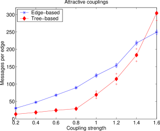
(a)

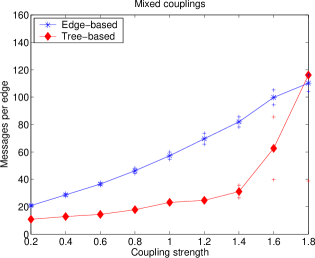
(b)

Figure 6: Comparison of parallel edge-based message-passing (Algorithm  2) and tree-based updates (Algorithm  3  described in Appendix -C) on a nearest-neighbor grid with $n=400$ variables. (a) Attractive couplings. (b) Mixed couplings.

Our comparison is between the parallel edge-based form of reweighted message-passing (Algorithm  2), and the tree-based Algorithm  3  described in Appendix -C. We focus on the amount of computation, as measured by the number of messages passed along each edge, required to either compute the fixed point (up to $\epsilon=1\times 10^{-8}$ accuracy), or—in the case of tree-based updates—to find a configuration ${{\mathbf{x}}}^{*}$ on which all trees agree. In this latter case, Proposition 1 guarantees that the shared configuration ${{\mathbf{x}}}^{*}$ must be globally MAP-optimal for the original problem, so that there is no need to perform any further message-passing.

We performed trials on problems in the Ising form (2), defined on grids with $n=400$ nodes. For the edge-based updates, we used the uniform setting of edge appearance probabilities $\rho_{st}=\frac{n-1}{|E|}$; for the tree-based updates, we used two spanning trees, one with the horizontal rows plus an connecting column and the rotated version of this tree, placing weight $\rho(T^{i})=\frac{1}{2}$ on each tree $i=1,2$. In each trial, the single node potentials were chosen randomly as $\theta_{s}\sim\mathcal{U}[-1,1]$, whereas the edge couplings were chosen in one of the following two ways. In the attractive case, we chose the couplings as $\theta_{st}\sim\mathcal{U}[0,\gamma]$, where $\gamma\geq 0$ is the edge strength. In the mixed case, we chose $\theta_{st}\sim\mathcal{U}[-\frac{\gamma}{2},\frac{\gamma}{2}]$. In both cases, we used damped forms of the updates (linearly combining messages or pseudo-max-marginals in the logarithmic domain) with damping parameter $\lambda=0.50$.

We investigated the algorithmic performance for a range of coupling strengths $\gamma$ for both attractive and mixed cases. For the attractive case, the TRW algorithm is theoretically guaranteed [33] to always find an optimal MAP configuration. For the mixed case, the average fraction of variables in the MAP optimal solution that the reweighted message-passing recovered was above $80\%$ for all the examples that we considered; for mixed problems with weaker observation terms $\theta_{s}$, this fraction can be lower [33, see]. Figure 6 shows results comparing the behavior of the edge-based and tree-based updates. In each panel, plotted on the $y$-axis is the number of messages passed per edge (before achieving the stopping criterion) versus the coupling strength $\gamma$. Note that for more weakly coupled problems, the tree-based updates consistently find the MAP optimum with lower computation than the edge-based updates. As the coupling strength is increased, however, the performance of the tree-based updates slows down and ultimately becomes worse than the edge-based updates. In fact, for strong enough couplings, we observed on occasion that the tree-based updates could fail to converge, but instead oscillate (even with small damping parameters). These empirical observations are consistent with subsequent observations and results by Kolmogorov [31], who developed a modified form of tree-based updates for which certain convergence properties are guaranteed. (In particular, in contrast to the tree-based schedule given in Appendix -C, they are guaranteed to generate a monotonically non-increasing sequence of upper bounds.)

V-D3 Related work

In related work involving the methods described here, we have found several applications in which the tree relaxation and iterative algorithms described here are useful. For instance, we have applied the tree-reweighted max-product algorithm to a distributed data association problem involving multiple targets and sensors [13]. For the class of problem considered, the tree-reweighted max-product algorithm converges, typically quite rapidly, to a provably MAP-optimal data association. In other colloborative work, we have also applied these methods to decoding turbo-like and low density parity check (LDPC) codes [19, 18, 20], and provided finite-length performance guarantees for particular codes and channels. In the context of decoding, the fractional vertices of the polytope $\operatorname{LOCAL}(G)$ have a very concrete interpretation as pseudocodewords [22, 25, 29, 45, e.g.,]. More broadly, it remains to further explore and analyze the range of problems for which the iterative algorithms and LP relaxations described here are suitable.

VI Discussion

In this paper, we demonstrated the utility of convex combinations of tree-structured distributions in upper bounding the value of the maximum a posteriori (MAP) configuration on a Markov random field (MRF) on a graph with cycles. A key property is that this upper bound is tight if and only if the collection of tree-structured distributions shares a common optimum. Moreover, when the upper bound is tight, then a MAP configuration can be obtained for the original MRF on the graph with cycles simply by examining the optima of the tree-structured distributions. This observation motivated two approaches for attempting to obtain tight upper bounds, and hence MAP configurations. First of all, we proved that the Lagrangian dual of the problem is equivalent to a linear programming (LP) relaxation, wherein the marginal polytope associated with the original MRF is replaced with a looser constraint set formed by tree-based consistency conditions. Interestingly, this constraint set is equivalent to the constraint set in the Bethe variational formulation of the sum-product algorithm [47]; in fact, the LP relaxation itself can be obtained by taking a suitable limit of the “convexified” Bethe variational problem analyzed in our previous work [41, 44]. Second, we developed a family of tree-reweighted max product algorithms that reparameterize a collection of tree-structured distributions in terms of a common set of pseudo-max-marginals on the nodes and edges of the graph with cycles. When it is possible to find a configuration that is locally optimal with respect to every single node and edge pseudo-max-marginal, then the upper bound is tight, and the MAP configuration can be obtained. Under this condition, we proved that fixed points of these message-passing algorithms specify dual-optimal solutions to the LP relaxation. A corollary of this analysis is that the ordinary max-product algorithm, when applied to trees, is solving the Lagrangian dual of an exact LP formulation of the MAP estimation problem.

Finally, in cases in which the methods described here do not yield MAP configurations, it is natural to consider strengthening the relaxation by forming clusters of random variables, as in the Kikuchi approximations described by Yedidia et al. [47]. In the context of this paper, this avenue amounts to taking convex combinations of hypertrees, which (roughly speaking) correspond to trees defined on clusters of nodes. Such convex combinations of hypertrees lead, in the dual reformulation, to a hierarchy of progressively tighter LP relaxations, ordered in terms of the size of clusters used to form the hypertrees. On the message-passing side, it is also possible to develop hypertree-reweighted forms of generalizations of the max-product algorithm.

Acknowledgments: We thank Jon Feldman and David Karger for helpful discussions.

-A Conversion from factor graph to pairwise interactions

In this appendix, we briefly describe how any factor graph description of a distribution over a discrete (multinomial) random vector can be equivalently described in terms of a pairwise Markov random field [23], to which the pairwise LP relaxation based on $\operatorname{LOCAL}(G)$ specified by equations (9a),  (9b) and (10) can be applied. To illustrate the general principle, it suffices to show how to convert a factor $f_{123}$ defined on the triplet $\{X_{1},X_{2},X_{3}\}$ of random variables into a pairwise form. Say that each $X_{i}$ takes values in some finite discrete space ${\mathcal{X}}_{i}$.

Given the factor graph description, we associate a new random variable $Z$ with the factor node $f$, which takes values in the Cartesian product space $\mathcal{Z}:={\mathcal{X}}_{1}\times{\mathcal{X}}_{2}\times{\mathcal{X}}_{3}$. In this way, each possible value $z$ of $Z$ can be put in one-to-one correspondence with a triplet $(z_{1},z_{2},z_{3})$, where $z_{i}\in{\mathcal{X}}_{i}$. For each $s\in\{1,2,3\}$, we define a pairwise compatibility function $\psi_{fs}$, corresponding to the interaction between $Z$ and $X_{s}$, by

$$\psi_{fs}(z,x_{s}):=\mathbb{I\,}[z_{s}=x_{s}],$$

where $\mathbb{I\,}[z_{s}=x_{s}]$ is a $\{0,1\}$-valued indicator function for the event $\{z_{s}=x_{s}\}$. We set the singleton compatility functions as

$$\psi_{f}(z)=f(z_{1},z_{2},z_{3}),\quad\mbox{and}\quad\psi_{s}(x_{s})=1.$$

With these definitions, it is straightforward to verify that the augmented distribution given by

$$\psi_{f}(z)\;\prod_{s=1}^{3}\psi_{s}(x_{s})\;\prod_{s=1}^{3}\psi_{fs}(z,x_{s})$$ (61)

marginalizes down to $f(x_{1},x_{2},x_{3})$. Thus, our augmented model with purely pairwise interactions faithfully captures the interaction among the triplet $\{x_{1},x_{2},x_{3}\}$.

Finally, it is straightforward to verify that if we apply the pairwise LP relaxation based on $\operatorname{LOCAL}(G)$ to the augmented model (61), it generates an LP relaxation in terms of the $x_{i}$ variables that involves singleton pseudomarginal distributions $\tau_{s}$, and a pseudomarginal $\tau_{N(f)}$ over the variable neighborhood of each factor $f$. These pseudomarginals are required to be non-negative, normalized to one, and to satisfy the pairwise consistency conditions

$$\sum_{x_{t},\;t\in N(f)\backslash\{s\}}\tau(x_{N(f)}) = \tau_{s}(x_{s})$$ (62)

for all $s\in N(f)$, and for all factor nodes $f$. When the factor graph defines an LDPC code, this procedure generates the LP relaxation studied in Feldman et al. [20]. More generally, this LP relaxation can be applied to factor graph distributions other than those associated with LDPC codes.

-B Proof of Lemma 2

By definition, we have $\Phi_{\infty}({\theta}({T})):=\max_{{{\mathbf{x}}}\in{\mathcal{X}}^{n}}\langle{\theta}({T}),\,{\boldsymbol{\phi}}({{\mathbf{x}}})\rangle$. We re-write this function in the following way:

$$\Phi_{\infty}({\theta}({T})) \overset{(a)}{=} \max_{\tau\in\operatorname{LOCAL}(G)}\langle{\theta}({T}),\,\tau\rangle$$

$$\overset{(b)}{=} \max_{\tau\in\operatorname{LOCAL}(G;T)}\langle{\theta}({T}),\,\tau\rangle$$

where equality (a) follows from Lemma 1, and equality (b) follows because ${\theta}({T})_{\alpha}=0$ for all $\alpha\notin\mathcal{I}(T)$. In this way, we recognize $\Phi_{\infty}({\theta}({T}))$ as the support function of the set $\operatorname{LOCAL}(G;T)$, from which it follows [28] that the conjugate dual is the indicator function of $\operatorname{LOCAL}(G;T)$, as specified in equation (29).

For the sake of self-containment, we provide an explicit proof of this duality relation here. If $\tau$ belongs to $\operatorname{LOCAL}(G;T)$, then $\langle{\theta}({T}),\,\tau\rangle-\Phi_{\infty}({\theta}({T}))\;\leq\;0$ holds for all ${\theta}({T})\in\mathcal{E}(T)$, with equality for ${\theta}({T})=0$. From this relation, we conclude that

$$\sup_{{\theta}({T})\in\mathcal{E}(T)}\langle{\theta}({T}),\,\tau\rangle-\Phi_{\infty}({\theta}({T}))=0$$

whenever $\tau\in\operatorname{LOCAL}(G;T)$.

On the other hand, if $\tau\notin\operatorname{LOCAL}(G;T)$, then by the (strong) separating hyperplane theorem [28], there must exist some vector $\gamma$ and constant $\beta$ such that (i) $\;\langle\gamma,\,\mu\rangle\leq\beta$ for all $\mu\in\operatorname{LOCAL}(G;T)$; and (ii) $\;\langle\gamma,\,\tau\rangle>\beta$. Since conditions (i) and (ii) do not depend on elements $\gamma_{\alpha}$ with $\alpha\notin\mathcal{I}(T)$, we can take $\gamma\equiv{\gamma}({T})\in\mathcal{E}(T)$ without loss of generality. We then have

$$\langle{\gamma}({T}),\,\tau\rangle-\Phi_{\infty}({\gamma}({T}))\;\geq\;\langle{\gamma}({T}),\,\tau\rangle-\beta\>>\;0.$$ (63)

Note that conditions (i) and (ii) are preserved under scaling of both $\gamma(T)$ and $\beta$ by a positive number, so that can send the quantity (63) to positive infinity. We thus conclude that

$$\sup_{\theta(T)\in\mathcal{E}(T)}\big{\{}\langle{\theta}({T}),\,\tau\rangle-\Phi_{\infty}({\theta}({T}))\big{\}}\;=\;+\infty$$

whenever $\tau\notin\operatorname{LOCAL}(G;T)$. This completes the proof of the lemma.

-C Tree-based updates

This appendix provides a detailed description of tree-based updates. In this scheme, each iteration involves multiple rounds of message-passing on each tree $T$ in the support of ${\boldsymbol{\rho}}$. More specifically, the computational engine used within each iteration is the ordinary max-product algorithm, applied as an exact technique to compute max-marginals for each tree-structured distribution.

At any iteration $n$, we let $\theta^{n}(T)$ denote a set of exponential parameters for the tree $T$. To be clear, the notation $\theta^{n}(T)$ used in this appendix differs slightly from its use in the main text. In particular, unlike in the main text, we can have $\theta^{n}_{\alpha}(T)\neq\theta^{n}_{\alpha}(T^{\prime})$ for distinct trees $T=T^{\prime}$ at immediate iterations, although upon convergence this equality will hold. Each step of the algorithm will involve computing, for every tree $T\in\operatorname{supp}({\boldsymbol{\rho}})$, the max-marginals $\nu^{n}(T)$, associated with the tree-structured distribution $p({{\mathbf{x}}};\theta(T))$. (Once again, unlike the main text, we need not have $\nu_{\alpha}^{n}(T)=\nu_{\alpha}^{n}(T^{\prime})$ for distinct trees $T=T^{\prime}$.) Overall, the tree-based updates take the form given in Figure 7.

Algorithm  3: Tree-based updates
1. For each spanning tree $T\in\operatorname{supp}({\boldsymbol{\rho}})$, initialize $\theta^{0}(T)$ via $\displaystyle\theta^{0}_{s}(T)$ $\displaystyle=$ $\displaystyle\bar{\theta}_{s}\;\;\forall\;\;s\in V,$ $\displaystyle\theta^{0}_{st}(T)$ $\displaystyle=$ $\displaystyle\frac{1}{\rho_{st}}\bar{\theta}_{\alpha}\;\;\forall\;\;(s,t)\in E(T),\qquad\qquad\quad\theta^{0}_{st}(T)\;=\;0\;\;\forall\;\;(s,t)\in E\backslash E(T).$ 2. For iterations $n=0,1,2,\ldots$, do the following: (a) For each tree $T\in\operatorname{supp}({\boldsymbol{\rho}})$, apply the ordinary max-product algorithm to compute the max-marginals $\nu^{n}(T)$ corresponding to the tree-structured distribution $p({{\mathbf{x}}};\theta^{n}(T))$. (b) Check if the tree distributions share a common optimizing configuration (i.e., if $\cap_{T}\operatorname{OPT}(\theta^{n}(T))$ is non-empty).
(i) If yes, output any shared configuration and terminate.
(ii) If not, check to see whether or not the following agreement condition holds: $\displaystyle\nu_{s}(T)$ $\displaystyle=$ $\displaystyle\nu_{s}(T^{\prime})\qquad\forall\;s\in V,\qquad\forall T,T^{\prime}\in\operatorname{supp}({\boldsymbol{\rho}}),$ (64a) $\displaystyle\nu_{st}(T)$ $\displaystyle=$ $\displaystyle\nu_{st}(T^{\prime})\qquad\forall\;T,\;T^{\prime}\;\in\;\operatorname{supp}({\boldsymbol{\rho}})\;\operatorname{s.t.}\;(s,t)\in E(T)\cap E(T^{\prime}).$ (64b) If this agreement of all max-marginals holds, then terminate. Otherwise, form a new exponential parameter ${\widetilde{\theta}}$ as follows: $\displaystyle{\widetilde{\theta}}^{n+1}_{s}$ $\displaystyle=$ $\displaystyle\sum_{T}\rho(T)\log\nu^{n}_{s}(T)\;\;\forall\;\;s\in V$ (65a) $\displaystyle{\widetilde{\theta}}^{n+1}_{st}$ $\displaystyle=$ $\displaystyle\sum_{T\ni(s,t)}\rho(T)\log\frac{\nu^{n}_{st}(T)}{\nu^{n}_{s}(T)\nu^{n}_{t}(T)}\;\;\forall\;\;(s,t)\in E$ (65b) Define $\theta^{n+1}(T)$ on each tree $T\in\operatorname{supp}({\boldsymbol{\rho}})$ as in Step 1 with $\bar{\theta}\equiv{\widetilde{\theta}}$, and proceed to Step 2(a).

Figure 7: Tree-based updates for finding a tree-consistent set of pseudo-max-marginals.

Termination: Observe that there are two possible ways in which Algorithm  3  can terminate. On one hand, the algorithm stops if in Step 2(b)(i), a collection of tree-structured distributions is found that all share a common optimizing configuration. Herein lies the possibility of finite termination, since there is no need to wait until the values of the tree max-marginals $\nu^{n}(T)$ all agree for every tree. Otherwise, the algorithm terminates in Step 2(b)(ii) if the max-marginals for each tree all agree with one another, as stipulated by equation (64).

A key property of the updates in Algorithm  3  is that they satisfy the ${\boldsymbol{\rho}}$-reparameterization condition:

Lemma 11

For any iteration $n$, the tree-structured parameters $\{\theta^{n}(T)\}$ of Algorithm  3  satisfy $\sum_{T}\rho(T)\theta^{n}(T)=\bar{\theta}$.

Proof:

The claim for $n=0$ follows from directly the initialization in Step 1. In particular, we clearly have $\sum_{T}\rho(T)\theta^{0}_{s}(T)=\bar{\theta}_{s}$ for any node $s\in V$. For any edge $(s,t)\in E$, we compute:

$$\sum_{T}\rho(T)\theta^{0}_{st}(T)\;=\;\sum_{T}\rho(T)\big{[}\frac{1}{\rho_{st}}\bar{\theta}_{st}]\;=\;\bar{\theta}_{st}.$$

To establish the claim for $n+1$, we proceed by induction. By the claim just proved, it suffices to show that ${\widetilde{\theta}}$, as defined in equation (65), defines the same distribution as $\bar{\theta}$.

We begin by writing $\langle{\widetilde{\theta}},\,{\boldsymbol{\phi}}({{\mathbf{x}}})\rangle$ as

$$\sum_{s\in V}\sum_{x_{s}}{\widetilde{\theta}}_{s}(x_{s})+\sum_{(s,t)\in E}\sum_{x_{s},x_{t}}{\widetilde{\theta}}_{st}(x_{s},x_{t})$$

Using the definition (65), we can re-express it as follows

$$\sum_{T}\rho(T)\Biggr{\{}\sum_{s\in V}\sum_{x_{s}}\log\nu^{n}_{s}(T)(x_{s})\\ +\sum_{(s,t)\in E(T)}\sum_{x_{s},x_{t}}\log\frac{\nu^{n}_{st}(T)(x_{s},x_{t})}{\nu^{n}_{s}(T)(x_{s})\nu^{n}_{t}(T)(x_{t})}\Biggr{\}}$$ (66)

Recall that for each tree $T$, the quantities $\nu^{n}(T)$ are the max-marginals associated with the distribution $p({{\mathbf{x}}};\theta(T))$. Using the fact (36) that the max-marginals specify a reparameterization of $p({{\mathbf{x}}};\theta^{n}(T))$, each term within curly braces is simply equal (up to an additive constant independent of ${{\mathbf{x}}}$) to $\langle\theta^{n}(T),\,{\boldsymbol{\phi}}({{\mathbf{x}}})\rangle$. Therefore, by the induction hypothesis, the RHS of equation (66) is equal to $\langle\bar{\theta},\,{\boldsymbol{\phi}}({{\mathbf{x}}})\rangle$, so that the claim of the lemma follows. ∎

On the basis of Lemma 11, it is straightforward to prove the analog of Theorem 2(a) for Algorithm  3. More specifically, whenever it outputs a configuration, it must be an exact MAP configuration for the original problem $p({{\mathbf{x}}};\bar{\theta})$.

-D Proof of Lemma 9

We first prove an intermediate result:

Lemma 12

Let $\nu^{*}_{s}$ and $\nu^{*}_{st}$ represent pseudo-max-marginals, as defined as in equation (48), with the message $M^{*}:=\exp(\omega^{*})$, where the exponential is taken element-wise. Then the Lagrangian ${\mathcal{L}}_{\bar{\theta},{\boldsymbol{\rho}}}(\tau,\omega^{*})$ can be written as

$$\sum_{T}\rho(T)\mathcal{G}(\tau,\omega^{*};T)+\sum_{s}\kappa_{s}\sum_{x_{s}}\tau_{s}(x_{s})+\sum_{(s,t)}\kappa_{st}\sum_{x_{s},x_{t}}\tau_{st}(x_{s},x_{t})$$

where $\kappa_{s}$ and $\kappa_{st}$ are constants, and $\mathcal{G}(\tau,\omega^{*};T)$ is given by

$$\sum_{s\in V}\sum_{x_{s}}\tau_{s}(x_{s})\log\nu^{*}_{r}(x_{r})\;+\;\\ \sum_{(s,t)\in E(T)}\sum_{(x_{s},x_{t})}\tau_{st}(x_{s},x_{t})\log\frac{\nu^{*}_{st}(x_{s},x_{t})}{\nu^{*}_{s}(x_{s})\nu^{*}_{t}(x_{t})}.$$

Proof:

Straightforward algebraic manipulation allows us to re-express the Lagrangian ${\mathcal{L}}_{\bar{\theta},{\boldsymbol{\rho}}}(\tau,\lambda)$ as

$$\sum_{T}\rho(T)\;\Biggr{\{}\sum_{s\in V}\sum_{x_{s}}\tau_{s}(x_{s})\big{[}\bar{\theta}_{s}(x_{s})+\sum_{t\in\Gamma(s)}\rho_{st}\omega^{*}_{ts}(x_{s})\big{]}\\ +\sum_{(s,t)\in E(T)}\Big{[}\sum_{x_{s},x_{t}}\tau_{st}(x_{s},x_{t})\big{[}\frac{\bar{\theta}_{st}(x_{s},x_{t})}{\rho_{st}}-\omega^{*}_{st}(x_{t})-\omega^{*}_{ts}(x_{s})\big{]}\Big{]}\Biggr{\}}.$$

Using the definition of $\nu^{*}$ in terms of $M^{*}=\exp(\omega^{*})$, we can then write ${\mathcal{L}}_{\bar{\theta},{\boldsymbol{\rho}}}(\tau,\omega^{*})$ in terms of $\mathcal{G}(\tau,\omega^{*};T)$ as

$$\sum_{T}\rho(T)\mathcal{G}(\tau,\omega^{*};T)+\sum_{s}\kappa_{s}\sum_{x_{s}}\tau_{s}(x_{s})+\\ \sum_{(s,t)}\kappa_{st}\sum_{x_{s},x_{t}}\tau_{st}(x_{s},x_{t}),$$

where the constants $\kappa_{s}$ and $\kappa_{st}$ arise from the normalization of $\nu^{*}_{s}$ and $\nu^{*}_{st}$. ∎

Recall that we root all trees $T$ a fixed vertex $r\in V$, so that each vertex $s\neq r$ has a unique parent denoted $\pi^{T}(s)$. Using the parent-to-child representation of the tree $T$, we can re-express $\mathcal{G}(\tau,\omega^{*};T)$ as

$$\Big{\{}\sum_{x_{r}}\tau_{r}(x_{r})\log\nu^{*}_{r}(x_{r})+\\ \sum_{(s,\pi^{T}(s))}\sum_{(x_{s},x_{\pi^{T}(s)})}\tau_{st}(x_{s},x_{t})\log\frac{\nu^{*}_{s\pi^{T}(s)}(x_{s},x_{\pi^{T}(s)})}{\nu^{*}_{\pi^{T}(s)}(x_{\pi^{T}(s)})}\Big{\}}+\\ \sum_{s\neq r}\sum_{x_{s}}\log\nu^{*}_{s}(x_{s})\big{[}\tau_{s}(x_{s})-\sum_{x_{t}}\tau_{st}(x_{s},x_{t})\big{]}$$

Recalling the definition of $\mathcal{F}_{\bar{\theta};{\boldsymbol{\rho}}}(\tau,\nu;T)$ from equation (55), we can write $\sum_{T}\rho(T)\mathcal{G}(\tau;\omega^{*};T)$ as

$$\sum_{T}\rho(T)\mathcal{F}_{\bar{\theta};{\boldsymbol{\rho}}}(\tau,\nu^{*};T)+\\ \sum_{T}\rho(T)\sum_{s\neq r}\sum_{x_{s}}\log\nu^{*}_{s}(x_{s})\big{[}\tau_{s}(x_{s})-\sum_{x_{t}}\tau_{st}(x_{s},x_{t})\big{]},$$

or equivalently as

$$\sum_{T}\rho(T)\mathcal{F}_{\bar{\theta};{\boldsymbol{\rho}}}(\tau,\nu^{*};T)+\\ \sum_{(s,t)\in E}\sum_{x_{s}}\big{(}\sum_{\{T\,|t=\pi^{T}(s)\}}\rho(T)\big{)}\log\nu^{*}_{s}(x_{s})C_{ts}(x_{s}),$$

where $C_{ts}(x_{s})=\tau_{s}(x_{s})-\sum_{x_{t}}\tau_{st}(x_{s},x_{t})$ is the constraint. Note that for each fixed $(s,t)$ and $x_{s}$ the term $\sum_{\{T\,|t=\pi^{T}(s)\}}\rho(T)\log\nu^{*}_{s}(x_{s})$ can be interpreted as a contribution to the Lagrange multiplier associated with the constraint $C_{ts}(x_{s})$.

Finally, since the Lagrangian is linear in the Lagrange multipliers, we can use Lemma 12 to express the Lagrangian ${\mathcal{L}}_{\bar{\theta},{\boldsymbol{\rho}}}(\tau,\lambda^{*};T)$ as

$$\sum_{T}\rho(T)\mathcal{F}_{\bar{\theta};{\boldsymbol{\rho}}}(\tau,\nu^{*};T)+\sum_{s}\kappa_{s}\sum_{x_{s}}\tau_{s}(x_{s})+\\ \sum_{(s,t)}\kappa_{st}\sum_{x_{s},x_{t}}\tau_{st}(x_{s},x_{t}),$$

where $\lambda^{*}$ is the vector of Lagrange multipliers with components

$$\lambda^{*}_{ts}(x_{s}):=\omega^{*}_{ts}(x_{s})-\sum_{\{T\,\big{|}\,\pi^{T}(s)=t\}}\rho(T)\log\nu^{*}_{s}(x_{s}).$$

-E Proof of Lemma 10

Since by assumption the pseudo-max-marginals $\nu^{*}$ defined by $M^{*}=\exp(\lambda^{*})$ (with the exponential defined element-wise) satisfy the optimum specification criterion, we can find a configuration ${{\mathbf{x}}}^{*}$ that satisfies the local optimality conditions (38) for every node and edge on the full graph $G$.

Since the pseudo-max-marginals $\nu^{*}$ are defined by a fixed point $M^{*}=\exp(\lambda^{*})$ (with the exponential defined element-wise) of the update equation (50), the pseudo-max-marginals must be pairwise-consistent. More explicitly, for any edge $(s,t)$ and $x_{s}\in{\mathcal{X}}_{s}$, the pairwise consistency condition $\max_{x_{t}}\nu^{*}_{st}(x_{s},x_{t})=\kappa_{st}\;\nu^{*}(x_{s})$ holds, where $\kappa_{st}$ is a positive constant independent of $x_{s}$. Using this fact, we can write

$$\max_{x_{s},x_{t}}\log\frac{\nu^{*}_{st}(x_{s},x_{t})}{\nu^{*}_{s}(x_{s})} = \max_{x_{s}}\log\frac{\max_{x_{t}}\nu^{*}_{st}(x_{s},x_{t})}{\nu^{*}_{s}(x_{s})}$$ (67)

$$= \log\kappa_{st}.$$

Moreover, since by assumption the pseudo-max-marginals $\nu^{*}$ satisfy the optimum specification criterion, we can find a configuration ${{\mathbf{x}}}^{*}$ that satisfies the local optimality conditions (38) for every node and edge on the full graph $G$. For this configuration, we have the equality

$$\max_{x_{s}}\log\nu^{*}_{s}(x_{s})=\log\nu^{*}_{s}(x^{*}_{s})\qquad\mbox{for all $s\in V$},$$ (68)

and

$$\log\frac{\nu_{st}^{*}(x^{*}_{s},x^{*}_{t})}{\nu_{s}^{*}(x^{*}_{s})} = \log\frac{\max_{x_{t}}\nu_{st}^{*}(x^{*}_{s},x_{t})}{\nu_{s}^{*}(x^{*}_{s})}$$ (69)

$$= \log\kappa_{st}$$

$$= \max_{x_{s},x_{t}}\log\frac{\nu^{*}_{st}(x_{s},x_{t})}{\nu^{*}_{s}(x_{s})}$$

for all $(s,t)\in E$, where the final equality follows from equation (67).

Recall the definition of $\tau^{*}$ from equation (57a). Using equations (68) and (69), we have

$$\sum_{x_{s}}\tau_{s}(x_{s})\log\nu^{*}_{s}(x_{s}) \leq \sum_{x_{s}}\tau^{*}_{s}(x_{s})\log\nu^{*}_{s}(x_{s})$$ (70)

for all $s\in V$, and

$$\sum_{x_{s},x_{t}}\tau_{s}(x_{s},x_{t})\log\frac{\nu^{*}_{st}(x_{s},x_{t})}{\nu^{*}_{s}(x_{s})}\\ \leq\sum_{x_{s},x_{t}}\tau^{*}_{s}(x_{s},x_{t})\log\frac{\nu^{*}_{st}(x_{s},x_{t})}{\nu^{*}_{s}(x_{s})}$$ (71)

for all $(s,t)\in E$. Both equations (70) and (71) hold for all $\tau\in\mathcal{S}$ (i.e., for all non-negative $\tau$ such that $\sum_{x_{s}}\tau_{s}(x_{s})=1$ and $\sum_{x_{s},x_{t}}\tau_{st}(x_{s},x_{t})=1$). Finally, inequalities (70) and (71) imply that $\max_{\tau\in\mathcal{S}}\mathcal{F}(\tau,\nu^{*};T)=\mathcal{F}(\tau^{*},\nu^{*};T)$ as claimed.

References

- [1] S. M. Aji, G. Horn, R. J. McEliece, and M. Xu. Iterative min-sum decoding of tail-biting codes. In Proc. IEEE Information Theory Workshop, Killarney Ireland, pages 68–69, June 1998.
- [2] S.M. Aji and R.J. McEliece. The generalized distributive law. IEEE Trans. Info. Theory, 46:325–343, March 2000.
- [3] S. Amari. Information geometry on a hierarchy of probability distributions. IEEE Trans. on Information Theory, 47(5):1701–1711, 2001.
- [4] O. E. Barndorff-Nielson. Information and exponential families. Wiley, Chichester, 1978.
- [5] R. J. Baxter. Exactly solved models in statistical mechanics. Academic Press, New York, 1982.
- [6] D.P. Bertsekas. Nonlinear programming. Athena Scientific, Belmont, MA, 1995.
- [7] D. Bertsimas and J. Tsitsikilis. Introduction to linear optimization. Athena Scientific, Belmont, MA, 1997.
- [8] J. Besag. On the statistical analysis of dirty pictures. Journal of the Royal Statistical Society, Series B, 48(3):259–279, 1986.
- [9] N. Biggs. Algebraic graph theory. Cambridge University Press, Cambridge, 1993.
- [10] B. Bollobás. Modern graph theory. Springer-Verlag, New York, 1998.
- [11] E. Boros, Y. Crama, and P. L. Hammer. Upper bounds for quadratic 0-1 maximization. Operations Research Letters, 9:73–79, 1990.
- [12] P. Brémaud. Markov chains, Gibbs fields, Monte Carlo simulation, and queues. Springer, 1991.
- [13] L. Chen, M. J. Wainwright, M. Cetin, and A. Willsky. Multitarget-multisensor data association using the tree-reweighted max-product algorithm. In SPIE Aerosense Conference, April 2003.
- [14] R. G. Cowell, A. P. Dawid, S. L. Lauritzen, and D. J. Spiegelhalter. Probabilistic Networks and Expert Systems. Statistics for Engineering and Information Science. Springer-Verlag, 1999.
- [15] A. P. Dawid. Applications of a general propagation algorithm for probabilistic expert systems. Statistics and Computing, 2:25–36, 1992.
- [16] M. Deza and M. Laurent. Geometry of Cuts and Metric Embeddings. Springer-Verlag, New York, 1997.
- [17] J. Edmonds. Matroids and the greedy algorithm. Mathematical Programming, 1:127–136, 1971.
- [18] J. Feldman, D. R. Karger, and M. J. Wainwright. Using linear programming to decode LDPC codes. In Conference on Information Science and Systems, March 2003.
- [19] J. Feldman, M. J. Wainwright, and D. R. Karger. Linear programming-based decoding of turbo-like codes and its relation to iterative approaches. In Proc. Allerton Conf. Comm., Control and Computing, October 2002.
- [20] J. Feldman, M. J. Wainwright, and D. R. Karger. Using linear programming to decode binary linear codes. IEEE Transactions on Information Theory, 51:954–972, March 2005.
- [21] G. D. Forney, Jr., F. R. Kschischang, B. Marcus, and S. Tuncel. Iterative decoding of tail-biting trellises and connections with symbolic dynamics. In Codes, systems and graphical models, pages 239–264. Springer, 2001.
- [22] G.D. Forney, Jr., R. Koetter, F. R. Kschischang, and A. Reznick. On the effective weights of pseudocodewords for codes defined on graphs with cycles. In Codes, systems and graphical models, pages 101–112. Springer, 2001.
- [23] W. T. Freeman and Y. Weiss. On the optimality of solutions of the max-product belief propagation algorithm in arbitrary graphs. IEEE Trans. Info. Theory, 47:736–744, 2001.
- [24] B. J. Frey and R. Koetter. Exact inference using the attenuated max-product algorithm. In Advanced mean field methods: Theory and Practice. MIT Press, 2000.
- [25] B. J. Frey, R. Koetter, and A. Vardy. Signal-space characterization of iterative decoding. IEEE Trans. Info. Theory, 47:766–781, 2001.
- [26] D. M. Greig, B. T. Porteous, and A. H. Seheuly. Exact maximum a posteriori estimation for binary images. Journal of the Royal Statistical Society B, 51:271–279, 1989.
- [27] P.L. Hammer, P. Hansen, and B. Simeone. Roof duality, complementation, and persistency in quadratic 0-1 optimization. Mathematical Programming, 28:121–155, 1984.
- [28] J. Hiriart-Urruty and C. Lemaréchal. Convex analysis and minimization algorithms, volume 1. Springer-Verlag, New York, 1993.
- [29] G. Horn. Iterative decoding and pseudocodewords. PhD thesis, California Institute of Technology, 1999.
- [30] R. Koetter and P. O. Vontobel. Graph-covers and iterative decoding of finite length codes. In Proc. 3rd International Symp. on Turbo Codes, September 2003.
- [31] V. Kolmogorov. Convergent tree-reweighted message-passing for energy minimization. In International Workshop on Artificial Intelligence and Statistics, January 2005.
- [32] V. Kolmogorov. Convergent tree-reweighted message-passing for energy minimization. Technical report, Microsoft Research, January 2005. Submitted to IEEE PAMI.
- [33] V. Kolmogorov and M. J. Wainwright. On optimality properties of tree-reweighted message-passing. In Uncertainty in Artificial Intelligence, July 2005.
- [34] S. L. Lauritzen. Graphical Models. Oxford University Press, Oxford, 1996.
- [35] R.J. McEliece, D.J.C. McKay, and J.F. Cheng. Turbo decoding as an instance of Pearl’s belief propagation algorithm. IEEE Jour. Sel. Comm., 16(2):140–152, February 1998.
- [36] T. Minka. Power ep. Technical report, Carnegie Mellon University, Department of Statistics, 2004.
- [37] G. Rockafellar. Convex Analysis. Princeton University Press, Princeton, 1970.
- [38] A. Schrijver. Combinatorial Optimization: Polyhedra and Efficiency. Springer-Verlag, New York, NY, 2003.
- [39] S. Verdú. Multiuser detection. Cambridge University Press, Cambridge, 1998.
- [40] A. Viterbi. Error bounds for convolutional codes and an asymptotically optimal decoding algorithm. IEEE Trans. Info. Theory, IT-13:260–269, April 1967.
- [41] M. J. Wainwright, T. S. Jaakkola, and A. S. Willsky. A new class of upper bounds on the log partition function. In Uncertainty in Artificial Intelligence, volume 18, pages 536–543, August 2002.
- [42] M. J. Wainwright, T. S. Jaakkola, and A. S. Willsky. Tree-based reparameterization framework for analysis of sum-product and related algorithms. IEEE Trans. Info. Theory, 49(5):1120–1146, May 2003.
- [43] M. J. Wainwright, T. S. Jaakkola, and A. S. Willsky. Tree consistency and bounds on the max-product algorithm and its generalizations. Statistics and Computing, 14:143–166, April 2004.
- [44] M. J. Wainwright, T. S. Jaakkola, and A. S. Willsky. A new class of upper bounds on the log partition function. IEEE Trans. Information Theory, page To appear, July 2005.
- [45] N. Wiberg. Codes and decoding on general graphs. PhD thesis, University of Linkoping, Sweden, 1996.
- [46] W. Wiegerinck and T. Heskes. Fractional belief propagation. In NIPS, volume 12, pages 438–445, 2002.
- [47] J. S. Yedidia, W. T. Freeman, and Y. Weiss. Understanding belief propagation and its generalizations. Technical Report TR2001-22, Mitsubishi Electric Research Labs, January 2002.