Lossy source encoding via message-passing and decimation over generalized codewords of LDGM codes

Abstract

We describe message-passing and decimation approaches for lossy source coding using low-density generator matrix (LDGM) codes. In particular, this paper addresses the problem of encoding a Bernoulli($\frac{1}{2}$) source: for randomly generated LDGM codes with suitably irregular degree distributions, our methods yield performance very close to the rate distortion limit over a range of rates. Our approach is inspired by the survey propagation (SP) algorithm, originally developed by Mézard et al. [1] for solving random satisfiability problems. Previous work by Maneva et al. [2] shows how SP can be understood as belief propagation (BP) for an alternative representation of satisfiability problems. In analogy to this connection, our approach is to define a family of Markov random fields over generalized codewords, from which local message-passing rules can be derived in the standard way. The overall source encoding method is based on message-passing, setting a subset of bits to their preferred values (decimation), and reducing the code.

To appear in International Symposium on Information Theory; Adelaide, Australia

I Introduction

Graphical codes such as turbo and low-density parity check (LDPC) codes, when decoded with the belief propagation or sum-product algorithm, perform close to capacity [3, e.g.,]. Similarly, LDPC codes have been successfully used for various types of lossless compression schemes [4, e.g.,]. One standard approach to lossy source coding is based on trellis codes and the Viterbi algorithm. The goal of this work is to explore the use of codes based on graphs with cycles, whose potential has not yet been fully realized for lossy compression. A major challenge in applying such graphical codes to lossy compression is the lack of practical (i.e., computationally efficient) algorithms for encoding and decoding. Accordingly, our focus is the development of practical algorithms for performing lossy source compression. For concreteness, we focus on the problem of quantizing a Bernoulli source with $p=\frac{1}{2}$. Developing and analyzing effective algorithms for this problem is a natural first step towards solving more general lossy compression problems (e.g., involving continuous sources or memory).

Our approach to lossy source coding is based on the dual codes of LDPC codes, known as low-density generator matrix (LDGM) codes. This choice was partly motivated by an earlier paper of Martinian and Yedidia [5], who considered a source coding “dual” of the BEC channel coding problem. They proved that optimal rate-distortion performance for this problem can be achieved using the LDGM duals of capacity-achieving LDPC codes, and a modified message-passing algorithm. Our work was also inspired by the original survey propagation algorithm [1], and subsequent analysis by Maneva et al. [2] making a precise connection to belief propagation over an extended Markov random field. In recent work, Murayama [6] developed a modified form of belief propagation based on the TAP approximation, and provided results in application to source encoding for LDGM codes with fixed check degree two. In work performed in parallel to the work described here, other research groups have applied forms of survey propagation for source encoding based on codes composed of local non-linear “check” functions [7] and $k$-SAT problems with doping [8].

II Background and set-up

Given a $\operatorname{Ber}(\frac{1}{2})$ source, any particular i.i.d. realization $y\in\{0,1\}^{n}$ is referred to as a source sequence. The goal is to compress source sequences $y$ by mapping them to shorter binary vectors $x\in\{0,1\}^{m}$ with $m<n$, where the quantity $R:=\frac{m}{n}$ is the compression ratio. The source decoder then maps the compressed sequence $x$ to a reconstructed source sequence $\widehat{y}$. For a given pair $(y,\widehat{y})$, the reconstruction fidelity is measured by the Hamming distortion $d_{H}(y,\widehat{y}):=\frac{1}{n}\sum_{i=1}^{n}|y_{i}-\widehat{y}_{i}|$. The overall quality of our encoder-decoder pair is measured by the average Hamming distortion $D:={\mathbb{E}}[d_{H}(Y,\widehat{Y})]$. For the $\operatorname{Ber}(\frac{1}{2})$ source, the rate distortion function is well-known to take the form $R(D)=1-H(D)$ for $D\in[0,0.5]$, and $0$ otherwise.

Our approach to lossy source coding is based on low-density generator matrix codes, hereafter referred to as LDGM codes, which arise naturally as the duals of LDPC codes. For a given rate $R=\frac{m}{n}<1$, let $A$ be an $n\times m$ matrix with $\{0,1\}$ entries, where we assume $\operatorname{rank}A=m$ without loss of generality. The low-density condition requires that the number of $1$s in each row and column is bounded. The matrix $A$ is the generator matrix of the LDGM, thereby defining the code $\mathbb{C}(A):=\{z\in\{0,1\}^{n}\,|\,z=Ax\mbox{ for some $x\in\{0,1\}^{m}$}\}$, where arithmetic is performed over $\operatorname{GF}(2)$. It will also be useful to consider the code over $(x,z)$ given by $\bar{\mathbb{C}}(A):=\{(x,z)\in\{0,1\}^{n+m}\>|\;z=Ax\}$. We refer to elements of $x$ as information bits, and elements of $z$ as source bits. In the LDGM approach to source coding, the encoding phase of the source coding problem amounts to mapping a given source sequence $y\in\{0,1\}^{n}$ to an information vector $x(y)\in\{0,1\}^{m}$. Decoding is straightforward: we simply form $\widehat{y}(x)=Ax$. The challenge lies in the encoding phase: in particular, we must determine the information bit vector $x$ such that the Hamming distortion $\frac{1}{n}\|y-Ax\|_{1}$ is minimized. This combinatorial optimization problem is equivalent to an MAX-XORSAT problem, and hence known to be NP-hard in general.

It is convenient to represent a given LDGM code, specified by generator matrix $A$, as a factor graph $G=(V,C,E)$, where $V=\{1,\ldots,m\}$ denotes the set of information bits and $C:=\{1,\ldots,n\}$ denotes the set of checks (or equivalently, source bits), and $E$ denotes the set of edges between checks and information bits. As illustrated in Figure 1, the $n$ source bits are lined up at the top of the graph, and each is connected to a unique check neighbor. Each check, in turn, is connected to (some subset of) the $m$ information bits at the bottom of the graph. Note that there is a one-to-one correspondence between source bits and checks. We use letters $a,b,c$ to refer to elements of $C$, corresponding either to a source bit or the associated check. Conversely, we use letters $i,j,k$ to refer to information bits in the set $V$. For each information bit $i\in V$, let $C(i)\subseteq C$ denote its check neighbors: $C(i):=\{a\in C\>|\;(a,i)\in E\}$. Similarly, for each check $a\in C$, we define the set $V(a):=\{i\in V\>|\;(a,i)\in E\}$. We use the notation $\bar{V}(a):=V(a)\cup\{a\}$ to denote the set of all bits—both information and source—that are adjacent to check $a$.

III Markov random fields and decimation with generalized codewords

A natural first idea to solving the source encoding problem would be to follow the channel coding approach: run the sum-product algorithm on the ordinary factor graph, and then threshold the resulting log-likelihood ratios (LLRs) at each bit to determine a source encoding $x(\widehat{y})$. Unfortunately, this approach fails: either the algorithm fails to converge or the LLRs fail to yield reliable information, resulting in a poor source encoding. Inspired by survey propagation for satisfiability problems [1], we consider an approach with two components: (a) extending the factor distribution so as to include not just ordinary codewords but also a set of partially assigned codewords, and (b) performing a sequence of message-passing and decimation steps, each of which entails setting fraction of bits to their preferred values.

More specifically, we consider Markov random fields over a larger space of so-called generalized codewords, which are members of the space $\{0,1,\ast\}^{n+m}$ where $\ast$ is a new symbol. As we will see, the interpretation of $x_{i}=\ast$ is that the associated bit $i$ is free. Conversely, any bit for which $x_{i}\in\{0,1\}$ is forced. One possible view of a generalized codeword, as with the survey propagation and $k$-SAT problems, is as an index for a cluster of ordinary codewords. We define a family of Markov random fields, parameterized by a weight for $\ast$-variables, and a weight that measures fidelity to the source sequence. As a particular case, our family of MRFs includes a weighted distribution over the set of ordinary codewords. Although the specific extension considered here is natural to us (and yields good source coding results), it could be worthwhile to consider alternative ways in which to extend the original distribution to generalized codewords.

III-A Generalized codewords

Definition 1 (Check states)

In any generalized codeword, each check is in one of two possible exclusive states:

1. we say that check $a\in C$ is forcing whenever none of its bit neighbors are free, and the local $\{0,1\}$-codeword $(z_{a};x_{V(a)})\in\{0,1\}^{1+|V(a)|}$ satisfies parity check $a$.

2. on the other hand, check $a$ is free whenever $z_{a}=\ast$, and moreover $x_{i}=\ast$ for at least one $i\in V(a)$.

Note that the source bit $z_{a}$ is free (or forced) if and only if the associated check $a$ is free (or forcing). With this set-up, our space of generalized codewords is defined as follows:

Definition 2 (Generalized codeword)

A vector $(z,x)\in\{0,1,\ast\}^{n+m}$ is a valid generalized codeword when the following conditions hold:

1. all checks $a$ are either forcing or free.

2. if some information bit $x_{i}$ is forced (i.e., $x_{i}\in\{0,1\}$), then at at least two check neighbors $a\in C(i)$ must be forcing it.

For a generator matrix in which every information bit has degree two or greater, it can be seen that any ordinary codeword $(z,x)\in\bar{\mathbb{C}}(A)$ is also a generalized codeword. In addition, there are generalized codewords that include $\ast$’s in some positions, and hence do not correspond to ordinary codewords. One such (non-trivial) generalized codeword is illustrated in Figure 1. A natural way in which to generate generalized codewords is via an iterative “peeling” or “leaf-stripping” procedure. Related procedures have been analyzed in the context of satisfiability problems [2], XORSAT problems [9], and for performing binary erasure quantization [5].

Peeling procedure: Given some initial source sequence $z\in\{0,1,\ast\}^{n}$, initialize all information bits $x_{i}$ to be forced.

1. While there exists a forced information bit $x_{i}$ with exactly one forcing check neighbor $a$, set $x_{i}=z_{a}=\ast$.

2. When all remaining forced information bits have at least two forcing checks, go to Step 3.

3. For any free check $z_{a}=\ast$ with no free information bit neighbors, set $z_{a}=\oplus_{i\in V(a)}x_{i}$.

When initialized with at least one free check, Step 1 of this peeling procedure can terminate in one of two possible ways: either the initial configuration is stripped down to the all-$\ast$ configuration, or Step 1 terminates at a configuration such that every forced information bit has two or more forcing check neighbors, thus ensuring that condition (ii) of Definition 2 is satisfied. As noted previously [5], these cores can be viewed as “duals” to stopping sets in the dual LDPC. Finally, Step 3 ensures that every free check has at least one free information bit, thereby satisfying condition (i) of Definition 2.

\psfrag{#i#}{$i$}\psfrag{#j#}{$j$}\psfrag{#k#}{$k$}\psfrag{#l#}{$l$}\psfrag{#a#}{$a$}\psfrag{#b#}{$b$}\psfrag{#c#}{$c$}\psfrag{#d#}{$d$}\psfrag{#e#}{$e$}\psfrag{#f#}{$f$}\psfrag{#g#}{$g$}\psfrag{#*#}{$\ast$}\psfrag{#0#}{$0$}\psfrag{#1#}{$1$}\includegraphics[keepaspectratio,width=138.76157pt]{new_ldgm_extmrf.eps}

Figure 1: Illustration of a generalized codeword for a small LDGM. Information bits $i$ and $j$ are both forced; for each, the two forcing checks are $a$ and $b$. The remaining checks and bits are all free.

III-B Weighted version

Given a particular source sequence $y\in\{0,1\}^{n}$, we form a probability distribution over the set of generalized codewords as follows. For any generalized codeword $(z,x)\in\{0,1,\ast\}^{n+m}$, we define the sets $n_{\ast}^{\operatorname{sou}}(z):=\big{|}\{i\in\{1,\ldots,n\}\,|\,z_{i}=\ast\}\big{|}$ and $n_{\ast}^{\operatorname{info}}(x):=\big{|}\{i\in\{1,\ldots,m\}\,|\,x_{i}=\ast\}\big{|}$, corresponding to the number of $\ast$-variables in the source and information bits respectively. We associate non-negative weights $w_{\operatorname{sou}}$ and $w_{\operatorname{info}}$ with the $\ast$-variables in the source and information bits respectively. Finally, we introduce a non-negative parameter $\gamma$, which will be used to penalize disagreements between the source bits $z$ and the given (fixed) source sequence $y$. Of interest to us in the sequel is the weighted probability distribution

$$p(z,x;w_{\operatorname{sou}},w_{\operatorname{info}},\lambda)\propto w_{\operatorname{sou}}^{n_{\ast}^{\operatorname{sou}}(z)}\times w_{\operatorname{info}}^{n_{\ast}^{\operatorname{info}}(x)}\times\exp^{-2\gamma d_{H}(y,z)}.$$ (1)

Note that for $w_{\operatorname{sou}}=w_{\operatorname{info}}=0$, this distribution reduces to the standard weighted distribution over ordinary codewords.

III-C Representation as Markov random field

We now seek to represent the set of generalized codewords as a Markov random field (MRF). A first important observation is that state augmentation is necessary to achieve such a Markov representation with respect to the original factor graph.

Lemma 1

For positive $w_{\operatorname{sou}},w_{\operatorname{info}}$, the set of generalized codewords cannot be represented as a Markov random field based on the original factor graph $G$ where the state space at each bit is simply $\{0,1,\ast\}$.

Proof:

It suffices to demonstrate that it is impossible to construct an indicator function for membership in the set of generalized codewords as a product of local compatibility functions on $\{0,1,\ast\}$, one for each check. The key is that the set of all local generalized codewords cannot be defined only in terms of the variables $x_{\bar{V}(a)}$; rather, the validity depends also on all bit neighbors of checks that are incident to bits in $\bar{V}(a)$. or more formally on bits with indices in the set

$$\cup_{i\in\bar{V}(a)}\big{\{}j\in V\;\big{|}\;j\in V(b)\mbox{ for some }b\in C(i)\big{\}}.$$ (2)

As a particular illustration, consider the trivial LDGM code consisting of a single source bit (and check) connected to three information bits. From Definition 1 and Definition 2, it can be seen that the only generalized codeword is the all-$\ast$ configuration. Thus, any check function used to define membership in the set of generalized codewords would have to assign zero mass to any other $\{0,1,\ast\}$ configuration. Now suppose that this simple LDGM is embedded within a larger LDGM code. For instance, consider the check labeled $e$ (with source bit $z_{e}$) and corresponding information bits $\{j,k,l\}$ in Figure 1. With respect to the generalized codeword in this figure, we see that the local configuration $(x_{j},x_{k},x_{l}z_{e})=(1,\ast,\ast,\ast)$ is locally valid, which contradicts our conclusion from considering the trivial LDGM code in isolation. Hence, the constraints enforced by a given check change depending on the larger context in which it is embedded. ∎

Consequently, obtaining a factorization of the distribution requires keeping track of variables in the extended set (2). Accordingly, as in the reformulation of survey propagation for SAT problems by Maneva et al. [2], we introduce a new variable $P_{i}$, so that there is a vector $(x_{i},P_{i})$ associated with each bit. To define $P_{i}$, first let $\mathcal{P}(i)=\mathcal{P}(C(i))$ denote the power set of all of the clause neighbors $C(i)$ of bit $i$. (I.e., $\mathcal{P}(i)$ is a set with $2^{|C(i)|}$ elements). The variable $P_{i}$ takes on subsets of $C(i)$, and we decompose it as $P_{i}=P^{0}_{i}\cup P^{1}_{i}$, where at any time at most one of $P^{1}_{i}$ and $P^{0}_{i}$ are non-empty. The variable $P_{i}$ has the following decomposition and interpretation: (a) if $P^{0}_{i}=P^{1}_{i}=\emptyset$, then no checks are forcing bit $x_{i}$; (b) if $P_{i}=P^{1}_{i}\neq\emptyset$, then certain checks are forcing $x_{i}$ to be one (so that necessarily $x_{i}=1$); and (c) similarly, if $P_{i}=P^{0}_{i}\neq\emptyset$, then certain checks are forcing $x_{i}$ to be zero (so that necessarily $x_{i}=0$). By construction, this definition excludes the case that both $P^{0}_{i}$ and $P^{1}_{i}$ non-empty at the same time, so that the state space of $P_{i}$ has cardinality $2^{|C(i)|}+2^{|C(i)|}-1\;=\;2^{|C(i)|+1}-1$.

Bits to checks $\displaystyle M^{0f}_{i\rightarrow a}$ $\displaystyle\leftarrow$ $\displaystyle\lambda^{0}_{i}\Big{\{}\prod_{b\in C(i)\backslash\{a\}}\big{[}M^{0f}_{b\rightarrow i}+M^{0w}_{b\rightarrow i}\big{]}-\prod_{b\in C(i)\backslash\{a\}}M^{0w}_{b\rightarrow i}\Big{\}}$ $\displaystyle M^{1f}_{i\rightarrow a}$ $\displaystyle\leftarrow$ $\displaystyle\lambda^{1}_{i}\Big{\{}\prod_{b\in C(i)\backslash\{a\}}\big{[}M^{1f}_{b\rightarrow i}+M^{1w}_{b\rightarrow i}\big{]}-\prod_{b\in C(i)\backslash\{a\}}M^{1w}_{b\rightarrow i}\Big{\}}$ $\displaystyle M^{0w}_{i\rightarrow a}$ $\displaystyle\leftarrow$ $\displaystyle\lambda^{0}_{i}\Big{\{}\prod_{b\in C(i)\backslash\{a\}}\big{[}M^{0f}_{b\rightarrow i}+M^{0w}_{b\rightarrow i}\big{]}-\prod_{b\in C(i)\backslash\{a\}}M^{0w}_{b\rightarrow i}-\sum_{c\in C(i)\backslash\{a\}}M^{0f}_{c\rightarrow i}\prod_{b\in C(i)\backslash\{a,c\}}M^{0w}_{b\rightarrow i}\Big{\}}.$ $\displaystyle M^{1w}_{i\rightarrow a}$ $\displaystyle\leftarrow$ $\displaystyle\lambda^{1}_{i}\Big{\{}\prod_{b\in C(i)\backslash\{a\}}\big{[}M^{1f}_{b\rightarrow i}+M^{1w}_{b\rightarrow i}\big{]}-\prod_{b\in C(i)\backslash\{a\}}M^{1w}_{b\rightarrow i}-\sum_{c\in C(i)\backslash\{a\}}M^{1f}_{c\rightarrow i}\prod_{b\in C(i)\backslash\{a,c\}}M^{1w}_{b\rightarrow i}\Big{\}}.$ $\displaystyle M^{*}_{i\rightarrow a}$ $\displaystyle\leftarrow$ $\displaystyle w_{\operatorname{info}}\;\prod_{b\in C(i)\backslash\{a\}}M^{*}_{b\rightarrow i}$ Checks to bits $\displaystyle M^{0f}_{a\rightarrow i}$ $\displaystyle\leftarrow$ $\displaystyle\frac{1}{2}\Big{[}\prod_{j\in\bar{V}(a)\backslash\{i\}}\big{(}M^{0f}_{j\rightarrow a}+M^{1f}_{j\rightarrow a}\big{)}+\prod_{j\in\bar{V}(a)\backslash\{i\}}\big{(}M^{0f}_{j\rightarrow a}-M^{1f}_{j\rightarrow a}\big{)}\Big{]}$ $\displaystyle M^{1f}_{a\rightarrow i}$ $\displaystyle\leftarrow$ $\displaystyle\frac{1}{2}\Big{[}\prod_{j\in\bar{V}(a)\backslash\{i\}}\big{(}M^{0f}_{j\rightarrow a}+M^{1f}_{j\rightarrow a}\big{)}-\prod_{j\in\bar{V}(a)\backslash\{i\}}\big{(}M^{0f}_{j\rightarrow a}-M^{1f}_{j\rightarrow a}\big{)}\Big{]}$ $\displaystyle M^{0w}_{a\rightarrow i}$ $\displaystyle\leftarrow$ $\displaystyle\prod_{j\in\bar{V}(a)\backslash\{i\}}\big{[}M^{*}_{j\rightarrow a}+M^{1w}_{j\rightarrow a}+M^{0w}_{j\rightarrow a}\big{]}-\prod_{j\in\bar{V}(a)\backslash\{i\}}\big{[}M^{1w}_{j\rightarrow a}+M^{0w}_{j\rightarrow a}\big{]}-\sum_{k\in\bar{V}(a)\backslash\{i\}}M^{*}_{k\rightarrow a}\prod_{j\in\bar{V}(a)\backslash\{i,k\}}\big{[}M^{1w}_{j\rightarrow a}+M^{0w}_{j\rightarrow a}\big{]}$ $\displaystyle M^{1w}_{a\rightarrow i}$ $\displaystyle=$ $\displaystyle M^{0w}_{a\rightarrow i}.$ $\displaystyle M^{*}_{a\rightarrow i}$ $\displaystyle\leftarrow$ $\displaystyle\prod_{j\in\bar{V}(a)\backslash\{i\}}\big{[}M^{*}_{j\rightarrow a}+M^{1w}_{j\rightarrow a}+M^{0w}_{j\rightarrow a}\big{]}-\prod_{j\in\bar{V}(a)\backslash\{i\}}\big{[}M^{1w}_{j\rightarrow a}+M^{0w}_{j\rightarrow a}\big{]}$

Figure 2: Message-passing updates involve five types of messages from bit to check, and five types of messages from check to bit. Any source bit $z_{a}$ always sends to its only check $a$ the message 5-vector $(\psi_{a}(0),\;\psi_{a}(1),\;0,\;0,\;w_{\operatorname{sou}})$. The message vector in any given direction on any edge is normalized to sum to one.

III-D Compatibility functions

We now specify a set of compatibility functions to capture the Markov random field over generalized codewords.

III-D1 Variable compatibilities

For each bit index $i$ (or $a$), let $\lambda^{1}_{i}$ and $\lambda^{0}_{i}$ denote the weights assigned to the events $x_{i}=1$ and $x_{i}=0$ respectively. For source encoding, these weights are specified as $\lambda^{1}_{i}=\lambda^{0}_{i}=1$ for all information bits $i$ (i.e., no a priori bias on the information bits), so that the compatibility function takes the form:

$$\psi_{i}(x_{i},P_{i}):=\begin{cases}1&\mbox{ if $x_{i}=1$ and $|P_{i}|=|P^{1}_{i}|\geq 2$ }\\ 1&\mbox{ if $x_{i}=0$ and $|P_{i}|=|P^{0}_{i}|\geq 2$ }\\ w_{\operatorname{info}}&\mbox{ if $x_{i}=\ast$ and $P_{i}=\emptyset$ }\end{cases}$$ (5)

The source bits have compatibility functions of the form $\psi_{a}(z_{a},P_{a})=\lambda^{0}_{a}$ if $z_{a}=0$ and $P^{1}_{a}=\{a\}$; $\psi_{a}(z_{a},P_{a})=\lambda^{1}_{a}$ if $z_{a}=1$ and $P^{1}_{a}=\{a\}$; and $\psi_{a}(z_{a},P_{a})=w_{\operatorname{sou}}$ if $z_{a}=\ast$ and $P_{a}=\emptyset$. Here $\lambda^{1}_{a}:=y_{a}\exp(\gamma)+(1-y_{a})\exp(-\gamma)$, $\lambda^{0}_{a}:=1/\lambda^{1}_{a}$, and the parameter $\gamma>0$ reflects how strongly the source observations are weighted.

III-D2 Check compatibilities

For a given check $a$, the associated compatibility function $\phi_{a}(x_{V(a)},z_{a},P_{V(a)})$ is constructed to ensure that the following two properties hold: (1) The configuration $\{z_{a}\}\cup x_{V(a)}$ is valid for check $a$, meaning that (a) either it includes no $\ast$’s, in which case the pure $\{0,1\}$ configuration must be a local codeword; or (b) the associated source bit is free (i.e., $z_{a}=\ast$), and $x_{i}=\ast$ for at least one $i\in V(a)$. (2) For each index $i\in V(a)$, the following condition holds: (a) either $a\in P_{i}$ and $a$ forces $x_{i}$, or (b) there holds $a\notin P_{i}$ and $a$ does not force $x_{i}$.

Pemma 1

With the singleton and factor compatibilities as above, consider the distribution $p^{wei}((x,P(x)),(z,P(z)))$, defined as a Markov random field (MRF) over the factor graph in the following way:

$$\prod_{i\in V}\psi_{i}(x_{i},P_{i})\;\prod_{a\in C}\psi_{a}(z_{a},P_{a})\phi_{a}(x_{V(a)},z_{a},P_{V(a)}).$$ (6)

Its marginal distribution over $(x,z)$ agrees with the weighted distribution (1).

III-E Message-passing updates

In our extended Markov random field, the random variable at each bit node $i$ is of the form $(x_{i},P_{i})$, and belongs to the Cartesian product $\{0,1,\ast\}\times[\mathcal{P}(i)\times\{0,1\}]$. (To clarify the additional $\{0,1\}$, the variable $P_{i}=P^{0}_{i}\cup P^{1}_{i}$ corresponds to a particular subset of $\mathcal{P}(i)$, but we also need to specify whether $P_{i}=P^{0}_{i}$ or $P_{i}=P^{1}_{i}$.) Although the cardinality of $\mathcal{P}(i)$ can is exponential in the bit degree, it turns out that message-passing can be implemented by keeping track of only five numbers for each message (in either direction). These five cases are the following:

1. $(x_{i}=0,a\in P^{0}_{i})$: check $a$ is forcing $x_{i}$ to be equal to zero. We say $x_{i}$ is a forced zero with respect to $a$, and use $M^{0f}_{i\rightarrow a}$ and $M^{0f}_{a\rightarrow i}$ for the corresponding bit-to-check and check-to-bit messages.

2. $(x_{i}=1,a\in P^{1}_{i})$: check $a$ is forcing $x_{i}$ to be equal to one. We say that $x_{i}$ is a forced one with respect to $a$, and denote the corresponding messages $M^{1f}_{i\rightarrow a}$ and $M^{1f}_{a\rightarrow i}$.

3. $(x_{i}=0,\emptyset\neq P^{0}_{i}\subseteq C(i)\backslash\{a\})$: A check subset not including $a$ is forcing $x_{i}=0$. We say $x_{i}$ is a weak zero with respect to check $a$, and denote the messages $M^{0w}_{i\rightarrow a}$ and $M^{0w}_{a\rightarrow i}$.

4. $(x_{i}=1,\emptyset\neq P^{1}_{i}\subseteq C(i)\backslash\{a\})$: A check subset not including $a$ forces $x_{i}=1$. We say that that $x_{i}$ is a weak one with respect to check $a$, and use corresponding messages $M^{1w}_{i\rightarrow a}$ and $M^{1w}_{a\rightarrow i}$.

5. $(x_{i}=\ast,P^{1}_{i}=P^{0}_{i}=\emptyset$): No checks force bit $x_{i}$; associated messages are denoted by $M^{*}_{i\rightarrow a}$ and $M^{*}_{i\rightarrow a}$.

The differences between these cases is illustrated in Figure 1. The information bit $x_{i}=0$ is a forced zero with respect to checks $a$ and $b$ (case (i)), and a weak zero with respect to checks $d$ and $f$ (case (iii)). Similarly, the setting $x_{j}=1$ is a forced one for checks $a$ and $b$, and a weak one for checks $c$ and $e$. Finally, there are a number of $\ast$ variables to illustrate case (v). With these definitions, it is straightforward (but requiring some calculation) to derive the BP message-passing updates as applied to the generalized MRF, as shown in Figure 2. It can be seen that this family of algorithms includes ordinary BP as a special case: in particular, if $w_{\operatorname{sou}}=w_{\operatorname{info}}=0$, then the updates reduce to the usual BP updates on a weighted MRF over ordinary codewords.

III-F Decimation based on pseudomarginals

When the message updates have converged, the sum-product pseudomarginals (i.e., approximations to the true marginal distributions) are calculated as follows:

$$\mu_{i}(0) \propto \;\lambda^{0}_{i}\Big{\{}\prod_{a\in C(i)}\big{[}M^{0f}_{a\rightarrow i}+M^{0w}_{a\rightarrow i}\big{]}-\prod_{a\in C(i)}M^{0w}_{a\rightarrow i}$$

$$\qquad\quad-\sum_{b\in C(i)}M^{0f}_{b\rightarrow i}\prod_{a\in C(i)\backslash\{b\}}M^{0w}_{a\rightarrow i}\Big{\}}$$

$$\mu_{i}(\ast) \propto w_{\operatorname{info}}\prod_{a\in C(i)}M^{*}_{a\rightarrow i}.$$

with a similar expression for $\mu_{i}(1)$. The overall triplet is normalized to sum to one. As with survey propagation and SAT problems [1, 2], the practical use of these message-passing updates for source encoding entail: (1) Running the message-passing algorithm until convergence; (2) Setting a fraction of information bits, and simplifying the resulting code; and (3) Running the message-passing algorithm on the simplified code, and repeating. We choose information bits to set based on bias magnitude $B_{i}:=|\mu_{i}(1)-\mu_{i}(0)|$.

IV Results

We have applied a C-based implementation of our algorithm to LDGM codes with various degree distributions and source sequences of length $n$ ranging from $200$ to $100,000$. Although message-passing can be slow to build up appreciable biases for regular degree distributions, we find that biases accumulate quite rapidly for suitably irregular degree distributions. We chose codes randomly from irregular distributions optimized for ordinary message-passing on the BEC or BSC using density-evolution [3]. Figure 3 compares experimental results to the rate-distortion bound $R(D)$. We applied message-passing using a damping parameter $\alpha=0.50$, and with $w_{\operatorname{sou}}=1.10$, $w_{\operatorname{info}}=1.0$ and $\gamma$ varying from $1.45$ (for rate $0.90$) to $0.70$ (for rate $0.30$). Each round of decimation entailed setting all information bits with biases above a given threshold, up to a maximum of $2\%$ of the total number of bits. As seen in Figure 3, the performance is already very good even for intermediate block length $n=10,000$, and it improves for larger block lengths. After having refined our decimation procedure, we have also managed to obtain good source encodings (though currently not quite as good as Figure 3) using ordinary BP message-passing (i.e., $w_{\operatorname{sou}}=w_{\operatorname{info}}=0$) and decimation; however, in experiments to date, in which we do not adjust parameters adaptively during decimation, we have found it difficult to obtain consistent convergence of ordinary BP (and more generally, message-passing with $w_{\operatorname{sou}},w_{\operatorname{info}}\approx 0$) over all decimation rounds. It remains to perform a systematic comparison of the performance of message-passing/decimation procedures over a range of parameters $(w_{\operatorname{sou}},w_{\operatorname{info}},\gamma)$ for a meaningful quantitative comparison.

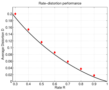
Figure 3: Plot of rate versus distortion, comparing the Shannon limit (solid line) and empirical performance using LDGM codes with blocklength $n=10,000$. Each diamond is the average distortion over 15 trials.

There remain various open questions suggested by this work. For instance, an important direction is developing methods for optimizing LDGM codes, and the choice of parameters in our extended MRFs for source encoding. An important practical issue is to investigate the tradeoff between the conservativeness of the decimation procedure (i.e., computation time) versus quality of source encoding. Finally, the limiting rate-distortion performance of LDGM codes is a theoretical question that (to the best of our knowledge) remains open.

References

- [1] M. Mézard, G. Parisi, and R. Zecchina, “Analytic and algorithmic solution of random satisfiability problems,” Science, vol. 297, 812, 2002.
- [2] E. Maneva, E. Mossel, and M. J. Wainwright, “A new look at survey propagation and its generalizations,” in Proceedings of the 16th Annual Symposium on Discrete Algorithms (SODA), 2005, pp. 1089–1098.
- [3] T. Richardson, A. Shokrollahi, and R. Urbanke, “Design of capacity-approaching irregular low-density parity check codes,” IEEE Trans. Info. Theory, vol. 47, pp. 619–637, February 2001.
- [4] G. Caire, S. Shamai, and S. Verdu, “A new data compression algorithm for sources with memory based on error-correcting codes,” in Information Theory Workshop, Paris, France, 2003, pp. 291–295.
- [5] E. Martinian and J. Yedidia, “Iterative quantization using codes on graphs,” in Allerton Conference on Control, Computing, and Communication, October 2003.
- [6] T. Murayama, “Thouless-Anderson-Palmer approach for lossy compression,” Physical Review E, vol. 69, pp. 035 105(1)–035 105(4), 2004.
- [7] M. Mézard, January 2005, personal communication, Sante Fe Coding Workshop.
- [8] D. Battaglia, A. Braunstein, J. Chavas, and R. Zecchina, “Source coding by efficient selection of ground states,” Tech. Rep., 2004, arXiv:cond-mat/0412652 v1.
- [9] M. Mézard, F. Ricci-Tersenghi, and R. Zecchina, “Alternative solutions to diluted p-spin models and XORSAT problems,” Jour. of Statistical Physics, vol. 111, p. 105, 2002.