Layered Orthogonal Lattice Detector for Two Transmit Antenna Communications

Abstract

A novel detector for multiple-input multiple-output (MIMO) communications is presented. The algorithm belongs to the class of the lattice detectors, i.e. it finds a reduced complexity solution to the problem of finding the closest vector to the received observations. The algorithm achieves optimal maximum-likelihood (ML) performance in case of two transmit antennas, at the same time keeping a complexity much lower than the exhaustive search-based ML detection technique. Also, differently from the state-of-art lattice detector (namely sphere decoder), the proposed algorithm is suitable for a highly parallel hardware architecture and for a reliable bit soft-output information generation, thus making it a promising option for real-time high-data rate transmission.

1 Introduction

Wireless transmission through multiple antennas, also referred to as MIMO (Multiple-Input Multiple-Output), currently enjoys great popularity because of the demand of high data rate communication from multimedia services.

In MIMO fading channels ML detection is desirable to achieve high-performance, as this is the optimal detection technique in presence of additive Gaussian noise. ML detection involves an exhaustive search over all the possible sequences of digitally modulated symbols, which grows exponentially as the number of transmit antennas. Because of their reduced complexity, sub-optimal linear detectors like Zero-Forcing (ZF) or Minimum Mean Square Error (MMSE) [1] are widely employed in wireless communications. Such schemes yield a low spatial diversity order: for a MIMO system with $L_{t}$ transmit and $L_{r}$ receive antennas this is equal to $L_{r}-L_{t}+1$, as opposed to $L_{r}$ for ML [2]. ZF and MMSE have also been proposed in combination with Interference Cancellation (IC) techniques [3]. However the performance of such nonlinear detectors is better than linear detectors but does not always give near-ML performance.

Lattice decoding algorithms, like sphere decoder (SD) [4], have been proposed for systems whose input-output relation can be represented as a real-domain linear model

$$\textbf{y}_{r}=\textbf{Bx}_{r}+\textbf{n}_{r}$$ (1)

where if $n=2L_{r}$ and $m=2L_{t}$, the channel output vector $\textbf{y}\in R^{n}$, the input vector $\textbf{x}\in R^{m}$ is carved from a discrete finite set of values and B is a $n$ x $m$ real matrix representing the channel mapping of the transmit codebook into a received lattice corrupted by the Gaussian noise $\textbf{n}\in R^{n}$; B is also referred to as the lattice generator matrix. SD can attain ML performances with significant reduced complexity. The lattice formulation for MIMO wireless systems was described in [5] in case of QAM digitally modulated transmitted symbols; in that case a system equation in the form (1) can be derived.

Besides SD, to our knowledge the class of ML-approaching algorithms is quite limited. Other examples include the reduced search set presented in [8], which does not yield good performance below $10^{-4}BER$, or the approximate method [9], which entails high complexity; also, no performance results are reported for a constellation size larger than QPSK.

The SD algorithm converges at the ML solution while searching a much lower number of lattice points than the exhaustive search required by a ”brute-force” ML detector. However, it presents a number of disadvantages; most important are:

1. It is an inherently serial detector and thus is not suitable for a parallel implementation.

2. Parameter sensitivity. The number of lattice points to be searched is variable and sensitive to many parameters like the choice of the initial radius; the signal to noise ratio (SNR); the (fading) channel conditions. This means it could be unsuitable for applications requiring a real-time response in data communications.

3. Bit soft output generation. In [11] the idea of building a ”candidate list” of sequences to compute the bit log-likelihood ratios (LLR) was discussed. Unfortunately the optimal size of such a list is a function of the system parameters and can still be very high (thousands of lattice points) for practical applications.

In this paper, we propose a novel layered orthogonal lattice detector (LORD) for two transmit antenna MIMO systems, which achieves ML performance in case of hard-output demodulation and optimally computes bit LLRs when soft output information is generated. Similarly to SD, LORD consists of three different stages, namely a lattice formulation, different from the one introduced in [5] and typically used by SD; the preprocessing of the channel matrix, which is basically an efficient way to perform a QR decomposition; and finally the lattice search, which finds an optimal solution to the closest vector problem [6], given the observations. The innovative concept, compared to SD, is that the search of the lattice points can be made in a parallel fashion, and fully deterministic. The number of lattice points to be searched is well below the exhaustive search ML algorithm, and for soft output generation is linear in the number of transmit antennas.

The paper is organized as follows. In Section 2 we introduce the system notation used throughout the paper and describe the lattice representation for LORD. In Section 3 the preprocessing algorithm of the lattice matrix is described. Section 4 details the reduced complexity ML demodulation technique. Its principles lead to the formulation of the optimal max-log bit LLR derivation, explained in Section 5. Section 6 shows the performance results obtained applying LORD to a BICM system and flat Rayleigh fading channel. Finally, Section 7 concludes the paper.

2 System Notation and Lattice Formulation

The scenario considered in this document is a linear MIMO communication system with $L_{t}=2$ transmit and $L_{r}$ receive antennas and frequency nonselective fading channel. The information symbol vector x $=(X_{1}\,\,X_{2})^{T}$, where $X_{j},\,j=1,\,2$ is a complex symbol belonging to a given quadrature-amplitude modulation (QAM) or phase-shift keying (PSK) constellation, is distributed among the two transmit antennas and synchronously transmitted. The signal received at each antenna is therefore a superposition of the two transmitted signals corrupted by multiplicative fading and additive white Gaussian noise (AWGN). The output of the matched filters to the pulse shape at each receive antenna can be written in matrix notation as:

$$\textbf{y}=\sqrt{\frac{E_{s}}{2}}\,\textbf{Hx}+\textbf{n}$$ (2)

where $E_{s}$ is the energy per transmitted symbol (under the hypothesis that the average constellation energy is $E[|X_{j}|^{2}]=1$); the entries of the $L_{r}$ x 2 channel matrix H, $H_{ji}$, represent the complex path gains from transmit antenna $i$ to receive antenna $j$; y $=(Y_{1}\,\ldots Y_{L_{r}})^{T}$ and n $=(N_{1}\,\ldots N_{L_{r}})^{T}$ are the $L_{r}$ x 1 complex received signal and AWGN sample vectors respectively. The complex path gains are samples of zero mean Gaussian random variables (RVs) with variance $\sigma^{2}_{H}=0.5$ per real dimension. Fading processes for different transmit and receive antenna pairs are assumed to be independent. We assume independent noise at each receive antennas, samples of independent circularly symmetric zero-mean complex Gaussian RVs with variance $N_{0}/2$ per dimension.

In the remainder of this paper we will always assume $L_{t}=2$. It will prove useful later to use the notation

$$\textbf{y}=\sqrt{\frac{E_{s}}{2}}\,\left[\textbf{h}_{c1}\,\textbf{h}_{c2}\right]\,\textbf{x}+\textbf{n}$$ (3)

where $\textbf{h}_{ci}$ is the complex gain vector from the $i^{th}$ transmit antenna to the receive antennas.

The present paper deals with a simplified yet optimal method to estimate the transmit sequence x, i.e. it solves the ML detection problem:

$$\tilde{\textbf{x}}=\arg\min_{\mathbf{x}}\|\textbf{y}-\sqrt{\frac{E_{s}}{2}}\,\textbf{Hx}\|^{2}$$ (4)

The algorithms deals only with real quantities, i.e. the in-phase (I) and quadrature-phase (Q) components of the complex quantities in (2). To this end a suitable lattice representation of the MIMO system is defined:

$$\textbf{x}_{r} = \left[X_{1,I},\ X_{1,Q},\ X_{2,I},\ X_{2,Q}\right]^{T}=\left[x_{1},\ldots,\,x_{4}\right]^{T}$$ (5)

$$\textbf{y}_{r} = \left[Y_{1,I},\ Y_{1,Q},\ldots\ ,\,Y_{L_{r},I},\ Y_{L_{r},Q}\right]^{T}$$ (6)

$$\textbf{n}_{r} = \left[N_{1,I},\ N_{1,Q},\ldots\ ,\,N_{L_{r},I},\ N_{L_{r},Q}\right]^{T}$$ (7)

Then (3) can be re-written as:

$$\textbf{y}_{r}=\sqrt{\frac{E_{s}}{2}}\,\textbf{H}_{r}\textbf{x}_{r}+\textbf{n}_{r}=\sqrt{\frac{E_{s}}{2}}\,\left[\begin{array}[]{ccc}\textbf{h}_{1},\ldots,\,\textbf{h}_{4}\end{array}\right]\,\textbf{x}_{r}+\textbf{n}_{r}$$ (8)

$\textbf{H}_{r}$ is the real channel matrix, which acts as the lattice generator matrix - cfr. (1). Each pair of columns ($\textbf{h}_{2k-1},\ \textbf{h}_{2k}$), $k=\{1,2\}$, has the form:

$$\textbf{h}_{2k-1} = \left[\Re{\left[H_{1k}\right]},\,\Im{\left[H_{1k}\right]},\ \Re{\left[H_{2k}\right]},\,\Im{\left[H_{2k}\right]},\ldots,\,\Re{\left[H_{L_{r}k}\right]},\,\Im{\left[H_{L_{r}k}\right]}\right]^{T}$$ (9)

$$\textbf{h}_{2k} = \left[-\Im{\left[H_{1k}\right]},\,\Re{\left[H_{1k}\right]},\ -\Im{\left[H_{2k}\right]},\,\Re{\left[H_{2k}\right]},\ldots,\,-\Im{\left[H_{L_{r}k}\right]},\,\Re{\left[H_{L_{r}k}\right]}\right]^{T}$$ (10)

It should be noted that this ordering is slightly different than the ordering used in the lattice search literature for multiple antenna communications. This change in ordering greatly impacts the complexity and architecture of the ML demodulator.

3 The Preprocessing Algorithm

This section describes an efficient way to preprocess $\textbf{H}_{r}$, defined in (8)-(10). It should be understood that a standard QR decomposition could be applied without impairing the detection algorithm; the algorithm described below however is more efficient as particular care is taken to avoid performing unnecessary operations (e.g., vector normalization, implying a real division and square root). Specifically for $L_{r}\geq 2$ there is an $2L_{t}\times 2L_{r}$ orthogonal matrix

$${\bf Q}=\left[\begin{array}[]{ccc}\textbf{h}_{1}\quad\textbf{h}_{2}\quad\textbf{q}_{3}\quad\textbf{q}_{4}\end{array}\right]$$ (11)

where

$$\textbf{q}_{3} = \|\textbf{h}_{1}\|^{2}\textbf{h}_{3}-(\textbf{h}_{1}^{T}\textbf{h}_{3})\textbf{h}_{1}-(\textbf{h}_{2}^{T}\textbf{h}_{3})\textbf{h}_{2}$$ (12)

$$\textbf{q}_{4} = \|\textbf{h}_{1}\|^{2}\textbf{h}_{4}-(\textbf{h}_{1}^{T}\textbf{h}_{4})\textbf{h}_{1}-(\textbf{h}_{2}^{T}\textbf{h}_{4})\textbf{h}_{2}$$ (13)

such that

$${\bf Q}^{T}{\bf Q}=\mbox{diag}\left[\left\|\textbf{h}_{1}\right\|^{2},\left\|\textbf{h}_{1}\right\|^{2},\left\|\textbf{q}_{3}\right\|^{2},\left\|\textbf{q}_{3}\right\|^{2}\right].$$ (14)

It should be noted that

$$\left\|\textbf{q}_{3}\right\|^{2}=\left\|\textbf{h}_{1}\right\|^{2}\left(\left\|\textbf{h}_{3}\right\|^{2}\left\|\textbf{h}_{1}\right\|^{2}-\left(\textbf{h}_{1}^{T}\textbf{h}_{3}\right)^{2}-\left(\textbf{h}_{2}^{T}\textbf{h}_{3}\right)^{2}\right)=\left\|\textbf{h}_{1}\right\|^{2}r_{3}$$ (15)

where

$$r_{3}=\left\|\textbf{h}_{3}\right\|^{2}\left\|\textbf{h}_{1}\right\|^{2}-\left(\textbf{h}_{1}^{T}\textbf{h}_{3}\right)^{2}-\left(\textbf{h}_{2}^{T}\textbf{h}_{3}\right)^{2}.$$ (16)

There is a $2L_{t}\times 2L_{t}$ upper triangular matrix

$${\bf R}=\left[\begin{array}[]{cccc}1&0&\textbf{h}_{1}^{T}\textbf{h}_{3}&\textbf{h}_{1}^{T}\textbf{h}_{4}\\ 0&1&\textbf{h}_{2}^{T}\textbf{h}_{3}&\textbf{h}_{2}^{T}\textbf{h}_{4}\\ 0&0&1&0\\ 0&0&0&1\end{array}\right]$$ (17)

There is a $2L_{t}\times 2L_{t}$ diagonal matrix

$${\bf\Lambda}_{q}=\mbox{diag}\left[1,1,\ \left\|\textbf{h}_{1}\right\|^{-2},\left\|\textbf{h}_{1}\right\|^{-2}\right].$$ (18)

These three matrices are related to the original real channel matrix as

$${\bf H}_{r}={\bf Q}{\bf R}{\bf\Lambda}_{q}.$$ (19)

It should be noted that if $L_{r}=1$ then the bottom two rows of ${\bf R}$ will be eliminated but the same general form will hold for the top two rows.

Because of this structure the detection problem on the MIMO channel can be transformed into a structure suitable for lattice search algorithms. To this end note that the $4\times 1$ vector

$$\tilde{\textbf{y}}={\bf Q}^{T}\textbf{y}_{r}=\sqrt{\frac{E_{s}}{2}}\,{\bf\tilde{R}}\textbf{x}_{r}+{\bf Q}^{T}\textbf{n}_{r}=\sqrt{\frac{E_{s}}{2}}\,\tilde{{\bf R}}\textbf{x}_{r}+\tilde{\textbf{n}}$$ (20)

where

$$\tilde{{\bf R}}={\bf Q}^{T}{\bf Q}{\bf R}{\bf\Lambda}_{q}=\left[\begin{array}[]{cccc}\left\|\textbf{h}_{1}\right\|^{2}&0&\textbf{h}_{1}^{T}\textbf{h}_{3}&\textbf{h}_{1}^{T}\textbf{h}_{4}\\ 0&\left\|\textbf{h}_{1}\right\|^{2}&\textbf{h}_{2}^{T}\textbf{h}_{3}&\textbf{h}_{2}^{T}\textbf{h}_{4}\\ 0&0&r_{3}&0\\ 0&0&0&r_{3}\end{array}\right].$$ (21)

The noise vector in the triangular model still has independent components but the components have unequal variances, i.e.,

$${\bf R}_{\tilde{n}}=E\left[\tilde{\textbf{n}}\tilde{\textbf{n}}^{T}\right]=\frac{N_{0}}{2}\,\mbox{diag}\left[\left\|\textbf{h}_{1}\right\|^{2},\ \left\|\textbf{h}_{1}\right\|^{2},\ \left\|\textbf{h}_{1}\right\|^{2}r_{3},\ \left\|\textbf{h}_{1}\right\|^{2}r_{3}\right].$$ (22)

The interesting characteristic of the model formulation in this manner is that each of the I and Q components of each transmitted signal are broken into orthogonal dimensions and can be searched in an independent fashion.

All parameters needed in this triangularized model are a function of eight variables. Four of the variables are functions of the channel only, i.e.,

$$\sigma^{2}_{1}=\left\|\textbf{h}_{1}\right\|^{2}\qquad\sigma^{2}_{2}=\left\|\textbf{h}_{3}\right\|^{2}\qquad s_{1}=\textbf{h}_{1}^{T}\textbf{h}_{3}\qquad s_{2}=\textbf{h}_{1}^{T}\textbf{h}_{4}.$$ (23)

and four are functions of the channel and the observations, i.e.,

$$V_{1}=\textbf{h}_{1}^{T}\textbf{y}_{r}\qquad V_{2}=\textbf{h}_{2}^{T}\textbf{y}_{r}\qquad V_{3}=\textbf{h}_{3}^{T}\textbf{y}_{r}\qquad V_{4}=\textbf{h}_{4}^{T}\textbf{y}_{r}.$$ (24)

It should be noted that $\left\|\textbf{h}_{1}\right\|^{2}=\left\|\textbf{h}_{2}\right\|^{2}$, $\left\|\textbf{h}_{3}\right\|^{2}=\left\|\textbf{h}_{4}\right\|^{2}$, $\textbf{h}_{1}^{T}\textbf{h}_{3}=\textbf{h}_{2}^{T}\textbf{h}_{4}$, and that $\textbf{h}_{1}^{T}\textbf{h}_{4}=-\textbf{h}_{2}^{T}\textbf{h}_{3}$. These two equalities imply that the $2\times 2$ matrix in the upper right corner of ${\bf\tilde{R}}$ is a rotation matrix. Specifically the required results for the upper triangular formulation is

$$\tilde{\textbf{y}}=\left[\begin{array}[]{c}\tilde{y_{1}}\\ \tilde{y_{2}}\\ \tilde{y_{3}}\\ \tilde{y_{4}}\end{array}\right]=\left[\begin{array}[]{c}V_{1}\\ V_{2}\\ \sigma^{2}_{1}V_{3}-s_{1}V_{1}+s_{2}V_{2}\\ \sigma^{2}_{1}V_{4}-s_{2}V_{1}-s_{1}V_{2}\end{array}\right]\quad{\bf\tilde{R}}=\left[\begin{array}[]{cccc}\sigma^{2}_{1}&0&s_{1}&s_{2}\\ 0&\sigma^{2}_{1}&-s_{2}&s_{1}\\ 0&0&\sigma^{2}_{1}\sigma^{2}_{2}-s_{1}^{2}-s_{2}^{2}&0\\ 0&0&0&\sigma^{2}_{1}\sigma^{2}_{2}-s_{1}^{2}-s_{2}^{2}\end{array}\right].$$ (25)

This formulation greatly simplifies the lattice search formulation and results in a preprocessing complexity that is $O(16L_{r})$.

As it will prove useful when dealing with soft output generation, shifting the ordering of the transmit antennas will result in a similar model. When the order of transmit antennas is reversed the model becomes

$$\tilde{\textbf{y}}_{s}=\left[\begin{array}[]{c}\tilde{y_{s1}}\\ \tilde{y_{s2}}\\ \tilde{y_{s3}}\\ \tilde{y_{s4}}\end{array}\right]=\left[\begin{array}[]{c}V_{3}\\ V_{4}\\ \sigma^{2}_{2}V_{1}-s_{1}V_{3}-s_{2}V_{4}\\ \sigma^{2}_{2}V_{2}+s_{2}V_{3}-s_{1}V_{4}\end{array}\right]\,{\bf\tilde{R}}_{s}=\left[\begin{array}[]{cccc}\sigma^{2}_{2}&0&s_{1}&-s_{2}\\ 0&\sigma^{2}_{2}&s_{2}&s_{1}\\ 0&0&\sigma^{2}_{1}\sigma^{2}_{2}-s_{1}^{2}-s_{2}^{2}&0\\ 0&0&0&\sigma^{2}_{1}\sigma^{2}_{2}-s_{1}^{2}-s_{2}^{2}\end{array}\right]$$ (26)

4 ML Demodulation

In this section we describe how the system equations defined in Section 4 lead to a simplified yet optimal ML demodulation. Consider a PSK or QAM constellation of size S. For the sake of conciseness, the discussion here will assume that $(M^{2})$-QAM modulation is used on each antenna, but the derivation is valid - with straightforward generalizations - for any complex constellation. The optimum ML word demodulator (4) would have to compute the ML metric for $M^{2L_{t}}$ constellation points and has a complexity $O(M^{4})$ for $L_{t}=2$.

The notation used in the sequel is that $\Omega_{x}$ will refer to the M-PAM constellation for each real dimension. Given the formulation in (20)-(25) and neglecting scalar energy normalization factors for simplicity, the ML decision metric becomes

$$T(\textbf{x}_{r}) = -\frac{\left(\tilde{y}_{1}-\sigma^{2}_{1}x_{1}-s_{1}x_{3}-s_{2}x_{4}\right)^{2}}{\sigma^{2}_{1}}-\frac{\left(\tilde{y}_{2}-\sigma^{2}_{1}x_{2}+s_{2}x_{3}-s_{1}x_{4}\right)^{2}}{\sigma^{2}_{1}}$$ (27)

$$-\frac{\left(\tilde{y}_{3}-r_{3}x_{3}\right)^{2}}{\sigma^{2}_{1}r_{3}}-\frac{\left(\tilde{y}_{4}-r_{3}x_{4}\right)^{2}}{\sigma^{2}_{1}r_{3}}$$

The ML demodulator finds the maximum value of the metric over all possible values of the sequence $\textbf{x}_{r}$. This search can be greatly simplified by noting for given values of $x_{3}$ and $x_{4}$ the maximum likelihood metric reduces to

$$T(\textbf{x}_{r})=-\frac{\left(\tilde{y}_{1}-\sigma^{2}_{1}x_{1}-C_{1}(x_{3},x_{4})\right)^{2}}{\sigma^{2}_{1}}-\frac{\left(\tilde{y}_{2}-\sigma^{2}_{1}x_{2}-C_{2}(x_{3},x_{4})\right)^{2}}{\sigma^{2}_{1}}-C_{3}(x_{3},x_{4})$$ (28)

where

$$C_{1}(x_{3},x_{4})=s_{1}x_{3}+s_{2}x_{4}\qquad C_{2}(x_{3},x_{4})=-s_{2}x_{3}+s_{1}x_{4}\qquad C_{3}(x_{3},x_{4})\geq 0$$ (29)

It is clear from examining (28) that due to the orthogonality of the problem formulation the conditional ML decision on $x_{1}$ and $x_{2}$ can immediately be made by a simple threshold test, i.e.,

$$\hat{x}_{1}(x_{3},x_{4})=\mbox{round}\left(\frac{\tilde{y}_{1}-C_{1}(x_{3},x_{4})}{\sigma^{2}_{1}}\right),\quad\hat{x}_{2}(x_{3},x_{4})=\mbox{round}\left(\frac{\tilde{y}_{2}-C_{2}(x_{3},x_{4})}{\sigma^{2}_{1}}\right).$$ (30)

The round operation is a simple slicing operation to the constellation elements of $\Omega_{x}$. The final ML estimate is then given as

$$\left\{\hat{x_{1}}(\hat{x_{3}},\hat{x_{4}}),\hat{x_{2}}(\hat{x_{3}},\hat{x_{4}}),\hat{x_{3}},\hat{x_{4}}\right\}=\arg\stackrel{{\scriptstyle\textstyle\max}}{{\scriptstyle x_{3},x_{4}\in\Omega_{x}^{2}}}\left\{-\frac{\left(\tilde{y}_{1}-\sigma^{2}_{1}\hat{x}_{1}(x_{3},x_{4})-C_{1}(x_{3},x_{4})\right)^{2}}{\sigma^{2}_{1}}\right.$$

$$-\left.\frac{\left(\tilde{y}_{2}-\sigma^{2}_{1}\hat{x}_{2}(x_{3},x_{4})-C_{2}(x_{3},x_{4})\right)^{2}}{\sigma^{2}_{1}}-C_{3}(x_{3},x_{4})\right\}$$ (31)

This implies that the number of points that has to be searched in this formulation to find the true ML estimator is $M^{2}$ (with two slicing operations per searched point) and not $M^{4}$. This is a significant saving in complexity.

Examining (30) and (4) shows this reduced complexity ML demodulation is a direct consequence of the reordered lattice formulation. Recall each group of two rows in the model correspond to a transmit antenna. Equation (30) shows that at the top of the triangularized model the decisions for the first transmit antenna can be made independently for the I and the Q modulation. This was not true for the traditional lattice formulation [5] as after the triangularization the higher rows become dependent on all the lower layers of the transmit modulation. Retaining this orthogonalization greatly simplifies the optimal search and has important implications for suboptimal searches. Secondly this orthogonalization also greatly facilitates parallel searches, solving one of SD drawbacks, i.e. the fact that the search must be performed in a recursive fashion.

5 LLR generation

The problem is first here recalled for complex-domain system (2). Consider the information symbol vector x $=(X_{1}\,\,X_{2})^{T}$, where $X_{j},\,j=1,\,2$ is a complex symbol belonging to a given $M^{2}$-QAM constellation and be $M_{c}$ the number of bits per symbol. The bit soft-output information is the a-posteriori probability (APP) ratio of the bit $b_{k}$, $k=1,\ldots,2M_{c}\,$, conditioned on the received channel symbol vector y; that is often expressed in the logarithmic domain (log-likelihood ratio, LLR) as:

$$L(b_{k}|\textbf{y})=\ln{\frac{P(b_{k}=1|\textbf{y})}{P(b_{k}=0|\textbf{y})}}=\ln{\frac{\displaystyle\sum_{{\bf x}\in S(k)^{+}}P(\textbf{y}|\textbf{x})P_{a}(\textbf{x})}{\displaystyle\sum_{{\bf x}\in S(k)^{-}}P(\textbf{y}|\textbf{x})P_{a}(\textbf{x})}}$$ (32)

where $S(k)^{+}$ is the set of $2^{2Mc-1}$ bit sequences having $b_{k}=1$, and similarly $S(k)^{-}$ is the set of bit sequences having $b_{k}=0$; $P_{a}({\bf x})$ represent the a-priori probabilities of x, which can be neglected in case of equiprobable transmit symbols, as it is the case of this paper. In the general case, the likelihood function $\displaystyle P(\textbf{y}|\textbf{x})$ can be derived from (2):

$$P(\textbf{y}|\textbf{x})\propto\exp{\left[-\frac{1}{2\sigma^{2}}\|\textbf{y}-\sqrt{\frac{E_{s}}{2}}\textbf{Hx}\|^{2}\right]}=\exp{\left[-D(\textbf{x})\right]}$$ (33)

where $\sigma^{2}=N_{0}/2$ and $D(\textbf{x})$ is the Euclidean distance term. The summation of exponentials involved in (32) is often approximated according to the following so-called max-log approximation:

$$\ln{\sum_{{\bf x}\in S(k)^{+}}\exp{\left[-D({\bf x})\right]}}\approx\ln{\max_{{\bf x}\in S(k)^{+}}{\exp{\left[-D({\bf x})\right]}}}=-\min_{{\bf x}\in S(k)^{+}}{D({\bf x})}$$ (34)

Alternatively, it is possible to exactly compute (32) through the “Jacobian logarithm” or $\max^{*}$ function

$$\textrm{jacln}(a,b):=\ln{\left[\exp{(a)}+\exp{(b)}\right]}=\max{(a,b)}+\ln{\left[1+\exp{(-|a-b|)}\right]}.$$ (35)

Simulations in [10] show that the performance degradation due to max-log approximation is generally very small compared to the use of $\max^{*}$ function. Using (34), (32) can then be written as:

$$L(b_{k}|\textbf{y})\approx\min_{{\bf x}\in S(k)^{-}}{D(\textbf{x})}-\min_{{\bf x}\in S(k)^{+}}{D(\textbf{x})}$$ (36)

In the sequel we will show how LORD can provide an exact computation of (36) but with a much lower complexity than exhaustive search-ML. The computation of (36) requires identification of the most likely lattice point with $b_{k}=1$ and the most likely lattice point with $b_{k}=0$ for each bit index $k=1,\ldots,2M_{c}$. The problem in the case of the SD algorithm is clearly stated in [11]. By definition, one of the two sequences is the (optimum) hard-decision ML solution of (4). However, using SD, there is no guarantee that the other sequence is one of the valid lattice points found by SD during the process of the lattice search.

LORD does not have this problem generating LLRs. To show this let us consider the bits corresponding to the complex symbol $X_{2}$ in the symbol sequence x $=(X_{1}\,\,X_{2})^{T}$. After the lattice representation is derived, from (20) and (27) the likelihood function $\displaystyle P(\tilde{\textbf{y}}|\textbf{x}_{r})$ is given by:

$$P(\tilde{\textbf{y}}|\textbf{x}_{r})=\exp\left[-|T(\textbf{x}_{r})|\right].$$ (37)

where $T(\textbf{x}_{r})$ is defined in (27). Using arguments similar to those that led to the simplified ML demodulation (28)-(30), one can easily prove that the two sequences needed for every bit in $X_{2}$ are certainly found minimizing (27) over the possible $M^{2}$ values of ($x_{3},\,x_{4}$) and performing a simple slicing operation to the constellation elements of $\Omega_{x}$; thus the desired couples ($x_{1},\,x_{2}$) are uniquely determined for every ($x_{3},\,x_{4}$). Equation (32) can be then written as:

$$L(b_{2,k}|\tilde{\textbf{y}})\approx\min_{x_{3},x_{4}\in S(k)_{2}^{-}}{T(\textbf{x}_{r})}-\min_{x_{3},x_{4}\in S(k)_{2}^{+}}{T(\textbf{x}_{r})}$$ (38)

where $b_{2,k}$ are the bits corresponding to $X_{2}$, $k=1,\ldots,M_{c}$, and $S(k)_{2}^{+}$ ($S(k)_{2}^{-}$) are the set of $2^{M_{c}-1}$ bit sequences having $b_{2,k}=1$ ($b_{2,k}=0$).

The computation of the LLRs for the bits corresponding to symbols in ${x_{1},x_{2}}$ can be obtain by a simple reordering of the model and a repeating of the LORD processing. To this end denote $\textbf{x}_{s}=\left[x_{3}\,x_{4}\,x_{1}\,x_{2}\right]$ as the reordered real modulation symbols, then the LLR can be given as

$$L(b_{1,k}|\tilde{\textbf{y}_{s}})\approx\min_{x_{1},x_{2}\in S(k)_{1}^{-}}{T^{\prime}(\textbf{x}_{s})}-\min_{x_{1},x_{2}\in S(k)_{1}^{+}}{T^{\prime}(\textbf{x}_{s})}$$ (39)

where $b_{1,k}$ are the bits corresponding to $X_{1}$, $k=1,\ldots,M_{c}$, $S(k)_{1}^{+}$ ($S(k)_{1}^{-}$) are the set of $2^{M_{c}-1}$ bit sequences having $b_{1,k}=1$ ($b_{1,k}=0$). The reordered ML decision metric becomes

$$T^{\prime}(\textbf{x}_{s}) = -\frac{\left(\tilde{y}_{s1}-\sigma^{2}_{2}x_{3}-s_{1}x_{1}+s_{2}x_{2}\right)^{2}}{\sigma^{2}_{2}}-\frac{\left(\tilde{y}_{s2}-\sigma^{2}_{2}x_{4}-s_{2}x_{1}-s_{1}x_{2}\right)^{2}}{\sigma^{2}_{2}}$$ (40)

$$-\frac{\left(\tilde{y}_{s3}-r_{3}x_{1}\right)^{2}}{\sigma^{2}_{2}r_{3}}-\frac{\left(\tilde{y}_{s4}-r_{3}x_{2}\right)^{2}}{\sigma^{2}_{2}r_{3}}$$

in a direct analogy to (26). By comparing (26) and (25), it should be clear that computing the processing required by the reordered sequence involves a low amount of extra-complexity. Besides, the LLR computation for the bits corresponding to symbols $X_{1}$ and $X_{2}$ can be carried out in a parallel fashion. Thus, we have derived an exact Max-log bit LLR computation using two layer orderings and an overall lattice search over $2M^{2}$ sequences instead of $M^{4}$ as would be required by the exhaustive search-based ML algorithm.

6 Performance results

In this section two examples are presented with the corresponding performance evaluated by simulation. The examples will be limited to frequency flat and time flat fading for simplicity but this does not represent a limit on how LORD can be applied in MIMO detection. The first example is an uncoded $L_{t}=2$ system using 64QAM modulation. The maximum likelihood detection word error probability performance in spatially white Rayleigh fading is shown in Fig. 1. The ML performance is compared to the well understood zero forcing (ZF) detector. The advantage of ML detection versus linear detection in terms of diversity is obvious from these plots.

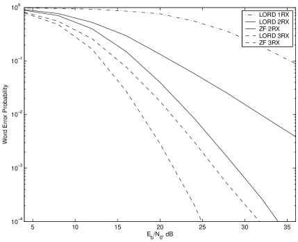
a) Word error probability.

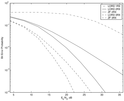
b) Bit error probability.

Figure 1: The decoding performance for uncoded MIMO transmission. $L_{t}=2$ and 12 bits per channel use.

A second system consists of a bit interleaved coded modulation (BICM) with a frame size of 144 coded bits using 64QAM modulation on each antenna. The interleaver used was a $12\times 12$ block interleaver so that each adjacent bit could be permuted to a different antenna and different significant bit on the QAM modulation while being on different time slots. The convolutional code is the standard 64-state rate 1/2 binary convolutional code with octal generators (133, 171). The performance is shown in Fig. 2 for $L_{t}=2$, $L_{r}=2$, and spatially white Rayleigh fading for both hard and max-log inner bit metric generation. Clearly this figure demonstrates LORD is a system that can exactly compute the max-log LLR at a low complexity when used in a concatenated MIMO coded modulation.

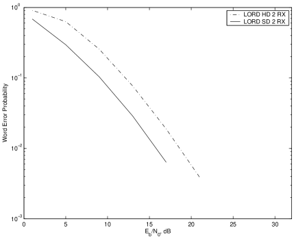
a) Word error probability.

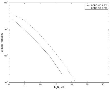
b) Bit error probability.

Figure 2: The BICM decoding performance. $L_{t}=2$, $L_{R}=2$ and 6 bits per channel use.

7 Conclusion

We have presented a novel lattice search-based MIMO detection algorithm for two transmit antennas, characterized by a low preprocessing complexity, that achieves optimal ML demodulation with a complexity of the order of $S$, if $S$ is the constellation size. Also, the algorithm is able to generate optimal Max-log bit LLRs using a parallel lattice search over $2S$ transmit sequences.

To our knowledge no ML-approaching detection technique, among those proposed so far, is able to generate a low complexity optimal bit soft output information and easily be suitable for a parallel hardware implementation. LORD provides all these desirable features and thus represents a significant improvement over the state of the art in this field.

References

- [1] P. W. Wolniansky et al., “V-BLAST: An Architecture for Realizing Very High Data Rates Over the Rich-Scattering Wireless Channel” , invited paper, Proc. ISSSE-98, Pisa, Italy, Sept. 1998.
- [2] Van Nee, Van Zelst, “Maximum likelihood decoding in a space division multiplexing system,” Awater, Proc. of IEEE Vehicular Techn. Conf. 2000, vol. 1, 6-10, 2000.
- [3] G. J. Foschini et al., “Simplified Processing for High Spectral Efficiency Wireless Communications employing multi-element arrays”, IEEE Journal on Selected Areas in Communications, vol. 17, no. 11, pp. 1841-1852, Nov. 1999.
- [4] E. Viterbo, J. Boutros, “A Universal Lattice Code Decoder for Fading Channels”, IEEE Trans. on Information Theory, Vol. 45, No. 5, July 1999.
- [5] M. O. Damen et al., “Lattice codes decoder for space-time codes”, Communication Letters, Vol. 4, pp. 161-163, May 2000.
- [6] E. Agrell et al., “Closest Point Search in Lattices”, IEEE Trans. on Information Theory, Vol. 48, No. 8, August 2002.
- [7] M. O. Damen, El Gamal, G. Caire, “On Maximum-Likelihood Detection and the Search for the Closest Lattice Point”, IEEE Trans. on Information Theory, Vol. 49, No. 10, October 2003.
- [8] M. Rupp et al., “Approximate ML Detection Systems with Very Low Complexity”, Proc. of ICASSP 2004, 2004.
- [9] H. Sung et al., “A Simplified Maximum Likelihood Detection Scheme for MIMO Systems”, IEEE Vehicular Techn. Conf. 2003-Fall, Vol. 1, pp 419 - 423, 2003.
- [10] P. Robertson, E. Villebrun, P. Hoeher, “A Comparison of Optimal and Sub-optimal MAP Decoding Algorithms Operating in the Log Domain Communications”, Proc. of IEEE International Conf. on Communications, Vol. 2, pp. 1009-1013, June 1995.
- [11] B. Hochwald, S. ten Brink, “Achieving Near-Capacity on a Multiple-Antenna Channel”, IEEE Trans. on Communications, Vol. 51, No. 3, March 2003.