Temporal and Spatial Data Mining with Second-Order Hidden Markov Models

Abstract

In the frame of designing a knowledge discovery system, we have developed stochastic models based on high-order hidden Markov models. These models are capable to map sequences of data into a Markov chain in which the transitions between the states depend on the n previous states according to the order of the model. We study the process of achieving information extraction from spatial and temporal data by means of an unsupervised classification. We use therefore a French national database related to the land use of a region, named Ter Uti, which describes the land use both in the spatial and temporal domain. Land-use categories (wheat, corn, forest, …) are logged every year on each site regularly spaced in the region. They constitute a temporal sequence of images in which we look for spatial and temporal dependencies.

The temporal segmentation of the data is done by means of a second-order Hidden Markov Model (HMM2) that appears to have very good capabilities to locate stationary segments, as shown in our previous work in speech recognition. The spatial classification is performed by defining a fractal scanning of the images with the help of a Hilbert-Peano curve that introduces a total order on the sites, preserving the relation of neighborhood between the sites. We show that the HMM2 performs a classification that is meaningful for the agronomists.

Spatial and temporal classification may be achieved simultaneously by means of a 2 levels HMM2 that measures the a posteriori probability to map a temporal sequence of images onto a set of hidden classes.

1 Context

Mining sequential and spatial patterns is an active area of research in artificial intelligence. One basic problem in analyzing a sequence of items is to find frequent episodes, i.e. collections of events occurring frequently together. Early in 1995, Agrawal [2, 1] proposes non-numeric algorithms for extracting regular patterns from temporal data. Conversely, we present in this paper new numerical algorithms, based on high-order stochastic models – the second-order hidden Markov models (HMM2) – capable to discover frequent sequences of events in temporal and spatial data. These algorithms were initially specified for speech recognition purposes [20] in our laboratory. We show that, with minor changes, they can extract spatial and temporal regularities that can be explained by human experts and may constitute some atoms of knowledge [11].

The HMM2’s are based on the probabilities and statistics theories. Their main advantage is the existence of unsupervised training algorithms that allow to estimate a model parameters from a corpus of observations and an initial model. Several criteria are used : the maximum likelihood criterium implemented in the well known EM algorithm  [14], the maximum a posteriori criterium [17] and the maximum mutual information criterium [5]. Rabiner [29] gives an extensive description of analytical learning methods for HMM. Other algorithms [28, 30], based on stochastic likelihood maximization and Bayesian estimation have shown interesting results. The resulting model is capable to segment each sequence in stationary and transient parts and to build up a classification of the data together with the a posteriori probability of this classification. This characteristic makes the HMM2’s appropriate to discover temporal and spatial regularities like it is shown in various areas: speech recognition [19, 22] image restoration and segmentation  [7], genetics [27, 10, 16], robotics [4], data mining [9, 33, 18], decision helping [12].

We focused our effort on two points: 1) the elaboration of a process of mining spatial and temporal dependencies aiming to the elicitation of knowledge. This process always involves an unsupervised classification of the data. 2) The specification of adequate visualization tools that give a synthetic view of the classification results to the experts who have to interpret the classes and/or specify new experiments.

In this paper, we present our methodology and give some results in the data mining of temporal and spatial data in the framework of the agricultural land use evolution. We show on various examples that the HMM2’s are powerful tools for temporal and spatial data mining. Another title of this paper could be: ”How to understand what the land use talks to us”.

This paper is organized as follows. After an introduction (section 1), Section 2 describes the models that we used for classification purposes. Section 3 describes the agricultural data and our attitude in data mining in collaboration with agronomists. The resulting tied interaction yields to the production of a free software named CarrotAge. The fourth section is the description of two major applications of CarrotAge. Section 5 is a conclusion.

2 Modeling sequence dependencies with HMM2

2.1 HMM2 definition

We define a second-order hidden Markov model by giving:

• ${\bf S}=\left\{s_{1},s_{2},\ldots,s_{N},\right\},$ a finite set of $N$ states ;

• ${\bf A}$ a matrix defining the transition probabilities between the states:

  ${\bf A}=\left(a_{ij}\right)$

  for a first order HMM (HMM1),

  ${\bf A}=\left(a_{ijk}\right)$

  for a second order HMM (HMM2) ;

• $\mathbf{b_{i}(.)}$ the distribution of observations associated to the states $s_{i}$. This distribution may be parametric, non parametric or even given by an HMM (see Figures 2 or 3.

A Markov chain is defined over a set of states – the crops in a field, or more generally the land-use categories in a place – that are unambiguously observed. The Markov chain specifies only one stochastic process, whereas in a HMM, the observation of a land-use category is not uniquely associated to a state $s_{i}$ but is rather a random variable that has a conditional density $b_{i}(.)$ that depends on the actual state $s_{i}$ [6]. There is a doubly stochastic process:

– the former is hidden from the observer and is defined on a set of states;

– the latter is visible. It produces an observation, the land-use of a parcel, at each time slot depending on the probability density function (pdf) that is defined on the state in which the Markov chain stays at time $t$. It is often said that the Markov chain governs the latter.

In this framework, we consider that the distribution of the country’s land use is a Markov chain. The crop pattern at year $t$ depends at least upon the crop pattern the year before $(t-1)$ or 2 years before $(t-2)$.

2.2 Automatic estimation of a HMM2

The estimation of an HMM1 is usually done by the Forward Backward algorithm which is related to the EM algorithm [14]. We have shown in [21] that an HMM2 can be estimated following the same way. The estimation is an iterative process starting with an initial model and a corpus of sequences of observations that the HMM2 must fit even when the insertions, deletions and substitutions of observations occur in the sequences. The very success of the HMM is based on their robustness: even when the considered data do not suit a given HMM, its use can give interesting results. The initial model has equiprobable transition probabilities and an uniform distribution in each state. At each step, the Forward-backward algorithm determines a new model in which the likelihood of the sequences of observation increases.

Hence this estimation process converges to a local maximum. Interested readers may refer to [14, 23] to find more specific details of the implementation of this algorithm.

If N is the number of states and T the sequence length, the Forward - Backward has a complexity of $\texttt{N}^{3}\times\texttt{T}$ for an HMM2.

The choice of the initial model has an influence on the final model obtained by convergence. To assess this last model, we use the Kullback-Leibler distance between the distributions associated to the states [34]. Two states that are too close are merged and the resulting model is re-trained. Agronomists do not interfere in the process of designing a specific model, but they have a central role in the interpretation of the results that the final model gives on the data.

2.3 Classification of a sequence using HMM2

The purpose of pattern recognition is to specify as much models as there are classes to recognize. As opposite to pattern recognition, we do not have the knowledge of what to recognize but rather look for something regular to extract, hence the name data mining.

In the present work, we specify one HMM in order to model, in a more simple way, the unknown behavior of a sequence. Each state captures a stationary behavior and represents a class where the observations are drawn with a known pdf. In an HMM2 the Forward-Backward algorithm computes a posteriori probability $a_{ijk}(t)$ that the Markov chain will be in state $k$ at time $t+1$ knowing that it has been in $j$ at $t$ and in $i$ at $t-1$. In an HMM1, the Forward-Backward algorithm computes a posteriori probability $a_{ij}(t)$ on a smaller period (2 years) that does not span most of land use successions (ususally 2 or 3 years, sometimes 4). In the EM procedure, the a priori transitions are calculated, at each iteration, as being the mean of the a posteriori transition probabilities calculated with the current parameters. These a posteriori probabilities can be plot as a function of time and determines a fuzzy classification in the states space. This classification can be interpreted by a domain expert who can give it a meaning. Figure 8 shows this function and its interpretation by an agronomist.

Experiments results in speech recognition [21] show that HMM2’s provide a better state occupancy modeling. In fact, the state duration in an HMM2 is governed by two parameters, i.e, the probability of entering a state only once, and the probability of visiting a state at least twice, with the latter modeled as a geometric decay. This distribution better fits a probability density of durations than the classical exponential distribution of an HMM1.

2.4 Modeling the spatial data dependencies

In the framework of image segmentation, Markov random fields (MRF) offer probabilistic models in which a local variable only directly depends on a few other neighboring variables. The estimation of a MRF and the classification of an image involve sophisticated and time consuming algorithms [15].

More recently, iterative fuzzy clustering methods have been applied on spatial data to find homogeneous regions. Ambroise and Dang [3] proposes a variant of the EM algorithm – called neighborhood EM (NEM) – to account for spatial proximity effects.

Due to the low spatial resolution of our data (see Section 3.2), we prefer to follow Benmilloud and Pieczynski [7] and to use a rough clustering method based on simple hidden Markov models. We have introduced a total order in the image by means of a fractal curve – a Hilbert-Peano curve – that scans the image preserving the relation of neighborhood between the sites. Two points that are close in the curve are neighbor in the picture. But, the opposite is not true. When a HMM specifies a segmentation of the Hilbert-Peano curve, it specifies also a region of the plane where the observations are supposed stationary and come from the distribution associated to the state. The unsupervised classification is performed by an ergodic model in which all the transitions between the states are possible (see Figure 1).

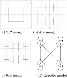
Figure 1: Definition of a total order in the plane by means of a Hilbert-Peano curve (a-c) and topology of the HMM2 used for segmentation (d). The hidden states are called: 1, 2, 3, 4.

2.5 Modeling the spatio-temporal dependencies

So far, the HMM classifies the data on the basis of their temporal or spatial features. The hidden partition is represented by the set of the HMM’s states.

We are now interested in finding how both the temporal and spatial features of a point in an image (a pixel) may interact to achieve a clustering in which the probability of the hidden partition depends in a coherent way both on the temporal and spatial features. We still keep a Bayesian point of view of the classification. We have processed our spatio-temporal data following two different ways:

1. We have a sequence of images, one per time slot. For example, a site in an image is labeled by its land-use category (see Figure 2).

2. We have one image. A site in the image is labeled by its temporal sequence of land-use categories (see Figure 3).

In both cases, the probability of the observation of a particular sequence is given by an HMM [29, 23].

In both experiments, the HMM2 that we use for image segmentation is an ergodic model (see Figure 1-d).

The data are structured as a matrix in which the rows represent the sites ordered by the Hilbert-Peano curve and the columns represent the time slots. In case (1), the sequence of images is represented by the sequence of columns. The matrix is then processed columns by columns whereas in case (2), the matrix is processed rows by rows. We define a master HMM2 whose states are in fact classical HMM2. We call them super states. The master HMM2 “generates” observations that are vectors whose probability is given by the smaller HMM2 associated to the super states. In the Figures  2 and  3, the super states of the master HMM2 are called a,b,c,… whereas the states of the HMM2 associated to the super states are called 1, 2, 3, …. In Fig. 2, the master HMM is temporal. In Fig. 2, it is spatial.

Figure 2: Each state a, b, c of the temporal master HMM2 is a ergodic HMM2 depicted Figure 1 (d)

Figure 3: Each state a, b, c, d of the master HMM2 is a temporal HMM2 with states 1, 2, 3

Our master HMM2 can be compared to those coming from the work of Saon [32, 31] that uses HMM1’s for the recognition of unconstrained handwritten words. In Saon’s work, a master HMM1 generates vectors representing columns of pixels. The sequence of columns represents the matrix in which the handwritten word is drawn. In our model whose topology is given Figure 3, the observation vector does not represent a spatial direction but is rather a time dimension. Similar models have been used in various applications. Fine [33] has defined in 1998 Hierarchical HMM for learning multi-resolution structures of natural English text. Adibi [18] uses Similar Layered HMM for analyzing and predicting the flow of packets in a network.

In our experiments, we have considered the case of one image in which the sites are labeled by a temporal sequence of land-use categories (case 2). The complexity of the Forward-backward algorithm can be assessed as follows. Assume that:

• $N_{M}$ is the number of states in the master HMM2;

• $N_{s}$, the number of states in the conventional HMM2 associated in the super states ;

• $R$ is the number of sites ;

• $T$ the number of time slots.

The Forward-backward algorithm has a complexity of $N_{M}^{3}R$ and involves the computation of $N_{M}R$ probabilities given by the conventional HMM2’s whose complexity is $N_{s}^{3}T$. Then, the overall computation stays polynomial. A very similar demonstration stands for a sequence of images (case 1).

3 HMM for mining spatio-temporal data

3.1 Introduction

One of the aspects of the data mining is to give a representation of the data that an expert can interpret. Classification is the most popular way to have a synthetic view of how the data are structured. Our purpose is to build a partition – called the hidden partition – in which the inherent noise of the data is withdrawn as much as possible. In the mining of spatio-temporal data, we are interested in extracting homogeneous classes both in temporal and spatial domains, and having a clear view of how are the transitions between these classes.

The process of data mining does not stop as soon as some regularities have been extracted but goes through several model specifications that incorporate the units of knowledge that were previously extracted from the data. In this process, the domain expert – i.e. the agronomist – plays a central role. Its task is to interpret the results of each training of various models, and to suggest new models.

Our interaction with the agronomist went through 3 steps:

1. we first have proposed to segment the data in the temporal domain with the help of a simple HMM2 (see Figure 5). A tied interaction leads to the definition of more complicated models as in Figure 6 in which the agronomists can extract and quantify information on successions of land-use categories.

2. We next have proposed to segment the whole country on a spatial basis and get the 2-D Map (Figure 7). This map helps the agronomist to distinguish the actual regions on the basis of actual successions of land-use categories.

3. Finally, we have proposed the spatio-temporal segmentation to unify the two former methods. And, we have used it to help the interpretation of satellite images (see Section 4.2).

3.2 An example of spatio-temporal data: the Ter Uti data

The Ter Uti data are collected by the French agriculture administration on the whole metropolitan territory. They represent the land use of the country on a one year basis. A first sample, done by the IGN consists to select aerial photographies to cover a part of the entire country (see Figure 4). Two levels of resolution are achieved. Each of the 3820 meshes contains 4 air photographies and a air photography covers only a square of 2 km. On each photography, a 6 by 6 grid determines 36 sites that are inquired every year in June. The fractal curve that we use for the scanning takes into account these two levels of spatial resolution. A Hilbert-Peano curve orders the 32x32 photographies that cover the region under study – ie Lorraine or Midi-Pyrénées – whereas an adapted curve (see Figure 1-c) scans the 6x6 grid of sites in the photography. The land-use category of these sites (wheat, corn, forest, …) is logged in a matrix in which the rows are the sites of the country (30000 for the Lorraine) and the columns the time slots (from 1992 to 2000). In our study, there are 49 modalities for land-use categories [8]. One Ter Uti site represents roughly 100 hectares.

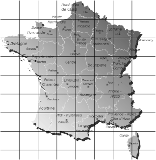
(a) the basic grid in 3820 meshes

(b) the 4 air photos in a mesh

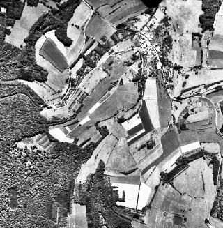
(c) the air photography and its 6x6 grid

Figure 4: Description of the Ter Uti data: 3820 meshes square France, 4 air photographies are sampled in a mesh, a 6x6 grid determines 36 sites.

3.3 Models for the temporal classification

In a first study, we have been interested in the extraction of temporal segments in which the distribution of the land-use categories is stationary. To do so, we have specified a HMM2 with 2 or 3 states with a left to right, self loops topology (see Figure 5). This means that we attempt to capture 2 or 3 periods of evolution in the land use dynamics.

state 1 state 2 state 3 pastures 0.31 pastures 0.29 wheat 0.29 wheat 0.22 wheat 0.26 pastures 0.27 barley 0.16 colza 0.14 colza 0.17 colza 0.12 barley 0.11 barley 0.12 maize 0.07 maize 0.08 maize 0.06 fallow 0.05 fallow 0.05 orchard 0.02

Figure 5: Model 1: HMM2 performing a segmentation in 3 periods in which the observations are supposed stationary. We notice the the progression of the wheat and the disappearance of the fallow lands. The hidden states are called 2, 3 and 4.

We are interested in finding 3 stationary agricultural periods. Figure 5 illustrates the results of three temporal clusterings.

Between 1992 and 1999, the country went through three different states with different distributions. The agronomists recognize the progression of wheat and the disappearance of the fallow land, two processes that are related to the EC agricultural policy.

Figure 6: Model 2: the states denoted 1, 2 and 3 are associated to a distribution of land-use categories, as opposite to the states denoted with a specific land-use category. The number of columns determine the number of time intervals (periods). A connection without arrow means a bi directional connection.

An HMM2 cannot measure the probability of a succession of three land-use categories because the states between which the transition probabilities stand represent a distribution. To tackle this problem, we have defined a specific state, called the Dirac state, whose distribution is zero except on a particular land-use category. Therefore, the transition probabilities between the Dirac states measure the probabilities between the land-use categories during a three years period. Figure 6 shows the topology of a HMM2 that has two kinds of states: Dirac states associated to the most frequent land-use categories (wheat, maize, barley, …) and container states associated to a distribution of land-use categories like it is usually done in HMM modeling framework.

3.4 Spatial classification

We did the first spatial experiment on Lorraine data: 7 images of 30000 pixels, a pixel has 49 modalities corresponding to its land-use category at a time slot (between 1992 and 1998). We trained an ergodic HMM2 (see Figure 1) with 5 states on a corpus of these 7 images. After 10 iterations the resulting model exhibits 5 distributions of land-uses:

• a state with a majority of houses, rivers, forests that follow the valleys;

• a state with a majority of forest (98 %) located in Vosges and Meuse;

• a state with a majority of pastures (30 %), forest (20 %) and fodder (6 %) located in the breeding countries;

• a state with a majority of cereals (wheat, maize, barley, …);

• a state with a majority of pastures, orchards in the bottom of valleys and mountains.

Picture 7(b) compares the segmentation performed by a HMM2 and a satellite image in which the resolution is four times higher.

(a) HMM2 classification

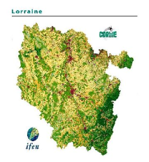
(b) Map based on satellite images

Figure 7: HMM2 classification of Lorraine Ter Uti data and comparison with a map of the same region based on satellite images (IFEN,1993).

4 Applications: CarrotAge in use

CarrotAge is a free software under a GPL licence that takes as input an array of discrete data – the rows represent the spatial sites and the columns the time slots – and builds a partition together with its a posteriori probability. This probability may be plot as a function of time and is a meaningful feature for the expert looking for stationary and transient behaviors of the data. CarrotAge is written in C++ and runs under Unix and X11R6 systems. It is now used by agronomists and geneticians [16] without any assistance of the designers.

4.1 Crop rotations in the Seine river watershed

For thirty or forty years, the hydro-system of the Seine river has been gradually degraded, regarding water quality and biological population, due to the human activities (domestic, industrial, agricultural) [25]. The nitrate contamination of cave and surface waters is mainly caused by the evolution of agricultural activities, and related to their nature and to their organization inside the river watershed. The aim of the interdisciplinary research program PIREN-Seine (Programme Interdisciplinaire de Recherche en ENvironnement sur la Seine) [26] is thus to develop a tool for forecasting water quality in the Seine river watershed, based on assumptions upon agricultural changes. In this research framework, members of the INRA team in Mirecourt analyze the agricultural activities in the watershed, their dynamics and their spatial organizations. They particularly focus on the crop (temporal) rotations that are able to explain the risk of nitrate loss.

We present an example of the approach and the results obtained on a small agricultural region from the north-east of France, the PRA (Petite Région Agricole) St-Quentinois et Laonnois.

Figure 8: Results obtained on the Ter Uti data of PRA St-Quentinois et Laonnois (Aisne, years 1992-2000).

Several models have been used in order to:

• compute the mean crop distribution in a given period, here from 1992 to 1999 (Figure 8, left) ; the states of the HMM2 are only container states. ;

• view the main annual transitions between crops (Figure 8, right) ; the states of the HMM2 are container and Dirac states (beet, wheat, pea, etc.).

These results are analyzed as follows. One can see that the main rotation heads – beet and pea – are generally followed and preceded by wheat. It is thus assumed that the rotations contain triples from the types wheat-beet-wheat or wheat-pea-wheat, and that they are 4-years rotations, either ?-wheat-beet-wheat or ?-wheat-pea-wheat. But these results do not make possible to determine the crop (denoted with ?), which is before or after these triples of crops. In Figure 8 (left) the dashed lines represent the possible transitions between the triple wheat-beet-wheat and the other crops: beet, pea, wheat, barley, colza or fallow.

Other models have been used for searching all types of crop rotations in this small region. The same analysis has been done for all small agricultural regions in the Seine watershed. The regions are then clustered according to their main crop rotations and their evolutions. These results are meaningful for specifying simulation models of nitrate loss and thus forecasting water quality in the Seine watershed.

4.2 Helping satellite images interpretation in the Midi-Pyrénées region

The first spatio temporal experiment has been done on Ter Uti data coming from the Midi-Pyrénées region.

Our approach has been used by researchers of the INRA research center in Toulouse working on the forecast of irrigation needs in the Midi-Pyrénées region (south-west of France). Usually, irrigation needs are estimated thanks to annual land-use maps based on satellite data [13]. This method is not satisfying since all data are not available at the moment when the forecast has to be done: the satellite images obtained in spring do not allow to distinguish all the crops of a given region. But if the crop rotations are known, it can help to distinguish the crops, based on the land-use map of the year before. Knowing the crop in a plot at year $n-1$, the possible crops in the same plot at year $n$ can be infered, and their number reduced thanks to the satellite images of spring.

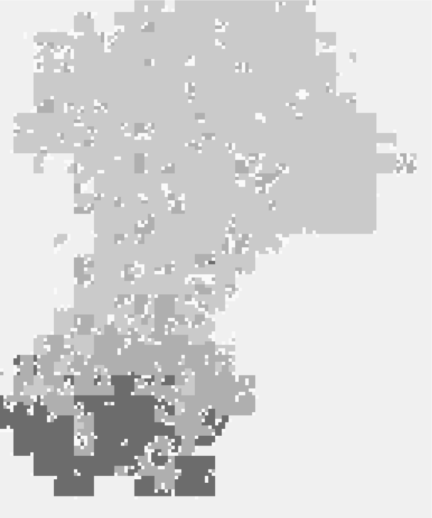
around 1992
0.099	wood + wood + wood
0.089	maize + maize + maize
0.082	pastures + pastures + pastures
0.034	wheat + sunflower + wheat
0.028	vines + vines + vines
0.026	sunflower + wheat + sunflower
0.018	fallow + fallow + fallow

around 2000
0.105	maize + maize + maize
0.099	wood + wood + wood
0.081	pastures + pastures + pastures
0.056	wheat + sunflower + wheat
0.037	sunflower + wheat + sunflower
0.027	vines + vines + vines
0.023	fallow + fallow + fallow

Figure 9: Map of the crop rotations in the Midi-Pyrénées region and evolution table in the north area (years 1992-2000).

In this framework, our approach has been used for a spatio-temporal segmentation of the Ter Uti data of the Midi-Pyrénées region. We have specified two different HMM2. The master one is an ergodic HMM2 that has to segment an image like in the former experiment. In each of the 5 states, we have defined a temporal 3 states HMM2 like in Figure 6. The territory is separated into three homogeneous areas according to the crop rotations (Figure 9): the south area (black) is mainly mountains (Pyrénées), the middle area (dark grey) is covered with alpine pastures and forests, and the north area (grey) is cultivated. The study then focused on the north area, for analyzing the evolution of the crop rotations. The table of Figure 9 shows the growing of the wheat-sunflower rotation and of the maize mono-culture. Eventually, the transition probabilities between crops (Dirac states) have been computed for the ten years where Ter Uti data were available. These transition probabilities have then been used with a land-use map of the year $n-1$ and an April satellite image in the year $n$, in order to estimate the land-use map of the year. This estimation is then evaluated with a land-use map of the year built a posteriori [24].

In this example, the models defined for spatial and temporal segmentation have been used in a complementary way. The first ones allow to define homogeneous stable areas regarding the crop rotations, while the last ones allows a more specific study of each area.

5 Conclusion

We have described a clustering method on spatial and temporal data based on second-order Hidden Markov Models. The HMM2 maps the observations into a set of states generated by a second order Markov chain. The classification is performed, both in time domain and spatial domain, by using the a posteriori probability that the stochastic process is in a particular state assuming a sequence of observations. We have shown that spatial data may be re-ordered using a fractal curve that preserves the neighboring information. We adopt a Bayesian point of view and measure the temporal and the spatial variability with the a posteriori probability of the mapping. Doing so, we have a coherent processing both in temporal and spatial domain. This approach appears to be valuable for spatio-temporal data mining. Indeed, the domain experts specify the models and the HMM2 performs an unsupervised clustering process. Then the domain experts interpret the classification and find in the results an objective information. Further works will include a comparison with Markov Random Fields. The improvements of CarrotAge will be driven by the applications needs (Agronomy, Genetics).

References

- [1] R. Agrawal, H. Mannila, R. Srikant, H. Toivonen, and A.I. Verkano. Fast discovery of association rules. In U. MI Fayyad, editor, Advances in Knowledge Discovery and Data Mining, pages 307 – 328. AAAI Press, 1996.
- [2] R. Agrawal and R. Srikant. Mining sequential pattern. In Eleventh Int. Conf. on Data Engineering (ICDE’95), pages 3 – 14, 1995.
- [3] C. Ambroise, M.V. Dang, and G. Govaert. Clustering of Spatial Data by the EM algorithm. In GeoENV-96, 1st European Conference on Geostatistics for Environmental Application, pages 20–22, Lisbonne, November 1996.
- [4] O. Aycard, F. Charpillet, D. Fohr, and J.-F. Mari. Place Learning and Recognition Using Hidden Markov Models. In Proceedings IEEE-RSJ on International Conference on Intelligent Robots and Systems, pages 1741 – 1746, Grenoble, France, Septembre 1997.
- [5] L.R. Bahl, P.F. brown, P.V. De Souza, and R.L. Mercer. Maximum Mutual Information Estimation of Hidden Markov Model Parameters. In Proceedings of IEEE-International Conference On Acoustics, Speech, and Signal Processing, pages 49 – 52, Tokyo, 1986.
- [6] J. K. Baker. Stochastic Modeling for Automatic Speech Understanding. In D.R. Reddy, editor, Speech Recognition, pages 521 – 542. Academic Press, New York, New-York, 1974.
- [7] B. Benmiloud and W. Pieczynski. Estimation des paramètres dans les chaînes de Markov cachés et segmentation d’images. Traitement du signal, 12(5):433 – 454, 95.
- [8] Marc Benoît, Florence Le Ber, and Jean-François Mari. Recherche des successions de cultures et de leurs évolutions : analyse par HMM des données Ter-Uti en Lorraine. Agreste Vision - La statistique agricole, (31):23–30, June 2001.
- [9] D. J. Berndt. Finding Patterns in Time Series . In U. M. Fayyad, G. Piatetsky-Shapiro, P. Smyth, and R. Uthurusamy, editors, Advances in Knowledge Discovery and Data Mining, pages 229 – 248. AAAI Press / The MIT Press, 1996.
- [10] L. Bize, F. Muri, F. Samson, F. Rodolphe, S. Dusko Ehrlich, B. Prum, and P. Bessières. Searching Gene Transfers on Bacillus Subtilis Using Hidden Markov Models. In RECOMB’99, 1999.
- [11] R.J. Brachman, P.G. Selfridge, L.G. Terveen, B. Altman, A. Borgida, F. Halper, T. Kirk, A. Lazar, D.L. McGuinness, and et L.A. Resnick. Integrated support for data archaeology. International Journal of Intelligent and Cooperative Information, 1993.
- [12] L. Bréhélin, O. Gascuel, and G. Caraux. Apprentissage de séquences de vecteurs booléens à l’aide de Modèles de Markov Cachés avec Patterns. Application au test de circuits intégrés. In Conférence d’apprentissage, pages 25 – 35, 1999.
- [13] M.A. Casterad and J. Herrero. Irrivol: A method to estimate the yearly and monthly water applied in an irrigation district. Water Resources Research, 34:3045–3049, 1998.
- [14] A.P. Dempster, N.M. Laird, and D.B. Rubin. Maximum-Likelihood From Incomplete Data Via The EM Algorithm. Journal of Royal Statistic Society, B (methodological), 39:1 – 38, 1977.
- [15] S. Geman and D. Geman. Stochastic Relaxation, Gibbs Distribution, and the Bayesian Restoration of Images. IEEE Trans. on Pattern Analysis and Machine Intelligence, 6, 1984.
- [16] Sébastien Hergalant, Bertrand Aigle, Bernard Decaris, Jean-Francois Mari, and Pierre Leblond. HMM, an Efficient Way to Detect Transcriptional Promoters in Bacterial Genomes. In European Conference on Computational Biology - ECCB’2003, Paris, France, pages 417–419, Sep 2003. poster in conjonction with the french national conference on Bioinformatics (JOBIM 2003).
- [17] Q. Huo, C. Chan, and C.-H. Leebah. Bayesian Adaptive Learning of the Parameters of Hidden Markov Model for Speech Recognition. IEEE Trans. on Acoutics, Speech and Signal Processing, 3(5):334 – 345, September 1995.
- [18] J. Adibi and W-M. Shen. Self Similar Layered Hidden Markov Model. In 5th European Conference on Principles of Knowledge Discovery in Databases, Freiburg, Germany, 2001.
- [19] F. Jelinek. Continuous Speech Recognition by Statistical Methods. IEEE Trans. on Acoutics, Speech and Signal Processing, 64(4):532 – 556, April 1976.
- [20] J.-F. Mari. Reconnaissance de mots enchaînés à l’aide de modèles markoviens discrets. In Actes Congrès AFCET Reconnaissance des Formes et Intelligence Artificielle, pages 859 –867, Grenoble, November 1985.
- [21] J.-F. Mari, J.-P. Haton, and A. Kriouile. Automatic Word Recognition Based on Second-Order Hidden Markov Models. IEEE Transactions on Speech and Audio Processing, 5:22 – 25, January 1997.
- [22] J.-F. Mari and A. Napoli. Modèles stochastiques pour la classification de signaux temporels. In Actes des cinquièmes rencontres de la société francophone de classification, pages 51 – 54, Lyon, France, Septembre 1997.
- [23] Jean-François Mari and René Schott. Probabilistic and Statistical Methods in Computer Science. Kluwer Academic Publishers, January 2001.
- [24] D. Mesmin. Estimation de l’assolement d’un territoire. Technical report, Mémoire DESS Statistiques et traitement du signal, Université Blaise Pascal, Clermont-Ferrand, 2002. 73 pages.
- [25] M. Meybeck, G. De Marsilly, and E. Fustec. La Seine en son bassin, fonctionnement d’un syst me fluvial anthropis . Elsevier, 1998. 750 pages.
- [26] Catherine Mignolet, Céline Schott, Jean-Francois Mari, and Marc Benoit. Typologies des successions de cultures et des techniques culturales dans le bassin de la seine. Rapport intermédiaire, Institut national pour la recherche agronomique (INRA), Feb 2003.
- [27] F. Mury. Comparaison d’algorithmes d’identification de chaînes de Markov cachées et application la détection de régions homogènes dans les séquences d’ADN. Thèse de doctorat, Université René Descartes, Paris V, 1997.
- [28] W. Quian and D. M. Titterington. Parameter Estimation for Hidden Gibbs Chains. Stat. Prob. Lett., 10:49–58, 1990.
- [29] L. Rabiner and B. Juang. Fundamentals of Speech Recognition. Prentice Hall, 1995.
- [30] C.P. Robert, G. Celeux, and J. Diebolt. Bayesian Estimation of Hidden Markov Chains: a stochastic implementation. Stat. Prob. Lett., 16:77–83, 1993.
- [31] G. Saon. Modèles markoviens uni- et bidimensionnels pour la reconnaissance de l’écriture manuscrite hors-ligne. PhD thesis, Université Henri Poincaré - Nancy I, Vandœuvre-lès-Nancy, 1997.
- [32] G. Saon and A. Belaid. Recognition of Unconstrained Handwritten Words Using Markov Random Fields and HMMs . In Vth. Workshop on Frontiers in Hand-Writing Recognition, Univ. of Essex, England, 1996.
- [33] Shai Fine and Yoram Singer and Naftali Tishby. The Hierarchical Hidden Markov Model: Analysis and Applications. Machine Learning, pages 41 – 62, 1998.
- [34] J. T. Tou and R. Gonzales. Pattern Recognition Principles. Addison-Wesley, 1974.