Point set stratification and Delaunay depth.

Abstract

In the study of depth functions it is important to decide whether we want such a function to be sensitive to multimodality or not. In this paper we analyze the Delaunay depth function, which is sensitive to multimodality and compare this depth with others, as convex depth and location depth. We study the stratification that Delaunay depth induces in the point set (layers) and in the whole plane (levels), and we develop an algorithm for computing the Delaunay depth contours, associated to a point set in the plane, with running time $O(n\log^{2}n)$. The depth of a query point $p$ with respect to a data set $S$ in the plane is the depth of $p$ in $S\cup\{p\}$. When $S$ and $p$ are given in the input the Delaunay depth can be computed in $O(n\log n)$, and we prove that this value is optimal.

Key words: Tukey depth, halfspace depth, convex depth, Delaunay depth, depth contours, layers.

1 Introduction

In multivariate analysis classical parametric methodologies are sensitive to outlying data points and rely on assumptions about the underlying distribution (as normality or some kind of symmetry). Data depth has been considered as a measure of how deep or central a given point is with respect to a multivariate distribution. Recently nonparametric methods have been developed based on the concept of data depth [LPS99]. The affine invariance property of data depth and the spatial ordering of the sample points leads to the introduction of different methods for analyzing multivariate distributional characteristics. A survey of statistical applications of multivariate data depth may be found in [LPS99]. Several different notions of depth have been considered, as for instance: location depth, also known by halfspace depth or Tukey depth [Tu75], convex depth or convex hull peeling depth [Hu72], [Ba76], Delaunay depth [Gre81], Oja depth [Oja83], simplicial depth [Liu90] and regression depth [RH99]. We can see a classification of multivariate data depths based on their statistical properties in [ZS00].

Every notion of depth of a point with respect to a point set $S$ gives rise to a partition of the set $S$ into layers and also to a partition of the whole plane into levels. The layers are the subsets of points of $S$ having the same depth. The levels are the regions of points in the plane with the same depth with respect to $S$ (the depth of a point $p$ with respect to $S$ is the depth of $p$ in $S\cup\{p\}$). The boundaries of the levels are known by depth contours and provide a quick and informative overview of the shape and some properties of the point set. For this reason, Tukey suggested the use of depth contours as a nice tool for data visualization [Tu75].

Obviously, for any specific purpose of a given statistical analysis, certain notions of depth may be more suitable than others. In [OBS92](pg. 363) Okabe et al. mention the interest of comparing Delaunay depth with respect to other depths. In this paper we focus on Delaunay depth and compare the properties of layers and levels associated to finite sets of points in the plane to the case of convex depth, location depth. A thorough study is presented in [Cla04].

A main concern in current theoretical research on data depth is to find the depth contours and central regions by which the underlying distribution may be characterized. In the discrete geometry literature, the center is any point with location depth greater than or equal to $\lceil n/(d+1)\rceil$ in $\mathbb{R}^{d}$. The center is a point with global maxima depth in the case of location depth or convex depth and the region of centers is a connected set; the situation is differently for Delaunay depth, as shown later, yet it may be desirable to consider the local maxima keeping in mind the multimodality features of the underlying set of points. Delaunay depth works well on general distributions and is better than others depths in some respects since it is sensitive to the existence of clusters and neighborhood relations between the points. Many interpolation methods are based on Voronoi diagrams and Delaunay triangulations as a natural neighbor interpolation method [Sib81]. A selection of clustering methods is presented in [SHR97]. Different schemes have been proposed for cluster representation; for example, in [Epps97] a hierarchical clustering algorithm is developed, and in [NTM01] another clustering algorithm based on closest pairs is described.

For every notion of depth, the median is defined as a point with maximal depth. When this point is not unique, the median is often taken to be the centroid of the deepest region. In particular, and regarding the applications to statistics, several medians have been explicitly considered: the Tukey median, the convex depth median, the maximum simplicial depth median, and the minimum Oja depth median, as well as a line or a flat with maximum regression depth. An overview of several multivariate medians and their basic properties can be found in [Sma90]. The Tukey median can be used as a point estimator for the data set, and it is robust against outliers, does not rely on distances, and is invariant under affine transformations. The location depth and the corresponding median have good statistical properties as well [BH99]. Rousseeuw and Struyf present a complete survey about depth, median, and related measures in [RS04].

After introducing the basic definitions in Section 2, we give an algorithm in Section 3 for computing the Delaunay depth contours (boundaries of the levels), associated to a point set in the plane. Therefore, we will know the Delaunay median after computing all the levels within the running time of the algorithm, which is $O(n\log^{2}n)$ (where $n$ is the number of points in the input). We also study and compare the complexity of the layers and levels of the convex, location and Delaunay depths. In particular, we see that the depth of a point $p$ with respect to a set of data $S=\{s_{1},\cdots,s_{n}\}$ can be found in $O(n\log n)$ time. Lower bounds for this kind of problems have attracted significant attention, and in Section 4 we carry out a study similar to those by Aloupis et al. in [ACG⁺02] and [AMcL04], proving an $\Omega(n\log n)$ lower bound for Delaunay depth computation.

2 Preliminaries

Let $S$ be a set of $n$ points in the plane, $CH(S)$ the convex hull of $S$ and $p$ any point of $S$. Any generic depth of $p$ with respect to $S$ is denoted by $d_{S}(p)$ and the levels and layers of $S$ by $Lev_{i}(S)$ and $Lay_{i}(S)$, respectively. For the specific cases we study we add superscripts as indicted in the following paragraphs.

The convex depth of $p$, is defined recursively as follows: if $p\in CH(S)$, $d_{S}^{C}(p)=1$, else $d_{S}^{C}(p)=d^{C}_{S\setminus CH(S)}(p)+1$. For values of $j\leq\lfloor n/2\rfloor$ we say that the location depth of $p$ is $d_{S}^{L}(p)=j$ if and only if there is a line through $p$ leaving exactly $j-1$ points on one side, but no line through $p$ separates a smaller subset. The Delaunay depth of $p$, $d_{S}^{D}(p)$, is defined to be $d+1$ when the graph theoretical distance from $p$ to $CH(S)$ in the Delaunay triangulation $DT(S)$ of $S$ is $d$. In all three cases we call depth of $S$ the depth of its deepest point.

		$d_{S}(p)$ (Depth)	$Lay_{i}(S)$ (Layer $i$)	$Lev_{i}(S)\quad$(Level $i$)
Convex		if $p\in CH(S),\,d_{S}(p)=1\,$
		else
		$d_{S}(p)=d_{S\setminus CH(S)}(p)+1$
			$Lay_{i}(S)=CH(S_{i})$
			$S_{i}=\{x\in S/d_{S}(x)=i\}$	Depth of a point
Location		$d_{S}(p)=j,\quad j\leq\lfloor|S|/2\rfloor\Leftrightarrow$		relative to a set $S$
		some line through $p$ leaves		$d(p,S)=d_{S\cup\{p\}}(p)$
		exactly $j-1$ points on one
		side, none leaves less
				$Lev_{i}(S)$=
Delaunay		if $p\in CH(S),\,d_{S}(p)=1\,$		$\{x\in\mathbb{R}^{2}/d(x,S)=i\}$
		else	$Lay_{i}(S)=$subgraph of
		$d_{S}(p)=$ distance from $p$	$DT(S)$ induced by $S_{i}$
		to $CH(S)$ +1, in $DT(S)$	$S_{i}=\{x\in S|d_{S}(x)=i\}$
			Table $1$: Definitions

The $i$-th layer of $S$, $Lay_{i}(S)$, is defined for convex depth as well as for location depth by $Lay^{C}_{i}(S)=Lay^{L}_{i}(S)=CH(S_{i})$, where $S_{i}=\{x\in S\;|\;d_{S}(x)=i\}$, (Figures 1 and 2). For the Delaunay depth, $Lay^{D}_{i}(S)$ is the subgraph of $DT(S)$ induced by $S_{i}$, (Figure 3).

Let $p$ be any point in the plane. For the three depths considered, the depth of $p$ relative to the set $S$ is $d(p,S)=d_{S\cup\{p\}}(p)$ and the $i$-th level for the set $S$ is defined by $Lev_{i}(S)=\{x\in\mathbb{R}^{2}|d(x,S)=i\}$. The concept of $k$-hull introduced by Cole, Sharir and Yap in  [CSY87] corresponds to $\bigcup_{j\geq k}Lev_{j}(S)$, also know by kth depth region $D_{k}$.

Table 1 shows all these definitions together.

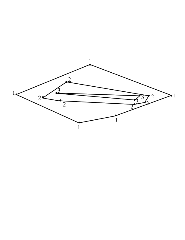
Figure 1: Convex layers.

Figure 2: Location layers.

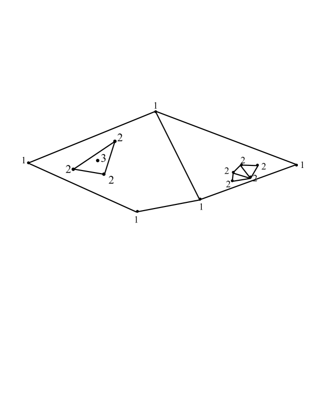
Figure 3: Delaunay layers.

3 Point set stratification

Given a set $S$ of $n$ points in the plane the convex layers can be constructed with Chazelle’s optimal $O(n\log n)$ algorithm [Cha85]. Convex layers form a sequence of nested convex polygons defining a partition of the plane into regions, which coincide with the levels, (Figures 1 and 4). Therefore layers and levels have linear complexity in the convex depth case and can be constructed in optimal $O(n\log n)$ time.

As for location depth, a worst case optimal algorithm for computing all $Lev_{i}^{S}(S)$, (where $n/3\leq i\leq n/2$) in $O(n^{2})$ time is obtained by using topological sweep in the dual arrangement of lines (see [Cla04], [MRR⁺03]). The boundaries of the levels, in this case, form a sequence of nested convex polygons. Points of $Lay_{i}^{S}(S)$ are in convex position and belong to the boundary of $Lev_{i}^{S}(S)$, but this boundary can also have other vertices not in $S$, (Figure 5). Some layers can be empty and different layers can cross each other (Figure 2). While the complexity of levels may reach $O(n^{2})$, the size of the layers is $O(n)$. The layers in the location depth case can be computed using the mentioned $O(n^{2})$ sweep algorithm yet, to our knowledge, it is an open problem to construct them in less time or to prove a quadratic lower bound for the problem.

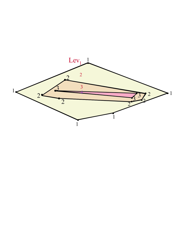
Figure 4: Convex levels.

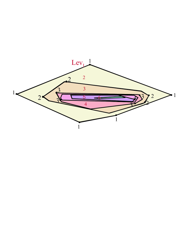
Figure 5: Location levels.

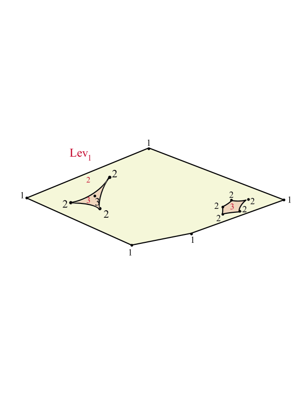
Figure 6: Delaunay levels.

Much less has been studied to Delaunay depth, which we explore sistematically in the rest of this section.

In the Delaunay depth case, all the layers $Lay_{i}^{D}(S)$, $i\leq n/3$, can easily be found by visiting $DT(S)$ in linear time once constructed, which requires $O(n\log n)$ time (Figure 3). Notice that one layer can have more than one connected component. Next, we study the Delaunay layers. First, we show some properties of Delaunay layers which allow us to obtain the levels easily and also to prove other results as that the $\bigcup Lev_{i}^{D}(S)$ are nested sets. Next, we will study the number of connected components that we can have in the $\bigcup Lay_{i}^{D}(S)$.

Proposition 3.1

Let $S$ be a set of Delaunay depth greater than one. The points of $S$, in the interior of any cycle $C_{i}$ of $Lay_{i}^{D}(S)$, have depth greater than $i$.

Proof. Let $p\in S$ be, which is in the interior of a cycle $C_{i}$ of $Lay_{i}^{D}(S)$. From the definition of Delaunay depth, we know that $p$ must have some adjacency of depth $d_{S}^{D}(p)-1$. The points adjacent to $p$ are points of $C_{i}$ or they are in the interior of $C_{i}$.

If we suppose the assertion of the proposition is false, $d_{S}^{D}(p)\leq i$. Then there exists a point $q$ adjacent to $p$, with $d_{S}^{D}(q)=d_{S}^{D}(p)-1$ and interior of $C_{i}$. Recursively it follows that there is at least a point of depth equal to $1$ in the interior of $C_{i}$, which is impossible. Then we conclude that all points of $S$ which are in the interior of $C_{i}$ have depth greater than $i$.

$\hfill\Box$

Lemma 3.1

Let $S$ be a set of Delaunay depth greater than one. Any cycle of $Lay_{i}^{D}(S)$ without chords, does not contain more than one connected components of $Lay_{i+1}^{D}(S)$ in its interior.

Proof. Let $C_{i}$ be a cycle of $Lay_{i}^{D}(S)$ formed by points without chords.

Suppose, contrary to our claim, that there are more than one connected component of $Lay_{i+1}^{D}(S)$ in the interior of $C_{i}$. By the above assumption, we first prove that there is a vertice $v_{i}\in C_{i}$ which is adjacent to some points of different connected components of $Lay_{i+1}^{D}(S)$ in the interior of $C_{i}$ (Figure 8). Let $v_{i}^{1},v_{i}^{2},\cdots,v_{i}^{n}$ be the points of $C_{i}$ sorted by adjacencies. We study the adjacencies of these points in the interior of $C_{i}$. Note that this adjacencies have depth equal to $i+1$ (we apply that their depth cannot differ more than one of $i$ and Proposition 3.1); furthermore, all the points of $Lay_{i+1}^{D}(S)$ in the interior of $C_{i}$ must have at least one adjacency in $C_{i}$.

We move along $C_{i}$ following the adjacencies: while the adjacencies are of the same connected component we are changing of point in $C_{i}$. We want to find different connected components in the adjacencies. There are two possibilities:

1. There is a point $v_{i}^{j}$ which is adjacent to some points of different connected components of $Lay_{i+1}^{D}(S)$ in the interior of $C_{i}$.

2. There are $v_{i}^{j}$ and $v_{i}^{j+1}$, for some $j$, whose adjacencies are in different components of $Lay_{i+1}^{D}(S)$ (Figure 7).

But in the second case, we can see that the point $v_{i}^{j}$ or $v_{i}^{j+1}$ must also have adjacencies in different components of $Lay_{i}(S)$ (is a point like in the first case). In order to prove that, we can consider the point which forms a triangle in the $DT(S)$ with $v_{i}^{j}$ and $v_{i}^{j+1}$. This point can only be of depth $i+1$; it cannot be $i$ because then $v_{i}^{j}v$ and $v_{i}^{j+1}v$ would be chords, contrary of the hypothesis of the proposition. Hence, $v\in Lay_{i+1}^{D}(S)$ but, $v$ cannot belong at the same time to the different connected components where $v_{i}^{j}$ and $v_{i}^{j+1}$ have adjacencies.

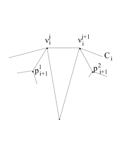
Figure 7: The points $v_{i}^{j}$ and $v_{i}^{j+1}$ of $C_{i}$ have adjacencies of different components of $Lay_{i+1}^{D}(S)$.

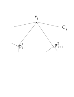
Figure 8: There is a point $v_{i}\in C_{i}$ adjacent to some points of different connected component of $Lay_{i+1}^{D}(S)$ in the interior of $C_{i}$.

We have proved that $v_{i}\in C_{i}$ exists with two adjacencies of different components of $Lay_{i+1}^{D}(S)$, we denote them by $p_{i+1}^{1},p_{i+1}^{2}$ like Figure 8. Then there is a path in the $DT(S)$ between $p_{i+1}^{1}$ and $p_{i+1}^{2}$ formed by a sequence of vertices of triangles which all they have $v_{i}$ as point in common. Note that this sequence only can be formed by points of depth $i+1$: there is no point with depth $i+2$ because this point is adjacent to $v_{i}$, of depth $i$ and also there is no a point of depth equal to $i$ because this point with $v_{i}$ would be a chord which contradicts the assumptions. The $Lay_{i+1}^{D}(S)$ is formed by the subgraph induced in the $DT(S)$ by the points with the same depth, so all the points adjacents to $v_{i}$, between $p_{i+1}^{1}$ and $p_{i+1}^{2}$, are in the same connected component, a contradiction.

Hence we conclude that any cycle of $Lay_{i}^{D}(S)$ without chords, does not contain more than one connected component of $Lay_{i+1}^{D}(S)$ in its interior.

$\hfill\Box$

Lemma 3.2

Let $S$ be a set of points in the plane. Let $p\in Lay_{i+2}^{D}(S)$ and let $C^{i}$ be a cycle of $Lay_{i}^{D}(S)$ that contains $p$ in its interior. Then there is a cycle of $Lay_{i+1}^{D}(S)$ containing $p$ in its interior.

Proof. Let $p_{i+2}\in$ D-$Lay_{i+2}(S)$ be a point in the interior of $C_{i}$. From Lema 3.1 we know that there is only one connected component of D-$Lay_{i+1}(S)$ in $C_{i}$.

When we consider a connected graph without cycles embedded in the plane, there is only a single infinite region, complementary to the graph. If the graph has some cycles, then we distinguish the bounded regions enclosed by the edges of the cycles. We will prove that the graph $G$ formed by the points with depth $i+1$ inside $C_{i}$ must be a graph with cycles. Its unbounded region contains $C_{i}$. Each point of the considered graph $G$ has depth $i+1$ and it is adjacent to one of the $C_{i}$. We consider the Delaunay triangles with at least one vertex in $C_{i}$. The point $p_{i+2}$ cannot be vertex of any of those triangles (the depths cannot differ in more than one unit). The union of those triangles does not contain $p_{i+2}$ because the Delaunay triangles do not contain points of $S$ in their interior. Only if $G$ has some cycles, there can be other points placed in the bounded regions delimited by them. Therefore, if there exists a point of D-$Lay_{i+2}(S)$ in the interior of $C_{i}$, then there exists too a cycle of D-$Lay_{i+1}(S)$ containing such point in its interior.

$\hfill\Box$

Proposition 3.2

Let $S$ be a set of points in the plane. If the Delaunay depth of a point $p$ with respect to $\,S\,$ is $j+1$, there is a cycle of $Lay_{j}^{D}(S)$ containing $p$ in its interior.

Proof. Every point $p$ whose depth with respect to $\,S\,$ equals $2$, is contained in the interior of $Lay_{1}^{D}(S)=CH(S)$.

If the depth of $p$ is $3$, there exists a cycle of $Lay_{2}^{D}(S)$ containing $p$ in its interior. In order to prove that, we apply Lemma 3.2 to a cycle of points of depth $1$ that contains $p$ (this cycle exists because $Lay_{1}^{D}(S)=CH(S)$).

If the depth of $p$ is $4$, there is a point of $Lay_{3}^{D}(S)$ adjacent to $p$. We apply Lemma 3.2 to this point of depth $3$. Then there is a cycle of $Lay_{2}^{D}(S)$ that contains this point of depth $3$, and must contain its adjacencies, like $p$. We apply lemma 3.2 to this last cycle and there is a cycle of $Lay_{3}^{D}(S)$ that contains $p$.

Recursively we prove the proposition for $p$ of depth $j+1$ $\forall j,j\leq f-1$ ($f$ being the depth of $S$).

$\hfill\Box$

As a consequence of Proposition 3.2, the number of levels for Delaunay depth is equal to the number of layers or to the number of layers plus one.

Proposition 3.3

Let $S$ be a set of $n$ points. The maximum number of connected components of the $\bigcup Lay_{i}^{D}(S)$ is decreasing on the depth of $S$. This maximum is $\displaystyle{\lfloor(n-m+2)/2\rfloor}$, where $m$ is the depth of $S$, which is tight.

Proof. We want to see that $c$, the number of connected components of $\bigcup Lay_{i}^{D}(S)$, is bounded by $(n-m+2)/2$ or, equivalently, $n\geq 2c+m-2$.

If all the related connected components have a minimum of $2$ points, then $n\geq 2c$. If there are isolated points in $Lay_{i+1}^{D}(S)$, each one of them is contained in a cycle without chords (Proposition 3.2). We associate each isolated point with a point of the corresponding cycle in this way: two isolated points cannot be associated to the same point. This is possible because the maximum number of the isolated points of $Lay_{i+1}^{D}(S)$, contained in a connected component of $Lay_{i}^{D}(S)$, is at most the number of chords plus one (Lemma 3.1). Moreover, the number of chords in a connected component of $n_{i}$ points is at most $n_{i}-3$ so there are no points of depth $i$ in the interior of a cycle of $Lay_{i}^{D}(S)$ (Proposition 3.1).

Then, there are at least two points in each component that are not associated to any of the possible isolated points. Thus we can assure $n\geq 2c$.

In general, if the depth of $S$ is $m$, there exist at least $m-1$ nested cycles, without chords, of which $m-2$ don’t contain any component of a single point. The connected component that contains one of the previous cycles have, at most, $n_{i}-3$ isolated points. Therefore, there are at least $m-2$ connected components with three points or more. Then $n\geq 2c+m-2$.

The next example proves that the previous upper bound is tight.

First we describe the example for $m=2$. Let $n=2k+2$ be the number of points that we have. We distinguish two chains in the $CH(S)$: in one of them (for example the lower chain) we put $k+1$ of the points of $S$ and in the other (the upper chain) we put only one point. We can place the points in this way: for every pair of points formed with the upper chain point and any lower chain point, there must be an empty circle that circumscribes them. Finally, we put each one of the other $k$ points of $S$ between two of the previous circles like in Figure 9. These $k$ points are each one of them one connected component of $Lay_{2}^{D}(S)$, so the $\bigcup Lay_{i}^{D}(S)$ has $k+1=\lfloor n/2\rfloor$ connected components.

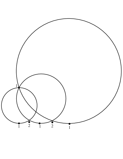
Figure 9: This is a example in which $n=2k+2$ points. The $\bigcup Lay_{i}^{D}(S)$ has $k+1$ connected components.

Let $m$ be greater than $2$. First we put $3(m-1)$ points in a sequence of nested triangles and one more point in the innest one. The rest of the points of $S$, at most $n-3m+2$, are distributed in pairs between the $m$ layers. We place each pair of the points in contiguous layers so one of them breaks a cycle in two and the other one is an isolated point in the new cycle. In figure 10, the $n-3m+2$ points have been placed in the layers $Lay_{1}^{D}(S)$ and $Lay_{2}^{D}(S)$.

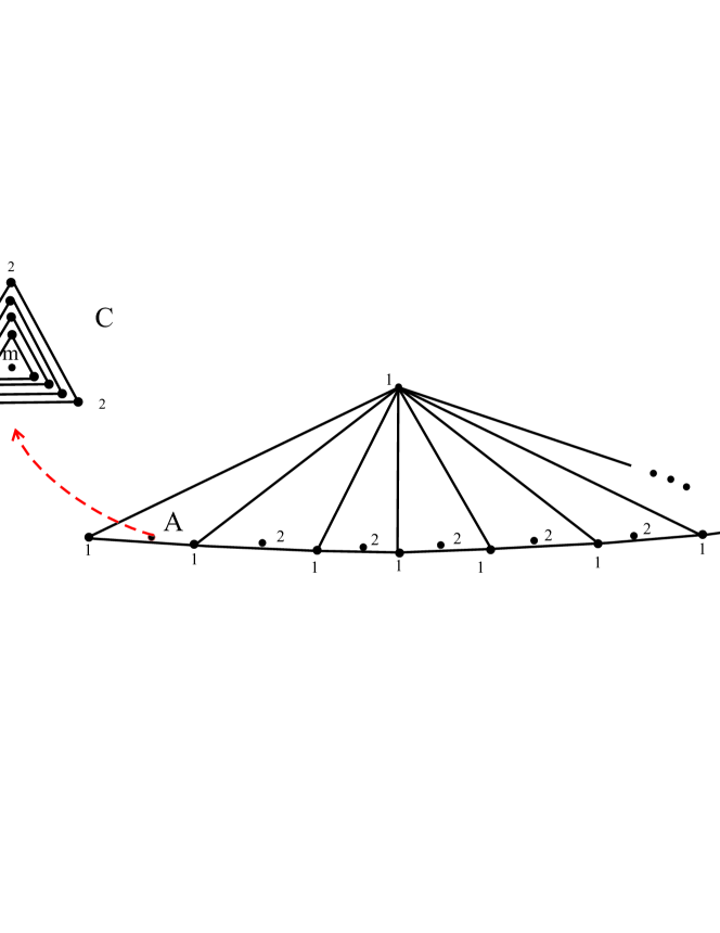
Figure 10: Point $A$ is replaced by configuration $C$. The set of points $S$ has depth equal to $m$. The $\bigcup Lay_{i}^{D}(S)$ has $\lfloor(n-m+2)/2\rfloor$ connected components.

$\hfill\Box$

Delaunay layers are not necessarily polygons, however they form a structure based in nested cycles of points of the same depth.

The depth of a point relative to a set $S$ depends on the Delaunay circles (i.e., circumcircles of Delaunay triangles) that contain the point, therefore the arrangement of Delaunay circles contains all the information about Delaunay levels, (Figure 6). As the arrangement has size $O(n^{2})$ and can be constructed in $O(n^{2}\log n)$ time one can obtain the Delaunay levels within this time. Nevertheless, in the following theorem we prove that in order to obtain all $Lev_{i}^{D}(S)$ it is not necessary to construct the whole arrangement of circles.

Observation 3.3

Let $C$ be a circle having exactly two points $u$ and $v$ of $S$ on its boundary and containing no points of $S$ in its interior. Then any circle crossing the two arcs determined by $u$ and $v$ in the boundary of $C$ contains some interior point from $S$.

Theorem 3.4

Let $S$ be a set of points in the plane and let be $f$ its Delaunay depth. The union $\bigcup_{j\geq k}Lev_{j}^{D}(S)$, $k=1,\cdots,f$ forms a sequence of sets nested by inclusion. The boundaries between $Lev_{j}^{D}(S)$ and $Lev_{j+1}^{D}(S)$, for $2\leq j\leq f$, are curves composed by arcs of the Delaunay circles determined by two points $u,v$ of $Lay_{j}^{D}(S)$ and one point $w$ of $Lay_{j-1}^{D}(S)$.

Proof. We proceed to determine the boundary between the consecutive levels of $S$, $Lev_{j}^{D}(S)=\{x\in\mathbb{R}^{2}/d(x,S)=j\}$, and $Lev_{j+1}^{D}(S)$, for $2\leq j\leq f$. Every point $q$ of depth equal to $j$, relative to a set $S$, has at least one element $p\in S$ which is adjacent in $DT(S\cup\{q\})$ and has depth $j-1$ (in both $DT(S)$ and $DT(S\cup\{q\})$), and there must be an empty circle through $p$ and $q$ and no point of $S$ with depth smaller than $j-1$. Hence we can describe the $Lev_{j}^{D}(S)$ as the union of all Delaunay circles that circumscribe a point of depth $j-1$ (that we denote by $\bigcup C_{j-1,-,-}$), minus the union of all Delaunay circles that circumscribe a point of depth smaller than $j-1$ (that we denote by $\bigcup C_{<j-1,-,-}$); this is

$$Lev_{j}^{D}(S)=\bigcup C_{j-1,-,-}\setminus\bigcup C_{<j-1,-,-}.$$

Applying Proposition 3.2, which proves that for every point of depth equal to $j$ there is a cycle of $Lay_{j-1}^{D}(S)$ that contains it in its interior, we see that $Lev_{j}^{D}(S)$ is contained in the interior of the cycles of $Lay_{j-1}^{D}(S)$. Furthermore we also get the following properties: (a) If some layer has no cycles then there are no points for this level or the next ones; (b) the sets $\bigcup_{j\geq k}Lev_{j}^{D}(S),\,k=1,\cdots,f$ form a sequence of nested sets.

We find circles $C_{j,j,j-1}\in\bigcup C_{<j,-,-}$ intersecting the cycles of $Lay_{j}^{D}(S)$. The circles $C_{j,j,j-1}$ pass through pairs of points which are the endpoints of every non-chord edge of a cycle $\gamma$ in $Lay_{j}^{D}(S)$ (see the cycle of $Lay_{3}^{D}(S)$ enclosing the dark region to the left of Figure 11).

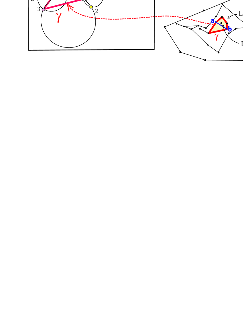
Figure 11: The Delaunay circles $C_{3,3,2}$ defined by two points of $Lay_{3}^{D}(S)$ and one point of $Lay_{2}^{D}(S)$, determine the boundary between $Lev_{3}^{D}(S)$ and $Lev_{4}^{D}(S)$, which consists of the inner boundary of the union of $C_{3,3,2}$. Notice that chord $ab$ has been “discarded”, as unuseful for obtaing the level.

These pairs of points divide the circle $C_{j,j,j-1}$ into two arcs: one exterior to the cycle $\gamma$, one interior. There may be other circles of $\bigcup C_{<j,-,-}$ that also cross the circle $C_{j,j,j-1}$, yet any circle of $\bigcup C_{<j,-,-}$ has in the boundary one point exterior to the cycle $\gamma$ and, applying Observation 3.3, it cannot cross both arcs of a circle $C_{j,j,j-1}$.

Therefore the boundary between $Lev_{j}^{D}(S)$ and $Lev_{j+1}^{D}(S)$ is only determined by the arcs of the circles $C_{j,j,j-1}$ (see Figure 12 for an illustration).

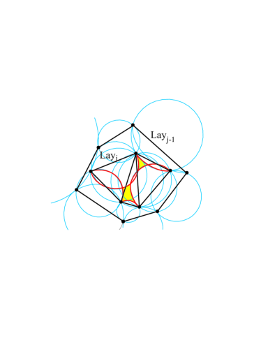
Figure 12: The shaded region is $Lev_{j+1}^{D}(S)$.

$\hfill\Box$

Theorem 3.4 proves that the overall size of the Delaunay levels is $O(n)$ and justifies the steps of the following algorithm.

Algorithm 3.1

Computation of Delaunay depth contours of $S$, Delaunay levels.

Input: Set of points $S$.

Output: Delaunay depth contours of $S$.

1. Compute $DT(S)$.

2. Compute the Delaunay depths for all points in $S$.

3. Compute the boundaries of the levels as follows: $Lev_{1}^{D}(S)$ is the convex hull of $S$; for every $j\geq 2$, construct the inner boundary of the union of Delaunay circles $C_{j,j,j-1}$ defined by two points $u,v$ of $Lay_{j}^{D}(S)$ and one point $w$ of $Lay_{j-1}^{D}(S)$ (Figure 12).

$DT(S)$ can be computed in $O(n\log n)$ time and Step $2$ takes $O(n)$ additional time. Every boundary in Step $3$ can be computed in $O(t\log^{2}t)$ time, where $t$ is the number of Delaunay circles $C_{j,j,j-1}$ considered in the currently computed layer, by using the algorithm described in [AS00] (pg. 97). Taking into account that the total number of Delaunay circles is $O(n)$, Step $3$ takes $O(n\log^{2}n)$ global time, which is also the overall time for the algorithm. Notice that the expected time for Step 3 is $O(n\log n)$ [AS00], and therefore, the expected running time for the entire algorithm is $O(n\log n)$.

The algorithm 3.1 compute all levels of $S$ in $O(n\log^{2}n)$ time, therefore it also yields the Delaunay median in this time. In Figure 13 we can see an illustration where the inner level, $Lev_{6}^{D}(S)$, has two connected components: the centroids of each one of these regions are the Delaunay median of $S$.

As a consequence of the preceding paragraphs we can state the following theorem.

Theorem 3.5

The Delaunay levels of a set of $n$ points in the plane can ce constructed within $O(n\log^{2}n)$ time.

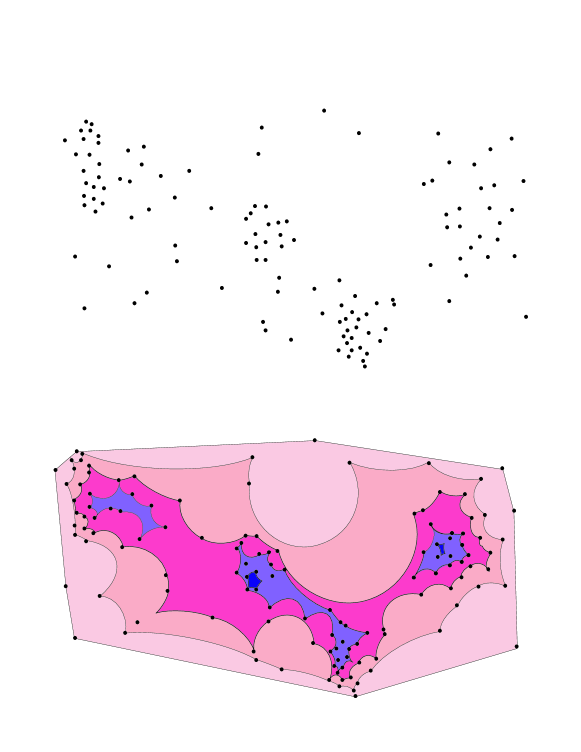
Figure 13: Top: A point set $S$. Bottom: Levels of $S$. The boundaries of the levels are the Delaunay depth contours.

4 Computing Delaunay depth

The depth of a point $p$ with respect to a data set $S=\{s_{1},\cdots,s_{n}\}$ in the plane is defined as the depth of $p$ in $S\cup\{p\}$, and its computation is a problem which has deserved much attention. When $S$ and $p$ are the entry data, the Tukey depth of $p$, its simplicial depth and its Oja depth can be computed in $O(n\log n)$ [RR96]. In [ACG⁺02] it was proved that this value is also a tight bound for the first two cases and recently it has been proved an identical result for the Oja depth [AMcL04] .

The convex depth of $p$ can be easily computed in $O(n\log n)$ time, since it suffices to find the layers of $S\cup\{p\}$, and it is easy to see that this value is tight. The Delaunay depth can also be found in $O(n\log n)$, since it suffices to build $DT(S\cup\{p\})$ and then find the depth of $p$ in additional $O(n)$ time. We will next show that this is tight.

We will reduce the problem of uniqueness of numbers to the problem of finding the Delaunay depth. It is known that the problem of deciding if, given $n$ real numbers, all of them are distinct, has complexity $\Omega(n\log n)$ when the model of computation is the algebraic decision tree [DL76] and [BO83]. We will see that if certain computations are made in $O(n)$ and then the Delaunay depth of an adequate point is found, we can decide the uniqueness of $n$ given real numbers. This implies that the computation of the Delaunay depth requires $\Omega(n\log n)$ time.

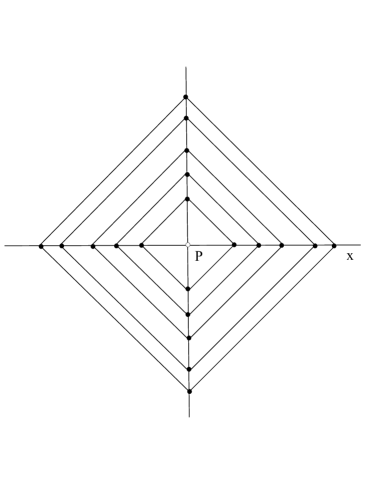
Figure 14: Set of points $A$ and its Delaunay layers.

Let us consider a set $A=\{x_{1},\cdots,x_{n}\}$ of real numbers; without loss of generality we can assume that they are all positive. For each value $x_{i}\in A$, we construct the points $(x_{i},0),(-x_{i},0),(0,x_{i})$ and $(0,-x_{i})$. We denote by $S$ the union of these points and let $p=(0,0)$ be the origin. The Delaunay triangulation $DT(S\cup\{p\})$ is as shown in Figure 14, from which we have omitted the diagonals of the trapezium (any of the two diagonals in a trapezium gives a Delaunay triangulation and the depths of the points remain unaltered by the choice). The presence of the edges of slopes $\pm 1$ is immediate: for example, $(x_{i},0)$ is adjacent to $(0,x_{i})$ since the circle of center $(x_{i},x_{i})$ and radius $x_{i}$ covers only these two points of $S\cup\{p\}$.

Evidently, the depth of $p$ in $S\cup\{p\}$ equals $n+1$ if, and only if, all the elements of $A$ are distinct. This completes the proof. It has thus been established the following result:

Theorem 4.1

The depth of a point $p$ with respect to a data set $S=\{s_{1},\cdots,s_{n}\}$ can be found in $O(n\log n)$ time, and this value is optimal.

If we admit an additional preprocess to the given point set, we have different alternatives for computing the level of a new point. For example the preprocessing might consist of computing the Delaunay triangulation, or even the arrangement of the Delaunay circles; nevertheless the most natural approach is to compute the Delaunay levels in a first step, which requires $O(n\log^{2}n)$ time; as this gives a plane subdivision of size $O(n)$, standard point-location methods can then be used. In particular, the approach in [ST86] can be easily adapted and allows $O(\log n)$ query time.

It is also natural to consider how strong the change in the Delaunay depths of a point set can be after the insertion of a new point. This is the issue we study next.

Proposition 4.1

Let $S$ be a set of $n$ points of depth equal to $f$. The insertion of one point in $S$ can change the depth of another point in at most $\lfloor n/3\rfloor-2$ units and the depth of the set can vary by $\displaystyle{\lfloor n/3\rfloor-3}$. These bounds are tight.

Proof. One point can vary its depth when its set of neighbors varies (for instance when $p$ is a new neighbor) or some of its neighbors changes its depth. The insertion of one point in $S$ can produce at most a change of depth equal to $f-2$ units, if and only if some of the deepest points is a neighbor of the least deep one.

Let us see now an example of a point set $S$ with depth $n/3$, in which the insertion of a suitable point modifies the depth of a certain point from $f=n/3$ to $2$. Let us consider two triangles homothetic from their common circumcenter such that the circumcircle $C$ of the inner triangle $T_{int}$crosses twice each edge of the outer triangle $T_{ext}$(see Figure 15). Then $S$ is defined by taking the six vertices of the triangles and placing evenly points in the segments $s_{1}$ $s_{2}$ and $s_{3}$) that join corresponding vertices of both triangles. Notice that the interior of the disk bounded by $C$ is empty of points of $S$ and that part of it is outside $CH(S)$. The Delaunay layers of $S$ are triangles and the depth of $S$ is $n/3$; layers and levels are shown in Figure 16 (top).

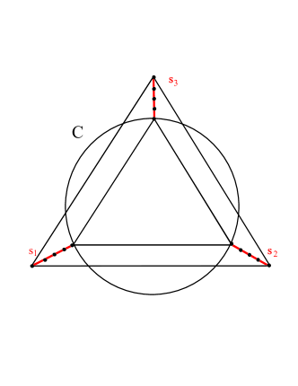
Figure 15: The points of $S$ lie on the segments $s1$, $s_{2}$ and $s_{3}$.

We insert now a point $p$ (refer to Figure 16) which is exterior to $CH(S)$ and interior to the disk bounded by $C$. In this way, $p$ is adjacent to the three vertices of $T_{int}$ and to all points placed on the two closest segments $s_{i}$, let them be, for example, $s_{1}$ and $s_{2}$. Hence $p$ is adjacent to points of depth $n/3$ in $S$ (the vertices of $T_{int}$) and to points of depth $1$ (the vertices of $T_{ext}$).

Let us compute the depths in the $S\cup\{p\}$. The point $p$ has depth $1$ (it is exterior to $CH(S)$) and any of its neighbors that is not in that hull has now depth $2$. Therefore, at least one point of depth equal to $n/3$ in $S$, has depth $2$ in $S\cup\{p\}$, a change as claimed.

The points of depth $1$ and $2$ in $S$ have still the same depth in $S\cup\{p\}$. The edges of $DT(S\cup\{p\})$ with an endpoint in $s_{3}$ are the same as in $DT(S)$; only edges between $s_{1}$ and $s_{2}$ have changed. As a consequence, the point of $Lay_{2}^{D}(S)$ from $s_{3}$ and the neighbors of $p$ in $Lay_{2}^{D}(S\cup\{p\})$ determine a cycle of $Lay_{2}^{D}(S\cup\{p\})$ (Figure 16, bottom, left). The other points that remain on $s_{3}$ are of depth $3$. Therefore, after the insertion of $p$, de depth of $S$ changes from $n/3$ to $3$.

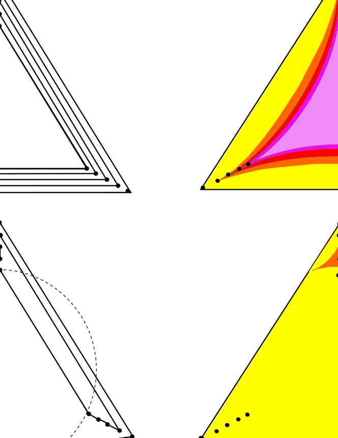
Figure 16: Delaunay layers and levels of the sets of points $S$ (at the top) and $S\cup\{p\}$ (at the bottom).

$\hfill\Box$

5 Conclusion

In this work we have studied the Delaunay depth function, the stratification that this depth induces in the point set (layers) and in the whole plane (levels), and developed algorithms for computing the Delaunay depth contours and the depth of any query point set with respect to the given point set. The stratification suggests that Delaunay depth may be more suitable than others for cluster detection and visualization.

As for open problems, let us mention that we don’t know whether a Delaunay median, i.e., a point of maximal depth, can be computed directly, escaping depth computation for the whole point set.

References

- [ACG+02] G. Aloupis, C. Cortés, F. Gómez, M. Soss, G. Toussaint. Lower bounds for computing statistical depth. Computational Statistics & Data Analysis 40:223–229, 2002.
- [AMcL04] G. Aloupis, E. McLeish. A Lower Bound for Computing Oja Depth. To appear in Information Processing Letters, accepted May 2005.
- [AS00] P. Agarwal, M. Sharir, Arrangements and its applications, in Handbook of Comput. Geom., J.R. Sack and J. Urrutia eds., North-Holland 2000.
- [Ba76] V. Barnett. The ordering of multivariate data (with discussion). Journal of the Royal Statistical Society Series A 139, 318–352, 1976.
- [BH99] Z.D. Bai, X. He. Asymptotic distributions of the maximal depth estimators for regression and multivariate location. Ann. Statist. 27:1616–1637, 1999.
- [BO83] M. Ben-Or. Lower bounds for algebraic computaton trees. Proc. 15th. Ann. ACM Sympos. Theory Comput., 80–86, 1983.
- [Cha85] B. Chazelle. On the Convex Layers of a Planar Set, IEEE Transactions on Information Theory IT-31:4 509–517, 1985.
- [Cla04] M. Claverol, Geometric Problems on Computational Morphology. Ph. D Thesis, UPC, Barcelona, 2004.
- [CSY87] R. Cole, M. Sharir, C.K. Yap. On K-hulls and related problems, SIAM Journal of Computing 16:61–77, 1987.
- [DL76] D. Dobkin, R. Lipton. Multidimensional searching problems. SIAM J. Comput., 5(2):181–186, 1976.
- [Epps97] D. Eppstein. Fast hierarchical clustering and other applications of dynamic closest pairs. Proc. 9th Annu. ACM-SIAM Sympos. Discrete Algorithms 131–138, New Orleans, 1997.
- [Gre81] P.J. Green. Peeling Bivariate Data. In: Interpreting multivariate data. John Wiley and Sons Ltd., 163–198, 1981.
- [Hu72] P.J. Hubert. Robust statistics: a review. Ann. Math. Statistics 43:3 1041–1067, 1972.
- [Ki83] D.G. Kirkpatrick. Optimal search in planar subdivisions. SIAM J. of Computing, 12:28–35, 1983.
- [LS00] S. Langerman, W. Steiger. An optimal algorithm for hyperplane depth in the plane. In Proc. 11th Ann. ACM-SIAM Sympos. Discrete Algorithms, 54–59, San Francisco, 2000.
- [Liu90] R.Y. Liu. On a notion of data depth based on random simplices. Ann. Statist., 18:405–414, 1990.
- [LPS99] R.Y. Liu, J. Paralelius, K. Singh. Multivariate analysis by data depth: descriptive statistics, graphics and inference. Ann. Statist., 27:783–840, 1999.
- [MRR+03] H.K. Miller, S. Ramaswami, P. Rousseeuw, T. Sellares, D. Souvaine, I. Streinu, A. Struyf. Efficient computation of location depth contours by methods of Computational Geometry. Statistics and Computing, 2003.
- [NTM01] A. Nanopoulos, Y. Theodoridis, Y. Manolopoulos. : Clustering based on Closest Pairs. Proc. of the 27th VLDB Conference., Roma, 2001.
- [Oja83] H. Oja. Descriptive statistics for multivariate distributions. Statist. Probab. Lett., 1:327–332, 1983.
- [OBS92] A. Okabe, B. Boots, K. Sugihara. Spatial Tessellations: Concepts and Applications of Voronoi Diagrams. John Wiley and Sons Ltd. Chichester, 362–363, 1992.
- [RH99] P.J. Rousseeuw, M. Hubert. Regression depth. J. Amer. Statist. Assoc., 94:388–402, 1999.
- [RR96] P.J. Rousseeuw, I. Ruts. Algorithm AS 307: bivariate location depth. J. Roy. Statist. Soc. Ser. C, 45:516–526, 1996.
- [RS04] P.J. Rousseeuw, A. Struyf. Computation of robust statistics: depth, median, and related measures, in Handbook of Discrete and Comput. Geom., J.E. Goodman and J. O’Rourke eds., Discrete Mathematics and Its Applications, 2004.
- [ST86] N. Sarnak, R. E. Tarjan. Planar point location using persistent search trees. Communications of the ACM, 29(7):669–679, 1986.
- [Sib81] R. Sibson. A brief description of natural neighbour interpolation, in: Interpolating multivariate data. John Wiley y Sons Ltd., 21–36, 1981.
- [Sma90] C.G. Small. A survey of multidimensional medians. Internat. Statistical Review, 58:263–277, 1990.
- [SHR97] A. Struyf, M. Hubert, P.J. Rousseeuw. Integratint robust clustering techniques in S-PLUS. Comput Statist. Data Anal., 26:17–37, 1997.
- [Tu75] J.W. Tukey, Mathematics and the picturing of data. Proc. of the Intern. Congress of Mathematicians, 2:523–531, 1975.
- [ZS00] Y. Zuo, R. Serfling. General notions of statistical depth functions, Ann. Statist., 28:461–482, 2000.