Asymptotic Capacity Results for Non-Stationary Time-Variant Channels Using Subspace Projections

Abstract

In this paper we deal with a single-antenna discrete-time flat-fading channel. The fading process is assumed to be stationary for the duration of a single data block. From block to block the fading process is allowed to be non-stationary. The number of scatterers bounds the rank of the channels covariance matrix. The signal-to-noise ratio (SNR), the user velocity, and the data block-length define the usable rank of the time-variant channel subspace. The usable channel subspace grows with the SNR. This growth in dimensionality must be taken into account for asymptotic capacity results in the high-SNR regime. Using results from the theory of time-concentrated and band-limited sequences we are able to define an SNR threshold below which the capacity grows logarithmically. Above this threshold the capacity grows double-logarithmically.

I Introduction

In this paper we deal with a single-antenna discrete-time flat fading channel. The fading process is assumed to be stationary and Gaussian for the duration of a single data block of length $M$. From block to block the fading process is allowed to be non-stationary, i.e., we assume the fading to be independent across blocks. We analyze the validity of subspace based channel models for obtaining high signal-to-noise ratio (SNR) capacity results.

In wireless communication system the time-variation of the communication channel is caused by Doppler effects due to user movement and multipath propagation. The Doppler bandwidth of the channels time-variation is defined by the velocity of the user. The symbol rate is typically much higher than the maximum Doppler bandwidth.

In [1] the capacity of a non-coherent block-stationary fading model is analyzed and the pre-log (i.e., the ratio of capacity to $\log\mathrm{SNR}$ in the limit when the $\mathrm{SNR}$ tends to infinity $\lim_{\mathrm{SNR}\rightarrow\infty}\frac{C(\mathrm{SNR})}{\log\mathrm{SNR}}$ ) is derived. The pre-log depends critically on the rank of the covariance matrix of one fading block. In order to estimate this rank for realistic scenarios Liang and Veeravalli use in [1] a subspace projection on Fourier basis functions [2]. Their derivation, however, lacks several important points:

• A projection of the time-variant channel $h[\cdot]$ on a subspace makes only sense in a context where $h[\cdot]$ needs to be estimated, e.g., from the observed channel output symbols. This means that the estimation becomes dependent on the $\mathrm{SNR}$.

• Any estimation problem is based on a criterion that allows to specify the quality of a particular estimate. In [1] no such criterion is given. We propose to use a mean square error (MSE) criterion.

• Once the problem of defining a subspace is understood as estimation problem with a given quality-criterion, it becomes obvious that the choice of the basis functions strongly influences the estimation error. In particular, the Fourier basis expansion, i.e., a truncated discrete Fourier transform (DFT), has the following major drawback in describing a time-variant channel: the rectangular window associated with the DFT introduces spectral leakage [3, Sec. 5.4], i.e., the energy from low frequency Fourier coefficients leaks to the full frequency range. Furthermore, the truncation causes an effect similar to the Gibbs phenomenon [3, Sec. 2.4.2]. This leads to significant phase and amplitude errors at the beginning and at the end of a data block, and hence to a deteriorated MSE.

• The choice of the dimension of the subspace has to be made in the context of the estimation problem. Hence, the optimum dimension will depend on the $\mathrm{SNR}$ by the trade-off between the square bias and the variance [4, 5].

We suggest two subspace projections that give a significantly better MSE than the Fourier basis expansion of [1]:

• The Slepian basis expansion, as introduced in [4] based on concepts from the theory of time-concentrated and band-limited sequences [6], offers a square-bias reduction of more than one magnitude compared to the Fourier basis expansion [4].

• The Karhunen-Loève expansion provides the optimum basis functions in terms of a minimum MSE when the second order statistics are known.

Contribution:

• We adapt the results from [1] taking into account the SNR-dependent subspace dimension.

• We define a SNR threshold below which the capacity grows logarithmically. Above this threshold the capacity grows double-logarithmically. This result allows to bridge the gap between the results from [1] and [7].

The rest of the paper is organized as follows:

The notation is presented in Section II and the signal model for flat-fading time-variant channels is introduced in Section III. We provide the time-variant channel description based on physical wave propagation principles in Section IV. Subspace based channel models are reviewed in Section V building the foundation for the capacity results in Section VI which build on [1]. In Section VII numerical results for the begin of the double-logarithmic capacity region are presented. We draw conclusions in Section VIII.

II Notation

$\textstyle a$	column vector with elements $a[i]$
$\textstyle A$	matrix with elements $[{\mathchoice{\mbox{\boldmath$\displaystyle A$}}{\mbox{\boldmath$\textstyle A$}}{\mbox{\boldmath$\scriptstyle A$}}{\mbox{\boldmath$\scriptscriptstyle A$}}}]_{i,\ell}$
${\mathchoice{\mbox{\boldmath$\displaystyle A$}}{\mbox{\boldmath$\textstyle A$}}{\mbox{\boldmath$\scriptstyle A$}}{\mbox{\boldmath$\scriptscriptstyle A$}}}^{\mathrm{T}}$, ${\mathchoice{\mbox{\boldmath$\displaystyle A$}}{\mbox{\boldmath$\textstyle A$}}{\mbox{\boldmath$\scriptstyle A$}}{\mbox{\boldmath$\scriptscriptstyle A$}}}^{\mathrm{H}}$	transpose, conjugate transpose of $\textstyle A$
$\mathrm{diag}({\mathchoice{\mbox{\boldmath$\displaystyle a$}}{\mbox{\boldmath$\textstyle a$}}{\mbox{\boldmath$\scriptstyle a$}}{\mbox{\boldmath$\scriptscriptstyle a$}}})$	diagonal matrix with entries $a[i]$
${\mathchoice{\mbox{\boldmath$\displaystyle I$}}{\mbox{\boldmath$\textstyle I$}}{\mbox{\boldmath$\scriptstyle I$}}{\mbox{\boldmath$\scriptscriptstyle I$}}}_{Q}$	$Q\times Q$ identity matrix
$a^{*}$, $\left|a\right|$	complex conjugate, absolute value of $a$
$\lfloor a\rfloor$	largest integer, lower or equal than $a\in\mathbb{R}$
$\lceil a\rceil$	smallest integer, greater or equal than $a\in\mathbb{R}$
$\left\|{\mathchoice{\mbox{\boldmath$\displaystyle a$}}{\mbox{\boldmath$\textstyle a$}}{\mbox{\boldmath$\scriptstyle a$}}{\mbox{\boldmath$\scriptscriptstyle a$}}}\right\|$	$\ell_{2}$-norm of vector $\textstyle a$

III Signal Model for Flat-Fading Time-Variant Channels

We consider the transmission of a symbol sequence $d[m]$ with symbol rate $R_{\mathrm{S}}=1/T_{\mathrm{S}}$ over a time-variant flat-fading channel. The symbol duration is much longer than the delay spread of the channel $T_{\mathrm{S}}\gg T_{\mathrm{D}}.$ Discrete time is denoted by $m$. The channel in equivalent baseband notation $h(t,\tau)$ incorporates the transmit filter, the physical channel and the matched receive filter.

Hence, we consider a discrete time model where the received sequences $y[m]$ is given by the multiplication of the symbol sequence $d[m]$ and the sampled time-variant channel $h[m]\triangleq h(mT_{\mathrm{S}},0)$ plus additional circular symmetric complex white Gaussian noise $z[m]$

$$y[m]=\sqrt{\mathrm{SNR}}h[m]d[m]+z[m]\,,\qquad m\in\{0,\ldots,M-1\}\,.$$ (1)

The transmission is block oriented with block length $M$. The time-variant channel is assumed to be independent from block to block. We normalize the system so that the channel inputs $d[m]$ have power constraint $|d[m]|^{2}=1$, the channel coefficients $h[m]$ are circular symmetric complex Gaussian distributed with zero mean, $h[m]\sim\mathcal{CN}(0,1)$, and $z[m]$ is a sequence of independent and identically distributed (i.i.d.) $\mathcal{CN}(0,1)$ random variables. The term $\mathrm{SNR}$ presents the signal-to-noise ratio.

IV Physical Wave Propagation Channel Model

We model the fading process using physical wave propagation principles [8]. The impinging wave fronts at the receive antenna are caused by $P$ scatterers. The individual paths sum up as

$$h[m]=\sum_{p=0}^{P-1}a_{p}\mathrm{e}^{\mathrm{j}2\pi f_{p}T_{\mathrm{S}}m}=\sum_{p=0}^{P-1}a_{p}\mathrm{e}^{\mathrm{j}2\pi\nu_{p}m}\,.$$ (2)

Here $f_{p}\in\mathbb{R}$ is the Doppler shift of path $p$. For easier notation we define the normalized Doppler frequency as $\nu_{p}=f_{p}T_{\mathrm{S}}$. The attenuation and phase shift of path $p$ is denoted by $a_{p}\in\mathbb{C}$. The Doppler shift of each individual path $p$ depends on the angle of arrival $\alpha_{p}$ in respect to the movement direction, the users velocity $v$, and the carrier frequency $f_{\mathrm{C}}$,

$$\nu_{p}=\frac{vf_{\mathrm{C}}}{c_{0}}T_{\mathrm{S}}\cos\alpha_{p}\,.$$ (3)

The speed of light is denoted by $c_{0}$. The one sided normalized Doppler bandwidth is given by

$$\nu_{\mathrm{D}}=\frac{vf_{\mathrm{C}}}{c_{0}}T_{\mathrm{S}}\geq|\nu_{p}|\,.$$ (4)

It is assumed that $a_{p}$ and $\nu_{p}$ for $p\in\{0,\ldots,P-1\}$ are independent of each other and that both parameter sets are i.i.d..

We assume a time-variant block fading channel model. In this model the path parameters $a_{p}$ and $\nu_{p}$ are assumed to be constant for the duration of a single data block with length $M$. Their realization for the next data block is assumed to be independent. The fading process for the duration of a single data block is stationary, however from block to block the fading is non-stationary. This assumption is validated by measurement results from [9, 10].

We define the covariance matrix

$${\mathchoice{\mbox{\boldmath$\displaystyle\Sigma$}}{\mbox{\boldmath$\textstyle\Sigma$}}{\mbox{\boldmath$\scriptstyle\Sigma$}}{\mbox{\boldmath$\scriptscriptstyle\Sigma$}}}_{h}=\mathop{\mathbb{E}}\{{\mathchoice{\mbox{\boldmath$\displaystyle h$}}{\mbox{\boldmath$\textstyle h$}}{\mbox{\boldmath$\scriptstyle h$}}{\mbox{\boldmath$\scriptscriptstyle h$}}}{\mathchoice{\mbox{\boldmath$\displaystyle h$}}{\mbox{\boldmath$\textstyle h$}}{\mbox{\boldmath$\scriptstyle h$}}{\mbox{\boldmath$\scriptscriptstyle h$}}}^{\mathrm{H}}\}$$ (5)

where the channel coefficients for a single block with length $M$ are collected in the vector

$${\mathchoice{\mbox{\boldmath$\displaystyle h$}}{\mbox{\boldmath$\textstyle h$}}{\mbox{\boldmath$\scriptstyle h$}}{\mbox{\boldmath$\scriptscriptstyle h$}}}=[h[0],h[1],\ldots,h[M-1]]^{\mathrm{T}}\,.$$ (6)

Referring to (2) it is clear that the rank of ${\mathchoice{\mbox{\boldmath$\displaystyle\Sigma$}}{\mbox{\boldmath$\textstyle\Sigma$}}{\mbox{\boldmath$\scriptstyle\Sigma$}}{\mbox{\boldmath$\scriptscriptstyle\Sigma$}}}_{h}$ is given by

$$\mathrm{rank}({\mathchoice{\mbox{\boldmath$\displaystyle\Sigma$}}{\mbox{\boldmath$\textstyle\Sigma$}}{\mbox{\boldmath$\scriptstyle\Sigma$}}{\mbox{\boldmath$\scriptscriptstyle\Sigma$}}}_{h})=\min(P,M)=Q$$ (7)

for $v>0$.

V Subspace Channel Description

In this paper, we deal with non-stationary time-variant channels. For channel estimation at the receiver side, noisy observations $y[m]$ for $m\in\{0,\ldots,M-1\}$ are used. Thus, for channel estimation at the receiver side the effective covariance matrix

$${\mathchoice{\mbox{\boldmath$\displaystyle\tilde{\Sigma}$}}{\mbox{\boldmath$\textstyle\tilde{\Sigma}$}}{\mbox{\boldmath$\scriptstyle\tilde{\Sigma}$}}{\mbox{\boldmath$\scriptscriptstyle\tilde{\Sigma}$}}}_{h}={\mathchoice{\mbox{\boldmath$\displaystyle\Sigma$}}{\mbox{\boldmath$\textstyle\Sigma$}}{\mbox{\boldmath$\scriptstyle\Sigma$}}{\mbox{\boldmath$\scriptscriptstyle\Sigma$}}}_{h}+\frac{1}{\mathrm{SNR}}{\mathchoice{\mbox{\boldmath$\displaystyle I$}}{\mbox{\boldmath$\textstyle I$}}{\mbox{\boldmath$\scriptstyle I$}}{\mbox{\boldmath$\scriptscriptstyle I$}}}_{M}$$ (8)

is essential, which takes into account the noise level at the receiver side.

We consider a subspace based channel description which expands the sequence $h[m]$ in terms of $D$ orthogonal basis function $u_{i}[m]$ for $i\in\{0,\ldots,D-1\}$

$$h[m]\approx\tilde{h}[m]=\sum_{i=0}^{D-1}u_{i}[m]\gamma_{i}\,,$$ (9)

where $m\in\{0,\ldots,M-1\}$.

Due to the orthogonality of the basis functions we can estimate the basis expansion coefficients $\gamma_{i}$ according to

$$\gamma_{i}=\sum_{m=0}^{M-1}u_{i}^{*}[m]d^{*}[m]y[m]\,.$$ (10)

Knowledge of the data symbols $d[m]$ can be achieved through an iterative estimation and detection scheme [11].

The purpose of a subspace based channel model is to minimize the mean square error (MSE) by selecting appropriate basis functions $u_{i}[m]$ and the correct subspace dimension $D$. The MSE of the basis expansion is defined as

$$\mathrm{MSE}_{M}=\frac{1}{M}\sum_{m=0}^{M-1}\mathop{\mathbb{E}}\left\{\left|h[m]-\tilde{h}[m]\right|^{2}\right\}\,.$$ (11)

It is shown in [4, 12] that $\mathrm{MSE}_{M}$ can be described as the sum of a square bias term and a variance term

$$\mathrm{MSE}_{M}=\mathrm{bias}^{2}_{M}+\mathrm{var}_{M}\,.$$ (12)

These two terms show different behavior with respect to the $\mathrm{SNR}$ and the subspace dimension $D$. The square bias $\mathrm{bias}^{2}_{M}$ is independent of the $\mathrm{SNR}$ and gets smaller with increasing subspace dimension $D$. While the variance $\mathrm{var}_{M}$ increases with $D$ and with the noise variance $1/\mathrm{SNR}$. Thus, the subspace dimension $D$ defines the bias-variance tradeoff for a given $\mathrm{SNR}$ level [5].

In the following sections we will review different possibilities for the definition of the subspace spanned by the basis functions $u_{i}[m]$ for $i\in\{0,\ldots,D-1\}$ and $m\in\{0,\ldots,M-1\}$ and for selecting the subspace dimension $D$.

V-A Karhunen-Loève Expansion

In general, if the second order statistic ${\mathchoice{\mbox{\boldmath$\displaystyle\Sigma$}}{\mbox{\boldmath$\textstyle\Sigma$}}{\mbox{\boldmath$\scriptstyle\Sigma$}}{\mbox{\boldmath$\scriptscriptstyle\Sigma$}}}_{h}$ of the fading process is known, the Karhunen-Loève expansion [13] provides the optimum basis functions in terms of minimum $\mathrm{MSE}_{M}$. The basis functions for the Karhunen-Loève subspace are defined by

$${\mathchoice{\mbox{\boldmath$\displaystyle\Sigma$}}{\mbox{\boldmath$\textstyle\Sigma$}}{\mbox{\boldmath$\scriptstyle\Sigma$}}{\mbox{\boldmath$\scriptscriptstyle\Sigma$}}}_{h}{\mathchoice{\mbox{\boldmath$\displaystyle u$}}{\mbox{\boldmath$\textstyle u$}}{\mbox{\boldmath$\scriptstyle u$}}{\mbox{\boldmath$\scriptscriptstyle u$}}}_{i}=\lambda^{\prime}_{i}{\mathchoice{\mbox{\boldmath$\displaystyle u$}}{\mbox{\boldmath$\textstyle u$}}{\mbox{\boldmath$\scriptstyle u$}}{\mbox{\boldmath$\scriptscriptstyle u$}}}_{i}$$ (13)

where ${\mathchoice{\mbox{\boldmath$\displaystyle u$}}{\mbox{\boldmath$\textstyle u$}}{\mbox{\boldmath$\scriptstyle u$}}{\mbox{\boldmath$\scriptscriptstyle u$}}}_{i}\in\mathbb{C}^{\,M}$ has elements $u_{i}[m]$. The eigenvalues $\lambda^{\prime}_{i}$ are sorted in descending order. The variance in (12) is given by

$$\mathrm{var}_{M}=\frac{D}{M}\frac{1}{\mathrm{SNR}}\,,$$ (14)

and the square bias can be expressed as

$$\mathrm{bias}^{2}_{M}=\sum_{i=D}^{Q-1}\lambda^{\prime}_{i}\,,$$ (15)

where $Q$ denotes the rank of the covariance matrix ${\mathchoice{\mbox{\boldmath$\displaystyle\Sigma$}}{\mbox{\boldmath$\textstyle\Sigma$}}{\mbox{\boldmath$\scriptstyle\Sigma$}}{\mbox{\boldmath$\scriptscriptstyle\Sigma$}}}_{h}$.

The subspace dimension that minimizes $\mathrm{MSE}_{M}$ for a given $\mathrm{SNR}$ is found as [5]

$$D=\mathop{\mathrm{argmin}}_{D^{\prime}\in\{1,\ldots,Q\}}\left(\sum_{i=D^{\prime}}^{Q-1}\lambda^{\prime}_{i}+\frac{D^{\prime}}{M}\frac{1}{\mathrm{SNR}}\right)\,\in\{1,\ldots,Q\}\,.$$ (16)

Thus, the subspace dimension $D$ is defined by taking into account the $\mathrm{SNR}$. A similar approach is used in [7, 14] for stationary time-variant channels.

We define the notation

$${\mathchoice{\mbox{\boldmath$\displaystyle U$}}{\mbox{\boldmath$\textstyle U$}}{\mbox{\boldmath$\scriptstyle U$}}{\mbox{\boldmath$\scriptscriptstyle U$}}}_{a:b}=[{\mathchoice{\mbox{\boldmath$\displaystyle u$}}{\mbox{\boldmath$\textstyle u$}}{\mbox{\boldmath$\scriptstyle u$}}{\mbox{\boldmath$\scriptscriptstyle u$}}}_{a},\ldots,{\mathchoice{\mbox{\boldmath$\displaystyle u$}}{\mbox{\boldmath$\textstyle u$}}{\mbox{\boldmath$\scriptstyle u$}}{\mbox{\boldmath$\scriptscriptstyle u$}}}_{b}]$$ (17)

which collects the eigenvectors ${\mathchoice{\mbox{\boldmath$\displaystyle u$}}{\mbox{\boldmath$\textstyle u$}}{\mbox{\boldmath$\scriptstyle u$}}{\mbox{\boldmath$\scriptscriptstyle u$}}}_{a},{\mathchoice{\mbox{\boldmath$\displaystyle u$}}{\mbox{\boldmath$\textstyle u$}}{\mbox{\boldmath$\scriptstyle u$}}{\mbox{\boldmath$\scriptscriptstyle u$}}}_{a+1},\ldots,{\mathchoice{\mbox{\boldmath$\displaystyle u$}}{\mbox{\boldmath$\textstyle u$}}{\mbox{\boldmath$\scriptstyle u$}}{\mbox{\boldmath$\scriptscriptstyle u$}}}_{b}$. Similarly we define the diagonal matrix

$${\mathchoice{\mbox{\boldmath$\displaystyle\Lambda$}}{\mbox{\boldmath$\textstyle\Lambda$}}{\mbox{\boldmath$\scriptstyle\Lambda$}}{\mbox{\boldmath$\scriptscriptstyle\Lambda$}}}^{\prime}_{a:b}=\mathrm{diag}([\lambda^{\prime}_{a},\ldots,\lambda^{\prime}_{b}])\,.$$ (18)

With this definition we can partition ${\mathchoice{\mbox{\boldmath$\displaystyle\tilde{\Sigma}$}}{\mbox{\boldmath$\textstyle\tilde{\Sigma}$}}{\mbox{\boldmath$\scriptstyle\tilde{\Sigma}$}}{\mbox{\boldmath$\scriptscriptstyle\tilde{\Sigma}$}}}_{h}$ (8) as

$${\mathchoice{\mbox{\boldmath$\displaystyle\tilde{\Sigma}$}}{\mbox{\boldmath$\textstyle\tilde{\Sigma}$}}{\mbox{\boldmath$\scriptstyle\tilde{\Sigma}$}}{\mbox{\boldmath$\scriptscriptstyle\tilde{\Sigma}$}}}_{h}=\underbrace{{\mathchoice{\mbox{\boldmath$\displaystyle U$}}{\mbox{\boldmath$\textstyle U$}}{\mbox{\boldmath$\scriptstyle U$}}{\mbox{\boldmath$\scriptscriptstyle U$}}}_{0:D-1}{\mathchoice{\mbox{\boldmath$\displaystyle\Lambda$}}{\mbox{\boldmath$\textstyle\Lambda$}}{\mbox{\boldmath$\scriptstyle\Lambda$}}{\mbox{\boldmath$\scriptscriptstyle\Lambda$}}}_{0:D-1}{\mathchoice{\mbox{\boldmath$\displaystyle U$}}{\mbox{\boldmath$\textstyle U$}}{\mbox{\boldmath$\scriptstyle U$}}{\mbox{\boldmath$\scriptscriptstyle U$}}}_{0:D-1}^{\mathrm{H}}}_{{\mathchoice{\mbox{\boldmath$\displaystyle\Sigma$}}{\mbox{\boldmath$\textstyle\Sigma$}}{\mbox{\boldmath$\scriptstyle\Sigma$}}{\mbox{\boldmath$\scriptscriptstyle\Sigma$}}}_{\mathrm{U}}(\mathrm{SNR})}+\underbrace{{\mathchoice{\mbox{\boldmath$\displaystyle U$}}{\mbox{\boldmath$\textstyle U$}}{\mbox{\boldmath$\scriptstyle U$}}{\mbox{\boldmath$\scriptscriptstyle U$}}}_{D:Q-1}{\mathchoice{\mbox{\boldmath$\displaystyle\Lambda$}}{\mbox{\boldmath$\textstyle\Lambda$}}{\mbox{\boldmath$\scriptstyle\Lambda$}}{\mbox{\boldmath$\scriptscriptstyle\Lambda$}}}_{D:Q-1}{\mathchoice{\mbox{\boldmath$\displaystyle U$}}{\mbox{\boldmath$\textstyle U$}}{\mbox{\boldmath$\scriptstyle U$}}{\mbox{\boldmath$\scriptscriptstyle U$}}}_{D:Q-1}^{\mathrm{H}}+\frac{1}{\mathrm{SNR}}{\mathchoice{\mbox{\boldmath$\displaystyle I$}}{\mbox{\boldmath$\textstyle I$}}{\mbox{\boldmath$\scriptstyle I$}}{\mbox{\boldmath$\scriptscriptstyle I$}}}_{M}}_{{\mathchoice{\mbox{\boldmath$\displaystyle\Sigma$}}{\mbox{\boldmath$\textstyle\Sigma$}}{\mbox{\boldmath$\scriptstyle\Sigma$}}{\mbox{\boldmath$\scriptscriptstyle\Sigma$}}}_{\mathrm{N}}(\mathrm{SNR})}\,.$$ (19)

The subspace based channel estimation actually models the covariance matrix of the useable channel subspace ${\mathchoice{\mbox{\boldmath$\displaystyle\Sigma$}}{\mbox{\boldmath$\textstyle\Sigma$}}{\mbox{\boldmath$\scriptstyle\Sigma$}}{\mbox{\boldmath$\scriptscriptstyle\Sigma$}}}_{\mathrm{U}}(\mathrm{SNR})$ only. The noise subspace ${\mathchoice{\mbox{\boldmath$\displaystyle\Sigma$}}{\mbox{\boldmath$\textstyle\Sigma$}}{\mbox{\boldmath$\scriptstyle\Sigma$}}{\mbox{\boldmath$\scriptscriptstyle\Sigma$}}}_{\mathrm{N}}(\mathrm{SNR})$ is suppressed. Thus, matrix ${\mathchoice{\mbox{\boldmath$\displaystyle\Sigma$}}{\mbox{\boldmath$\textstyle\Sigma$}}{\mbox{\boldmath$\scriptstyle\Sigma$}}{\mbox{\boldmath$\scriptscriptstyle\Sigma$}}}_{\mathrm{U}}(\mathrm{SNR})$ is also the one that will be relevant for the capacity calculations in Section VI.

V-B Fourier Basis Expansion

Without detailed knowledge of ${\mathchoice{\mbox{\boldmath$\displaystyle\Sigma$}}{\mbox{\boldmath$\textstyle\Sigma$}}{\mbox{\boldmath$\scriptstyle\Sigma$}}{\mbox{\boldmath$\scriptscriptstyle\Sigma$}}}_{h}$ it is possible to define a subspace based on the normalized Doppler bandwidth $\nu_{\mathrm{D}}$ only. In this case the Fourier basis expansion is a first reasonable choice. The Fourier basis functions are defined as

$$u^{(\mathrm{F})}_{i}[m]=\frac{1}{\sqrt{M}}\mathrm{e}^{\mathrm{j}2\pi\frac{i-D^{(\mathrm{F})}/2+1/2}{M}m}\,,$$ (20)

for $i\in\{0,\ldots,D^{(\mathrm{F})}\}$ and $m\in\{0,\ldots,M-1\}$. The dimension is selected as

$$D^{(\mathrm{F})}=2\lfloor\nu_{\mathrm{D}}M\rfloor+1\,.$$ (21)

The drawbacks of the Fourier basis expansion due to spectral leakage [3, Sec. 5.4] and the Gibbs phenomenon [3, Sec. 2.4.2] are well known [15, 16]. The mismatch between the Fourier basis functions $u^{(\mathrm{F})}_{i}[m]$ (20), which have discrete frequencies $\frac{i-D^{(\mathrm{F})}/2+1/2}{M}$, and the physical wave propagation model (2), where the normalized Doppler frequencies are real valued, lead to an high square bias [4, 15].

In order to find a better suited basis expansion model Zemen and Mecklenbräuker [4] introduce the Slepian basis expansion for time-variant channel modeling. It is shown in [4] that the Slepian basis expansion offers a square bias reduction of more than one magnitude compared to the Fourier basis expansion. The most important properties of the Slepian basis expansion are reviewed in the next section.

V-C Slepian Basis Expansion

Slepian [6] answered the question which sequence is bandlimited to the frequency range $[-\nu_{\mathrm{D}},\nu_{\mathrm{D}}]$ and simultaneously most concentrated in a certain time interval of length $M$. The sequence $u[m]$ we are seeking shall have their maximum energy concentration in an interval with length $M$

$$\lambda(\nu_{\mathrm{D}},M)=\frac{\sum\limits_{m=0}^{M-1}|u[m]|^{2}}{\sum\limits_{m=-\infty}^{\infty}|u[m]|^{2}}\,,$$ (22)

while being bandlimited to $\nu_{\mathrm{D}}$, hence

$$u[m]=\int\limits_{-\nu_{\mathrm{D}}}^{\nu_{\mathrm{D}}}U(\nu)\mathrm{e}^{\mathrm{j}2\pi m\nu}\mathrm{d}\,\nu$$ (23)

where

$$U(\nu)=\sum\limits_{m=-\infty}^{\infty}u[m]\mathrm{e}^{-\mathrm{j}2\pi m\nu}\,.$$ (24)

We see that $0\leq\lambda(\nu_{\mathrm{D}},M)\leq 1$.

The solution of this constrained maximization problem are the discrete prolate spheroidal (DPS) sequences [6]. The DPS sequences $u_{i}[m,\nu_{\mathrm{D}},M]$ are defined as the real-valued solution of

$$\sum_{\ell=0}^{M-1}\frac{\sin(2\pi\nu_{\mathrm{D}}(\ell-m))}{\pi(\ell-m)}u_{i}[\ell,\nu_{\mathrm{D}},M]=\lambda_{i}(\nu_{\mathrm{D}},M)u_{i}[m,\nu_{\mathrm{D}},M]$$ (25)

for $i\in\{0,\ldots,M-1\}$ and $m\in\{-\infty,\ldots,\infty\}$ [6]. For the remainder of the paper we drop the explicit dependence of $u_{i}[m]$ and $\lambda_{i}$ on $\nu_{\mathrm{D}}$ and $M$.

The DPS sequences are doubly orthogonal on the infinite set $\{-\infty,\ldots,\infty\}=\mathbb{Z}$ and the finite set $\{0,\ldots,M-1\}$. The eigenvalues $\lambda_{i}$ are clustered near one for $i\leq\lceil 2\nu_{\mathrm{D}}M\rceil$ and decay rapidly for $i>\lceil 2\nu_{\mathrm{D}}M\rceil$. Therefore, the signal space dimension [6, Sec. 3.3] of time-limited snapshots of a bandlimited signal is approximately given by [17]

$$D^{\prime}=\lceil 2\nu_{\mathrm{D}}M\rceil+1\,.$$ (26)

Albeit their rapid decay the eigenvalues stay bounded away from zero for finite $M$.

For our application we are interested in $u_{i}[m]$ for the time index set $m\in\{0,\ldots,M-1\}$ only. We introduce the term Slepian sequences for the index limited DPS sequences and define the vector ${\mathchoice{\mbox{\boldmath$\displaystyle u$}}{\mbox{\boldmath$\textstyle u$}}{\mbox{\boldmath$\scriptstyle u$}}{\mbox{\boldmath$\scriptscriptstyle u$}}}_{i}\in\mathbb{R}^{\,M}$ with elements $u_{i}[m]$ for $m\in\{0,\ldots,M-1\}$.

The Slepian sequences ${\mathchoice{\mbox{\boldmath$\displaystyle u$}}{\mbox{\boldmath$\textstyle u$}}{\mbox{\boldmath$\scriptstyle u$}}{\mbox{\boldmath$\scriptscriptstyle u$}}}_{i}$ are the eigenvectors of matrix $\textstyle C$

$${\mathchoice{\mbox{\boldmath$\displaystyle C$}}{\mbox{\boldmath$\textstyle C$}}{\mbox{\boldmath$\scriptstyle C$}}{\mbox{\boldmath$\scriptscriptstyle C$}}}{\mathchoice{\mbox{\boldmath$\displaystyle u$}}{\mbox{\boldmath$\textstyle u$}}{\mbox{\boldmath$\scriptstyle u$}}{\mbox{\boldmath$\scriptscriptstyle u$}}}_{i}=\lambda_{i}{\mathchoice{\mbox{\boldmath$\displaystyle u$}}{\mbox{\boldmath$\textstyle u$}}{\mbox{\boldmath$\scriptstyle u$}}{\mbox{\boldmath$\scriptscriptstyle u$}}}_{i}$$ (27)

and the energy concentration measured by $\lambda_{i}$ are the associated eigenvalues [6]. Matrix $\textstyle C$ has elements

$$[{\mathchoice{\mbox{\boldmath$\displaystyle C$}}{\mbox{\boldmath$\textstyle C$}}{\mbox{\boldmath$\scriptstyle C$}}{\mbox{\boldmath$\scriptscriptstyle C$}}}]_{i,\ell}=\frac{\sin\left[2\pi(i-\ell)\nu_{\mathrm{D}}\right]}{\pi(i-\ell)}\,,$$ (28)

where $i,\ell\in\{0,\ldots,M-1\}$.

We note that $\textstyle C$ has full rank. The eigenvalue asymptotics for large $M$ and large $i>2\nu_{\mathrm{D}}M$ are given by [6]

$$\lambda_{i}\approx\frac{1}{1+\mathrm{e}^{\pi b}}\,,$$ (29)

where $b$ is implicitly given through

$$i=\lfloor 2\nu_{\mathrm{D}}M+(b/\pi)\log M\rfloor\,.$$ (30)

In the next section we apply the subspace concept in order to obtain capacity results for non-stationary time-variant channels.

VI Asymptotic Capacity Results for High SNR

In [1] capacity results based on the rank of the channel covariance matrix ${\mathchoice{\mbox{\boldmath$\displaystyle\Sigma$}}{\mbox{\boldmath$\textstyle\Sigma$}}{\mbox{\boldmath$\scriptstyle\Sigma$}}{\mbox{\boldmath$\scriptscriptstyle\Sigma$}}}_{h}$ are derived. The authors in [1] use a subspace based channel description based on the Fourier basis expansion. However, the SNR dependent partitioning of ${\mathchoice{\mbox{\boldmath$\displaystyle\tilde{\Sigma}$}}{\mbox{\boldmath$\textstyle\tilde{\Sigma}$}}{\mbox{\boldmath$\scriptstyle\tilde{\Sigma}$}}{\mbox{\boldmath$\scriptscriptstyle\tilde{\Sigma}$}}}_{h}$ in a useable subspace ${\mathchoice{\mbox{\boldmath$\displaystyle\Sigma$}}{\mbox{\boldmath$\textstyle\Sigma$}}{\mbox{\boldmath$\scriptstyle\Sigma$}}{\mbox{\boldmath$\scriptscriptstyle\Sigma$}}}_{\mathrm{U}}$ (19) and a noise subspace ${\mathchoice{\mbox{\boldmath$\displaystyle\Sigma$}}{\mbox{\boldmath$\textstyle\Sigma$}}{\mbox{\boldmath$\scriptstyle\Sigma$}}{\mbox{\boldmath$\scriptscriptstyle\Sigma$}}}_{\mathrm{N}}$ was not taken into account.

VI-A General Case

From (16) we see that in the high-SNR limit the optimum dimension corresponds to the rank $Q$:

$$\lim_{\mathrm{SNR}\rightarrow\infty}D=Q\,.$$ (31)

Taking the partitioning (19) into account we can distinguish the following two general cases:

1. Number of scatterers $P$ equal or larger than the block length $M$,

   $$P\geq M\,.$$ (32)

   From (31) and (7) we see that in the high-SNR limit

   $$\lim_{\mathrm{SNR}\rightarrow\infty}D=M\,.$$ (33)

   Thus, the useable channel subspace ${\mathchoice{\mbox{\boldmath$\displaystyle\Sigma$}}{\mbox{\boldmath$\textstyle\Sigma$}}{\mbox{\boldmath$\scriptstyle\Sigma$}}{\mbox{\boldmath$\scriptscriptstyle\Sigma$}}}_{\mathrm{U}}$ becomes full rank. In this case the results in [1] provides an upper capacity bound as

   $$C(\mathrm{SNR})\leq\log\log\mathrm{SNR}-\gamma-1-\log\lambda^{\prime}_{M-1}+o(1)$$ (34)

   where $\gamma$ denotes Euler’s constant which is defined as

   $$\gamma=-\int_{0}^{\infty}\mathrm{e}^{-y}\log y\,\,\mathrm{d}\,y\approx 0.5772\ldots$$ (35)

   A similar capacity bound for the stationary case is found in [7].

2. Number of scatterers $P$ smaller than the block length $M$,

   $$P<M\,.$$ (36)

   From (31) and (7) we see that in the high-SNR limit

   $$\lim_{\mathrm{SNR}\rightarrow\infty}D=P<M\,.$$ (37)

   Thus, the useable channel subspace ${\mathchoice{\mbox{\boldmath$\displaystyle\Sigma$}}{\mbox{\boldmath$\textstyle\Sigma$}}{\mbox{\boldmath$\scriptstyle\Sigma$}}{\mbox{\boldmath$\scriptscriptstyle\Sigma$}}}_{\mathrm{U}}$ is not full rank and the capacity grows asymptotically as [1]

   $$\lim_{\mathrm{SNR}\rightarrow\infty}\frac{C(\mathrm{SNR})}{\log\mathrm{SNR}}=\frac{M-P}{P}\,.$$ (38)

VI-B Flat Doppler Spectrum

We can obtain more detailed results based on the knowledge of the eigenvalues of the useable covariance matrix. The theory of time-concentrated and band-limited sequences provides such knowledge for the specific matrix $\textstyle C$ (28), see Section V-C. We assume that the time-variant channel has a flat Doppler spectrum in the interval $[-\nu_{\mathrm{D}},\nu_{\mathrm{D}}]$. If such a fading process is observed for the duration of a data block with length $M$, the covariance matrix results in

$${\mathchoice{\mbox{\boldmath$\displaystyle\Sigma$}}{\mbox{\boldmath$\textstyle\Sigma$}}{\mbox{\boldmath$\scriptstyle\Sigma$}}{\mbox{\boldmath$\scriptscriptstyle\Sigma$}}}_{h}=\mathop{\mathbb{E}}\{{\mathchoice{\mbox{\boldmath$\displaystyle h$}}{\mbox{\boldmath$\textstyle h$}}{\mbox{\boldmath$\scriptstyle h$}}{\mbox{\boldmath$\scriptscriptstyle h$}}}{\mathchoice{\mbox{\boldmath$\displaystyle h$}}{\mbox{\boldmath$\textstyle h$}}{\mbox{\boldmath$\scriptstyle h$}}{\mbox{\boldmath$\scriptscriptstyle h$}}}^{\mathrm{H}}\}=\frac{1}{2\nu_{\mathrm{D}}}{\mathchoice{\mbox{\boldmath$\displaystyle C$}}{\mbox{\boldmath$\textstyle C$}}{\mbox{\boldmath$\scriptstyle C$}}{\mbox{\boldmath$\scriptscriptstyle C$}}}\,.$$ (39)

The elements of matrix $\textstyle C$ are defined in (28).

We assume $P\geq M$. From (29) we know the smallest eigenvalue of $\textstyle C$. Due to the relation (39) we can express the smallest eigenvalue of ${\mathchoice{\mbox{\boldmath$\displaystyle\Sigma$}}{\mbox{\boldmath$\textstyle\Sigma$}}{\mbox{\boldmath$\scriptstyle\Sigma$}}{\mbox{\boldmath$\scriptscriptstyle\Sigma$}}}_{h}$ as

$$\lambda_{M-1}^{\prime}=\frac{1}{2\nu_{\mathrm{D}}}\lambda_{M-1}\approx\frac{1}{2\nu_{\mathrm{D}}}\frac{1}{1+\mathrm{e}^{\pi^{2}\frac{M(1-2\nu_{\mathrm{D}})-1}{\log M}}}\approx\frac{1}{2\nu_{\mathrm{D}}}\mathrm{e}^{-\pi^{2}\frac{M(1-2\nu_{\mathrm{D}})-1}{\log M}}\,.$$ (40)

Thus, we obtain a capacity upper bound as

$$C(\mathrm{SNR})\leq\log\log\mathrm{SNR}-\gamma-1-\log\frac{1}{2\nu_{\mathrm{D}}}+\pi^{2}\frac{M(1-2\nu_{\mathrm{D}})-1}{\log M}+o(1)\,.$$ (41)

We can use (16) in order to find the $\mathrm{SNR}$ threshold where the usable channel subspace becomes full rank $D=M$. This threshold is the $\mathrm{SNR}$ level where the MSE for the $M-1$ dimensional subspace

$$\mathrm{MSE}_{M}(M-1)=\lambda_{M-1}+\frac{M-1}{M}\frac{1}{\mathrm{SNR}}$$ (42)

becomes equal to the MSE for the $M$ dimensional subspace

$$\mathrm{MSE}_{M}(M)=\frac{1}{\mathrm{SNR}}\,.$$ (43)

Thus we can write

$$\lambda_{M-1}+\frac{M-1}{M}\frac{1}{\mathrm{SNR}_{\mathrm{th}}}=\frac{1}{\mathrm{SNR}_{\mathrm{th}}}$$ (44)

which results in

$$\mathrm{SNR}_{\mathrm{th}}=\frac{1}{M}\frac{1}{\lambda_{M-1}}\,.$$ (45)

Inserting (40) in (45) we obtain the SNR threshold

$$\mathrm{SNR}_{\mathrm{th}}=\frac{1}{M}\frac{1}{\lambda^{\prime}_{M-1}}=\frac{2\nu_{\mathrm{D}}}{M}\left(1+\mathrm{e}^{\pi^{2}\frac{M(1-2\nu_{\mathrm{D}})-1}{\log M}}\right)\approx\frac{2\nu_{\mathrm{D}}}{M}\mathrm{e}^{\pi^{2}\frac{M(1-2\nu_{\mathrm{D}})-1}{\log M}}\,,$$ (46)

below which the channel subspace is rank deficient. Thus, for $\mathrm{SNR}<\mathrm{SNR}_{\mathrm{th}}$ the capacity increases logarithmically. For $\mathrm{SNR}>\mathrm{SNR}_{\mathrm{th}}$ the useable channel subspace is full rank and the capacity increase becomes double-logarithmic. A similar result for stationary time-variant channels is given in [7].

For fast fading channels where $\nu_{\mathrm{D}}\rightarrow 1/2$ all eigenvalues become identical $\lambda_{0}=\lambda_{1}=\ldots=\lambda_{M-1}=1$ and

$$\lim_{\nu_{\mathrm{D}}\rightarrow\frac{1}{2}}\mathrm{SNR}_{\mathrm{th}}=\frac{1}{M}\,.$$ (47)

In general it will be desirable to operate a communication system below $\mathrm{SNR}_{\mathrm{th}}$. In the next section we will provide some numerical evaluations for wireless communication systems.

VII Relevance For Practical Wireless Communication Systems

In [10] the stationarity properties of wireless communication channels are analyzed by means of measurements. It is found that the fading process is stationary for a certain distance $d$ expressed in multiples of the wavelength $\lambda=c_{0}/f_{\mathrm{C}}$,

$$d\leq\delta_{\mathrm{stat}}\lambda\,.$$ (48)

The stationarity distance $d$ is the path length for which the set of scatterers that generate the fading process does not change. After the user has traveled a distance longer than $d$ a new set of scatterers become active. For urban environments $\delta_{\mathrm{stat}}\approx 100$ [10].

For a given symbol duration $T_{\mathrm{S}}$ we obtain a block length $M$ that depends on the actual user velocity

$$M(\nu_{\mathrm{D}})=\left\lfloor\frac{\delta_{\mathrm{stat}}\lambda}{vT_{\mathrm{S}}}\right\rfloor=\left\lfloor\frac{\delta_{\mathrm{stat}}}{\nu_{\mathrm{D}}}\right\rfloor\,,$$ (49)

and thus also on the normalized Doppler bandwidth $\nu_{\mathrm{D}}$.

Plugging (49) into (46) we obtain

$$\mathrm{SNR}_{\mathrm{th}}(\delta_{\mathrm{stat}},\nu_{\mathrm{D}})=\frac{2\nu_{\mathrm{D}}}{\left\lfloor\frac{\delta_{\mathrm{stat}}}{\nu_{\mathrm{D}}}\right\rfloor}\left(1+\mathrm{e}^{\pi^{2}\frac{\left\lfloor\frac{\delta_{\mathrm{stat}}}{\nu_{\mathrm{D}}}\right\rfloor(1-2\nu_{\mathrm{D}})-1}{\log\left\lfloor\frac{\delta_{\mathrm{stat}}}{\nu_{\mathrm{D}}}\right\rfloor}}\right)\,.$$ (50)

We evaluate $\mathrm{SNR}_{\mathrm{th}}(\delta_{\mathrm{stat}},\nu_{\mathrm{D}})$ for $\delta_{\mathrm{stat}}\in\{1,10,100\}$ and $\nu_{\mathrm{D}}\in(0,1/2)$ in Fig. 1.

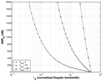
Figure 1: Signal-to-noise ratio threshold $\mathrm{SNR}_{\mathrm{th}}$ that describes the boundary between logarithmic and double-logarithmic capacity growths. We plot results for a fading channel with stationarity time $\delta_{\mathrm{stat}}\in\{1,10,100\}$ (in multiples of wavelength). The normalized Doppler bandwidth $\nu_{\mathrm{D}}$ is varied in the interval $(10^{-3},1/2)$.

For current communication systems like UMTS at $f_{C}=2\,$GHz the normalized Doppler bandwidth is $\nu_{\mathrm{D}}<0.02$. Thus, the double-logarithmic regime will not be reached. However, at higher carrier frequencies, e.g. $f_{C}=60\,$GHz or for underwater communication systems these bounds become more important.

VIII Conclusions

We have shown that the number of scatterers $P$ bounds the rank of the channel covariance matrix. The $\mathrm{SNR}$, the user’s velocity $v$, and the data block length $M$ define the usable rank of the channel subspace.

The usable channel subspace grows with the SNR. This growth in dimensionality must be taken into account for asymptotic capacity results in the high-SNR regime. For $P<M$ the asymptotic capacity grows logarithmically, while for $P\geq M$ a double-logarithmic growth is obtained.

Using results from the theory of time-concentrated and band-limited sequences, we are able to specify the SNR above which the double-logarithmic capacity region starts in the special case of a flat Doppler spectrum.

IX Acknowledgement

We would like to thank Joachim Wehinger and Christoph F. Mecklenbräuker for helpful discussions.

References

- [1] Y. Liang and V. V. Veervalli, “Capacity of noncoherent time-selective Rayleigh-fading channels,” IEEE Trans. Inform. Theory, vol. 50, no. 12, pp. 3095–3110, December 2004.
- [2] A. M. Sayeed, A. Sendonaris, and B. Aazhang, “Multiuser detection in fast-fading multipath environment,” IEEE J. Select. Areas Commun., vol. 16, no. 9, pp. 1691–1701, December 1998.
- [3] J. G. Proakis and D. G. Manolakis, Digital Signal Processing, 3rd ed. Prentice-Hall, 1996.
- [4] T. Zemen and C. F. Mecklenbräuker, “Time-variant channel estimation using discrete prolate spheroidal sequences,” IEEE Trans. Signal Processing, accepted for publication.
- [5] L. L. Scharf, Statistical Signal Processing: Detection, Estimation, and Time Series Analysis. Reading (MA), USA: Addison-Wesley Publishing Company, Inc., 1991.
- [6] D. Slepian, “Prolate spheroidal wave functions, Fourier analysis, and uncertainty - V: The discrete case,” The Bell System Technical Journal, vol. 57, no. 5, pp. 1371–1430, May-June 1978.
- [7] A. Lapidoth, “On the asymptotic capacity of stationary Gaussian fading channels,” IEEE Trans. Inform. Theory, vol. 51, no. 2, pp. 437–446, February 2005.
- [8] H. Hofstetter and G. Steinböck, “A geometry based stochastic channel model for MIMO systems,” in ITG Workshop on Smart Antennas, Munich, Germany, January 2004.
- [9] I. Viering and H. Hofstetter, “Potential of coefficient reduction in delay, space and time based on measurements,” in Conference on Information Sciences and Systems (CISS), Baltimore, USA, March 2003.
- [10] I. Viering, Analysis of Second Order Statistics for Improved Channel Estimation in Wireless Communications, ser. Fortschritts-Berichte VDI Reihe. Düsseldorf, Germany: VDI Verlag GmbH, 2003, no. 733.
- [11] T. Zemen, C. F. Mecklenbräuker, J. Wehinger, and R. R. Müller, “Iterative joint time-variant channel estimation and multi-user decoding for MC-CDMA,” IEEE Trans. Wireless Commun., revised.
- [12] M. Niedzwiecki, Identification of Time-Varying Processes. John Wiley & Sons, 2000.
- [13] A. Papoulis, Probability, Random Variables and Stochastic Processes. Singapore: McGraw-Hill, 1991.
- [14] A. Lapidoth, “On the high SNR capacity of stationary Gaussian fading channels,” in 41st Annual Allerton Conference on Communication, Control, and Computing, Monticello (IL), USA, October 2003.
- [15] T. Zemen, C. F. Mecklenbräuker, and R. R. Müller, “Time variant channel equalization for MC-CDMA via Fourier basis functions,” in Multi-Carrier Spread-Spectrum Workshop, Oberpaffenhofen, Germany, September 2003, pp. 451–454.
- [16] P. Schnitter, “Low-complexity equalization of OFDM in doubly selective channels,” IEEE Trans. Signal Processing, vol. 52, no. 4, pp. 1002–1011, April 2004.
- [17] H. J. Landau and H. O. Pollak, “Prolate spheroidal wave functions, Fourier analysis, and uncertainty - III: The dimension of the space of essentially time- and band-limited signals,” The Bell System Technical Journal, vol. 41, no. 4, pp. 1295–1336, July 1962.