Multiple Description Quantization Via Gram-Schmidt Orthogonalization

Abstract

The multiple description (MD) problem has received considerable attention as a model of information transmission over unreliable channels. A general framework for designing efficient multiple description quantization schemes is proposed in this paper. We provide a systematic treatment of the El Gamal-Cover (EGC) achievable MD rate-distortion region, and show that any point in the EGC region can be achieved via a successive quantization scheme along with quantization splitting. For the quadratic Gaussian case, the proposed scheme has an intrinsic connection with the Gram-Schmidt orthogonalization, which implies that the whole Gaussian MD rate-distortion region is achievable with a sequential dithered lattice-based quantization scheme as the dimension of the (optimal) lattice quantizers becomes large. Moreover, this scheme is shown to be universal for all i.i.d. smooth sources with performance no worse than that for an i.i.d. Gaussian source with the same variance and asymptotically optimal at high resolution. A class of low-complexity MD scalar quantizers in the proposed general framework also is constructed and is illustrated geometrically; the performance is analyzed in the high resolution regime, which exhibits a noticeable improvement over the existing MD scalar quantization schemes.

I Introduction

In the multiple description problem the total available bit rate is split between two channels and either channel may be subject to failure. It is desired to allocate rate and coded representations between the two channels, such that if one channel fails, an adequate reconstruction of the source is possible, but if both channels are available, an improved reconstruction over the single-channel reception results. The formal definition of the MD problem is as follows (also see Fig. 1).

Let $\{X(t)\}_{t=1}^{\infty}$ be an i.i.d. random process with $X(t)\sim p(x)$ for all $t$. Let $d(\cdot,\cdot):\mathcal{X}\times\mathcal{X}\rightarrow[0,d_{\max}]$ be a distortion measure.

Definition I.1

The quintuple $(R_{1},R_{2},D_{1},D_{2},D_{3})$ is called achievable if for all $\varepsilon>0$, there exist, for $n$ sufficiently large, encoding functions:

$$f_{i}^{(n)}:\mathcal{X}^{n}\rightarrow\mathcal{C}_{i}^{(n)}\quad\log|\mathcal{C}_{i}^{(n)}|\leq n(R_{i}+\varepsilon)\quad i=1,2,$$

and decoding functions:

$$g^{(n)}_{i}:\ \mathcal{C}_{i}^{(n)}\rightarrow\mathcal{X}^{n}\quad i=1,2$$

$$g^{(n)}_{3}:\ \mathcal{C}_{1}^{(n)}\times\mathcal{C}_{2}^{(n)}\rightarrow\mathcal{X}^{n}$$

such that for $\mathbf{\hat{X}}_{i}=g^{(n)}_{i}(f^{(n)}_{i}(\mathbf{X})),i=1,2$, and for $\mathbf{\hat{X}}_{3}=g^{(n)}_{3}(f^{(n)}_{1}(\mathbf{X}),f^{(n)}_{2}(\mathbf{X}))$,

$$\frac{1}{n}\mathbb{E}\sum\limits_{t=1}^{n}d(X(t),\hat{X}_{i}(t))<D_{i}+\varepsilon\quad i=1,2,3.$$

The MD rate-distortion region, denoted by $\mathcal{Q}$, is the set of all achievable quintuples.

In this paper the encoding functions $f^{(n)}_{1}$ and $f^{(n)}_{2}$ are referred to as encoder 1 and encoder 2, respectively. Similarly, decoding functions $g^{(n)}_{1}$, $g^{(n)}_{2}$ and $g^{(n)}_{3}$ are referred to as decoder 1, decoder 2, and decoder 3, respectively. It should be emphasized that in a real system, encoders 1 and 2 are just two different encoding functions of a single encoder while decoders 1, 2 and 3 are different decoding functions of a single decoder. Alternatively, in the MD literature decoders 1 and 2 are sometimes referred to as the side decoders because of their positions in Fig. 1, while decoder 3 is referred to as the central decoder.

\psfrag{x}[r]{$\mathbf{X}$}\psfrag{xhat1}[l]{$\mathbf{\hat{X}}_{1}$}\psfrag{xhat2}[l]{$\mathbf{\hat{X}}_{2}$}\psfrag{xhat3}[l]{$\mathbf{\hat{X}}_{3}$}\psfrag{en1}[c]{Encoder $1$}\psfrag{en2}[c]{Encoder $2$}\psfrag{r1}[c]{$R_{1}$}\psfrag{r2}[c]{$R_{2}$}\psfrag{de1}[c]{Decoder $1$}\psfrag{de2}[c]{Decoder $2$}\psfrag{de3}[c]{Decoder $3$}\includegraphics[scale={1}]{IT-multidescription}

Figure 1: Encoder and decoder diagram for multiple descriptions.

Early contributions to the MD problem can be found in [1, 2, 3, 4]. The first general result was El Gamal and Cover’s achievable region.

Definition I.2 (EGC region)

For random variables $U_{1},U_{2}$ and $U_{3}$ jointly distributed with the generic source variable $X$ via conditional distribution $p(u_{1},u_{2},u_{3}|x)$, let

$$\mathcal{R}(U_{1},U_{2},U_{3})=\left\{(R_{1},R_{2}):R_{1}+R_{2}\geq I(X;U_{1},U_{2},U_{3})+I(U_{1};U_{2}),R_{i}\geq I(X;U_{i}),i=1,2\right\}.$$

Let

$$\mathcal{Q}(U_{1},U_{2},U_{3})=\left\{(R_{1},R_{2},D_{1},D_{2},D_{3}):(R_{1},R_{2})\in\mathcal{R}(U_{1},U_{2},U_{3}),\exists\hat{X}_{i}=g_{i}(U_{i})\mbox{ with }\mathbb{E}d(X,\hat{X}_{i})\leq D_{i},i=1,2,3\right\}.$$

The EGC region is then defined as

$$\mathcal{Q}_{EGC}=\mbox{conv}\left(\bigcup\limits_{p(u_{1},u_{2},u_{3}|x)}\mathcal{Q}(U_{1},U_{2},U_{3})\right),$$

where $\mbox{conv}(\mathcal{S})$ denotes the convex hull of $\mathcal{S}$ for any set $\mathcal{S}$ in the Euclidean space.

It was proved in [5] that $\mathcal{Q}_{EGC}\subseteq\mathcal{Q}$. Ozarow [3] showed that $\mathcal{Q}_{EGC}=\mathcal{Q}$ for the quadratic Gaussian source. Ahlswede [6] showed that the EGC region is also tight for the “no excess sum-rate” case. Zhang and Berger [7] constructed a counterexample for which $\mathcal{Q}_{EGC}\subsetneqq\mathcal{Q}$. Further results can be found in [8, 9, 10, 11, 12, 13, 14]. The MD problem has also been generalized to the $n$-channel case [15, 16], but even the quadratic Gaussian case is far from being completely understood. The extension of the MD problem to the distributed source coding scenario has been considered in [17, 18], where the problem is again widely open.

The first constructive method to generate multiple descriptions is the multiple description scalar quantization (MDSQ), which was proposed by Vaishampayan [19, 20]. The key component of this method is the index assignment, which maps an index to an index pair as the two descriptions. However, the design of the index assignment turns out to be a difficult problem. Since optimal solution cannot be found efficiently, Vaishampayan [19] provided several heuristic methods to construct balanced index assignments which are not optimal but likely to perform well. The analysis of this class of balanced quantizers reveals that asymptotically (in rate) it is 3.07 dB away from the rate-distortion bound [21] in terms of central and side distortion product, when a uniform central quantizer is used; this granular distortion gap can be reduced by 0.4 dB when the central quantizer cells are better optimized [22]. The design of balanced index assignment was recently more thoroughly addressed in [23] from an algorithm perspective, and the index assignments for more than two description appeared in [24]. Other methods have also been proposed to optimize the index assignments [25, 26].

The framework of MDSQ was later extended to multiple description lattice vector quantization (MDLVQ) for balanced descriptions in [27] and for the asymmetric case in [28]. The design relies heavily on the choice of lattice/sublattice structure to facilitate the construction of index assignments. The analysis on these quantizers shows that the constructions are high-resolution optimal in asymptotically high dimensions; however, in lower dimension, optimization of the code-cells can also improve the high-resolution performance [29][30]. The major difficulty in constructing both MDSQ and MDLVQ is to find good index assignments, and thus it would simplify the overall design significantly if the component of index assignment can be eliminated altogether.

Frank-Dayan and Zamir [31] proposed a class of MD schemes which use entropy-coded dithered lattice quantizers (ECDQs). The system consists of two independently dithered lattice quantizers as the two side quantizers, with a possible third dithered lattice quantizer to provide refinement information for the central decoder. It was found that even with the quadratic Gaussian source, this system is only optimal in asymptotically high dimensions for the degenerate cases such as successive refinement and the “no excess marginal-rate” case, but not optimal in general. The difficulty lies in generating dependent quantization errors of two side quantizers to simulate the Gaussian multiple description test channel. Several possible improvements were provided in [31], but the problem remains unsolved.

The method of MD coding using correlating transforms was first proposed by Orchard, Wang, Vaishampayan, and Reibman [32, 33], and this technique has then been further developed in [34] and [35]. However, the transform-based approach is mainly designed for vector sources, and it is most suitable when the redundancy between the descriptions is kept relatively low.

In this paper we provide a systematic treatment of the El Gamal-Cover (EGC) achievable MD rate-distortion region and show it can be decomposed into a simplified-EGC (SEGC) region and an superimposed refinement operation. Furthermore, any point in the SEGC region can be achieved via a successive quantization scheme along with quantization splitting. For the quadratic Gaussian case, the MD rate-distortion region is the same as the SEGC region, and the proposed scheme has an intrinsic connection with the Gram-Schmidt orthogonalization method. Thus we use single-description ECDQs, with independent subtractive dithers as building blocks for this MD coding scheme, by which the difficulty of generating dependent quantization errors is circumvented. Analytical expressions for the rate-distortion performance of this system are then derived for general sources, and compared to the optimal rate regions at both high and low lattice dimensions.

The proposed scheme is conceptually different from those in [31], and it can achieve the whole Gaussian MD rate-distortion region as the dimension of the (optimal) lattice quantizers becomes large, unlike the method proposed in [31]. From a construction perspective, the new MD coding system can be realized by 2-3 conventional lattice quantizers along with some linear operations, and thus it is considerably simpler than MDSQ and MDLVQ by removing the index assignment and the reliance on the lattice/sublattice structure. Though the proposed coding scheme suggests many possible implementations of practical quantization methods, the focus of this article is on the information theoretic framework; thus instead of providing detailed designs of quantizers, a geometric interpretation of the scalar MD quantization scheme is given as an illustration to connect the information theoretic description of coding scheme and its practical counterpart.

The remainder of this paper is divided into 6 sections. In Section II, ECDQ and the Gram-Schmidt orthogonalization method are breifly reviewed and a connection between the successive quantization scheme and the Gram-Schmidt orthogonalization method is established. In Section III we present a systematic treatment of the EGC region and show the sufficiency of a successive quantization scheme along with quantization splitting. In Section IV the quadratic Gaussian case is considered in more depth. In Section V the proposed scheme based on ECDQ is shown to be universal for all i.i.d. smooth sources with performance no worse than that for an i.i.d. Gaussian source with the same variance and asymptotically optimal at high resolution. A geometric interpretation of the scalar MD quantization scheme in our framework is given in Section VI. Some further extensions are suggested in Section VII, which also serves as the conclusion. Throughout, we use boldfaced letters to indicate ($n$-dimensional) vectors, capital letters for random objects, and small letters for their realizations. For example, we let $\mathbf{X}=(X(1),\cdots,X(n))^{T}$ and $\mathbf{x}=(x(1),\cdots,x(n))^{T}$.

II Entropy-Coded Dithered Quantization and Gram-Schmidt Orthogonalization

In this section, we first give a brief review of ECDQ, and then explain the difficulty of applying ECDQ directly to the MD problem. As a method to resolve this difficulty, the Gram-Schmidt orthogonalization is introduced and a connection between the sequential (dithered) quantization and the Gram-Schmidt orthogonalization is established. The purpose of this section is two-fold: The first is to review related results on ECDQ and the Gram-Schmidt orthogonalization and show their connection, while the second is to explicate the intuition that motivated this work.

II-A Review of Entropy-Coded Dithered Quantization

Some basic definitions and properties of ECDQ from [31] are quoted below. More detailed discussion and derivation can be found in [36, 37, 38, 39].

An $n$-dimensional lattice quantizer is formed from a lattice $\mathbf{L}_{n}$. The quantizer $Q_{n}(\cdot)$ maps each vector $\mathbf{x}\in\mathcal{R}^{n}$ into the lattice point $\mathbf{l}_{i}\in\mathbf{L}_{n}$ that is nearest to $\mathbf{x}$. The region of all $n$-vectors mapped into a lattice point $\mathbf{l}_{i}\in\mathbf{L}_{n}$ is the Voronoi region

$$V(\mathbf{l}_{i})=\left\{\mathbf{x}\in\mathcal{R}^{n}:||\mathbf{x}-\mathbf{l}_{i}||\leq||\mathbf{x}-\mathbf{l}_{j}||,\forall j\neq i\right\}.$$

The dither $\mathbf{Z}$ is an $n$-dimensional random vector, independent of the source, and uniformly distributed over the basic cell $V_{0}$ of the lattice which is the Voronoi region of the lattice point $\mathbf{0}$. The dither vector is assumed to be available to both the encoder and the decoder. The normalized second moment $G_{n}$ of the lattice characterizes the second moment of the dither vector

$$\frac{1}{n}\mathbb{E}||\mathbf{Z}||^{2}=G_{n}V^{2/n},$$

where $V$ denotes the volume of $V_{0}$. Both the entropy encoder and the decoder are conditioned on the dither sample $\mathbf{Z}$; furthermore, the entropy coder is assumed to be ideal. The lattice quantizer with dither represents the source vector $\mathbf{X}$ by the vector $\mathbf{W}=Q_{n}(\mathbf{X}+\mathbf{Z})-\mathbf{Z}$. The resulting properties of the ECDQ are as follows.

1. The quantization error vector $\mathbf{W}-\mathbf{X}$ is independent of $\mathbf{X}$ and is distributed as $-\mathbf{Z}$. In particular, the mean-squared quantization error is given by the second moment of the dither, independently of the source distribution, i.e.,

   $$\frac{1}{n}\mathbb{E}||\mathbf{W}-\mathbf{X}||^{2}=\frac{1}{n}\mathbb{E}||\mathbf{Z}||^{2}=G_{n}V^{2/n}.$$

2. The coding rate of the ECDQ is equal to the mutual information between the input and output of an additive noise channel $\mathbf{Y}=\mathbf{X}+\mathbf{N}$, where $\mathbf{N}$, the channel’s noise, has the same probability density function as $-\mathbf{Z}$ (see Fig. 2) ,

   $$H(Q_{n}(\mathbf{X}+\mathbf{Z})|\mathbf{Z})=I(\mathbf{X};\mathbf{Y})=h(\mathbf{Y})-h(\mathbf{N}).$$

3. For optimal lattice quantizers, i.e., lattice quantizers with the minimal normalized second moment $G_{n}$, the autocorrelation of the quantizer noise is “white” , i.e., $\mathbb{E}\mathbf{Z}\mathbf{Z}^{T}=\sigma^{2}I_{n}$ where $I_{n}$ is the $n\times n$ identity matrix, $\sigma^{2}=G^{opt}_{n}V^{2/n}$ is the second moment of the lattice, and

   $$G^{opt}_{n}=\min\limits_{Q_{n}(\cdot)}\frac{\int_{V_{0}}||\mathbf{x}||^{2}\mbox{d}\mathbf{x}}{nV^{1+\frac{2}{n}}}$$

   is the minimal normalized second moment of an $n$-dimensional lattice.

\psfrag{x}[c]{$\mathbf{X}$}\psfrag{y}[c]{$\mathbf{Y}$}\psfrag{z}[c]{$\mathbf{Z}$}\psfrag{-z}[c]{$-\mathbf{Z}$}\psfrag{q}[c]{$Q_{n}(\cdot)$}\psfrag{e}[c]{E}\psfrag{d}[c]{D}\psfrag{r}[c]{$R$}\psfrag{n}[c]{$\mathbf{N}=-\mathbf{Z}$}\psfrag{sim}[c]{$\sim$}\psfrag{ecdq}[c]{ECDQ}\includegraphics[scale={1}]{IT-ecdq}

Figure 2: ECDQ and its equivalent additive-noise channel.

Consider the following problem to motivate the general result. Suppose a quantization system is needed with input $X_{1}$ and outputs $(X_{2},\cdots,X_{M})$ such that the quantization errors $X_{i}-X_{1}$, $i=2,\cdots,M$, are correlated with each other in a certain predetermined way, but are uncorrelated with $X_{1}$. Seemingly, $M-1$ quantizers may be used, each with $X_{1}$ as the input and $X_{i}$ as the output for some $i$, $i=2,\cdots,M$. By property 1) of ECDQ, if dithers are introduced, the quantization errors are uncorrelated (actually independent) of the input of the quantizer. However, it is difficult to make the quantization errors of these $M-1$ quantizers correlated in the desired manner. One may expect it to be possible to correlate the quantization errors by simply correlating the dithers of different quantizers, but this turns out to be not true as pointed out in [31]. Next, we present a solution to this problem by exploiting the relationship between the Gram-Schmidt orthogonalization and sequential (dithered) quantization.

II-B Gram-Schmidt Orthogonalization

In order to facilitate the treatment, the problem is reformulated in an equivalent form: Given $X^{M}_{1}$ with an arbitrary covariance matrix, construct a quantization system with $\widetilde{X}_{1}$ as the input and $(\widetilde{X}_{2},\cdots,\widetilde{X}_{M})$ as the outputs such that the covariance matrices of $X^{M}_{1}$ and $\widetilde{X}^{M}_{1}$ are the same.

Let $\mathcal{H}_{s}$ denote the set of all finite-variance, zero-mean, real scalar random variables. It is well known [40, 41] that $\mathcal{H}_{s}$ becomes a Hilbert space under the inner product mapping

$$\langle X,Y\rangle=\mathbb{E}(XY):\mathcal{H}_{s}\times\mathcal{H}_{s}\rightarrow\mathcal{R}.$$

The norm induced by this inner product is

$$\|X\|^{2}=\langle X,X\rangle=\mathbb{E}X^{2}.$$

For $X^{M}_{1}=(X_{1},\cdots,X_{M})^{T}$ with $X_{i}\in\mathcal{H}_{s}$, $i=1,\cdots,M$, the Gram-Schmidt orthogonalization can be used to construct an orthogonal basis $B^{M}_{1}=(B_{1},\cdots,B_{M})^{T}$ for $X^{M}_{1}$. Specifically, the Gram-Schmidt orthogonalization proceeds as follows:

$$B_{1} = X_{1},$$

$$B_{i} = X_{i}-\sum\limits_{j=1}^{i-1}\frac{\langle X_{i},B_{j}\rangle}{\|B_{j}\|^{2}}B_{j}$$

$$= X_{i}-\sum\limits_{j=1}^{i-1}\frac{\mathbb{E}(X_{i}B_{j})}{\mathbb{E}B^{2}_{j}}B_{j},\quad i=2,\cdots,M.$$

Note: $\frac{\mathbb{E}(X_{i}B_{j})}{\mathbb{E}B^{2}_{j}}$ can assume any real number if $B_{j}=0$. Alternatively, $B^{M}_{1}$ can also be computed using the method of linear estimation. Let $K_{X^{m}_{1}}$ denote the covariance matrix of $(X_{1},\cdots,X_{m})^{T}$ and let $K_{X_{m}X_{1}^{m-1}}=\mathbb{E}[X_{m}(X_{1},\cdots,X_{m-1})^{T}]$, then

$$B_{1} = X_{1},$$ (1)

$$B_{i} = X_{i}-K_{i-1}X^{i-1}_{1},\quad i=2,\cdots,M.$$ (2)

Here $K_{i-1}\in\mathcal{R}^{1\times(i-1)}$ is a row vector satisfying $K_{i-1}K_{X^{i-1}_{1}}=K_{X_{i}X^{i-1}_{1}}$. When $K_{X^{i-1}_{1}}$ is invertible, $K_{i-1}$ is uniquely given by $K_{X_{i}X^{i-1}_{1}}K^{-1}_{X^{i-1}_{1}}$. The product $K_{i-1}X^{i-1}_{1}$ is the linear MMSE estimate of $X_{i}$ given $X^{i-1}_{1}$, and $\mathbb{E}B^{2}_{i}$ is its corresponding linear MMSE estimation error.

The Gram-Schmidt orthogonalization is closely related to the $LDL^{T}$ factorization. That is, if all leading minors of $K_{X^{M}_{1}}$ are nonzero, then there exists a unique factorization such that $K_{X^{M}_{1}}=LDL^{T}$, where $D$ is diagonal, and $L$ is lower triangular with unit diagonal. Specifically, $D=\mbox{diag}\left\{\|B_{1}\|^{2},\cdots,\|B_{M}\|^{2}\right\}$ and

$$L = \begin{pmatrix}1&&&&\\ \frac{\langle X_{2},B_{1}\rangle}{\|B_{1}\|^{2}}&1&&&\\ \frac{\langle X_{3},B_{1}\rangle}{\|B_{1}\|^{2}}&\frac{\langle X_{3},B_{2}\rangle}{\|B_{2}\|^{2}}&1&&\\ \vdots&\vdots&\vdots&\ddots&\\ \frac{\langle X_{L},B_{1}\rangle}{\|B_{1}\|^{2}}&\frac{\langle X_{L},B_{2}\rangle}{\|B_{2}\|^{2}}&\frac{\langle X_{L},B_{3}\rangle}{\|B_{3}\|^{2}}&\cdots&1\end{pmatrix}.$$

$B^{M}_{1}=L^{-1}X^{M}_{1}$ is sometimes referred to as the innovation process [40].

In the special case in which $X^{M}_{1}$ are jointly Gaussian, the elements of $B^{M}_{1}$ are given by

$$B_{1} = X_{1},$$

$$B_{i} = X_{i}-\mathbb{E}(X_{i}|X^{i-1}_{1})$$

$$= X_{i}-\sum\limits_{j=1}^{i-1}\mathbb{E}(X_{i}|B_{j}),\quad i=2,\cdots,M,$$

and $B^{M}_{1}$ are zero-mean, independent and jointly Gaussian. Moreover, since $X^{i}_{1}$ is a deterministic function of $B^{i}_{1}$, it follows that $B^{M}_{i+1}$ is independent of $X^{i}_{1}$, for $i=1,\cdots,M-1$. Note: For $i=2,\cdots,M$, $\mathbb{E}(X_{i}|X^{i-1}_{1})$ (or $\sum_{j=1}^{i-1}\mathbb{E}(X_{i}|B_{j})$) is a sufficient statistic for estimation of $X_{i}$ from $X^{i-1}_{1}$ (or $B^{i-1}_{1}$); $\mathbb{E}(X_{i}|X^{i-1}_{1})$ (or $\sum_{j=1}^{i-1}\mathbb{E}(X_{i}|B_{j})$) also is the MMSE estimate of $X_{i}$ given $X^{i-1}_{1}$ (or $B^{i-1}_{1}$) and $\mathbb{E}B^{2}_{i}$ is the MMSE estimation error.

We now show that one can construct a sequential quantization system with $X_{1}$ as the input to generate a zero-mean random vector $\widetilde{X}^{M}_{1}=(\widetilde{X}_{1},\widetilde{X}_{2},\cdots,\widetilde{X}_{M})^{T}$ whose covariance matrix is also $K_{X^{M}_{1}}$. Let $X^{M}_{1}$ be a zero-mean random vector with covariance matrix $K_{X^{M}_{1}}$. By (1) and (2), it is true that

$$X_{1} = B_{1},$$ (3)

$$X_{i} = K_{i-1}X^{i-1}_{1}+B_{i},\quad i=2,\cdots,M.$$ (4)

Assume that $B_{i}\neq 0$ for $i=2,\cdots,M$. Let $Q_{i,1}(\cdot)$ be a scalar lattice quantizer with step size $\Delta_{i}=\sqrt{12\mathbb{E}B^{2}_{i+1}}$, $i=1,2,\cdots,M-1$. Let the dither $Z_{i}\sim\mathcal{U}(-\Delta_{i}/2,\Delta_{i}/2)$ be a random variable uniformly distributed over the basic cell of $Q_{i,1}$, $i=1,2,\cdots,M-1$. Note: the second subscript $n$ of $Q_{i,n}$ denotes the dimension of the lattice quantizer. In this case $n=1$, so it is a scalar quantizer.

Suppose $(X_{1},Z_{1},\cdots,Z_{M-1})$ are independent. Define

$$\widetilde{X}_{1} = X_{1},$$

$$\widetilde{X}_{i} = Q_{i-1,1}\left(K_{i-1}\widetilde{X}^{i-1}_{1}+Z_{i-1}\right)-Z_{i-1},\quad i=2,\cdots,M.$$

By property 2) of the ECDQ, we have

$$\widetilde{X}_{1} = X_{1},$$ (5)

$$\widetilde{X}_{i} = K_{i-1}\widetilde{X}^{i-1}_{1}+N_{i},\quad i=2,\cdots,M,$$ (6)

where $N_{i}\sim\mathcal{U}(\Delta_{i}/2,\Delta_{i}/2)$ with $\mathbb{E}N^{2}_{i}=\mathbb{E}B^{2}_{i+1}$, $i=1,\cdots,M-1$, and $(X_{1},N_{1},\cdots,N_{M})$ are independent. By comparing (3), (4) and (5), (6), it is straightforward to verify that $X^{M}_{1}$ and $\widetilde{X}^{M}_{1}$ have the same covariance matrix.

Since $\mathbb{E}B^{2}_{i}$ $(i=2,\cdots,M)$ are not necessarily the same, it follows that the quantizers $Q_{i,1}(\cdot)$ $(i=1,\cdots,M-1)$ are different in general. But by incorporating linear pre- and post-filters [38], all these quantizers can be made identical. Specifically, given a scalar lattice quantizer $Q_{1}(\cdot)$ with step size $\Delta$, let the dither $Z^{\prime}_{i}\sim\mathcal{U}(-\Delta/2,\Delta/2)$ be a random variable uniformly distributed over the basic cell of $Q_{1}$, $i=1,2,\cdots,M-1$. Suppose $(X_{1},Z^{\prime}_{1},\cdots,Z^{\prime}_{M-1})$ are independent. Define

$$\overline{X}_{1} = X_{1},$$

$$\overline{X}_{i} = a_{i-1}\left[Q_{1}\left(\frac{1}{a_{i-1}}K_{i-1}\overline{X}^{i-1}_{1}+Z^{\prime}_{i-1}\right)-Z^{\prime}_{i-1}\right],\quad i=2,\cdots,M,$$

where $a_{i}=\pm\sqrt{\frac{12\mathbb{E}B^{2}_{i+1}}{\Delta^{2}}}$, $i=1,2,\cdots,M-1$. By property 2) of the ECDQ, it is again straightforward to verify that $X^{M}_{1}$ and $\overline{X}^{M}_{1}$ have the same covariance matrix. Essentially by introducing the prefilter $\frac{1}{a_{i}}$ and the postfilter $a_{i}$, the quantizer $Q_{1}(\cdot)$ is converted to the quantizer $Q_{i,1}(\cdot)$ for which

$$Q_{i,1}(x)=a_{i}Q_{1}(\frac{x}{a_{i}}).$$

This is referred to as the shaping [37] of the quantizer $Q_{1}(\cdot)$ by $a_{i}$. In the case where $\Delta^{2}=12$, we have $\mathbb{E}(Z^{\prime}_{i})^{2}=1$, $i=1,\cdots,M-1$, and the constructed sequential (dithered) quantization system can be regarded as a simulation of Gram-Schmidt orthonormalization.

If $B_{i}=0$ for some $i$, then $\widetilde{X}_{i}=K_{i-1}\widetilde{X}^{i-1}_{1}$ (or $\overline{X}_{i}=K_{i-1}\overline{X}^{i-1}_{1}$) and therefore no quantization operation is needed to generate $\widetilde{X}_{i}$ (or $\overline{X}_{i}$ ) from $\widetilde{X}^{i-1}_{1}$ (or $\overline{X}^{i-1}_{1}$).

The generalization of the correspondence between the Gram-Schmidt orthogonalization and the sequential (dithered) quantization to the vector case is straightforward; see Appendix I.

III Successive Quantization and Quantization Splitting

In this section, an information-theoretic analysis of the EGC region is provided. Two coding schemes, namely successive quantization and quantization splitting, are subsequently introduced. Together with Gram-Schmidt orthogonalization, they are the main components of the quantization schemes that will be presented in the next two sections.

III-A An information theoretic analysis of the EGC region

Rewrite $\mathcal{R}(U_{1},U_{2},U_{3})$ in the following form:

$$\mathcal{R}(U_{1},U_{2},U_{3})=\left\{(R_{1},R_{2}):R_{1}+R_{2}\geq I(X;U_{1},U_{2})+I(U_{1};U_{2})+I(X;U_{3}|U_{1},U_{2}),R_{i}\geq I(X;U_{i}),i=1,2\right\}.$$

Without loss of generality, assume that $X\rightarrow U_{3}\rightarrow(U_{1},U_{2})$ form a Markov chain since otherwise $U_{3}$ can be replaced by $\widetilde{U}_{3}=(U_{1},U_{2},U_{3})$ without affecting the rate and distortion constraints. Therefore $U_{3}$ can be viewed as a fine description of $X$ and $(U_{1},U_{2})$ as coarse descriptions of $X$. The term $I(X,U_{3}|U_{1},U_{2})$ is the rate used for the superimposed refinement from the pair of coarse descriptions $(U_{1},U_{2})$ to the fine description $U_{3}$; in general, this refinement rate is split between the two channels. Since description refinement schemes have been studied extensively in the multiresolution or layered source coding scenario and are well-understood, this operation can be separated from other parts of the EGC scheme.

Definition III.1 (SEGC region)

For random variables $U_{1}$ and $U_{2}$ jointly distributed with the generic source variable $X$ via conditional distribution $p(u_{1},u_{2}|x)$, let

$$\mathcal{R}(U_{1},U_{2})=\left\{(R_{1},R_{2}):R_{1}+R_{2}\geq I(X;U_{1},U_{2})+I(U_{1};U_{2}),R_{i}\geq I(X;U_{i}),i=1,2\right\}.$$

Let

$$\mathcal{Q}(U_{1},U_{2})=\left\{(R_{1},R_{2},D_{1},D_{2},D_{3}):(R_{1},R_{2})\in\mathcal{R}(U_{1},U_{2}),\exists\hat{X}_{1}=g_{1}(U_{1}),\hat{X}_{2}=g_{2}(U_{2}),\hat{X}_{3}=g_{3}(U_{1},U_{2})\right.$$

$$\left.\mbox{ with }\mathbb{E}d(X,\hat{X}_{i})\leq D_{i},i=1,2,3\right\}.$$

The SEGC region is defined as

$$\mathcal{Q}_{SEGC}=\mbox{conv}\left(\bigcup\limits_{p(u_{1},u_{2}|x)}\mathcal{Q}(U_{1},U_{2})\right).$$

The SEGC region first appeared in [1] and was attributed to El Gamal and Cover. It was shown in [7] that $\mathcal{Q}_{SEGC}\subseteq\mathcal{Q}_{EGC}$.

Using the identity

$$I(A;BC)=I(A;B)+I(A;C)+I(B;C|A)-I(B;C),$$

$\mathcal{R}(U_{1},U_{2})$ can be written as

$$\mathcal{R}(U_{1},U_{2})=\left\{(R_{1},R_{2}):R_{1}+R_{2}\geq I(X;U_{1})+I(X;U_{2})+I(U_{1};U_{2}|X),R_{i}\geq I(X;U_{i}),i=1,2\right\}.$$

The typical shape of $\mathcal{R}(U_{1},U_{2})$ is shown in Fig. 3.

\psfrag{r1}[r]{$R_{1}$}\psfrag{r2}[r]{$R_{2}$}\psfrag{v1}[r]{$V_{1}$}\psfrag{v2}[c]{$V_{2}$}\includegraphics[scale={0.8}]{ciss05-RDregion}

Figure 3: The shape of $\mathcal{R}(U_{1},U_{2})$.

It is noteworthy that $\mathcal{R}(U_{1},U_{2})$ resembles Marton’s achievable region [42] for a two-user broadcast channel. This is not surprising since the proof of the EGC theorem relies heavily on the results in [43] which were originally for a simplified proof of Marton’s coding theorem for the discrete memoryless broadcast channel. Since the corner points of Marton’s region can be achieved via a relatively simple coding scheme due to Gel’fand and Pinsker [44], which for the Gaussian case becomes Costa’s dirty paper coding [45], it is natural to conjecture that simple quantization schemes may exist for the corner points of $\mathcal{R}(U_{1},U_{2})$. This conjecture turns out to be correct as will be shown below.

Since $I(U_{1};U_{2}|X)\geq 0$, the sum-rate constraint in $\mathcal{R}(U_{1},U_{2})$ is always effective. Thus

$$\left\{(R_{1},R_{2}):R_{1}+R_{2}=I(X;U_{1})+I(X;U_{2})+I(U_{1};U_{2}|X),R_{i}\geq I(X;U_{i}),i=1,2\right\}$$

will be called the dominant face of $\mathcal{R}(U_{1},U_{2})$. Any rate pair inside $\mathcal{R}(U_{1},U_{2})$ is inferior to some rate pair on the dominant face in terms of compression efficiency. Hence, in searching for the optimal scheme, attention can be restricted to rate pairs on the dominant face without loss of generality. The dominant face of $\mathcal{R}(U_{1},U_{2})$ has two vertices $V_{1}$ and $V_{2}$. Let $(R_{1}(V_{i}),R_{2}(V_{i}))$ denote the coordinates of vertex $V_{i}$, $i=1,2$, then

1. $V_{1}$: $R_{1}(V_{1})=I(X;U_{1})$, $R_{2}(V_{1})=I(X,U_{1};U_{2})$;

2. $V_{2}$: $R_{1}(V_{2})=I(X,U_{2};U_{1})$, $R_{2}(V_{2})=I(X;U_{2})$.

The expressions of these two vertices directly lead to the following successive quantization scheme. By symmetry, we shall only consider $V_{1}$.

III-B Successive Quantization Scheme

The successive quantization scheme is given as follows:

1. Codebook Generation: Encoder 1 independently generates $2^{n[I(X;U_{1})+\epsilon_{1}]}$ codewords $\{\mathbf{U}_{1}(j)\}_{j=1}^{2^{n[I(X;U_{1})+\epsilon_{1}]}}$ according to the distribution $\prod p(u_{1})$. Encoder 2 independently generates $2^{n[I(X,U_{1};U_{2})+\epsilon_{2}]}$ codewords $\{\mathbf{U}_{2}(k)\}_{k=1}^{2^{n[I(X,U_{1};U_{2})+\epsilon_{2}]}}$ according to the distribution $\prod p(u_{2})$.

2. Encoding Procedure: Given $\mathbf{X}$, encoder 1 finds the codeword $\mathbf{U}_{1}(j^{*})$ such that $\mathbf{U}_{1}(j^{*})$ is strongly typical with $\mathbf{X}$. Then encoder 2 finds the codeword $\mathbf{U}_{2}(k^{*})$ such that $\mathbf{U}_{2}(k^{*})$ is strongly typical with $\mathbf{X}$ and $\mathbf{U}_{1}(j^{*})$. Index $j^{*}$ is transmitted through channel 1 and index $k^{*}$ is transmitted through channel 2.

3. Reconstruction: Decoder $1$ reconstructs $\mathbf{\hat{X}}_{1}$ with $\hat{X}_{1}(t)=g_{1}(U_{1}(j^{*},t))$. Decoder $2$ reconstructs $\mathbf{\hat{X}}_{2}$ with $\hat{X}_{2}(t)=g_{2}(U_{2}(k^{*},t))$. Decoder $3$ reconstructs $\mathbf{\hat{X}}_{3}$ with $\hat{X}_{3}(t)=g_{3}(U_{1}(j^{*},t),U_{2}(k^{*},t))$. Here, $U_{1}(j^{*},t)$ and $U_{2}(k^{*},t)$ are the $t$-th entries of $\mathbf{U}_{1}(j^{*})$ and $\mathbf{U}_{2}(k^{*})$, respectively, $t=1,2,\cdots,n$.

It can be shown rigorously that

$$\frac{1}{n}\sum\limits_{t=1}^{n}\mathbb{E}d(X_{i}(t),\hat{X}_{i}(t)) \leq \mathbb{E}d(X,g_{i}(U_{i}))+\epsilon_{2+i},\quad i=1,2,$$

$$\frac{1}{n}\sum\limits_{t=1}^{n}\mathbb{E}d(X_{3}(t),\hat{X}_{3}(t)) \leq \mathbb{E}d(X,g_{3}(U_{1},U_{2}))+\epsilon_{5}$$

as $n$ goes to infinity and $\epsilon_{i}$ $(i=1,2,\cdots,5)$ can be made arbitrarily close to zero. The proof is conventional and thus is omitted.

For this scheme, encoder 1 does the encoding first and then encoder 2 follows. The main complexity of this scheme resides in encoder 2, since it needs to construct a codebook that covers the $(\mathbf{X},\mathbf{U}_{1})$-space instead of just the $\mathbf{X}$-space. Observe that, if a function $f(X,U_{1})=V$ can be found such that $V$ is a sufficient statistic for estimation $U_{2}$ from $(X,U_{1})$, i.e., $(X,U_{1})\rightarrow V\rightarrow U_{2}$ form a Markov chain, then

$$I(X,U_{1};U_{2})=I(V;U_{2}).$$

The importance of this observation is that encoder 2 then only needs to construct a codebook that covers the $\mathbf{V}$-space instead of the $(\mathbf{X},\mathbf{U}_{1})$-space. This is because the Markov lemma [46] implies that if $\mathbf{U}_{2}$ is jointly typical with $\mathbf{V}$, then $\mathbf{U}_{2}$ is jointly typical with $(\mathbf{X},\mathbf{U}_{1})$ with high probability. This observation turns out to be crucial for the quadratic Gaussian case.

We point out that the successive coding structure associated with the corner points of $\mathcal{R}(U_{1},U_{2})$ is not a special case in network information theory. Besides its resemblance to the successive Gel’fand-Pinsker coding structure associated with the corner points of the Marton’s region previously mentioned, other noteworthy examples include the successive decoding structure associated with the corner points of the Slepian-Wolf region [47] (and more generally, the Berger-Tung region [46, 48, 49]) and the corner points of the capacity region of the memoryless multiaccess channel [50, 51].

III-C Successive Quantization Scheme with Quantization Splitting

A straightforward method to achieve an arbitrary rate pair on the dominant face of $\mathcal{R}(U_{1},U_{2})$ is timesharing of coding schemes that achieve the two vertices. However, such a scheme requires four quantizers in general. Instead, the scheme based on quantization splitting introduced below needs only three quantizers. Before presenting it, we shall first prove the following theorem.

Theorem III.1

For any rate pair $(R_{1},R_{2})$ on the dominant face of $\mathcal{R}(U_{1},U_{2})$, there exists a random variable $U^{\prime}_{2}$ with $(X,U_{1})\rightarrow U_{2}\rightarrow U^{\prime}_{2}$ such that

$$R_{1} = I(X,U^{\prime}_{2};U_{1}),$$

$$R_{2} = I(X;U^{\prime}_{2})+I(X,U_{1};U_{2}|U^{\prime}_{2}).$$

Similarly, there exists a random variable $U^{\prime}_{1}$ with $(X,U_{2})\rightarrow U_{1}\rightarrow U^{\prime}_{1}$ such that

$$R_{1} = I(X,U^{\prime}_{1})+I(X,\hat{X}_{2};U_{1}|U^{\prime}_{1}),$$

$$R_{2} = I(X,U^{\prime}_{1};U_{2}).$$

Before proceeding to prove this theorem, we make the following remarks.

• By the symmetry between the two forms, only the statement regarding the first form needs to be proved.

• Since $(X,U_{1})\rightarrow U_{2}\rightarrow U^{\prime}_{2}$ form a Markov chain, if $U^{\prime}_{2}$ is independent of $U_{2}$, then it must be independent of $(X,U_{1},U_{2})$ altogether. Then in this case,

  $$R_{1}=I(X;U_{1}),\quad R_{2}=I(X,U_{1};U_{2}),$$

  which are the coordinates of $V_{1}$.

• At the other extreme, letting $U^{\prime}_{2}$ be $U_{2}$ gives

  $$R_{1}=I(X,U_{2};U_{1}),\quad R_{2}=I(X,U_{2}),$$

  which are the coordinates of $V_{2}$.

Proof:

First construct a class of transition probabilities $p_{\epsilon}(u^{\prime}_{2}|u_{2})$ indexed by $\epsilon$ such that $I(U;U^{\prime}_{2})$ varies continuously from 0 to $H(U_{2})$ as $\epsilon$ changes from 0 to 1, with $(X,U_{1})\rightarrow U_{2}\rightarrow U^{\prime}_{2}$ holding for all the members of this class. It remains to show that

$$R_{1}+R_{2}=I(X,U_{1})+I(X;U_{2})+I(U_{1};U_{2}|X).$$

This is indeed true since

$$R_{1}+R_{2} = I(X,U^{\prime}_{2};U_{1})+I(X;U^{\prime}_{2})+I(X,U_{1};U_{2}|U^{\prime}_{2})$$

$$= I(X,U^{\prime}_{2};U_{1})+I(X;U^{\prime}_{2})+I(X;U_{2}|U^{\prime}_{2})+I(U_{1};U_{2}|X,U^{\prime}_{2})$$

$$= I(X,U_{2},U^{\prime}_{2};U_{1})+I(X;U_{2},U^{\prime}_{2}).$$

By the construction $(X,U_{1})\rightarrow U_{2}\rightarrow U^{\prime}_{2}$, it follows that

$$I(X,U_{2},U^{\prime}_{2};U_{1})+I(X;U_{2},U^{\prime}_{2})$$

$$= I(X,U_{2};U_{1})+I(X;U_{2})$$

$$= I(X,U_{1})+I(X;U_{2})+I(U_{1};U_{2}|X),$$

which completes the proof. ∎

The successive quantization scheme with quantization splitting is given as follows:

1. Codebook Generation: Encoder 1 independently generates $2^{n[I(X,U^{\prime}_{2};U_{1})+\epsilon^{\prime}_{1}]}$ codewords $\{\mathbf{U}_{1}(i)\}_{i=1}^{2^{n[I(X,U^{\prime}_{2};U_{1})+\epsilon^{\prime}_{1}]}}$ according to the marginal distribution $\prod p(u_{1})$. Encoder 2 independently generates $2^{n[I(X;U^{\prime}_{2})+\epsilon^{\prime}_{2}]}$ codewords $\{{\mathbf{U^{\prime}}_{2}}(j)\}_{j=1}^{2^{n[I(X;U^{\prime}_{2})+\epsilon^{\prime}_{2}]}}$ according to the marginal distribution $\prod p(u^{\prime}_{2})$. For each codeword ${\mathbf{U^{\prime}}_{2}}(j)$, encoder 2 independently generates $2^{n[I(X,U_{1};U_{2}|U^{\prime}_{2})+\epsilon^{\prime}_{3}]}$ codewords $\{{\mathbf{U}_{2}}(j,k)\}_{k=1}^{2^{n[I(X,U_{1};U_{2}|U^{\prime}_{2})+\epsilon^{\prime}_{3}]}}$ according to the conditional distribution $\prod\limits_{t}p(u_{2}|U^{\prime}_{2}(j,t))$. Here $U^{\prime}_{2}(j,t)$ is the $t$-th entry of $\mathbf{U^{\prime}}_{2}(j)$

2. Encoding Procedure: Given $\mathbf{X}$, encoder 2 finds the codeword ${\mathbf{U^{\prime}}_{2}}(j^{*})$ such that ${\mathbf{U^{\prime}}_{2}}(j^{*})$ is strongly typical with $\mathbf{X}$. Then encoder 1 finds the codeword $\mathbf{U}_{1}(i^{*})$ such that $\mathbf{U}_{1}(i^{*})$ is strongly typical with $\mathbf{X}$ and ${\mathbf{U^{\prime}}_{2}}(j^{*})$. Finally, encoder 2 finds the codeword ${\mathbf{U}_{2}}(j^{*},k^{*})$ such that $\mathbf{U}_{2}(j^{*},k^{*})$ is strongly typical with $\mathbf{X}$, $\mathbf{U}_{1}(i^{*})$ and ${\mathbf{U^{\prime}}_{2}}(j^{*})$. Index $i^{*}$ is transmitted through channel 1. Indices $j^{*}$ and $k^{*}$ are transmitted through channel 2.

3. Reconstruction: Decoder $1$ reconstructs $\mathbf{\hat{X}}_{1}$ with $\hat{X}_{1}(t)=g_{1}(U_{1}(i^{*},t))$. Decoder $2$ reconstructs $\mathbf{\hat{X}}_{2}$ with $\hat{X}_{2}(t)=g_{2}(U_{2}(j^{*},k^{*},t))$. Decoder $3$ reconstructs $\mathbf{\hat{X}}_{3}$ with $\hat{X}_{3}(t)=g_{3}(U_{1}(i^{*},t),U_{2}(j^{*},k^{*},t))$. Here $U_{1}(i^{*},t)$ is the $t$-th entry of $\mathbf{U}_{1}(i^{*})$ and $U_{2}(j^{*},k^{*},t)$ is the $t$-th entry of $\mathbf{U}_{2}(j^{*},k^{*})$, $t=1,2,\cdots,n$.

Again, it can be shown rigorously that

$$\frac{1}{n}\sum\limits_{t=1}^{n}\mathbb{E}d(X_{i}(t),\hat{X}_{i}(t)) \leq \mathbb{E}d(X,g_{i}(U_{i}))+\epsilon^{\prime}_{3+i},\quad i=1,2,$$

$$\frac{1}{n}\sum\limits_{t=1}^{n}\mathbb{E}d(X_{3}(t),\hat{X}_{3}(t)) \leq \mathbb{E}d(X,g_{3}(U_{1},U_{2}))+\epsilon^{\prime}_{6}$$

as $n$ goes to infinity and $\epsilon^{\prime}_{i}$ $(i=1,2,\cdots,6)$ can be made arbitrarily close to zero. The proof is standard, so the details are omitted.

This approach is a natural generalization of the successive quantization scheme for the vertices of $\mathcal{R}(U_{1},U_{2})$. $U^{\prime}_{2}$ can be viewed as a coarse description of $X$ and $U_{2}$ as a fine description of $X$. The idea of introducing an auxiliary coarse description to convert a joint coding scheme to a successive coding scheme has been widely used in the distributed source coding problems [52, 53, 54]. Similar ideas have also found application in multiaccess communications [55, 56, 57, 58].

IV The Gaussian Multiple Description Region

In this section we apply the general results in the preceding section to the quadratic Gaussian case. The Gaussian MD rate-distortion region is first analyzed to show that $\mathcal{Q}_{EGC}=\mathcal{Q}_{SEGC}$ in this case. Then, by incorporating the Gram-Schmidt orthogonalization with successive quantization and quantization splitting, a coding scheme that achieves the whole Gaussian MD region is presented.

IV-A An Analysis of the Gaussian MD Region

Let $\{X^{G}(t)\}_{t=1}^{\infty}$ be an i.i.d. Gaussian process with $X^{G}(t)\sim\mathcal{N}(0,\sigma^{2}_{X})$ for all $t$. Let $d(\cdot,\cdot)$ be the squared error distortion measure. For the quadratic Gaussian case, the MD rate-distortion region was characterized in [5, 3, 60]. Namely, $(R_{1},R_{2},D_{1},D_{2},D_{3})\in\mathcal{Q}$ if and only if

$$R_{i} \geq \frac{1}{2}\log\frac{\sigma^{2}_{X}}{D_{i}},\quad i=1,2,$$

$$R_{1}+R_{2} \geq \frac{1}{2}\log\frac{\sigma^{2}_{X}}{D_{3}}+\frac{1}{2}\log\psi(D_{1},D_{2},D_{3}),$$

where

$$\psi(D_{1},D_{2},D_{3})=\left\{\begin{array}[]{ll}1,\hskip 140.92627ptD_{3}<D_{1}+D_{2}-\sigma^{2}_{X}\\ \frac{\sigma^{2}_{X}D_{3}}{D_{1}D_{2}},\hskip 122.85876ptD_{3}>\left(\frac{1}{D_{1}}+\frac{1}{D_{2}}-\frac{1}{\sigma^{2}_{X}}\right)^{-1}\\ \frac{(\sigma^{2}_{X}-D_{3})^{2}}{(\sigma^{2}_{X}-D_{3})^{2}-[\sqrt{(\sigma^{2}_{X}-D_{1})(\sigma^{2}_{X}-D_{2})}-\sqrt{(D_{1}-D_{3})(D_{2}-D_{3})}]^{2}},\mbox{ o.w.}\\ \end{array}\right.$$

The case $D_{3}<D_{1}+D_{2}-\sigma^{2}_{X}$ and the case $D_{3}>\left(1/{D_{1}}+1/{D_{2}}-1/{\sigma^{2}_{X}}\right)^{-1}$ are degenerate. It is easy to verify that for any $(R_{1},R_{2},D_{1},D_{2},D_{3})\in\mathcal{Q}$ with $D_{3}<D_{1}+D_{2}-\sigma^{2}_{X}$, there exist $D^{*}_{1}\leq D_{1}$, $D^{*}_{2}\leq D_{2}$ such that $(R_{1},R_{2},D^{*}_{1},D^{*}_{2},D_{3})\in\mathcal{Q}$ and $D_{3}=D^{*}_{1}+D^{*}_{2}-\sigma^{2}_{X}$. Similarly, for any $(R_{1},R_{2},D_{1},D_{2},D_{3})\in\mathcal{Q}$ with $D_{3}>\left(1/{D_{1}}+1/{D_{2}}-1/{\sigma^{2}_{X}}\right)^{-1}$, there exist $D^{*}_{3}=\left(1/{D_{1}}+1/{D_{2}}-1/{\sigma^{2}_{X}}\right)^{-1}<D_{3}$ such that $(R_{1},R_{2},D_{1},D_{2},D^{*}_{3})\in\mathcal{Q}$. Henceforth we shall only consider the subregion when $\left(1/{D_{1}}+1/{D_{2}}-1/{\sigma^{2}_{X}}\right)^{-1}\geq D_{3}\geq D_{1}+D_{2}-\sigma^{2}_{X}$, for which $D_{1},D_{2}$ and $D_{3}$ all are effective.

Following the approach in [5], let

$$U_{1} = X^{G}+T_{0}+T_{1},$$ (8)

$$U_{2} = X^{G}+T_{0}+T_{2},$$ (9)

where $(T_{1},T_{2})$, $T_{0}$, $X$ are zero-mean, jointly Gaussian and independent, and $\mathbb{E}(T_{1}T_{2})=-\sigma_{T_{1}}\sigma_{T_{2}}$. Let $\hat{X}^{G}_{i}=\mathbb{E}(X^{G}|U_{i})=\alpha_{i}U_{i}$ $(i=1,2)$, and $\hat{X}^{G}_{3}=\mathbb{E}(X^{G}|U_{1},U_{2})=\beta_{1}U_{1}+\beta_{2}U_{2}$, where

$$\alpha_{i} = \frac{\sigma^{2}_{X}}{\sigma^{2}_{X}+\sigma^{2}_{T_{0}}+\sigma^{2}_{T_{i}}},\quad i=1,2,$$

$$\beta_{1} = \frac{\sigma^{2}_{X}\sigma_{T_{2}}}{(\sigma_{T_{1}}+\sigma_{T_{2}})(\sigma^{2}_{X}+\sigma^{2}_{T_{0}})},$$

$$\beta_{2} = \frac{\sigma^{2}_{X}\sigma_{T_{1}}}{(\sigma_{T_{1}}+\sigma_{T_{2}})(\sigma^{2}_{X}+\sigma^{2}_{T_{0}})}.$$

Set $\mathbb{E}(X^{G}-\hat{X}^{G}_{i})^{2}=D_{i}$, $i=1,2,3$; then

$$\sigma^{2}_{T_{0}} = \frac{D_{3}\sigma^{2}_{X}}{\sigma^{2}_{X}-D_{3}},$$ (10)

$$\sigma^{2}_{T_{i}} = \frac{D_{i}\sigma^{2}_{X}}{\sigma^{2}_{X}-D_{i}}-\frac{D_{3}\sigma^{2}_{X}}{\sigma^{2}_{X}-D_{3}},\quad i=1,2.$$ (11)

With these $\sigma^{2}_{T_{i}}$ $(i=0,1,2)$, it is straightforward to verify that

$$I(X^{G};U_{i}) = \frac{1}{2}\log\frac{\sigma^{2}_{X}+\sigma^{2}_{T_{0}}+\sigma^{2}_{T_{i}}}{\sigma^{2}_{T_{0}}+\sigma^{2}_{T_{i}}}$$

$$= \frac{1}{2}\log\frac{\sigma^{2}_{X}}{D_{i}}\quad i=1,2,$$

$$I(X^{G};U_{1})+I(X^{G};U_{2})+I(U_{1};U_{2}|X^{G}) = \frac{1}{2}\log\frac{\sigma^{2}_{X}+\sigma^{2}_{T_{0}}+\sigma^{2}_{T_{1}}}{\sigma^{2}_{T_{0}}+\sigma^{2}_{T_{1}}}+\frac{1}{2}\log\frac{\sigma^{2}_{X}+\sigma^{2}_{T_{0}}+\sigma^{2}_{T_{2}}}{\sigma^{2}_{T_{0}}+\sigma^{2}_{T_{2}}}$$

$$+\frac{1}{2}\log\frac{(\sigma^{2}_{T_{0}}+\sigma^{2}_{T_{1}})(\sigma^{2}_{T_{0}}+\sigma^{2}_{T_{2}})}{\sigma^{2}_{T_{0}}(\sigma_{T_{1}}+\sigma_{T_{2}})^{2}}$$

$$= \frac{1}{2}\log\frac{\sigma^{2}_{X}}{D_{3}}+\frac{1}{2}\log\psi(D_{1},D_{2},D_{3}).$$

Therefore, we have

$$\mathcal{R}^{G}(U_{1},U_{2}) \triangleq \left\{(R_{1},R_{2}):R_{1}+R_{2}\geq I(X^{G};U_{1})+I(X^{G};U_{2})+I(U_{1};U_{2}|X^{G}),R_{i}\geq I(X^{G};U_{i}),i=1,2\right\}$$ (12)

$$= \left\{(R_{1},R_{2}):R_{1}+R_{2}\geq\frac{1}{2}\log\frac{\sigma^{2}_{X}}{D_{3}}+\frac{1}{2}\log\psi(D_{1},D_{2},D_{3}),R_{i}\geq\frac{1}{2}\log\frac{\sigma^{2}_{X}}{D_{i}},i=1,2\right\}.$$

Hence for the quadratic Gaussian case,

$$\mathcal{Q}=\mathcal{Q}_{EGC}=\mathcal{Q}_{SEGC}$$

and there is no need to introduce $U_{3}$ (more precisely, $U_{3}$ can be represented as a deterministic function of $U_{1}$ and $U_{2}$).

The coordinates of the vertices $V^{G}_{1}$ and $V^{G}_{2}$ of $\mathcal{R}^{G}(U_{1},U_{2})$ can be computed as follows.

$$R_{1}(V^{G}_{1}) = \frac{1}{2}\log\frac{\sigma^{2}_{X}+\sigma^{2}_{T_{0}}+\sigma^{2}_{T_{1}}}{\sigma^{2}_{T_{0}}+\sigma^{2}_{T_{1}}}$$ (13)

$$= \frac{1}{2}\log\frac{\sigma^{2}_{X}}{D_{1}},$$

$$R_{2}(V^{G}_{1}) = \frac{1}{2}\log\frac{(\sigma^{2}_{X}+\sigma^{2}_{T_{0}}+\sigma^{2}_{T_{2}})(\sigma^{2}_{T_{0}}+\sigma^{2}_{T_{1}})}{\sigma^{2}_{T_{0}}(\sigma_{T_{1}}+\sigma_{T_{2}})^{2}}$$ (14)

$$= \frac{1}{2}\log\frac{D_{1}}{D_{3}}+\frac{1}{2}\log\psi(D_{1},D_{2},D_{3}).$$

and

$$R_{1}(V^{G}_{2}) = \frac{1}{2}\log\frac{(\sigma^{2}_{X}+\sigma^{2}_{T_{0}}+\sigma^{2}_{T_{1}})(\sigma^{2}_{T_{0}}+\sigma^{2}_{T_{2}})}{\sigma^{2}_{T_{0}}(\sigma_{T_{1}}+\sigma_{T_{2}})^{2}}$$ (15)

$$= \frac{1}{2}\log\frac{D_{2}}{D_{3}}+\frac{1}{2}\log\psi(D_{1},D_{2},D_{3}),$$

$$R_{2}(V^{G}_{2}) = \frac{1}{2}\log\frac{\sigma^{2}_{X}+\sigma^{2}_{T_{0}}+\sigma^{2}_{T_{2}}}{\sigma^{2}_{T_{0}}+\sigma^{2}_{T_{2}}}$$ (16)

$$= \frac{1}{2}\log\frac{\sigma^{2}_{X}}{D_{2}}.$$

Henceforth we shall assume that for fixed $(D_{1},D_{2},D_{3})$, $\sigma^{2}_{T_{i}}$ $(i=0,1,2)$ are uniquely determined by (10) and (11), and consequently $\mathcal{R}^{G}(U_{1},U_{2})$ is given by (12). Since only the optimal MD coding scheme is of interest, the sum-rate $R_{1}+R_{2}$ should be minimized with respect to the distortion constraints $(D_{1},D_{2},D_{3})$, i.e., $(R_{1},R_{2})$ must be on the dominant face of $\mathcal{R}^{G}(U_{1},U_{2})$. Thus for fixed $(D_{1},D_{2},D_{3})$,

$$R_{1}+R_{2}=\frac{1}{2}\log\frac{\sigma^{2}_{X}}{D_{3}}+\frac{1}{2}\log\psi(D_{1},D_{2},D_{3}).$$ (17)

IV-B Successive Quantization for Gaussian Source

If we view $U_{1},U_{2}$ as two different quantizations of $X^{G}$ and let $U_{1}-X^{G}$ and $U_{2}-X^{G}$ be their corresponding quantization errors, then it follows

$$\mathbb{E}[(U_{1}-X^{G})(U_{2}-X^{G})] = \mathbb{E}[(T_{0}+T_{1})(T_{0}+T_{2})]$$ (18)

$$= \sigma^{2}_{T_{0}}-\sigma_{T_{1}}\sigma_{T_{2}}$$

$$= \frac{D_{3}\sigma^{2}_{X}}{\sigma^{2}_{X}-D_{3}}-\sqrt{\left(\frac{D_{1}\sigma^{2}_{X}}{\sigma^{2}_{X}-D_{1}}-\frac{D_{3}\sigma^{2}_{X}}{\sigma^{2}_{X}-D_{3}}\right)\left(\frac{D_{2}\sigma^{2}_{X}}{\sigma^{2}_{X}-D_{2}}-\frac{D_{3}\sigma^{2}_{X}}{\sigma^{2}_{X}-D_{3}}\right)},$$

which is non-zero unless $D_{3}=\left(1/{D_{1}}+1/{D_{2}}-1/{\sigma^{2}_{X}}\right)^{-1}$. The existence of correlation between the quantization errors is the main difficulty in designing the optimal MD quantization schemes. To circumvent this difficulty, $U_{1}$ and $U_{2}$ can be represented in a different form by using the Gram-Schmidt orthogonalization. It yields that

$$B_{1} = X^{G},$$

$$B_{2} = U_{1}-E(U_{1}|X^{G})=U_{1}-X^{G},$$

$$B_{3} = U_{2}-E(U_{2}|X^{G},U_{1})=U_{2}-a_{1}X^{G}-a_{2}U_{1},$$

where

$$a_{1} = \frac{\sigma^{2}_{T_{1}}+\sigma_{T_{1}}\sigma_{T_{2}}}{\sigma^{2}_{T_{0}}+\sigma^{2}_{T_{1}}},$$ (19)

$$a_{2} = \frac{\sigma^{2}_{T_{0}}-\sigma_{T_{1}}\sigma_{T_{2}}}{\sigma^{2}_{T_{0}}+\sigma^{2}_{T_{1}}}.$$ (20)

It can be computed that

$$\mathbb{E}B^{2}_{2} = \sigma^{2}_{T_{0}}+\sigma^{2}_{T_{1}},$$ (21)

$$\mathbb{E}B^{2}_{3} = \frac{\sigma^{2}_{T_{0}}(\sigma_{T_{1}}+\sigma_{T_{2}})^{2}}{\sigma^{2}_{T_{0}}+\sigma^{2}_{T_{1}}}.$$ (22)

Now consider the quantization scheme for vertex $V^{G}_{1}$ of $\mathcal{R}^{G}(U_{1},U_{2})$ (see Fig. 4). $R_{1}(V^{G}_{1})$ is given by

$$R_{1}(V^{G}_{1})=I(X^{G};U_{1})=I(X^{G};X^{G}+B_{2}).$$ (23)

Since $U_{2}=\mathbb{E}(U_{2}|X^{G},U_{1})+B_{3}$, where $B_{3}$ is independent of $(X^{G},U_{1})$, it follows that $(X^{G},U_{1})\rightarrow\mathbb{E}(U_{2}|X^{G},U_{1})\rightarrow U_{2}$ form a Markov chain. Clearly, $\mathbb{E}(U_{2}|X^{G},U_{1})\rightarrow(X^{G},U_{1})\rightarrow U_{2}$ also form a Markov chain since $\mathbb{E}(U_{2}|X^{G},U_{1})$ is a deterministic function of $(X^{G},U_{1})$. These two Markov relationships imply that

$$I(X^{G},U_{1};U_{2})=I(\mathbb{E}(U_{2}|X^{G},U_{1});U_{2}),$$

and thus

$$R_{2}(V^{G}_{2}) = I(X^{G},U_{1};U_{2})$$ (24)

$$= I(\mathbb{E}(U_{2}|X^{G},U_{1});U_{2})$$

$$= I(a_{1}X^{G}+a_{2}U_{1};a_{1}X^{G}+a_{2}U_{1}+B_{3}).$$

Although the above expressions are all of single letter type, it does not mean that symbol by symbol operations can achieve the optimal bound. Instead, when interpreting these information theoretic results, one should think of a system that operates on long blocks. Roughly speaking, (23) and (24) imply that

1. Encoder 1 is a quantizer of rate $R_{1}(V^{G}_{1})$ whose input is $\mathbf{X}^{G}$ and output is $\mathbf{U}_{1}$. The quantization error is $\mathbf{B}_{2}=\mathbf{U}_{1}-\mathbf{X}^{G}$, which is a zero-mean Gaussian vector with covariance matrix $\mathbb{E}B^{2}_{2}I_{n}$.

2. Encoder 2 is a quantizer of rate $R_{2}(V^{G}_{1})$ with input $a_{1}\mathbf{X}^{G}+a_{2}\mathbf{U}_{1}$ and output $\mathbf{U}_{2}$. The quantization error $\mathbf{B}_{3}=\mathbf{U}_{2}-a_{1}\mathbf{X}^{G}-a_{2}\mathbf{U}_{1}$ is a zero-mean Gaussian vector with covariance matrix $\mathbb{E}B^{2}_{3}I_{n}$.

Remarks:

1. $\mathbf{U}_{1}$ (or $\mathbf{U}_{2}$) is not a deterministic function of $\mathbf{X}^{G}$ (or $a_{1}\mathbf{X}^{G}+a_{2}\mathbf{U}_{1}$), and for classical quantizers the quantization noise is generally not Gaussian. Thus strictly speaking, the “noise-adding” components in Fig. 4 are not quantizers in the traditional sense. We nevertheless refer to them as quantizers in this section for simplicity.

2. $\mathbf{U}_{1}$ is revealed to decoder 1 and decoder 3, and $\mathbf{U}_{2}$ is revealed to decoder 2 and decoder 3. Decoder $i$ approximates $\mathbf{X}$ by $\mathbf{\hat{X}}_{i}=\alpha_{i}\mathbf{U}_{i}$, $i=1,2$. Decoder 3 approximates $\mathbf{X}$ by $\mathbf{\hat{X}}_{3}=\beta_{1}\mathbf{U}_{1}+\beta_{2}\mathbf{U}_{2}$. The rates to reveal $\mathbf{U}_{1}$ and $\mathbf{U}_{2}$ are the rates of description 1 and description 2, respectively.

3. From Fig. 4, it is obvious that the MD quantization for $V^{G}_{1}$ is essentially the Gram-Schmidt orthogonalization of $(\mathbf{X}^{G},\mathbf{U}_{1},\mathbf{U}_{2})$. As previously shown in Section II, the Gram-Schmidt orthogonalization can be simulated by sequential (dithered) quantization. The formal description and analysis of this quantization scheme in the context of multiple descriptions for general sources will be given in Section V.

\psfrag{x}[c]{$\mathbf{X}^{G}$}\psfrag{xhat1}[l]{$\mathbf{\hat{X}}^{G}_{1}$}\psfrag{xhat2}[l]{$\mathbf{\hat{X}}^{G}_{2}$}\psfrag{xhat3}[l]{$\mathbf{\hat{X}}^{G}_{3}$}\psfrag{w1}[c]{$\mathbf{U}_{1}$}\psfrag{w2}[l]{$\mathbf{U}_{2}$}\psfrag{t1}[c]{$\mathbf{B}_{2}$}\psfrag{t2}[c]{$\mathbf{B}_{3}$}\psfrag{a1}[c]{$a_{1}$}\psfrag{a2}[l]{$a_{2}$}\psfrag{alpha1}[c]{$\alpha_{1}$}\psfrag{alpha2}[c]{$\alpha_{2}$}\psfrag{beta1}[r]{$\beta_{1}$}\psfrag{beta2}[r]{$\beta_{2}$}\psfrag{plus}[c]{$+$}\psfrag{times}[c]{$\times$}\includegraphics[scale={1}]{IT-v1mdcoding2}

Figure 4: MD quantization scheme for $V^{G}_{1}$.

IV-C Successive Quantization with Quantization Splitting for Gaussian Source

Now we study the quantization scheme for an arbitrary rate pair $(R^{G}_{1},R^{G}_{2})$ on the dominant face of $\mathcal{R}^{G}(U_{1},U_{2})$. Note that since the rate sum $R^{G}_{1}+R^{G}_{2}$ is given by (17), $(R^{G}_{1},R^{G}_{2})$ only has one degree of freedom.

Let $U^{\prime}_{2}=X^{G}+T_{0}+T_{2}+T_{3}$, where $T_{3}$ is zero-mean, Gaussian and independent of $(X^{G},T_{0},T_{1},T_{2})$. It is easy to verify that $(X^{G},U_{1})\rightarrow U_{2}\rightarrow U^{\prime}_{2}$ form a Markov chain. Applying the Gram-Schmidt orthogonalization algorithm to $(X^{G},U^{\prime}_{2},U_{1})$, we have

$$\widetilde{B}_{1} = X,$$

$$\widetilde{B}_{2} = U^{\prime}_{2}-\mathbb{E}(U^{\prime}_{2}|X^{G})=U^{\prime}_{2}-X^{G},$$

$$\widetilde{B}_{3} = U_{1}-\mathbb{E}(U_{1}|X^{G},U^{\prime}_{2})=U_{1}-b_{1}X^{G}-b_{2}U^{\prime}_{2},$$

where

$$b_{1} = \frac{\sigma^{2}_{T_{2}}+\sigma^{2}_{T_{3}}+\sigma_{T_{1}}\sigma_{T_{2}}}{\sigma^{2}_{T_{0}}+\sigma^{2}_{T_{2}}+\sigma^{2}_{T_{3}}},$$ (25)

$$b_{2} = \frac{\sigma^{2}_{T_{0}}-\sigma_{T_{1}}\sigma_{T_{2}}}{\sigma^{2}_{T_{0}}+\sigma^{2}_{T_{2}}+\sigma^{2}_{T_{3}}}.$$ (26)

The variances of $\widetilde{B}_{2}$ and $\widetilde{B}_{3}$ are

$$\mathbb{E}{\widetilde{B}_{2}}^{2} = \sigma^{2}_{T_{0}}+\sigma^{2}_{T_{2}}+\sigma^{2}_{T_{3}},$$ (27)

$$\mathbb{E}{\widetilde{B}_{3}}^{2} = \frac{\sigma^{2}_{T_{0}}(\sigma_{T_{1}}+\sigma_{T_{2}})^{2}+\sigma^{2}_{T_{3}}(\sigma^{2}_{T_{0}}+\sigma^{2}_{T_{1}})}{\sigma^{2}_{T_{0}}+\sigma^{2}_{T_{2}}+\sigma^{2}_{T_{3}}}.$$ (28)

Since $U_{1}=\mathbb{E}(U_{1}2|X^{G},U^{\prime}_{2})+\widetilde{B}_{3}$, where $\widetilde{B}_{3}$ is independent of $(X^{G},U^{\prime}_{2})$, it follows that $(X^{G},U^{\prime}_{2})\rightarrow\mathbb{E}(U_{1}|X^{G},U^{\prime}_{2})\rightarrow U_{1}$ form a Markov chain. Clearly, $\mathbb{E}(U_{1}|X^{G},U^{\prime}_{2})\rightarrow(X^{G},U^{\prime}_{2})\rightarrow U_{1}$ also form a Markov chain because $\mathbb{E}(U_{1}|X^{G},U^{\prime}_{2})$ is determined by $(X^{G},U^{\prime}_{2})$. Thus we have

$$I(X^{G},U^{\prime}_{2};U_{1})=I(\mathbb{E}(U_{1}|X^{G},U^{\prime}_{2});U_{1}),$$

and this gives

$$R^{G}_{1} = I(X^{G},U^{\prime}_{2};U_{1})$$

$$= I(\mathbb{E}(U_{1}|X^{G},U^{\prime}_{2});U_{1})$$

$$= \frac{1}{2}\log\frac{\mathbb{E}U^{2}_{1}}{\mathbb{E}{\widetilde{B}_{3}}^{2}}$$

$$= \frac{1}{2}\log\frac{(\sigma^{2}_{X}+\sigma^{2}_{T_{0}}+\sigma^{2}_{T_{1}})(\sigma^{2}_{T_{0}}+\sigma^{2}_{T_{2}}+\sigma^{2}_{T_{3}})}{\sigma^{2}_{T_{0}}(\sigma_{T_{1}}+\sigma_{T_{2}})^{2}+\sigma^{2}_{T_{3}}(\sigma^{2}_{T_{0}}+\sigma^{2}_{T_{1}})}.$$

Hence $\sigma^{2}_{T_{3}}$ is uniquely determined by

$$\sigma^{2}_{T_{3}}=\frac{\sigma^{2}_{T_{0}}(\sigma_{T_{1}}+\sigma_{T_{2}})^{2}2^{2R_{1}}-(\sigma^{2}_{T_{0}}+\sigma^{2}_{T_{2}})(\sigma^{2}_{X}+\sigma^{2}_{T_{0}}+\sigma^{2}_{T_{1}})}{\sigma^{2}_{X}+\sigma^{2}_{T_{0}}+\sigma^{2}_{T_{1}}-2^{2R_{1}}(\sigma^{2}_{T_{0}}+\sigma^{2}_{T_{1}})}.$$ (29)

We also can readily compute

$$R^{G}_{2} = I(X^{G};U_{1})+I(X^{G};U_{2})+I(U_{1};U_{2}|X^{G})-R^{G}_{1}$$

$$= \frac{1}{2}\log\frac{[\sigma^{2}_{T_{0}}(\sigma_{T_{1}}+\sigma_{T_{2}})^{2}+\sigma^{2}_{T_{3}}(\sigma^{2}_{T_{0}}+\sigma^{2}_{T_{1}})](\sigma^{2}_{X}+\sigma^{2}_{T_{0}}+\sigma^{2}_{T_{2}})}{\sigma^{2}_{T_{0}}(\sigma^{2}_{T_{0}}+\sigma^{2}_{T_{2}}+\sigma^{2}_{T_{3}})(\sigma_{T_{1}}+\sigma_{T_{2}})^{2}},$$

$$R^{G}_{1}|_{\sigma^{2}_{T_{3}}=0} = \frac{1}{2}\log\frac{(\sigma^{2}_{X}+\sigma^{2}_{T_{0}}+\sigma^{2}_{T_{1}})(\sigma^{2}_{T_{0}}+\sigma^{2}_{T_{2}})}{\sigma^{2}_{T_{0}}(\sigma_{T_{1}}+\sigma_{T_{2}})^{2}}=R_{1}(V^{G}_{2}),$$

$$R^{G}_{2}|_{\sigma^{2}_{T_{3}}=0} = \frac{1}{2}\log\frac{\sigma^{2}_{X}+\sigma^{2}_{T_{0}}+\sigma^{2}_{T_{2}}}{\sigma^{2}_{T_{0}}+\sigma^{2}_{T_{2}}}=R_{2}(V^{G}_{2}),$$

$$R^{G}_{1}|_{\sigma^{2}_{T_{3}}=\infty} = \frac{1}{2}\log\frac{\sigma^{2}_{X}+\sigma^{2}_{T_{0}}+\sigma^{2}_{T_{1}}}{\sigma^{2}_{T_{0}}+\sigma^{2}_{T_{1}}}=R_{1}(V^{G}_{1}),$$

and

$$R^{G}_{2}|_{\sigma^{2}_{T_{3}}=\infty} = \frac{1}{2}\log\frac{(\sigma^{2}_{X}+\sigma^{2}_{T_{0}}+\sigma^{2}_{T_{2}})(\sigma^{2}_{T_{0}}+\sigma^{2}_{T_{1}})}{\sigma^{2}_{T_{0}}(\sigma_{T_{1}}+\sigma_{T_{2}})^{2}}=R_{2}(V^{G}_{1}).$$

Hence, as $\sigma^{2}_{T_{3}}$ varies from 0 to $\infty$, all the rate pairs on the dominant face of $\mathcal{R}^{G}(U_{1},U_{2})$ are achieved.

For rate pair $(R^{G}_{1},R^{G}_{2})$, we have

$$R^{G}_{1} = I(X^{G},U^{\prime}_{2};U_{1})=I(\mathbb{E}(U_{1}|X^{G},U^{\prime}_{2});U_{1})$$ (30)

$$= I(b_{1}X^{G}+b_{2}U^{\prime}_{2};b_{1}X^{G}+b_{2}U^{\prime}_{2}+\widetilde{B}_{3}),$$

$$R^{G}_{2} = I(X^{G};U^{\prime}_{2})+I(X^{G},U_{1};U_{2}|U^{\prime}_{2})$$

$$= I(X^{G};X^{G}+\widetilde{B}_{2})+I(X^{G},U_{1};U_{2}|U^{\prime}_{2}).$$

To remove the conditioning term $U^{\prime}_{2}$ in $I(X^{G},U_{1};U_{2}|U^{\prime}_{2})$, we apply the Gram-Schmidt procedure to $(U^{\prime}_{2},X^{G},U_{1},U_{2})$. It yields

$$\overline{B}_{1} = U^{\prime}_{2},$$

$$\overline{B}_{2} = X-\mathbb{E}(X^{G}|\overline{B}_{1})=X^{G}-b_{3}\overline{B}_{1},$$

$$\overline{B}_{3} = U_{1}-\mathbb{E}(U_{1}|\overline{B}_{1})-\mathbb{E}(U_{1}|\overline{B}_{2})=U_{1}-b_{4}\overline{B}_{1}-b_{5}\overline{B}_{2},$$

$$\overline{B}_{4} = U_{2}-\sum\limits_{i=1}^{3}\mathbb{E}(U_{2}|\overline{B}_{i})=U_{2}-b_{6}\overline{B}_{1}-b_{7}\overline{B}_{2}-b_{8}\overline{B}_{3},$$

where

$$b_{3} = \frac{\sigma^{2}_{X}}{\sigma^{2}_{X}+\sigma^{2}_{T_{0}}+\sigma^{2}_{T_{2}}+\sigma^{2}_{T_{3}}},$$ (31)

$$b_{4} = \frac{\sigma^{2}_{X}+\sigma^{2}_{T_{0}}-\sigma_{T_{1}}\sigma_{T_{2}}}{\sigma^{2}_{X}+\sigma^{2}_{T_{0}}+\sigma^{2}_{T_{2}}+\sigma^{2}_{T_{3}}},$$ (32)

$$b_{5} = \frac{\sigma^{2}_{T_{2}}+\sigma^{2}_{T_{3}}+\sigma_{T_{1}}\sigma_{T_{2}}}{\sigma^{2}_{T_{0}}+\sigma^{2}_{T_{2}}+\sigma^{2}_{T_{3}}},$$ (33)

$$b_{6} = \frac{\sigma^{2}_{X}+\sigma^{2}_{T_{0}}+\sigma^{2}_{T_{2}}}{\sigma^{2}_{X}+\sigma^{2}_{T_{0}}+\sigma^{2}_{T_{2}}+\sigma^{2}_{T_{3}}},$$ (34)

$$b_{7} = \frac{\sigma^{2}_{T_{3}}}{\sigma^{2}_{T_{0}}+\sigma^{2}_{T_{2}}+\sigma^{2}_{T_{3}}},$$ (35)

$$b_{8} = \frac{\sigma^{2}_{T_{3}}(\sigma^{2}_{T_{0}}-\sigma_{T_{1}}\sigma_{T_{2}})}{\sigma^{2}_{T_{0}}(\sigma_{T_{1}}+\sigma_{T_{2}})^{2}+\sigma^{2}_{T_{3}}(\sigma^{2}_{T_{0}}+\sigma^{2}_{T_{1}})}.$$ (36)

The following quantities are also needed

$$\mathbb{E}\overline{B}^{2}_{2} = \frac{\sigma^{2}_{X}(\sigma^{2}_{T_{0}}+\sigma^{2}_{T_{2}}+\sigma^{2}_{T_{3}})}{\sigma^{2}_{X}+\sigma^{2}_{T_{0}}+\sigma^{2}_{T_{2}}+\sigma^{2}_{T_{3}}},$$

$$\mathbb{E}\overline{B}^{2}_{3} = \frac{\sigma^{2}_{T_{0}}(\sigma_{T_{1}}+\sigma_{T_{2}})^{2}+\sigma^{2}_{T_{3}}(\sigma^{2}_{T_{0}}+\sigma^{2}_{T_{1}})}{\sigma^{2}_{T_{0}}+\sigma^{2}_{T_{2}}+\sigma^{2}_{T_{3}}},$$

$$\mathbb{E}\overline{B}^{2}_{4} = \frac{\sigma^{2}_{T_{3}}(\sigma^{2}_{X}+\sigma^{2}_{T_{0}}+\sigma^{2}_{T_{2}})}{\sigma^{2}_{X}+\sigma^{2}_{T_{0}}+\sigma^{2}_{T_{2}}+\sigma^{2}_{T_{3}}}-b^{2}_{7}\mathbb{E}\overline{B}^{2}_{2}-b^{2}_{8}\mathbb{E}\overline{B}^{2}_{3}$$ (37)

$$= \frac{\sigma^{2}_{T_{3}}(\sigma^{2}_{X}+\sigma^{2}_{T_{0}}+\sigma^{2}_{T_{2}})}{\sigma^{2}_{X}+\sigma^{2}_{T_{0}}+\sigma^{2}_{T_{2}}+\sigma^{2}_{T_{3}}}-\frac{\sigma^{2}_{X}\sigma^{4}_{T_{3}}}{(\sigma^{2}_{X}+\sigma^{2}_{T_{0}}+\sigma^{2}_{T_{2}}+\sigma^{2}_{T_{3}})(\sigma^{2}_{T_{0}}+\sigma^{2}_{T_{2}}+\sigma^{2}_{T_{3}})}$$

$$-\frac{\sigma^{4}_{T_{3}}(\sigma^{2}_{T_{0}}-\sigma_{T_{1}}\sigma_{T_{2}})^{2}}{[\sigma^{2}_{T_{0}}(\sigma_{T_{1}}+\sigma_{T_{2}})^{2}+\sigma^{2}_{T_{3}}(\sigma^{2}_{T_{0}}+\sigma^{2}_{T_{1}})](\sigma^{2}_{T_{0}}+\sigma^{2}_{T_{2}}+\sigma^{2}_{T_{3}})}.$$

Now write

$$I(X^{G},U_{1};U_{2}|U^{\prime}_{2}) = I(b_{3}\overline{B}_{1}+\overline{B}_{2},b_{4}\overline{B}_{1}+b_{5}\overline{B}_{2}+\overline{B}_{3};b_{6}\overline{B}_{1}+b_{7}\overline{B}_{2}+b_{8}\overline{B}_{3}+\overline{B}_{4}|\overline{B}_{1})$$

$$= I(\overline{B}_{2},b_{5}\overline{B}_{2}+\overline{B}_{3};b_{7}\overline{B}_{2}+b_{8}\overline{B}_{3}+\overline{B}_{4}|\overline{B}_{1}).$$

Since $\overline{B}_{1}$ is independent of $(\overline{B}_{2},\overline{B}_{3},\overline{B}_{4})$, it follows that

$$I(\overline{B}_{2},b_{5}\overline{B}_{2}+\overline{B}_{3};b_{7}\overline{B}_{2}+b_{8}\overline{B}_{3}+\overline{B}_{4}|\overline{B}_{1})=I(\overline{B}_{2},b_{5}\overline{B}_{2}+\overline{B}_{3};b_{7}\overline{B}_{2}+b_{8}\overline{B}_{3}+\overline{B}_{4}).$$

The fact that $\overline{B}_{4}$ is independent of $(\overline{B}_{2},\overline{B}_{3})$ implies that $(\overline{B}_{2},b_{5}\overline{B}_{2}+\overline{B}_{3})\rightarrow b_{7}\overline{B}_{2}+b_{8}\overline{B}_{3}\rightarrow b_{7}\overline{B}_{2}+b_{8}\overline{B}_{3}+\overline{B}_{4}$ form a Markov chain. This observation, along with the fact that $b_{7}\overline{B}_{2}+b_{8}\overline{B}_{3}$ is a deterministic function of $(\overline{B}_{2},b_{5}\overline{B}_{2}+\overline{B}_{3})$, yields

$$I(\overline{B}_{2},b_{5}\overline{B}_{2}+\overline{B}_{3};b_{7}\overline{B}_{2}+b_{8}\overline{B}_{3}+\overline{B}_{4})=I(b_{7}\overline{B}_{2}+b_{8}\overline{B}_{3};b_{7}\overline{B}_{2}+b_{8}\overline{B}_{3}+\overline{B}_{4}).$$

Hence

$$R^{G}_{2}=I(X^{G};X^{G}+\widetilde{B}_{2})+I(b_{7}\overline{B}_{2}+b_{8}\overline{B}_{3};b_{7}\overline{B}_{2}+b_{8}\overline{B}_{3}+\overline{B}_{4}).$$ (38)

Moreover, since

$$b_{7}{\overline{B}_{2}}+b_{8}{\overline{B}_{3}} = (b_{7}-b_{5}b_{8})X^{G}+b_{8}U_{1}+(b_{3}b_{5}b_{8}-b_{3}b_{7}-b_{4}b_{8}){U^{\prime}_{2}},$$ (39)

$$b_{7}{\overline{B}_{2}}+b_{8}{\overline{B}_{3}}+{\overline{B}_{4}} = U_{2}-b_{6}{U^{\prime}_{2}}.$$ (40)

it follows that

$$R^{G}_{2} = I(X^{G};X^{G}+\widetilde{B}_{2})+I\left((b_{7}-b_{5}b_{8})X^{G}+b_{8}U_{1}+(b_{3}b_{5}b_{8}-b_{3}b_{7}-b_{4}b_{8})U^{\prime}_{2};U_{2}-b_{6}{U^{\prime}_{2}}\right).$$ (41)

Let $b^{*}_{1}=b_{1}$, $b^{*}_{2}=b_{2}$, $b^{*}_{3}=b_{7}-b_{5}b_{8}$, $b^{*}_{4}=b_{8}$, $b^{*}_{5}=b_{3}b_{5}b_{8}-b_{3}b_{7}-b_{4}b_{8}$ and $b^{*}_{6}=b_{6}$. Then (30) and (41) can be simplified to

$$R^{G}_{1} = I(b_{1}X^{G}+b_{2}U^{\prime}_{2};U_{1})=I(b^{*}_{1}X^{G}+b^{*}_{2}U^{\prime}_{2};b^{*}_{1}X^{G}+b^{*}_{2}U^{\prime}_{2}+\widetilde{B}_{3}),$$ (42)

$$R^{G}_{2} = I(X^{G};U^{\prime}_{2})+I\left(b^{*}_{3}X^{G}+b^{*}_{4}U_{1}+b^{*}_{5}U^{\prime}_{2};U_{2}-b^{*}_{6}{U^{\prime}_{2}}\right)$$ (43)

$$= I(X^{G};X^{G}+\widetilde{B}_{2})+I\left(b^{*}_{3}X^{G}+b^{*}_{4}U_{1}+b^{*}_{5}U^{\prime}_{2};b^{*}_{3}X^{G}+b^{*}_{4}U_{1}+b^{*}_{5}U^{\prime}_{2}+\overline{B}_{4}\right).$$

Equations (42) and (43) suggest the following optimal MD quantization system (also see Fig. 5):

1. Encoder 1 is a quantizer of rate $R^{G}_{1}$ with input $b^{*}_{1}\mathbf{X}^{G}+b^{*}_{2}{\mathbf{U}^{\prime}_{2}}$ and output $\mathbf{U}_{1}$. The quantization error $\mathbf{\widetilde{B}}_{3}=\mathbf{U}_{1}-b^{*}_{1}\mathbf{X}-b^{*}_{2}{\mathbf{U}^{\prime}_{2}}$ is Gaussian with covariance matrix $\mathbb{E}{\widetilde{B}_{3}}^{2}I_{n}$.

2. Encoder 2 consists of two quantizers. The rate of the first quantizer is $R^{G}_{2,1}$. Its input and output are $\mathbf{X}^{G}$ and ${\mathbf{U}^{\prime}_{2}}$ respectively. Its quantization error $\mathbf{\widetilde{B}}_{2}={\mathbf{U}^{\prime}_{2}}-\mathbf{X}^{G}$ is Gaussian with covariance matrix $\mathbb{E}{\widetilde{B}_{2}}^{2}I_{n}$. The second quantizer is of rate $R^{G}_{2,2}$. It has input $b^{*}_{3}\mathbf{X}^{G}+b^{*}_{4}\mathbf{U}_{1}+b^{*}_{5}\mathbf{U}^{\prime}_{2}$ and output $\mathbf{U}_{2}-b^{*}_{6}{\mathbf{U}^{\prime}_{2}}$. Its quantization error ${\mathbf{\overline{B}}_{4}}$ is Gaussian with covariance matrix $\mathbb{E}{\overline{B}^{2}_{4}}I_{n}$. The sum-rate of these two quantizers is the rate of encoder 2, which is $R^{G}_{2}$. Here $R^{G}_{2,1}=I(X^{G};U^{\prime}_{2})$, and $R^{G}_{2,2}=R^{G}_{2}-R^{G}_{2,1}$.

Remarks:

1. $\mathbf{U}_{1}$ is revealed to decoder 1 and decoder 3. ${\mathbf{U}^{\prime}_{2}}$ and $\mathbf{U}_{2}-b^{*}_{6}{\mathbf{U}^{\prime}_{2}}$ are revealed to decoder 2 and decoder 3. Decoder 1 constructs $\mathbf{\hat{X}}^{G}_{1}=\alpha_{1}\mathbf{U}_{1}$. Decoder 2 first constructs $\mathbf{U}_{2}$ using ${\mathbf{U}^{\prime}_{2}}$ and $\mathbf{U}_{2}-b^{*}_{6}{\mathbf{U}^{\prime}_{2}}$, and then constructs $\mathbf{\hat{X}}^{G}_{2}=\alpha_{2}\mathbf{U}_{2}$. Decoder 3 also first constructs $\mathbf{U}_{2}$, then constructs $\mathbf{\hat{X}}_{3}=\beta_{1}\mathbf{U}_{1}+\beta_{2}\mathbf{U}_{2}$. It is clear what decoder 2 and decoder 3 want is $\mathbf{U}_{2}$, not ${\mathbf{U}^{\prime}_{2}}$ or $\mathbf{U}_{2}-b^{*}_{6}{\mathbf{U}^{\prime}_{2}}$. Furthermore, the construction of $\mathbf{U}_{2}$ can be moved to the encoder part. That is, encoder 2 can directly construct $\mathbf{U}_{2}$ with ${\mathbf{U}^{\prime}_{2}}$ and $\mathbf{U}_{2}-b^{*}_{6}{\mathbf{U}^{\prime}_{2}}$; then, only $\mathbf{U}_{2}$ needs to be revealed to decoder 2 and decoder 3.

2. That ${\mathbf{\overline{B}}_{4}}$ is independent of $(\mathbf{X}^{G},\mathbf{U}_{1},{\mathbf{U}^{\prime}_{2}})$ and $({\mathbf{\widetilde{B}}_{2}},{\mathbf{\widetilde{B}}_{3}})$ is a deterministic function of $(\mathbf{X}^{G},\mathbf{U}_{1},{\mathbf{U}^{\prime}_{2}})$ implies that ${\mathbf{\overline{B}}_{4}}$ is independent of $({\mathbf{\widetilde{B}}_{2}},{\mathbf{\widetilde{B}}_{3}})$.

3. The MD quantization scheme for $(R^{G}_{1},R^{G}_{2})$ essentially consists of two Gram-Schmidt procedures, one operating on $(\mathbf{X}^{G},\mathbf{U}^{\prime}_{2},\mathbf{U}_{1})$ and the other on $(\mathbf{U}^{\prime}_{2},\mathbf{X}^{G},\mathbf{U}_{1},\mathbf{U}_{2})$. The formal description and analysis of this scheme from the perspective of dithered quantization is left to Section V.

\psfrag{x}[c]{$\mathbf{X}^{G}$}\psfrag{xhat1}[l]{$\mathbf{\hat{X}}^{G}_{1}$}\psfrag{xhat2}[l]{$\mathbf{\hat{X}}^{G}_{2}$}\psfrag{xhat3}[l]{$\mathbf{\hat{X}}^{G}_{3}$}\psfrag{delta}[c]{$$}\psfrag{w1}[c]{$\mathbf{U}_{1}$}\psfrag{w2}[c]{$\mathbf{U}_{2}$}\psfrag{w2'}[c]{${\mathbf{U}^{\prime}_{2}}$}\psfrag{t0}[c]{$\mathbf{\widetilde{B}}_{2}$}\psfrag{t1}[c]{$\mathbf{\widetilde{B}}_{3}$}\psfrag{t2}[c]{$\mathbf{\overline{B}}_{4}$}\psfrag{b1}[c]{$b^{*}_{1}$}\psfrag{b2}[r]{$b^{*}_{2}$}\psfrag{b3}[c]{$b^{*}_{3}$}\psfrag{b4}[l]{$b^{*}_{4}$}\psfrag{b5}[c]{$b^{*}_{5}$}\psfrag{b6}[c]{$b^{*}_{6}$}\psfrag{times}[c]{$\times$}\psfrag{plus}[c]{$+$}\psfrag{alpha1}[c]{$\alpha_{1}$}\psfrag{alpha2}[c]{$\alpha_{2}$}\psfrag{beta1}[c]{$\beta_{1}$}\psfrag{beta2}[c]{$\beta_{2}$}\includegraphics[scale={1}]{IT-generalmd2}

Figure 5: MD quantization scheme for $(R^{G}_{1},R^{G}_{2})$.

IV-D Discussion of Special Cases

Next we consider three cases for which the MD quantizers have some special properties.

IV-D1 The case $D_{3}=(1/D_{1}+1/D_{2}-1/\sigma^{2}_{X})^{-1}$

For this case, we have

$$\left(R_{1}(V^{G}_{1}),R_{2}(V^{G}_{1})\right)=\left(R_{1}(V^{G}_{2}),R_{2}(V^{G}_{2})\right)=\left(\frac{1}{2}\log\frac{\sigma^{2}_{X}}{D_{1}},\frac{1}{2}\log\frac{\sigma^{2}_{X}}{D_{2}}\right),$$

which is referred to as the case of no excess marginal rate. Since the dominant face of $\mathcal{R}^{G}(U_{1},U_{2})$ degenerates to a single point, the quantization splitting becomes unnecessary. Moreover, (18) gives $\mathbb{E}(U_{1}-X^{G})(U_{2}-X^{G})=0$, i.e., two quantization errors are uncorrelated (and thus independent since $(X^{G},U_{1},U_{2})$ are jointly Gaussian) in this case. This further implies that $U_{1}\rightarrow X^{G}\rightarrow U_{2}$ form a Markov chain. Due to this fact, the Gram-Schmidt othogonalization for $(X^{G},U_{1},U_{2})$ becomes particularly simple:

$$B_{1} = X^{G},$$

$$B_{2} = U_{1}-\mathbb{E}(U_{1}|X)=U_{1}-X^{G},$$

$$B_{3} = U_{2}-\mathbb{E}(U_{2}|X,U_{1})=\mathbb{E}(U_{2}|X^{G})=U_{2}-X^{G},$$

and

$$\mathbb{E}B^{2}_{2} = \sigma^{2}_{T_{0}}+\sigma^{2}_{T_{1}},$$ (44)

$$\mathbb{E}B^{2}_{3} = \sigma^{2}_{T_{0}}+\sigma^{2}_{T_{2}}.$$ (45)

The resulting MD quantization system is

1. Encoder 1 is a quantizer of rate $I(X^{G};U_{1})$ whose input is $\mathbf{X}^{G}$ and output is $\mathbf{U}_{1}$. The quantization error $\mathbf{B}_{2}$ is (approximately) Gaussian with covariance matrix $\mathbb{E}B^{2}_{2}I_{n}$.

2. Encoder 2 is a quantizer of rate $I(X^{G};U_{2})$ with input $\mathbf{X}^{G}$ and output $\mathbf{U}_{2}$. The quantization error $\mathbf{B}_{3}$ is (approximately) Gaussian with covariance matrix $\mathbb{E}B^{2}_{3}I_{n}$.

So for this case, the conventional separate quantization scheme [31] suffices. See Fig. 6.

\psfrag{x}[c]{$\mathbf{X}^{G}$}\psfrag{xhat1}[l]{$\mathbf{\hat{X}}^{G}_{1}$}\psfrag{xhat2}[l]{$\mathbf{\hat{X}}^{G}_{2}$}\psfrag{xhat3}[l]{$\mathbf{\hat{X}}^{G}_{3}$}\psfrag{w1}[l]{$\mathbf{U}_{1}$}\psfrag{w2}[l]{$\mathbf{U}_{2}$}\psfrag{t0t1}[c]{$\mathbf{B}_{2}$}\psfrag{t0t2}[c]{$\mathbf{B}_{3}$}\psfrag{alpha1}[c]{$\alpha_{1}$}\psfrag{alpha2}[c]{$\alpha_{2}$}\psfrag{beta1}[r]{$\beta_{1}$}\psfrag{beta2}[r]{$\beta_{2}$}\psfrag{plus}[c]{$+$}\psfrag{times}[c]{$\times$}\includegraphics[scale={1}]{IT-extremecase2}

Figure 6: Special case: $D_{3}=(1/D_{1}+1/D_{2}-1/\sigma^{2}_{X})^{-1}$.

IV-D2 The case $D_{3}=D_{1}+D_{2}-\sigma^{2}_{X}$

For this case, we have

$$R_{1}(V^{G}_{1})+R_{2}(V^{G}_{1})=R_{1}(V^{G}_{2})+R_{2}(V^{G}_{2})=\frac{1}{2}\log\frac{\sigma^{2}_{X}}{D_{3}},$$

which corresponds to the case of no excess sum-rate. Since $D_{3}=D_{1}+D_{2}-\sigma^{2}_{X}$ implies $\sigma^{2}_{X}-D_{1}=D_{2}-D_{3}$ and $\sigma^{2}_{X}-D_{2}=D_{1}-D_{3}$, it follows that

$$\mathbb{E}(U_{1}U_{2}) = \sigma^{2}_{X}+\sigma^{2}_{T_{0}}-\sigma_{T_{1}}\sigma_{T_{2}}$$ (46)

$$= \sigma^{2}_{X}+\frac{D_{3}\sigma^{2}_{X}}{\sigma^{2}_{X}-D_{3}}-\sqrt{\left(\frac{D_{1}\sigma^{2}_{X}}{\sigma^{2}_{X}-D_{1}}-\frac{D_{3}\sigma^{2}_{X}}{\sigma^{2}_{X}-D_{3}}\right)\left(\frac{D_{2}\sigma^{2}_{X}}{\sigma^{2}_{X}-D_{2}}-\frac{D_{3}\sigma^{2}_{X}}{\sigma^{2}_{X}-D_{3}}\right)}$$

$$= \sigma^{2}_{X}+\frac{D_{3}\sigma^{2}_{X}}{\sigma^{2}_{X}-D_{3}}-\sqrt{\frac{\sigma^{8}_{X}(D_{1}-D_{3})(D_{2}-D_{3})}{(\sigma^{2}_{X}-D_{1})(\sigma^{2}_{X}-D_{2})(\sigma^{2}_{X}-D_{3})^{2}}}$$

$$= \sigma^{2}_{X}+\frac{D_{3}\sigma^{2}_{X}}{\sigma^{2}_{X}-D_{3}}-\frac{\sigma^{4}_{X}}{\sigma^{2}_{X}-D_{3}}$$

$$= 0.$$

Since $U_{1}$ and $U_{2}$ are jointly Gaussian, (46) implies $U_{1}$ and $U_{2}$ are independent. This is consistent with the result in [6] although only discrete memoryless sources were addressed there due to technical reasons. The interpretation of (46) is that the outputs of the two encoders (/quantizers) should be independent. This is intuitively clear because otherwise these two outputs can be further compressed to reduce the sum-rate but still achieve distortion $D_{3}$ for the joint description. But that would violate the rate distortion theorem, since $\frac{1}{2}\log\frac{\sigma^{2}_{X}}{D_{3}}$ is the minimum $D_{3}$-admissible rate for the quadratic Gaussian case.

\psfrag{r1}[c]{$R_{1}$}\psfrag{r2}[r]{$R_{2}$}\psfrag{d1}[c]{$\frac{1}{2}\log\frac{\sigma^{2}_{X}}{D_{1}}$}\psfrag{d2}[r]{$\frac{1}{2}\log\frac{\sigma^{2}_{X}}{D_{2}}$}\psfrag{d3}[c]{$\frac{1}{2}\log\frac{\sigma^{2}_{X}}{D_{3}}$}\psfrag{text}[l]{achievable with timesharing}\includegraphics[scale={1}]{IT-fig1}

Figure 7: Special case: $D_{3}=D_{1}+D_{2}-\sigma^{2}_{X}$.

Now consider the following timesharing scheme: Construct an optimal rate-distortion codebook of rate $\frac{1}{2}\log\frac{\sigma^{2}_{X}}{D_{3}}$ that can achieve distortion $D_{3}$. Encoder 1 uses this codebook a fraction $\gamma$ ($0\leq\gamma\leq 1$) of the time and encoder 2 uses this codebook the remaining $1-\gamma$ fraction of the time. For this scheme, the resulting rates and distortions are given by $R_{1}=\frac{\gamma}{2}\log\frac{\sigma^{2}_{X}}{D_{3}}$, $R_{2}=\frac{1-\gamma}{2}\log\frac{\sigma^{2}_{X}}{D_{3}}$, $D_{1}=\gamma D_{3}+(1-\gamma)\sigma^{2}_{X}$, $D_{2}=(1-\gamma)D_{3}+\gamma\sigma^{2}_{X}$, and $D_{3}$. Conversely, for any fixed $D^{*}_{1}$ and $D^{*}_{2}$ with $D^{*}_{1}+D^{*}_{2}=\sigma^{2}_{X}+D_{3}$, there exists a $\gamma^{*}\in[0,1]$ such that $D^{*}_{1}=\gamma^{*}D_{3}+(1-\gamma^{*})\sigma^{2}_{X}$, $D^{*}_{2}=(1-\gamma^{*})D_{3}+\gamma^{*}\sigma^{2}_{X}$. The associated rates are $R_{1}=\frac{\gamma^{*}}{2}\log\frac{\sigma^{2}_{X}}{D_{3}}$ and $R_{2}=\frac{1-\gamma^{*}}{2}\log\frac{\sigma^{2}_{X}}{D_{3}}$. So, the timesharing scheme can achieve any point on the dominant face of the rate region for the special case $D_{3}=D_{1}+D_{2}-\sigma^{2}_{X}$ (See Fig. 7). Specifically, for the symmetric case where $D^{*}_{1}=D^{*}_{2}=\frac{1}{2}(D_{3}+\sigma^{2}_{X})$, we have $\gamma^{*}=\frac{1}{2}$ and $R_{1}=R_{2}=\frac{1}{4}\log\frac{\sigma^{2}_{X}}{D_{3}}$.

IV-D3 The symmetric case $D_{1}=D_{2}\triangleq D_{12}$

The symmetric case is of particular practical importance. Moreover, many previously derived expressions take simpler forms if $D_{1}=D_{2}$. Specifically, we have

$$\sigma^{2}_{T_{1}}=\sigma^{2}_{T_{2}}=\frac{D_{12}\sigma^{2}_{X}}{\sigma^{2}_{X}-D_{12}}-\frac{D_{3}\sigma^{2}_{X}}{\sigma^{2}_{X}-D_{3}}\triangleq\sigma^{2}_{T_{12}},$$

and

$$\alpha_{1} = \alpha_{2}=\frac{\sigma^{2}_{X}}{\sigma^{2}_{X}+\sigma^{2}_{T_{0}}+\sigma^{2}_{T_{12}}}\triangleq\alpha,$$

$$\beta_{1} = \beta_{2}=\frac{\sigma^{2}_{X}}{2(\sigma^{2}_{X}+\sigma^{2}_{T_{0}})}\triangleq\beta.$$

The coordinates of $V^{G}_{1}$ and $V^{G}_{2}$ become

$$R_{1}(V^{G}_{1}) = R_{2}(V^{G}_{2})=\frac{1}{2}\log\frac{\sigma^{2}_{X}}{D_{12}},$$

$$R_{2}(V^{G}_{1}) = R_{1}(V^{G}_{2})=\frac{1}{2}\log\frac{D_{12}(\sigma^{2}_{X}-D_{3})^{2}}{4D_{3}(\sigma^{2}_{X}-D_{12})(D_{12}-D_{3})}.$$

The expressions for $R^{G}_{1}$ and $R^{G}_{2}$ can be simplified to

$$R^{G}_{1} = \frac{1}{2}\log\frac{(\sigma^{2}_{X}+\sigma^{2}_{T_{0}}+\sigma^{2}_{T_{12}})(\sigma^{2}_{T_{0}}+\sigma^{2}_{T_{12}}+\sigma^{2}_{T_{3}})}{4\sigma^{2}_{T_{0}}\sigma^{2}_{T_{12}}+\sigma^{2}_{T_{3}}(\sigma^{2}_{T_{0}}+\sigma^{2}_{T_{12}})},$$

$$R^{G}_{2} = \frac{1}{2}\log\frac{[4\sigma^{2}_{T_{0}}\sigma^{2}_{T_{12}}+\sigma^{2}_{T_{3}}(\sigma^{2}_{T_{0}}+\sigma^{2}_{T_{12}})](\sigma^{2}_{X}+\sigma^{2}_{T_{0}}+\sigma^{2}_{T_{12}})}{4\sigma^{2}_{T_{0}}\sigma^{2}_{T_{12}}(\sigma^{2}_{T_{0}}+\sigma^{2}_{T_{12}}+\sigma^{2}_{T_{3}})}.$$

To keep the rates equal, i.e., $R^{G}_{1}=R^{G}_{2}$, it must be true that

$$4\sigma^{2}_{T_{0}}\sigma^{2}_{T_{12}}+\sigma^{2}_{T_{3}}(\sigma^{2}_{T_{0}}+\sigma^{2}_{T_{12}})=2\sigma_{T_{0}}\sigma_{T_{12}}(\sigma^{2}_{T_{0}}+\sigma^{2}_{T_{12}}+\sigma^{2}_{T_{3}})$$

$$\Leftrightarrow (\sigma_{T_{0}}-\sigma_{T_{12}})^{2}(\sigma^{2}_{T_{3}}-2\sigma_{T_{0}}\sigma_{T_{12}})=0.$$

If $\sigma_{T_{0}}\neq\sigma_{T_{12}}$, then

$$\sigma^{2}_{T_{3}} = 2\sigma_{T_{0}}\sigma_{T_{12}}$$ (47)

$$= 2\sqrt{\frac{D_{3}\sigma^{2}_{X}}{\sigma^{2}_{X}-D_{3}}\left(\frac{D_{12}\sigma^{2}_{X}}{\sigma^{2}_{X}-D_{12}}-\frac{D_{3}\sigma^{2}_{X}}{\sigma^{2}_{X}-D_{3}}\right)}.$$ (48)

If $\sigma_{T_{0}}=\sigma_{T_{12}}$, then

$$R_{1}(V^{G}_{1})=R_{2}(V^{G}_{1})=R^{G}_{1}=R^{G}_{2}=R_{1}(V^{G}_{2})=R_{2}(V^{G}_{2}),\quad\forall\sigma^{2}_{T_{3}}\in\mathcal{R}^{+},$$

i.e., $(R^{G}_{1},R^{G}_{2})$ is not a function of $\sigma^{2}_{T_{3}}$.

V Optimal Multiple Description Quantization System

In the MD quantization scheme for the quadratic Gaussian case outlined in the preceding section, only the second order statistics are needed and the resulting quantization system naturally consists mainly of linear operations. In this section we develop this system in the context of the Entropy Coded Dithered (lattice) Quantization (ECDQ) for general sources with the squared distortion measure. The proposed system may not be optimal for general sources; however, if all the underlying second order statistics are kept identical with those of the quadratic Gaussian case, then the resulting distortions will also be the same. Furthermore, since among all the i.i.d. sources with the same variance, the Gaussian source has the highest differential entropy, the rates of the quantizers can be upper-bounded by the rates in the quadratic Gaussian case. At high resolution, we prove a stronger result that the proposed MD quantization system is asymptotically optimal for all i.i.d. sources that have finite differential entropy.

In the sequel we discuss the MD quantization schemes in an order that parallels the development in the preceding section. The source $\{X(t)\}_{t=1}^{\infty}$ is assumed to be an i.i.d. random process (not necessarily Gaussian) with $\mathbb{E}X(t)=0$ and $\mathbb{E}X^{2}(t)=\sigma^{2}_{X}$ for all $t$.

V-A Successive Quantization Using ECDQ

Consider the MD quantization system depicted in Fig. 8, which corresponds to the Gaussian MD coding scheme for $V^{G}_{1}$. Let $Q_{1,n}(\cdot)$ and $Q_{2,n}(\cdot)$ denote optimal $n$-dimensional lattice quantizers. Let $\mathbf{Z}_{1}$ and $\mathbf{Z}_{2}$ be $n$-dimensional random vectors which are statistically independent and each is uniformly distributed over the basic cell of the associated lattice quantizer. The lattices have a “white” quantization noise covariance matrix of the form $\sigma_{i}^{2}I_{n}=\mathbb{E}\mathbf{Z}_{i}\mathbf{Z}^{T}_{i}$, where $\sigma^{2}_{i}$ is the second moment of the lattice quantizer $Q_{i,n}(\cdot)$, $i=1,2$; more specifically, let $\sigma^{2}_{1}=\mathbb{E}B^{2}_{2}$, $\sigma^{2}_{2}=\mathbb{E}B^{2}_{3}$, where $\mathbb{E}B^{2}_{2}$ and $\mathbb{E}B^{2}_{3}$ are given by (21) and (22), respectively. Furthermore, let

$$\mathbf{W}_{1} = Q_{1,n}(\mathbf{X}+\mathbf{Z}_{1})-\mathbf{Z}_{1},$$

$$\mathbf{W}_{2} = Q_{2,n}(a_{1}\mathbf{X}+a_{2}\mathbf{W}_{1}+\mathbf{Z}_{2})-\mathbf{Z}_{2},$$

where $a_{1}$ and $a_{2}$ are given by (19) and (20), respectively.

\psfrag{x}[c]{$\mathbf{X}$}\psfrag{xhat1}[l]{$\mathbf{\hat{X}}_{1}$}\psfrag{xhat2}[l]{$\mathbf{\hat{X}}_{2}$}\psfrag{xhat3}[l]{$\mathbf{\hat{X}}_{3}$}\psfrag{w1}[c]{$\mathbf{W}_{1}$}\psfrag{w2}[l]{$\mathbf{W}_{2}$}\psfrag{q1}[c]{ECDQ1}\psfrag{q2}[c]{ECDQ2}\psfrag{a1}[c]{$a_{1}$}\psfrag{a2}[l]{$a_{2}$}\psfrag{alpha1}[c]{$\alpha_{1}$}\psfrag{alpha2}[c]{$\alpha_{2}$}\psfrag{beta1}[r]{$\beta_{1}$}\psfrag{beta2}[r]{$\beta_{2}$}\psfrag{plus}[c]{$+$}\psfrag{times}[c]{$\times$}\includegraphics[scale={1}]{IT-v1mdcoding}

Figure 8: Successive quantization.

Theorem V.1

The first and second order statistics of $(\mathbf{X},\mathbf{W}_{1},\mathbf{W}_{2})$ are the same as the first and second order statistics of $(\mathbf{X}^{G},\mathbf{U}_{1},\mathbf{U}_{2})$ in Section IV.

Remark: The first order statistics of $(\mathbf{X},\mathbf{W}_{1},\mathbf{W}_{2})$ and $(\mathbf{X}^{G},\mathbf{U}_{1},\mathbf{U}_{2})$ are all zero. Actually all the random variables and random vectors in this paper (except those Sections I and III) are of zero mean, so we focus on the second order statistics.

Proof:

The theorem follows directly from the correspondence between the Gram-Schmidt orthogonalization and the sequential (dithered) quantization established in Section II, and it is straightforward by comparing Fig. 4 and Fig. 8. Essentially, $\mathbf{X}$, $\mathbf{Z}_{1}$ and $\mathbf{Z}_{2}$ serve as the innovations that generate the first and second order statistics of the whole system. ∎

By Theorem V.1,

$$\frac{1}{n}\mathbb{E}\left|\left|\mathbf{X}-\alpha_{i}\mathbf{W}_{i}\right|\right|^{2}=\frac{1}{n}\mathbb{E}\left|\left|\mathbf{X}^{G}-\alpha_{i}\mathbf{U}_{i}\right|\right|^{2}=D_{i},\quad i=1,2,$$

$$\frac{1}{n}\mathbb{E}\left|\left|\mathbf{X}-\sum\limits_{i=1}^{2}\beta_{i}\mathbf{W}_{i}\right|\right|^{2}=\frac{1}{n}\mathbb{E}\left|\left|\mathbf{X}^{G}-\sum\limits_{i=1}^{2}\beta_{i}\mathbf{U}_{i}\right|\right|^{2}=D_{3}.$$

Let $\mathbf{N}_{i}$ be an $n$-dimensional random vector distributed as $-\mathbf{Z}_{i}$, $i=1,2,3$. By property 2) of the ECDQ, we have

$$H(Q_{1,n}(\mathbf{X}+\mathbf{Z}_{1})|\mathbf{Z}_{1}) = I(\mathbf{X};\mathbf{X}+\mathbf{N}_{1})$$

$$= h(\mathbf{X}+\mathbf{N}_{1})-h(\mathbf{N}_{1}),$$

$$H(Q_{2,n}(a_{1}\mathbf{X}+a_{2}\mathbf{W}_{1}+\mathbf{Z}_{2})|\mathbf{Z}_{2}) = I(a_{1}\mathbf{X}+a_{2}\mathbf{W}_{1};a_{1}\mathbf{X}+a_{2}\mathbf{W}_{1}+\mathbf{N}_{2})$$

$$= h(a_{1}\mathbf{X}+a_{2}\mathbf{W}_{1}+\mathbf{N}_{2})-h(\mathbf{N}_{2}).$$

Thus, we can upper-bound the rate of $Q_{1,n}(\cdot)$ (conditioned on $\mathbf{Z}_{1}$) as follows.

$$R_{1} = \frac{1}{n}H(Q_{1,n}(\mathbf{X}+\mathbf{Z}_{1})|\mathbf{Z}_{1})$$

$$= \frac{1}{n}h(\mathbf{X}+\mathbf{N}_{1})-\frac{1}{n}h(\mathbf{N}_{1})$$

$$= \frac{1}{n}h(\mathbf{W}_{1})-\frac{1}{n}h(\mathbf{N}_{1})$$

$$\leq \frac{1}{n}h(\mathbf{U}_{1})-\frac{1}{n}h(\mathbf{N}_{1})$$

$$= \frac{1}{2}\log\left[2\pi e(\sigma^{2}_{X}+\mathbb{E}B^{2}_{2})\right]-\frac{1}{2}\log\frac{\mathbb{E}B^{2}_{2}}{G^{opt}_{n}}$$

$$= R_{1}(V^{G}_{1})+\frac{1}{2}\log\left(2\pi eG^{opt}_{n}\right),$$

where the inequality follows from Theorem V.1 and the fact that for a given covariance matrix, the joint Gaussian distribution maximizes the differential entropy. Similarly, the rate of $Q_{2,n}(\cdot)$ (conditioned on $\mathbf{Z}_{2}$) can be upper-bounded as follows.

$$R_{2} = \frac{1}{n}H(Q_{2}(a_{1}\mathbf{X}+a_{2}\mathbf{W}_{1}+\mathbf{Z}_{2})|\mathbf{Z}_{2})$$

$$= \frac{1}{n}h(a_{1}\mathbf{X}+a_{2}\mathbf{W}_{1}+\mathbf{N}_{2})-\frac{1}{n}h(\mathbf{N}_{2})$$

$$= \frac{1}{n}h(\mathbf{W}_{2})-\frac{1}{n}h(\mathbf{N}_{1})$$

$$\leq \frac{1}{n}h(\mathbf{U}_{2})-\frac{1}{n}h(\mathbf{N}_{1})$$

$$= \frac{1}{2}\log\left[2\pi e(\sigma^{2}_{X}+\sigma^{2}_{T_{0}}+\sigma^{2}_{T_{2}})\right]-\frac{1}{2}\log\frac{\mathbb{E}B^{2}_{3}}{G^{opt}_{n}}$$

$$= R_{2}(V^{G}_{1})+\frac{1}{2}\log\left(2\pi eG^{opt}_{n}\right).$$

Since $G^{opt}_{n}\rightarrow\frac{1}{2\pi e}$ as $n\rightarrow\infty$, we have $R_{1}\leq R_{1}(V^{G}_{1})$ and $R_{2}\leq R_{2}(V^{G}_{1})$ as $n\rightarrow\infty$.

V-B Successive Quantization With Quantization Splitting Using ECDQ

Now we proceed to construct the MD quantization system using ECDQ in a manner which corresponds to that for the Gaussian MD quantization scheme for an arbitrary rate pair $(R^{G}_{1},R^{G}_{2})$.

Let $Q^{*}_{1,n}(\cdot),Q^{*}_{2,n}(\cdot)$, and $Q^{*}_{3,n}(\cdot)$ denote optimal $n$-dimensional lattice quantizers. Let ${\mathbf{Z}^{*}_{1}},{\mathbf{Z}^{*}_{2}}$, and ${\mathbf{Z}^{*}_{3}}$ be $n$-dimensional random vectors which are statistically independent and each is uniformly distributed over the basic cell of the associated lattice quantizer. The lattices have a “white” quantization noise covariance matrix of the form ${\sigma^{*}_{i}}^{2}I_{n}=\mathbb{E}{\mathbf{Z}^{*}_{i}}{\mathbf{Z}^{*}_{i}}^{T}$, where ${\sigma^{*}_{i}}^{2}$ is the second moment of the lattice quantizer $Q^{*}_{i,n}(\cdot)$, $i=1,2,3$; more specifically, let ${\sigma^{*}_{1}}^{2}=\mathbb{E}{\widetilde{B}_{2}}^{2}$, ${\sigma^{*}_{2}}^{2}=\mathbb{E}{\widetilde{B}_{3}}^{2}$, and ${\sigma^{*}_{3}}^{2}=\mathbb{E}{\overline{B}^{2}_{4}}$, where $\mathbb{E}{\widetilde{B}^{2}_{2}}$, $\mathbb{E}{\widetilde{B}_{3}}^{2}$ and $\mathbb{E}{\overline{B}^{2}_{4}}$ are given by (27), (28) and (37) respectively. Define

$${{\mathbf{\widetilde{W}}}^{\prime}_{2}} = Q^{*}_{1,n}(\mathbf{X}+\mathbf{Z}^{*}_{1})-{\mathbf{Z}^{*}_{1}},$$

$$\mathbf{\widetilde{W}}_{1}^{n} = Q^{*}_{2,n}(b^{*}_{1}\mathbf{X}+b^{*}_{2}{\mathbf{\widetilde{W}}^{\prime}_{2}}+{\mathbf{Z}^{*}_{2}})-{\mathbf{Z}^{*}_{2}},$$

$$\mathbf{\Delta} = Q^{*}_{3,n}(b^{*}_{3}\mathbf{X}+b^{*}_{4}\mathbf{\widetilde{W}}_{1}+b^{*}_{5}{\mathbf{\widetilde{W}}^{\prime}_{2}}+{\mathbf{Z}^{*}_{3}})-{\mathbf{Z}^{*}_{3}}$$

$$\mathbf{\widetilde{W}}_{2} = \mathbf{\Delta}+b^{*}_{6}{\mathbf{\widetilde{W}}^{\prime}_{2}}.$$

The system diagram is shown in Fig. 9.

\psfrag{x}[c]{$\mathbf{X}$}\psfrag{xhat1}[l]{$\mathbf{\hat{X}}_{1}$}\psfrag{xhat2}[l]{$\mathbf{\hat{X}}_{2}$}\psfrag{xhat3}[l]{$\mathbf{\hat{X}}_{3}$}\psfrag{delta}[c]{$\mathbf{\Delta}$}\psfrag{w1}[c]{$\mathbf{\widetilde{W}}_{1}$}\psfrag{w2}[c]{$\mathbf{\widetilde{W}}_{2}$}\psfrag{w2'}[c]{${\mathbf{\widetilde{W}}^{\prime}_{2}}$}\psfrag{q1}[l]{\small ECDQ1}\psfrag{q2}[l]{\small ECDQ2}\psfrag{q3}[l]{\small ECDQ3}\psfrag{b1}[c]{$b^{*}_{1}$}\psfrag{b2}[r]{$b^{*}_{2}$}\psfrag{b3}[c]{$b^{*}_{3}$}\psfrag{b4}[l]{$b^{*}_{4}$}\psfrag{b5}[c]{$b^{*}_{5}$}\psfrag{b6}[c]{$b^{*}_{6}$}\psfrag{times}[c]{$\times$}\psfrag{plus}[c]{$+$}\psfrag{alpha1}[c]{$\alpha_{1}$}\psfrag{alpha2}[c]{$\alpha_{2}$}\psfrag{beta1}[c]{$\beta_{1}$}\psfrag{beta2}[c]{$\beta_{2}$}\includegraphics[scale={1.1}]{IT-generalmd1}

Figure 9: Successive quantization with quantization splitting.

Theorem V.2

The first and second order statistics of $(\mathbf{X},\mathbf{\widetilde{W}}_{1},\mathbf{\widetilde{W}}_{2},\mathbf{\widetilde{W}}^{\prime}_{2},\mathbf{\Delta})$ equal the first and second order statistics of $(\mathbf{X}^{G},\mathbf{U}_{1},\mathbf{U}_{2},\mathbf{U}^{\prime}_{2},\mathbf{U}_{2}-b_{6}\mathbf{U}^{\prime}_{2})$ in Section IV.

Proof:

By comparing Fig. 5 and Fig. 9, it is clear that the theorem follows from the correspondence between the Gram-Schmidt orthogonalization and the sequential (dithered) quantization. The following 1-1 correspondences should be emphasized: ${\mathbf{\widetilde{B}}_{2}}$ and $-{\mathbf{Z}^{*}_{1}}$, ${\mathbf{\widetilde{B}}_{3}}$ and $-{\mathbf{Z}^{*}_{2}}$, ${\mathbf{\overline{B}}_{4}}$ and $-{\mathbf{Z}^{*}_{3}}$. $\mathbf{X}$, ${\mathbf{Z}^{*}_{1}}$, ${\mathbf{Z}^{*}_{2}}$ and ${\mathbf{Z}^{*}_{3}}$ are the innovations that generate the first and second order statistics of the whole system. ∎

It follows from Theorem V.2 that

$$\frac{1}{n}\mathbb{E}\left|\left|\mathbf{X}-\alpha_{i}\mathbf{\widetilde{W}}_{i}\right|\right|^{2}=\frac{1}{n}\mathbb{E}\left|\left|\mathbf{X}^{G}-\alpha_{i}\mathbf{U}_{i}\right|\right|^{2}=D_{i},\quad i=1,2,$$

$$\frac{1}{n}\mathbb{E}\left|\left|\mathbf{X}-\sum\limits_{i=1}^{2}\beta_{i}\mathbf{\widetilde{W}}_{i}\right|\right|^{2}=\frac{1}{n}\mathbb{E}\left|\left|\mathbf{X}^{G}-\sum\limits_{i=1}^{2}\beta_{i}\mathbf{U}_{i}\right|\right|^{2}=D_{3}.$$

Let ${\mathbf{N}^{*}_{i}}$ be an $n$-dimensional random vector distributed as $-{\mathbf{Z}^{*}_{i}}$, $i=1,2,3$. By property 2) of the ECDQ, we have

$$H(Q^{*}_{1,n}(\mathbf{X}+{\mathbf{Z}^{*}_{1}})|{\mathbf{Z}^{*}_{1}}) = I(\mathbf{X};\mathbf{X}+{\mathbf{N}^{*}_{1}})$$

$$= h(\mathbf{X}+{\mathbf{N}^{*}_{1}})-h({\mathbf{N}^{*}_{1}}),$$

$$H(Q^{*}_{2,n}(b^{*}_{1}\mathbf{X}+b^{*}_{2}{\mathbf{\widetilde{W}}^{\prime}_{2}}+{\mathbf{Z}^{*}_{2}})|{\mathbf{Z}^{*}_{2}}) = I(b^{*}_{1}\mathbf{X}+b^{*}_{2}{\mathbf{\widetilde{W}}^{\prime}_{2}};b^{*}_{1}\mathbf{X}+b^{*}_{2}{\mathbf{\widetilde{W}}^{\prime}_{2}}+{\mathbf{N}^{*}_{2}})$$

$$= h(b^{*}_{1}\mathbf{X}+b^{*}_{2}{\mathbf{\widetilde{W}}^{\prime}_{2}}+{\mathbf{N}^{*}_{2}})-h({\mathbf{N}^{*}_{2}}),$$

$$H(Q^{*}_{3,n}(b^{*}_{3}\mathbf{X}+b^{*}_{4}\mathbf{\widetilde{W}}_{1}+b^{*}_{5}{\mathbf{\widetilde{W}}^{\prime}_{2}}+{\mathbf{Z}^{*}_{3}})|{\mathbf{Z}^{*}_{3}}) = I(b^{*}_{3}\mathbf{X}+b^{*}_{4}\mathbf{\widetilde{W}}_{1}+b^{*}_{5}{\mathbf{\widetilde{W}}^{\prime}_{2}};b^{*}_{3}\mathbf{X}+b^{*}_{4}\mathbf{\widetilde{W}}_{1}+b^{*}_{5}{\mathbf{\widetilde{W}}^{\prime}_{2}}+{\mathbf{N}^{*}_{3}})$$

$$= h(b^{*}_{3}\mathbf{X}+b^{*}_{4}\mathbf{\widetilde{W}}_{1}+b^{*}_{5}{\mathbf{\widetilde{W}}^{\prime}_{2}}+{\mathbf{N}^{*}_{3}})-h({\mathbf{N}^{*}_{3}}).$$

Thus we can upper-bound the rate of $Q^{*}_{2,n}(\cdot)$ (conditioned on ${\mathbf{Z}^{*}_{2}}$) as follows.

$$R_{1} = \frac{1}{n}H(Q^{*}_{2,n}(b^{*}_{1}\mathbf{X}+b^{*}_{2}{\mathbf{\widetilde{W}}^{\prime}_{2}}+{\mathbf{Z}^{*}_{2}}^{n})|{\mathbf{Z}^{*}_{2}})$$ (49)

$$= \frac{1}{n}h(b^{*}_{1}\mathbf{X}+b^{*}_{2}{\mathbf{\widetilde{W}}^{\prime}_{2}}+{\mathbf{N}^{*}_{2}})-\frac{1}{n}h({\mathbf{N}^{*}_{2}})$$

$$= \frac{1}{n}h({\mathbf{\widetilde{W}}_{1}})-\frac{1}{n}h({\mathbf{N}^{*}_{2}})$$

$$\leq \frac{1}{n}h({\mathbf{U}_{1}})-\frac{1}{n}h({\mathbf{N}^{*}_{2}})$$

$$= \frac{1}{2}\log\left[2\pi e(\sigma^{2}_{X}+\sigma^{2}_{T_{0}}+\sigma^{2}_{T_{1}})\right]-\frac{1}{2}\log\frac{\mathbb{E}{\widetilde{B}_{3}}^{2}}{G^{opt}_{n}}$$

$$= R^{G}_{1}+\frac{1}{2}\log\left(2\pi eG^{opt}_{n}\right),$$

where the inequality follows from Theorem V.2 and the fact that for a given covariance matrix, the joint Gaussian distribution maximizes the differential entropy.

Similarly, the sum-rate of $Q^{*}_{1,n}(\cdot)$ (conditioned on ${\mathbf{Z}^{*}_{1}}$) and $Q^{*}_{3,n}(\cdot)$ (conditioned on ${\mathbf{Z}^{*}_{3}}$) can be upper-bounded as follows.

$$R_{2} = \frac{1}{n}H(Q^{*}_{1,n}(\mathbf{X}+{\mathbf{Z}^{*}_{1}})|{\mathbf{Z}^{*}_{1}})+\frac{1}{n}H(Q^{*}_{3,n}(b^{*}_{3}\mathbf{X}+b^{*}_{4}\mathbf{\widetilde{W}}_{1}+b^{*}_{5}{\mathbf{\widetilde{W}}^{\prime}_{2}}+{\mathbf{Z}^{*}_{3}})|{\mathbf{Z}^{*}_{3}})$$ (50)

$$= \frac{1}{n}h(\mathbf{X}+{\mathbf{N}^{*}_{1}})-\frac{1}{n}h({\mathbf{N}^{*}_{1}})+\frac{1}{n}h(b^{*}_{3}\mathbf{X}+b^{*}_{4}\mathbf{\widetilde{W}}_{1}^{n}+b^{*}_{5}{\mathbf{\widetilde{W}}^{\prime}_{2}}+{\mathbf{N}^{*}_{3}})-\frac{1}{n}h({\mathbf{N}^{*}_{3}})$$

$$= \frac{1}{n}h({\mathbf{\widetilde{W}}^{\prime}_{2}})-\frac{1}{n}h({\mathbf{N}^{*}_{1}})+\frac{1}{n}h(\mathbf{\Delta})-\frac{1}{n}h({\mathbf{N}^{*}_{3}})$$

$$\leq \frac{1}{n}h({\mathbf{U}^{\prime}_{2}})-\frac{1}{n}h({\mathbf{N}^{*}_{1}})+\frac{1}{n}h(\mathbf{U}_{2}-b_{6}{\mathbf{U}^{\prime}_{2}})-\frac{1}{n}h({\mathbf{N}^{*}_{3}})$$

$$\stackrel{{\scriptstyle(a)}}{{=}} \frac{1}{n}h({\mathbf{U}^{\prime}_{2}})-\frac{1}{n}h({\mathbf{N}^{*}_{1}})+\frac{1}{n}h(b_{7}{\mathbf{\overline{B}}_{2}}+b_{8}{\mathbf{\overline{B}}_{3}}+{\mathbf{\overline{B}}_{4}})-\frac{1}{n}h({\mathbf{N}^{*}_{3}})$$

$$= \frac{1}{2}\log\left[2\pi e(\sigma^{2}_{X}+\sigma^{2}_{T_{0}}+\sigma^{2}_{T_{2}}+\sigma^{2}_{T_{3}})\right]-\frac{1}{2}\log\frac{\mathbb{E}{\widetilde{B}_{2}}^{2}}{G^{opt}_{n}}+\frac{1}{2}\log\left[2\pi e(b^{2}_{7}\mathbb{E}{\overline{B}^{2}_{2}}+b^{2}_{8}\mathbb{E}{\overline{B}^{2}_{3}}+\mathbb{E}{\overline{B}^{2}_{4}})\right]$$

$$-\frac{1}{2}\log\frac{\mathbb{E}{\overline{B}_{4}}^{2}}{G^{opt}_{n}}$$

$$= R^{G}_{2}+\log\left(2\pi eG^{opt}_{n}\right),$$

where (a) follows from (40). Remark: Since the decoders only need to know $\mathbf{\widetilde{W}}_{2}=\mathbf{\Delta}+b^{*}_{6}{\mathbf{\widetilde{W}}^{\prime}_{2}}$ instead of $\mathbf{\widetilde{W}}^{\prime}_{2}$ and $\mathbf{\Delta}$ separately, we can actually further reduce $R_{2}$ to $\frac{1}{n}H(\mathbf{\widetilde{W}}_{2}|{\mathbf{Z}^{*}_{1}},{\mathbf{Z}^{*}_{2}},{\mathbf{Z}^{*}_{3}})$. Since $G^{opt}_{n}\rightarrow\frac{1}{2\pi e}$ as $n\rightarrow\infty$, it follows from (49) and (50) that $R_{1}\leq R^{G}_{1}$, $R_{2}\leq R^{G}_{2}$ as $n\rightarrow\infty$.

For the special case when $D_{3}=(1/D_{1}+1/D_{2}-1/\sigma^{2}_{X})^{-1}$, the MD quantization systems in Fig. 8 and Fig. 9 degenerate to two independent quantization operations as shown in Fig. 10. The connection between Fig. 10 and Fig. 6 is apparent.

\psfrag{x}[c]{$\mathbf{X}$}\psfrag{xhat1}[l]{$\mathbf{\hat{X}}_{1}$}\psfrag{xhat2}[l]{$\mathbf{\hat{X}}_{2}$}\psfrag{xhat3}[l]{$\mathbf{\hat{X}}_{3}$}\psfrag{w1}[l]{$\mathbf{W}_{1}$}\psfrag{w2}[l]{$\mathbf{W}_{2}$}\psfrag{q1}[c]{ECDQ1}\psfrag{q2}[c]{ECDQ2}\psfrag{alpha1}[c]{$\alpha_{1}$}\psfrag{alpha2}[c]{$\alpha_{2}$}\psfrag{beta1}[r]{$\beta_{1}$}\psfrag{beta2}[r]{$\beta_{2}$}\psfrag{plus}[c]{$+$}\psfrag{times}[c]{$\times$}\includegraphics[scale={1}]{IT-extremecase}

Figure 10: Separate quantization.

The above results imply that for general i.i.d. sources, under the same distortion constraints, the rates required by our scheme are upper-bounded by the rates required for the quadratic Gaussian case. This further implies our scheme can achieve the whole Gaussian MD rate-distortion region as the dimension of the (optimal) lattice quantizers becomes large.

V-C Optimality and An Upper Bound on the Coding Rates

Define $\mathcal{Q}_{out}$ such that $(R_{1},R_{2},D_{1},D_{2},D_{3})\in\mathcal{Q}_{out}$ if and only if

$$R_{i} \geq \frac{1}{2}\log\frac{P_{X}}{D_{i}},\quad i=1,2,$$

$$R_{1}+R_{2} \geq \frac{1}{2}\log\frac{P_{X}}{D_{3}}+\frac{1}{2}\log\phi(D_{1},D_{2},D_{3}),$$

where

$$\phi(D_{1},D_{2},D_{3})=\left\{\begin{array}[]{ll}1,\hskip 140.92627ptD_{3}<D_{1}+D_{2}-P_{X}\\ \frac{P_{X}D_{3}}{D_{1}D_{2}},\hskip 122.85876ptD_{3}>\left(\frac{1}{D_{1}}+\frac{1}{D_{2}}-\frac{1}{P_{X}}\right)^{-1}\\ \frac{(P_{X}-D_{3})^{2}}{(P_{X}-D_{3})^{2}-[\sqrt{(P_{X}-D_{1})(P_{X}-D_{2})}-\sqrt{(D_{1}-D_{3})(D_{2}-D_{3})}]^{2}},\mbox{ o.w.}\\ \end{array}\right.$$

and $P_{X}=2^{2h(X)}/2\pi e$ is the entropy power of $X$. It was shown by Zamir [11] that for i.i.d. sources with finite differential entropy, $\mathcal{Q}_{out}$ is an outer bound of the MD rate-distortion region and is asymptotically tight at high resolution (i.e., $D_{1},D_{2},D_{3}\rightarrow 0$). Again, we only need consider the case $D_{1}+D_{2}-P_{X}\leq D_{3}\leq\left(\frac{1}{D_{1}}+\frac{1}{D_{2}}-\frac{1}{P_{X}}\right)^{-1}$. At high resolution, we can write

$$\frac{1}{2}\log\phi(D_{1},D_{2},D_{3})=\frac{1}{2}\log\frac{P_{X}}{(\sqrt{D_{1}-D_{3}}+\sqrt{D_{2}-D_{3}})^{2}}+o(1),$$

where $o(1)\rightarrow 0$ as $D_{1},D_{2},D_{3}\rightarrow 0$.

The following theorem says our scheme is asymptotically optimal at high resolution for general smooth i.i.d. sources.

Theorem V.3

The region

$$R_{i} \geq \frac{1}{2}\log\frac{P_{X}}{D_{i}}+\frac{1}{2}\log(2\pi eG^{opt}_{n})+o(1),\quad i=1,2,$$

$$R_{1}+R_{2} \geq \frac{1}{2}\log\frac{P_{X}}{D_{3}}+\frac{1}{2}\log\frac{P_{X}}{(\sqrt{D_{1}-D_{3}}+\sqrt{D_{2}-D_{3}})^{2}}+\frac{3}{2}\log(2\pi eG^{opt}_{n})+o(1)$$

is achievable using optimal $n$-dimensional lattice quantizers via successive quantization with quantization splitting.

Proof:

See Appendix II. ∎

Remark:

1. As $D_{1},D_{2},D_{3}\rightarrow 0$ and $n\rightarrow\infty$, the above region converges to the outer bound and thus is asymptotically tight.

2. The sum-rate redundancy of our MD quantization scheme (i.e., successive quantization with quantization splitting) is at most three times the redundancy of an optimal $n$-dimensional lattice quantizer in the high resolution regime. It is easy to see from (49) and (50) that for the Gaussian source, this is true at all resolutions. Specifically, for scalar quantizers, we have $G^{opt}_{1}=\frac{1}{12}$, and thus the redundancy is $\frac{3}{2}\log\frac{\pi e}{6}$. This actually overestimates the sum-rate redundancy of our scheme in certain cases. It will be shown in the next section that for the scalar case, the redundancy is approximately twice the redundancy of a scalar quantizer at high resolution.

3. The successive quantization with quantization splitting can be replaced by timesharing the quantization schemes for two vertices. Since for vertices it only requires two quantization operations, one can show that the redundancy of the timesharing approach is at most twice the redundancy of an optimal $n$-dimensional lattice quantizer.

4. The reason that our MD quantization scheme is asymptotically optimal for all smooth sources is that the universal lossless entropy encoder incorporated in ECDQ can, to some extent, automatically exploit the real distribution of the source.

The following theorem gives a single letter upper bound on the rates of our scheme at all resolutions as the dimension of the optimal lattices becomes large.

Theorem V.4

There exists a sequence of lattice dimensions $n_{1},n_{2},\cdots,$ such that

$$\limsup\limits_{m\rightarrow\infty}\frac{1}{n_{m}}\left[h(\mathbf{X}+{\mathbf{N}^{*}_{1}})-\frac{1}{n}h({\mathbf{N}^{*}_{1}})\right]\leq h\left(X+N^{G}_{1}\right)-h\left(N^{G}_{1}\right),$$

$$\limsup\limits_{m\rightarrow\infty}\frac{1}{n_{m}}\left[h(b^{*}_{1}\mathbf{X}+b^{*}_{2}{\mathbf{\widetilde{W}}^{\prime}_{2}}+{\mathbf{N}^{*}_{2}})-\frac{1}{n}h({\mathbf{N}^{*}_{2}})\right]\leq h\left(X+b^{*}_{2}N^{G}_{1}+N^{G}_{2}\right)-h\left(N^{G}_{2}\right),$$

and

$$\limsup\limits_{m\rightarrow\infty}\frac{1}{n_{m}}\left[h(b^{*}_{3}\mathbf{X}+b^{*}_{4}\mathbf{\widetilde{W}}_{1}^{n}+b^{*}_{5}{\mathbf{\widetilde{W}}^{\prime}_{2}}+{\mathbf{N}^{*}_{3}})-\frac{1}{n}h({\mathbf{N}^{*}_{3}})\right]$$

$$\leq h\left((b^{*}_{3}+b^{*}_{1}b^{*}_{4}+b^{*}_{2}b^{*}_{4}+b^{*}_{5})X+(b^{*}_{2}b^{*}_{4}+b^{*}_{5})N^{G}_{1}+b^{*}_{4}N^{G}_{2}+N^{G}_{3}\right)-h\left(N^{G}_{3}\right),$$

where $N^{G}_{1}\sim\mathcal{N}(0,\mathbb{E}\widetilde{B}^{2}_{2})$, $N^{G}_{1}\sim\mathcal{N}(0,\mathbb{E}\widetilde{B}^{2}_{3})$, $N^{G}_{1}\sim\mathcal{N}(0,\mathbb{E}\overline{B}^{2}_{4})$, and the generic source variable $X$ are all independent.

Remark: This theorem implies that as the dimension of the optimal lattices goes to infinity, the rates required by our scheme can be upper-bounded as

$$R_{1} \leq h\left(X+b^{*}_{2}N^{G}_{1}+N^{G}_{2}\right)-h\left(N^{G}_{2}\right)$$

$$R_{2} \leq h\left(X+N^{G}_{1}\right)-h\left(N^{G}_{1}\right)+h\left((b^{*}_{3}+b^{*}_{1}b^{*}_{4}+b^{*}_{2}b^{*}_{4}+b^{*}_{5})X+(b^{*}_{2}b^{*}_{4}+b^{*}_{5})N^{G}_{1}+b^{*}_{4}N^{G}_{2}+N^{G}_{3}\right)-h\left(N^{G}_{3}\right).$$

By comparing the above two expressions with (42) and (43), we can see that if $X$ is not Gaussian, then $R_{1}<R^{G}_{1}$, $R_{2}<R^{G}_{2}$.

Proof:

See Appendix III. ∎

As mentioned in Section II, by incorporating pre- and postfilters, a single quantizer can be used to sequentially perform three quantization operations instead of using three different quantizers. Let $Q^{*}_{n}(\cdot)$ be an optimal $n$-dimensional lattice quantizers. The lattices have a “white” quantization noise covariance matrix of the form ${\sigma^{*}}^{2}I_{n}$, where ${\sigma^{*}}^{2}$ is the second moment of the lattice quantizer $Q^{*}_{n}(\cdot)$. Without loss of generality, we assume ${\sigma^{*}}^{2}={\sigma^{*}_{1}}^{2}$, i.e., $Q^{*}_{n}(\cdot)=Q^{*}_{1,n}(\cdot)$. We can convert $Q^{*}_{n}(\cdot)$ to $Q^{*}_{i,n}(\cdot)$ by introducing the prefilter $\frac{1}{a^{*}_{i}}$ and postfilter $a^{*}_{i}$, where $a^{*}_{i}=\frac{\sigma^{*}_{i}}{\sigma}$, $i=2,3$. Incorporating the filters into the coefficients of the system gives the system diagram shown in Fig. 11. Here $b^{\prime}_{1}=\frac{b^{*}_{1}}{a^{*}_{2}}$, $b^{\prime}_{2}=\frac{b^{*}_{2}}{a^{*}_{2}}$, $b^{\prime}_{3}=\frac{b^{*}_{3}}{a^{*}_{3}}$, $b^{\prime}_{4}=\frac{b^{*}_{4}a^{*}_{2}}{a^{*}_{3}}$, $b^{\prime}_{5}=\frac{b^{*}_{5}}{a^{*}_{3}}$, $b^{\prime}_{6}=\frac{b^{*}_{6}}{a^{*}_{3}}$, $\alpha^{\prime}_{1}=\alpha_{1}a^{*}_{2}$, $\alpha^{\prime}_{2}=\alpha_{2}a^{*}_{3}$, $\beta^{\prime}_{1}=\beta_{1}a^{*}_{2}$, and $\beta^{\prime}_{2}=\beta_{2}a^{*}_{3}$. Although the quantizer $Q^{*}_{n}(\cdot)$ can be reused, the dither introduced in each quantization operation should be independent.

\psfrag{x}[c]{$\mathbf{X}$}\psfrag{xhat1}[l]{$\mathbf{\hat{X}}_{1}$}\psfrag{xhat2}[l]{$\mathbf{\hat{X}}_{2}$}\psfrag{xhat3}[l]{$\mathbf{\hat{X}}_{3}$}\psfrag{delta}[c]{\tiny$$}\psfrag{w1}[c]{\tiny$$}\psfrag{w2}[c]{\tiny$$}\psfrag{w2'}[c]{\tiny$$}\psfrag{q1}[l]{\hskip 1.4457ptECDQ}\psfrag{q2}[l]{\hskip 1.084ptECDQ}\psfrag{q3}[l]{\hskip 1.084ptECDQ}\psfrag{b1}[c]{$b^{\prime}_{1}$}\psfrag{b2}[r]{$b^{\prime}_{2}$}\psfrag{b3}[c]{$b^{\prime}_{3}$}\psfrag{b4}[l]{$b^{\prime}_{4}$}\psfrag{b5}[c]{$b^{\prime}_{5}$}\psfrag{b6}[c]{$b^{\prime}_{6}$}\psfrag{times}[c]{$\times$}\psfrag{plus}[c]{$+$}\psfrag{alpha1}[c]{$\alpha^{\prime}_{1}$}\psfrag{alpha2}[c]{$\alpha^{\prime}_{2}$}\psfrag{beta1}[c]{$\beta^{\prime}_{1}$}\psfrag{beta2}[c]{$\beta^{\prime}_{2}$}\includegraphics[scale={1.1}]{IT-generalmd1}

Figure 11: MD lattice quantization with quantizer reuse.

VI The Geometric Interpretation of the Scalar Quantization Scheme

In this section we give a geometric interpretation of our MD quantization scheme when undithered scalar quantization is used in the proposed framework. This interpretation serves as a bridge between the information theoretic description of the coding scheme and the practical quantization operation. Furthermore, it facilitates a high-resolution analysis, which offers a performance comparison between the proposed quantization scheme and existing multiple description quantization techniques. Though only scalar quantization is considered here, the interpretation can also be extended to the vector quantization case.

VI-A The Geometric Interpretation

It is beneficial to clarify the definition of the encoder and decoder functions of a classical scalar quantizer. The overall quantization can be modeled to be composed of three components [61]:

1. The lossy encoder is a mapping $q:\mathcal{R}\rightarrow\mathcal{I}$, where the index set $\mathcal{I}$ is usually taken as a collection of consecutive integers. Commonly, this lossy encoder is alternatively specified by a partition of $\mathcal{R}$, i.e., the boundary points of the partition segments.

2. The lossy decoder is a mapping $q^{-1}:\mathcal{I}\rightarrow\mathcal{R^{\prime}}$, where $\mathcal{R^{\prime}}\subset\mathcal{R}$ is the reproduction codebook.

3. The lossless encoder $\gamma:\mathcal{I}\rightarrow\mathcal{C}$ is an invertible mapping into a collection $\mathcal{C}$ of variable-length binary vectors. This is essentially the entropy coding of the quantization indices.

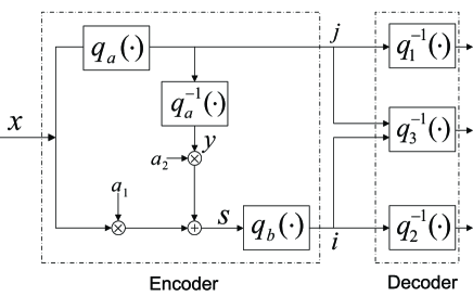
Figure 12: Coding scheme using successive quantization in terms of quantization encoder and decoder.

The successive quantization coding scheme in Fig. 8 is redrawn in terms of quantization encoder and decoder in Fig. 12. The scaling factors $\alpha_{1}$, $\alpha_{2}$, $\beta_{1}$ and $\beta_{2}$ are absorbed into the lossy decoders. The lossless encoder $\gamma$, though important, is not essential in this interpretation and is thus omitted in Fig. 12. The lossy decoders in the receiver are mappings $q_{1}^{-1}:\mathcal{I}_{1}\rightarrow\mathcal{R^{\prime}}_{1}$, $q_{2}^{-1}:\mathcal{I}_{2}\rightarrow\mathcal{R^{\prime}}_{2}$, and $q_{3}^{-1}:\mathcal{I}_{1}\times\mathcal{I}_{2}\rightarrow\mathcal{R^{\prime}}_{3}$, respectively; notice that the corresponding lossy encoders do not necessarily exist in the system.

For simplicity, we assume the lossy encoder $q_{a}$ and $q_{b}$ generate uniform partitions of $\mathcal{R}$, respectively, while the lossy decoder $q_{a}^{-1}$ takes the center points of the partition cells of $q_{a}$ as the reproduction codebook. Notice that function $y=q_{a}(q_{a}^{-1}(x))$ is piecewise constant. A linear combination of $x$ and $y$ is then formed as $s=a_{1}x+a_{2}y$, which is then mapped by the lossy encoder $q_{b}$ to an quantization index $q_{b}(s)$. The task is to find the partition formed by these operations, and it can be done by considering a partition cell $i$, given by $(s_{i},s_{i+1}]$, in the lossy encoder $q_{b}$.

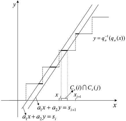
Figure 13: The geometric interpretation of the partitions using successive quantization.

In Fig. 13, this partition cell is represented on the $(x,y)$ plane. For operating points on the dominant face of the SEGC region, it is always true that $\sigma_{T_{0}}^{2}\leq\sigma_{T_{1}}\sigma_{T_{2}}$, which implies $a_{2}\leq 0$ [from (19)], and thus the slope of the line $a_{1}x+a_{2}y=s_{i}$ is always positive. It is clear that, given $q_{b}(s)=i$, $x$ can fall only into the several segments highlighted by the thicker lines in Fig. 13, i.e., into the set $C_{s}(i)=\{x:a_{1}x+a_{2}q_{a}(q_{a}^{-1}(x))\in(s_{i},s_{i+1}]\}$. The information regarding $x$ is thus revealed to the lossy decoder $q_{2}^{-1}$. In the lossy encoder $q_{a}$, the information is revealed to the lossy decoder $q_{1}^{-1}$ in the traditional manner that, when index $j$ is specified, $x$ is in the $j$-th cell, which is $(x_{j},x_{j+1}]$; denote it as $C_{x}(j)=(x_{j},x_{j+1}]$. Jointly, the lossy decoder $q_{3}^{-1}$ has the information that $x$ is in the intersection of the two sets as $C_{s}(i)\cap C_{x}(j)$.

Now we briefly discuss the extension of this interpretation to the case of quantization splitting. The coding scheme in Fig. 9 is redrawn in Fig. 14. Some of the operations in Fig. 9 are absorbed into the lossy decoders. It can be observed that $q_{a}$, $q_{a}^{-1}$ and $q_{b}$ play roles similar to those in Fig. 12; thus, the geometric interpretation for successive quantization can still be utilized. Let $s=b_{1}^{*}x+b_{2}^{*}q_{a}^{-1}(q_{a}(x))$ and define $C_{s}(j)=\{x:b_{1}^{*}x+b_{2}^{*}q_{a}^{-1}(q_{a}(x))\in(s_{j},s_{j+1}]\}$, where $(s_{j},s_{j+1}]$ is the $j$-th partition cell in the lossy encoder $q_{b}$. The variable $s$ is defined differently from that in successive quantization, but this slight abuse of the notation does not cause any ambiguity.

Notice the index $i=(i_{a},i_{c})$ has two components, one is the output of $q_{a}$, and the other is that of $q_{c}$. In a sense, $q_{a}$ and $q_{c}$ are formed in a refinement manner. Thus, the lossy encoder $q_{c}$ and the lossy decoders $q_{2}^{-1}$ and $q_{3}^{-1}$ always have the exact output from $q_{a}$, which in effect confines the source to a finite range. Thus, we need to consider only the case for a fixed $q_{a}(x)$ value. It is obvious that when $q_{a}(x)=i_{0}$ is fixed, $q_{a}^{-1}(i_{0})=y_{i_{0}}$. Consider the linear combination of $r=b_{3}^{*}x+b_{4}^{*}t+b_{5}^{*}q_{a}^{-1}(q_{a}(x))$, where $t=q_{b}^{-1}(q_{b}(s))$. It is similar to the linear combination of $s=b_{1}^{*}x+b_{2}^{*}y$, but with the additional constant term $b_{5}^{*}y_{i_{0}}$, when $i_{0}$ is given. It can be shown that this constant term in fact removes the conditional mean such that $E(r|q_{a}(x)=i_{0})\approx 0$, and the lossy encoder $q_{c}$ is merely a partition of an interval near zero. Thus with $q_{a}(x)=i_{0}$ given, $q_{b}$, $q_{b}^{-1}$ and $q_{c}$ essentially adopt the same roles as $q_{a}$, $q_{a}^{-1}$ and $q_{b}$, respectively, in Fig. 12. This implies a similar geometric interpretation again holds for the additional components in Fig. 14, since $b_{4}^{*}=b_{8}\leq 0$ and $b_{3}^{*}=b_{7}-b_{5}b_{8}>0$. Define $C_{xr}(i_{a},i_{c})=\{x:x\in(x_{i_{a}},x_{i_{a}+1}],r\in(r_{i_{c}},r_{i_{c}+1}]\}$, where $(x_{i_{a}},x_{i_{a}+1}]$ is the $i_{a}$-th partition cell in the lossy encoder $q_{a}$ and $(r_{i_{c}},r_{i_{c}+1}]$ is the $i_{c}$-th partition cell in the lossy encoder $q_{c}$. Given the index pair $(i,j)=(i_{a},i_{c},j)$, the joint lossy decoder $q_{3}^{-1}$ is provided with information that $x\in C_{s}(j)\cap C_{xr}(i_{a},i_{c})$.

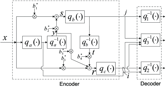
Figure 14: Coding scheme using quantization splitting in terms of quantization encoder and decoder.

VI-B High-Resolution Analysis of Several Special Cases

Below, the high-resolution performance of the proposed coding scheme using scalar quantization is analyzed under several special conditions. Of particular interest is the balanced case, where $R_{1}=R_{2}=R$ and two side distortions are equal, $D_{1}=D_{2}$; significant research effort has been devoted to this case. In the analysis that follows, simplicity is often given priority over rigor; this corresponds to the motivation to introduce this section, which is to provide an intuitive interpretation of the coding schemes.

For the balanced case, it can be shown [21] that at high-resolution if the side distortion is of the form $D_{1}=b\sigma_{x}^{2}2^{-2(1-\eta)R}$, where $0\leq\eta<1$ and $b\geq 1$, the central distortion of an MD system can asymptotically achieve

$$D_{3}\geq\left\{\begin{array}[]{lr}\textstyle{\sigma_{x}^{2}2^{-2R}/2(b+\sqrt{b^{2}-1})}&\eta=0;\\ \textstyle{\sigma_{x}^{2}2^{-2R(1+\eta)}/4b}&0<\eta<1.\\ \end{array}\right.$$ (52)

Notice the condition $0<\eta<1$ in fact corresponds to the condition that $\sigma_{x}^{2}\gg{D_{1}}$ and $D_{1}\gg{D_{3}}$ at high rate. In this case, the central and side distortion product remains bounded by a constant at fixed rate, which is $D_{3}D_{1}\geq\frac{\sigma_{x}^{4}2^{-4R}}{4}$, independent of the tradeoff between them. This product has been used as the information theoretical bound to measure the efficiency of quantization methods [22, 27, 62, 19, 20, 30]. For the sake of simplicity, we focus on the zero-mean Gaussian source, however, because of the tightness of the Shannon lower bound at high-resolution [11], the results of the analysis are applicable with minor changes for other continuous sources with smooth probability density function.

VI-B1 High-resolution analysis for successive quantization

Consider using the quantization method depicted in Fig. 12 to construct two descriptions, such that $D_{1}=D_{2}$, though the rates of the two descriptions are not necessarily equal. For the case $\sigma_{x}^{2}\gg{D_{1}}$ and $D_{1}\gg{D_{3}}$ at high rate, it is clear that $\sigma_{x}^{2}\gg\sigma_{T_{1}}^{2}=\sigma_{T_{2}}^{2}\gg\sigma_{T_{0}}^{2}$. Thus $a_{1}\approx 2$ and $a_{2}\approx-1$ [from (19)], which suggests that the slope of the line $a_{1}x+a_{2}y=s_{i}$ should be approximately $2$ in this case.

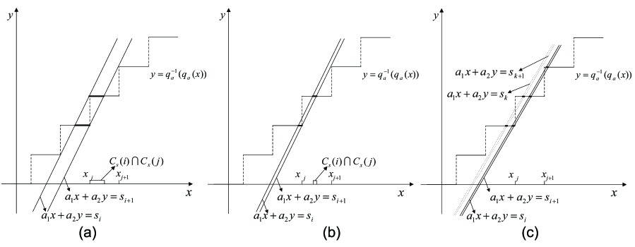
Figure 15: Several special cases of the partition formed using successive quantization. (a) $a_{1}=2$, $a_{2}=-1$, and the stepsize of $q_{a}$ is the same as that of $q_{b}$. (b) $a_{1}=2$, $a_{2}=-1$, but the stepsize of $q_{a}$ is much larger than that of $q_{b}$. (c) When the stepsize of $q_{a}$ is much larger than that of $q_{b}$, by slightly varying $a_{1}$ and $a_{2}$, the two side distortions can be made equal.

Next we consider the three cases depicted in Fig. 15. In Fig. 15 (a), $a_{1}=2$, $a_{2}=-1$ are chosen. By properly choosing the thresholds and the stepsize, a symmetric (between the two descriptions) partition can be formed. In this partition, cells $C_{x}(\cdot)$ and cells $C_{s}(\cdot)$ both are intervals. Furthermore, they form two uniform scalar quantizers with their bins staggered by half the stepsize. This in effect gives the staggered index assignment of [63, 22]. By using this partition, the central distortion is reduced to $1/4$ of the side distortions. Notice that in this case the condition $D_{1}\gg{D_{3}}$ does not hold, but choosing $a_{1}=2$, $a_{2}=-1$ indeed generates two balanced descriptions; this suggests that certain discrepancy occurs when applying the information theoretic results directly to the scalar quantization case. The high-resolution performance of the partition in Fig. 15 (a) is straightforward, being given by $D_{1}=D_{2}\approx\frac{1}{12}\Delta_{a}^{2}\approx\frac{2\pi e}{12}2^{-2R_{1}}\sigma_{x}^{2}$, where the second equality is true when entropy coding is assumed, and $D_{3}\approx\frac{1}{4}D_{1}$ (also see [62]).

In Fig. 15 (b), the stepsize in $q_{b}$, which is denoted by $\Delta_{b}$, is chosen to be much smaller than that of $q_{a}$, which is denoted as $\Delta_{a}$; however, $a_{1}=2$ and $a_{2}=-1$ are kept unchanged. In this case, the partition by $q_{a}$ is still uniform, and the performance of $q_{1}^{-1}$ is given by $D_{1}\approx\frac{1}{12}\Delta_{a}^{2}\approx\frac{2\pi e}{12}2^{-2R_{1}}\sigma_{x}^{2}$. This differs from the previous case in that most of the cells $C_{s}(i)$ are no longer intervals, but rather the union of two non-contiguous intervals, when $\Delta_{a}\gg\Delta_{b}$; for a small portion of the $C_{s}$ cells, each of them can consist of three non-contiguous intervals, but when $\Delta_{a}\gg\Delta_{b}$, this portion is negligible and will be omitted in the discussion which follows. Furthermore, cell $C_{s}(i)$ approximately consists of two length $\Delta_{b}/2$ intervals whose midpoints are $\frac{1}{2}\Delta_{a}$ apart. The distortion achieved by using this partition in the lossy decoder $q_{2}$ is

$$D_{2}\approx(\frac{1}{4}\Delta_{a})^{2}=\frac{3}{4}D_{1}$$ (53)

Intuitively, this says that the average distance of the points in the cell $C_{s}(i)$ from its reproduction codeword is approximately $\frac{1}{4}\Delta_{a}$, which is obviously true given the geometric structure of the cell $C_{s}(i)$. Note that $D_{1}$ and $D_{2}$ are not of equal value.

The rate of the second description is less straightforward, but consider the joint partition revealed to $q_{3}^{-1}$. This partition is almost uniform, while the rate of the output of $q_{b}$ after entropy coding is one bit less than that when the same partition is used in a classical quantizer, because each cell $C_{s}(i)$ consists of two local intervals instead of one as in the classical quantizer. Thus,

$$D_{3}\approx\frac{1}{12}\Delta_{b}^{2}\approx\frac{2\pi e}{12}2^{-2(R_{2}+1)}\sigma_{x}^{2}=\frac{2\pi e}{48}2^{-2R_{2}}\sigma_{x}^{2}$$ (54)

It follows that an achievable high-resolution operating point using scalar quantization is given by $(R_{1},R_{2},D_{1},D_{2},D_{3})$, where $D_{1}=\frac{2\pi e}{12}2^{-2R_{1}}\sigma_{x}^{2}$, $D_{2}=\frac{3}{4}D_{1}$, $D_{3}=\frac{2\pi e}{48}2^{-2R_{2}}\sigma_{x}^{2}$; by symmetry, the operating point $(R_{2},R_{1},D_{2},D_{1},D_{3})$ is also achievable. By time-sharing, an achievable balanced point is $(\frac{R_{1}+R_{2}}{2},\frac{R_{1}+R_{2}}{2},\frac{7}{8}D_{1},\frac{7}{8}D_{1},D_{3})$. Obviously the central and side distortion product is $\frac{7}{8}(\frac{2\pi e}{12})^{2}2^{-2(R_{1}+R_{2})}\sigma_{x}^{2}$, which is only $2.5$ dB away from the information theoretic distortion product. However, time-sharing is not strictly scalar quantization, and later we discuss a method to avoid the time-sharing argument.

In order to make $D_{1}=D_{2}$ when $\Delta_{a}\gg\Delta_{b}$, the values of $a_{2}$ can be varied slightly. First, let $\Delta_{a}$ be fixed such that $D_{1}(\approx\frac{1}{12}\Delta_{a}^{2}\approx\frac{2\pi e}{12}2^{-2R_{1}}\sigma_{x}^{2})$ and $R_{1}$ are then both fixed. It is clear with stepsize $\Delta_{b}$ fixed, as $a_{2}$ decreases from $-1$, the distortion $D_{2}$ increases. A simple calculation shows that when $a_{2}=-4/3$, $D_{2}>D_{1}$; thus, the desired value of $a_{2}$ is in $(-4/3,-1)$, and we find this value to be $a_{2}=-1.0445$. The detailed calculation is relegated to Appendix IV, where the computation of the distortions and rates of this particular quantizer also is given. By using such a value, it can be shown that an achievable high-resolution operating point is $(R_{1},R_{2},D_{1},D_{2},D_{3})$, where $D_{1}=D_{2}\approx\frac{2\pi e}{12}2^{-2R_{1}}\sigma_{x}^{2}$ and $D_{3}\approx 0.8974\cdot\frac{2\pi e}{48}2^{-2R_{2}}\sigma_{x}^{2}$. The rates $R_{1}$ and $R_{2}$ usually are not equal, but the results derived here will be used to construct two balanced descriptions next.

VI-B2 Balanced descriptions using quantization splitting

As previously pointed out, in the quantization splitting coding scheme $\sigma_{T_{3}}^{2}$ should be chosen to be $2\sigma_{T_{0}}\sigma_{T_{1}}$ when balanced descriptions are required; then $\sigma_{T_{1}}\gg\sigma_{T_{0}}$ implies $\sigma_{T_{1}}^{2}\gg\sigma_{T_{3}}^{2}\gg\sigma_{T_{0}}^{2}$. It follows that $b_{1}^{*}\approx 2$, $b_{2}^{*}=-1$, $b_{3}^{*}\approx 2$, $b_{4}^{*}\approx-1$ and $b_{5}^{*}\approx 3$. We make the following remarks assuming these values.

• The conditional expectation $E(r|q_{a}(x)=i)$ is approximately zero, which implies only the case in which $q_{a}^{-1}((q(x)))=0$ needs to be considered. This is obvious from the geometric structure given in Fig. 15 (b) and the values of $b^{*}$s.

• The partition formed by $q_{c}$ does not improve the distortion $D_{1}$ over $q_{a}$. This is because the slope of the line $b_{3}^{*}x+b_{4}^{*}t+b_{5}^{*}y_{i_{0}}=r_{i}$ on the $(x,t)$ plane is given in such a way that it almost aligns with the function $t=f(x)$. In such a case, the cell $C_{xr}(i_{a},i_{b})$ consists of segments from almost every cell $C_{s}(j)$ for which $C_{s}(j)\cap\{x:q_{a}(x)=i_{a}\}\neq\emptyset$. Intuitively, it is similar to letting the slope of $a_{1}x+a_{2}y=s_{i}$ have a slope of $1$ in Fig. 15 (b), such that the distortion $D_{2}$ does not improve much over $\sigma_{x}^{2}$ in the successive quantization case.

With these two remarks, consider constructing balanced descriptions using scalar quantization for $R_{1}=R_{2}$ as follows. Chose $b_{1}^{*}=2$ and $b_{2}^{*}=-1.0445$ such that, without the lossy encoder $q_{c}$, the distortions $D_{1}$ and $D_{2}$ are made equal. Denote the entropy rate of $q_{a}$ as $R_{1a}$ and that of $q_{b}$ as $R_{2}$. Let $b_{3}^{*}=2$, $b_{4}^{*}=-1$ but $b_{5}^{*}=2.9555$ such that $E(r|q_{a}(x)=i)$ is approximately zero. By doing this, $b_{3}^{*}x+b_{4}^{*}t+b_{5}^{*}y_{i_{0}}=r_{i}$ on the $(x,t)$-plane aligns with the function $t=f(x)$, and thus the remaining rate $R_{1}-R_{1a}$ is used by $q_{c}$ to improve $D_{3}$, but $D_{1}$ and $D_{2}$ are not further improved. Since $q_{a}$ and $q_{b}$ are both operating on high resolution, assuming $R_{1}-R_{1a}$ is also high, then $q_{c}$ partitions each $x\in C_{s}(j)\cap C_{xr}(i_{a},i_{c})$ into $2^{R_{1}-R_{1a}}$ uniform segments, thus improve $D_{0}$ by a factor of $2^{-2(R_{1}-R_{1a})}$.

Using this construction, we can achieve a balanced high-resolution operating point of $(R_{1},R_{1},D_{1},D_{1},D_{0})$ without time-sharing, where $D_{1}=\frac{2\pi e}{12}2^{-2R_{1a}}\sigma_{x}^{2}$ and $D_{0}\approx 0.8974\cdot\frac{2\pi e\sigma_{x}^{2}}{48}2^{-2(2R_{1}-R_{1a})}$. Thus, when $\sigma_{x}^{2}\gg D_{1}=D_{2}\gg D_{3}$, the central and side distortion product is $2.596$ dB away from the information theoretic distortion product. This is a better upper bound than the best known upper bound of the granular distortion using scalar quantization, which is $2.67$ dB away from the information theoretic distortion product [22]; this previous bound was derived in [22] using the multiple description scalar quantization scheme proposed by Vaishampayan [19, 20] with systematic optimization of quantization thresholds. It should be pointed out that the results regarding the granular distortion also apply to other continuous source as in the approach taken in [22]. Thus for any sources with smooth pdf, this granular distortion can be $2.596$ away from the Shannon outer bound which is tight at high resolution.

VI-C Optimization of Scalar Quantization Scheme

The analysis in the previous subsection reveals that for the scalar case the proposed coding scheme can potentially achieve better performance than the previous techniques based on scalar quantization [19, 20, 22]. However, for the proposed coding scheme to perform competitively at low rate with scalar quantization, better methods to optimize the quantizer should be used. Specifically, the following improvements are immediate:

• Given the partition formed by the lossy encoders, the lossy decoder $q_{1}^{-1}$, $q_{2}^{-1}$ and $q_{3}^{-1}$ should optimize the reproduction codebook to be the conditional mean of the codecells.

• The index $i_{a}$ and $i_{b}$ should be jointly entropy-coded instead of being separately coded, and such a joint codebook should be designed.

• The lossy encoder $q_{c}$ can be designed for each output index of $q_{a}$, and thus operates adaptively.

• The encoder partition should be better optimized; the design method for multi-stage vector quantization offers a possible approach [64].

These improvements currently are under investigation; a systematic comparison of these improvements is beyond the scope of this article and thus will not be included.

VII Conclusion

We proposed a lattice quantization scheme which can achieve the whole Gaussian MD rate-distortion region. Our scheme is universal in the sense that it only needs the information of the first and second order statistics of the source. Our scheme is optimal for Gaussian sources at any resolution and asymptotically optimal for all smooth sources at high resolution.

Our results, along with a recent work by Erez and Zamir [65], consolidate the link between MMSE estimation and lattice coding (/quantization), or in a more general sense, the connection between Wiener and Shannon theories as illuminated by Forney [66, 67].

Although the linear MMSE structure is optimal in achieving the Gaussian MD rate-distortion region as the dimension of the (optimal) lattice quantizers goes to infinity, it is not optimal for finite dimensional lattice quantizers since the distribution of quantization errors is no longer Gaussian. Using nonlinear structure to exploit the higher order statistics may result in better performance.

We also want to point out that our derivation does not rely on the fact that the source is i.i.d. in time. The proposed MD quantization system is directly applicable for a general stationary source, although it may be more desirable to whiten the process first.

Appendix A Gram-Schmidt Orthogonalization for Random Vectors

Let $\mathcal{H}_{v}$ denote the set of all $n$-dimensional, finite-covariance-matrix, zero-mean, real random (column) vectors. $\mathcal{H}_{v}$ becomes a Hilbert space under the inner product mapping

$$\langle\mathbf{X},\mathbf{Y}\rangle=\mathbb{E}(\mathbf{X}\mathbf{Y}^{T}):\mathcal{H}_{v}\times\mathcal{H}_{v}\rightarrow\mathcal{R}^{n\times n}.$$

For $\mathbf{X}^{M}_{1}=(\mathbf{X}_{1},\mathbf{X}_{2},\cdots,\mathbf{X}_{M})^{T}$ with $\mathbf{X}_{i}\in\mathcal{H}_{v}$, $i=1,\cdots,M$, the Gram-Schmidt orthogonalization proceeds as follows:

$$\mathbf{B}_{1} = \mathbf{X}_{1},$$

$$\mathbf{B}_{i} = \mathbf{X}_{i}-\sum\limits_{j=1}^{i-1}\frac{\mathbb{E}(\mathbf{X}_{i}\mathbf{B}_{j}^{T})}{\mathbb{E}(\mathbf{B}_{j}\mathbf{B}_{j}^{T})}\mathbf{B}_{j},\quad i=2,\cdots,M.$$

Note: $\frac{\mathbb{E}(\mathbf{X}_{i}\mathbf{B}_{j}^{T})}{\mathbb{E}(\mathbf{B}_{j}\mathbf{B}_{j}^{T})}$ can be any matrix in $\mathcal{R}^{n\times n}$ if $\mathbf{B}_{j}=\mathbf{0}$.

We can also write

$$\mathbf{B}_{1} = \mathbf{X}_{1},$$

$$\mathbf{B}_{i} = \mathbf{X}_{i}-\widetilde{K}_{i-1}\mathbf{X}^{i-1}_{1},\quad i=2,\cdots,M,$$

where $\widetilde{K}_{i-1}\in\mathcal{R}^{n\times(i-1)n}$ is a matrix satisfying $\widetilde{K}_{i-1}K_{\mathbf{X}^{i-1}_{1}}=K_{\mathbf{X}_{i}\mathbf{X}^{i-1}_{1}}$. When $K_{\mathbf{X}^{i-1}_{1}}$ is invertible, we have $\widetilde{K}_{i-1}=K_{\mathbf{X}_{i}\mathbf{X}^{i-1}_{1}}K^{-1}_{\mathbf{X}^{i-1}_{1}}$. Here $K_{\mathbf{X}^{i-1}_{1}}$ is the covariance matrix of $(\mathbf{X}_{1},\cdots,\mathbf{X}_{i})^{T}$ and $K_{\mathbf{X}_{i}\mathbf{X}_{1}^{i-1}}=\mathbb{E}[\mathbf{X}_{i}(\mathbf{X}_{1},\cdots,\mathbf{X}_{i-1})^{T}]$.

Again, a sequential quantization system can be constructed with $\mathbf{X}_{1}$ as the input to generate a zero-mean random vector $\mathbf{\widetilde{X}}^{M}_{1}=(\mathbf{\widetilde{X}}_{1},\cdots,\mathbf{\widetilde{X}}_{M})^{T}$ whose covariance matrix is also $K_{\mathbf{X}^{M}_{1}}$. Assume $K_{\textbf{B}_{i}}=\mathbb{E}\mathbf{B}_{i}\mathbf{B}_{i}^{T}$ is nonsingular for $i=2,\cdots,M$. Let $Q_{i,n}(\cdot)$ be an $n$-dimensional lattice quantizer, $i=1,2,\cdots,L-1$. The dither $\mathbf{Z}_{i}$ is an $n$-dimensional random vector, uniformly distributed over the basic cell of $Q_{i,n}$, $i=1,2,\cdots,M-1$. Suppose $(\mathbf{X}_{1},\mathbf{Z}_{1},\cdots,\mathbf{Z}_{M-1})$ are independent, and $\mathbb{E}\mathbf{Z}_{i}\mathbf{Z}_{i}^{T}=K_{\mathbf{B}_{i}}$, $i=1,2,\cdots,M$. Define

$$\mathbf{\widetilde{X}}_{1} = \mathbf{X}_{1},$$ (55)

$$\mathbf{\widetilde{X}}_{i} = Q_{i-1,n}\left(\widetilde{K}_{i-1}\mathbf{\widetilde{X}}^{i-1}_{1}+\mathbf{Z}_{i-1}\right)-\mathbf{Z}_{i-1},\quad i=2,\cdots,M.$$ (56)

It is easy to show that $\mathbf{X}^{M}_{1}$ and $\mathbf{\widetilde{X}}^{M}_{1}$ have the same covariance matrix.

As in the scalar case, a single quantizer can be reused if pre- and post-filters are incorporated. Specifically, given an $n$-dimensional lattice quantizer $Q_{n}(\cdot)$, let the dither $\mathbf{Z}^{\prime}_{i}$ be an $n$-dimensional random vector, uniformly distributed over the basic cell of $Q_{n}$ with nonsingular covariance matrix $K_{\mathbf{Z}^{\prime}}=\mathbb{E}\textbf{Z}^{\prime}_{i}{\textbf{Z}^{\prime}}^{T}_{i}$. Let $A_{i}$ be an $n\times n$ nonsingular matrix such that $A_{i}K_{\mathbf{Z}^{\prime}}A^{T}_{i}=K_{\mathbf{B}_{i+1}}$, $i=1,2,\cdots,M-1$. Suppose $(\mathbf{X}_{1},\mathbf{Z}^{\prime}_{1},\cdots,\mathbf{Z}^{\prime}_{M-1})$ are independent. Define

$$\mathbf{\overline{X}}_{1} = \mathbf{X}_{1},$$

$$\mathbf{\overline{X}}_{i} = A_{i-1}\left[Q_{n}\left(A^{-1}_{i-1}\widetilde{K}_{i-1}\mathbf{\overline{X}}^{i-1}_{1}+\mathbf{Z}^{\prime}_{i-1}\right)-\mathbf{Z}^{\prime}_{i-1}\right],\quad i=2,\cdots,M.$$

It is easy to verify that $\mathbf{X}^{M}_{1}$ and $\mathbf{\widetilde{X}}^{M}_{1}$ have the same covariance matrix by invoking property 2) of the ECDQ. Here introducing the prefilter $A^{-1}_{i}$ and the postfilter $A_{i}$ is equivalent to shaping $Q(\cdot)$ by $A_{i}$, which induces a new quantizer $Q_{i,n}(\cdot)$ given by $Q_{i,n}(\mathbf{x})=A_{i}Q_{n}(A^{-1}_{i}\mathbf{}x)$.

Suppose $K_{\mathbf{B}_{i}}$ is singular for some $i$, say $K_{\mathbf{B}_{i}}$ is of rank $k$ with $k<n$. For this type of degenerate case, the quantization operation should be carried out in the nonsingular subspace of $K_{\mathbf{B}_{i}}$. Let $K_{\mathbf{B}_{i}}=U\Lambda U^{T}$ be the eigenvalue decomposition of $K_{\mathbf{B}_{i}}$. Without loss of generality, assume $\Lambda=\mbox{diag}\{\lambda_{1},\cdots,\lambda_{k},0,\cdots,0\}$, where $\lambda_{i}>0$ for all $i=1,2,\cdots,k$. Define $\Lambda_{k}=\mbox{diag}\{\lambda_{1},\cdots,\lambda_{k}\}$. Now replace the $n$-dimensional quantizer $Q_{i-1,n}(\cdot)$ in (56) by a $k$-dimensional quantizer $Q_{i-1,k}(\cdot)$ and replace the dither $\mathbf{Z}_{i-1}$ by a dither $\mathbf{\widetilde{Z}}_{i-1}$ which is a $k$-dimensional random vector, uniformly distributed over the basic cell of $Q_{i-1,k}$ with $\mathbb{E}\mathbf{\widetilde{Z}}_{i-1}\mathbf{\widetilde{Z}}_{i-1}^{T}=\Lambda_{k}$. Let

$$\left[\mathbf{\widetilde{X}}_{i}\right]_{1,k}=Q_{i-1,k}\left(\left[U^{T}\widetilde{K}_{i-1}\mathbf{\widetilde{X}}^{i-1}_{1}\right]_{1,k}+\mathbf{\widetilde{Z}}_{i-1}\right)-\mathbf{\widetilde{Z}}_{i-1}$$

and we have

$$\mathbf{\widetilde{X}}_{i}=U\begin{pmatrix}\left[\mathbf{\widetilde{X}}_{i}\right]_{1,k}\\ \left[U^{T}\widetilde{K}_{i-1}\mathbf{\widetilde{X}}^{i-1}_{1}\right]_{k+1,n}\end{pmatrix},$$

where $\left[U^{T}\widetilde{K}_{i-1}\mathbf{\widetilde{X}}^{i-1}_{1}\right]_{1,k}$ is a column vector containing the first $k$ entries of $U^{T}\widetilde{K}_{i-1}\mathbf{\widetilde{X}}^{i-1}_{1}$ and $\left[U^{T}\widetilde{K}_{i-1}\mathbf{\widetilde{X}}^{i-1}_{1}\right]_{k+1,n}$ is a column vector that contains the remaining entries of $U^{T}\widetilde{K}_{i-1}\mathbf{\widetilde{X}}^{i-1}_{1}$.

Appendix B Proof of Theorem V.3

It is easy to verify that as $D_{1},D_{2},D_{3}\rightarrow 0$, we have $\frac{\sigma^{2}_{T_{0}}}{D_{3}}\rightarrow 1$, $\frac{\sigma^{2}_{T_{0}}+\sigma^{2}_{T_{i}}}{D_{3}}\rightarrow 1$, and $\frac{\sigma_{T_{i}}}{\sqrt{D_{i}-D_{3}}}\rightarrow 1$, $i=1,2$. Let $\sigma^{2}_{T_{3}}\in\left[0,M\left(\frac{D_{3}}{D_{1}}(\sqrt{D_{1}-D_{3}}+\sqrt{D_{2}-D_{3}})^{2}+D_{2}\right)\right]$, where $M$ is a fixed large number. Clearly, $\sigma^{2}_{T_{3}}\rightarrow 0$ as $D_{1},D_{2},D_{3}\rightarrow 0$.

For the MD quantization scheme shown in Fig. 9, we have

$$R_{1} = \frac{1}{n}H(Q^{*}_{2,n}(b^{*}_{1}\mathbf{X}+b^{*}_{2}{\mathbf{\widetilde{W}}^{\prime}_{2}}+{\mathbf{Z}^{*}_{2}}^{n})|{\mathbf{Z}^{*}_{2}})$$

$$= \frac{1}{n}h(\mathbf{X}+b^{*}_{2}{\mathbf{N}^{*}_{1}}+{\mathbf{N}^{*}_{2}})-\frac{1}{n}h({\mathbf{N}^{*}_{2}})$$

$$= \frac{1}{n}h(\mathbf{X}+b^{*}_{2}{\mathbf{N}^{*}_{1}}+{\mathbf{N}^{*}_{2}})-\frac{1}{2}\log\frac{\mathbb{E}{\widetilde{B}_{3}}^{2}}{G^{opt}_{n}},$$

$$R_{2} = \frac{1}{n}H(Q^{*}_{1,n}(\mathbf{X}+{\mathbf{Z}^{*}_{1}})|{\mathbf{Z}^{*}_{1}})+\frac{1}{n}H(Q^{*}_{3,n}(b^{*}_{3}\mathbf{X}+b^{*}_{4}\mathbf{\widetilde{W}}_{1}+b^{*}_{5}{\mathbf{\widetilde{W}}^{\prime}_{2}}+{\mathbf{Z}^{*}_{3}})|{\mathbf{Z}^{*}_{3}})$$

$$= \frac{1}{n}h(\mathbf{X}+{\mathbf{N}^{*}_{1}})-\frac{1}{n}h({\mathbf{N}^{*}_{1}})+\frac{1}{n}h(b^{*}_{3}\mathbf{X}+b^{*}_{4}\mathbf{\widetilde{W}}_{1}^{n}+b^{*}_{5}{\mathbf{\widetilde{W}}^{\prime}_{2}}+{\mathbf{N}^{*}_{3}})-\frac{1}{n}h({\mathbf{N}^{*}_{3}})$$

$$\leq \frac{1}{n}h(\mathbf{X}+{\mathbf{N}^{*}_{1}})-\frac{1}{n}h({\mathbf{N}^{*}_{1}})+\frac{1}{n}h(b_{7}{\mathbf{\overline{B}}_{2}}+b_{8}{\mathbf{\overline{B}}_{3}}+{\mathbf{\overline{B}}_{4}})-\frac{1}{n}h({\mathbf{N}^{*}_{3}})$$

$$= \frac{1}{n}h(\mathbf{X}+{\mathbf{N}^{*}_{1}})-\frac{1}{2}\log\frac{\mathbb{E}{\widetilde{B}_{2}}^{2}}{G^{opt}_{n}}+\frac{1}{2}\log\left[2\pi e(b^{2}_{7}\mathbb{E}{\overline{B}^{2}_{2}}+b^{2}_{8}\mathbb{E}{\overline{B}^{2}_{3}}+\mathbb{E}{\overline{B}^{2}_{4}})\right]-\frac{1}{2}\log\frac{\mathbb{E}{\overline{B}^{2}_{4}}}{G^{opt}_{n}}.$$

Since $\frac{1}{n}h(\mathbf{X}+{\mathbf{N}^{*}_{1}})=h(X)+o(1)$ and $\frac{1}{n}h(\mathbf{X}+b^{*}_{2}{\mathbf{N}^{*}_{1}}+{\mathbf{N}^{*}_{2}})=h(X)+o(1)$ as $D_{1},D_{2},D_{3}\rightarrow 0$, it follows that

$$R_{1} = h(X)-\frac{1}{2}\log\frac{\mathbb{E}{\widetilde{B}_{3}}^{2}}{G^{opt}_{n}}+o(1)$$

$$= \frac{1}{2}\log\frac{P_{X}(D_{2}+\sigma^{2}_{T_{3}})}{D_{3}(\sqrt{D_{1}-D_{3}}+\sqrt{D_{2}-D_{3}})^{2}+\sigma^{2}_{T_{3}}D_{1}}+\frac{1}{2}\log(2\pi eG^{opt}_{n})+o(1),$$

$$R_{2} \leq h(X)-\frac{1}{2}\log\frac{\mathbb{E}{\widetilde{B}_{2}}^{2}}{G^{opt}_{n}}+\frac{1}{2}\log\left[2\pi e(b^{2}_{7}\mathbb{E}{\overline{B}^{2}_{2}}+b^{2}_{8}\mathbb{E}{\overline{B}^{2}_{3}}+\mathbb{E}{\overline{B}^{2}_{4}})\right]-\frac{1}{2}\log\frac{\mathbb{E}{\overline{B}_{4}}^{2}}{G^{opt}_{n}}+o(1)$$

$$= \frac{1}{2}\log\frac{P_{X}}{D_{2}+\sigma^{2}_{T_{3}}}+\frac{1}{2}\log\frac{D_{3}(\sqrt{D_{1}-D_{3}}+\sqrt{D_{2}-D_{3}})^{2}+\sigma^{2}_{T_{3}}D_{1}}{D_{3}(\sqrt{D_{1}-D_{3}}+\sqrt{D_{2}-D_{3}})^{2}}+\log(2\pi eG^{opt}_{n})+o(1).$$

So we have

$$R_{1}+R_{2}\leq\frac{1}{2}\log\frac{P^{2}_{X}}{D_{2}(\sqrt{D_{1}-D_{3}}+\sqrt{D_{2}-D_{3}})^{2}}+\frac{3}{2}\log(2\pi eG^{opt}_{n}).$$

When $\sigma^{3}_{T_{3}}=0$, there is no quantization splitting and the quantizer $Q^{*}_{3,n}(\cdot)$ can be removed. In this case, we have

$$R_{1} = \frac{1}{2}\log\frac{P_{X}D_{2}}{D_{3}(\sqrt{D_{1}-D_{3}}+\sqrt{D_{2}-D_{3}})^{2}}+\frac{1}{2}\log(2\pi eG^{opt}_{n})+o(1),$$

$$R_{2} = \frac{1}{2}\log\frac{P_{X}}{D_{2}}+\frac{1}{2}\log(2\pi eG^{opt}_{n})+o(1)$$

When $\sigma^{3}_{T_{3}}=M\left[\frac{D_{3}}{D_{1}}(\sqrt{D_{1}-D_{3}}+\sqrt{D_{2}-D_{3}})^{2}+D_{2}\right]$, we have

$$R_{1} = \frac{1}{2}\log\frac{P_{X}}{D_{1}}+\frac{1}{2}\log(2\pi eG^{*}_{2,n})+\epsilon(M)+o(1),$$

$$R_{2} = \frac{1}{2}\log\frac{P_{X}D_{1}}{D_{3}(\sqrt{D_{1}-D_{3}}+\sqrt{D_{2}-D_{3}})^{2}}+\log(2\pi eG^{opt}_{n})-\epsilon(M)+o(1),$$

where $\epsilon(M)\rightarrow 0$ as $M\rightarrow\infty$. Therefore, the region

$$R_{1} = \frac{1}{2}\log\frac{P_{X}}{D_{1}}+\frac{1}{2}\log(2\pi eG^{opt}_{n})+\epsilon(M)+o(1),$$

$$R_{2} = \frac{1}{2}\log\frac{P_{X}}{D_{2}}+\frac{1}{2}\log(2\pi eG^{opt}_{n})+o(1),$$

$$R_{1}+R_{2} = \frac{1}{2}\log\frac{P^{2}_{X}}{D_{2}(\sqrt{D_{1}-D_{3}}+\sqrt{D_{2}-D_{3}})^{2}}+\frac{3}{2}\log(2\pi eG^{opt}_{n})+o(1)$$

is achievable.

By symmetry, the region

$$R_{1} = \frac{1}{2}\log\frac{P_{X}}{D_{1}}+\frac{1}{2}\log(2\pi eG^{opt}_{n})+o(1),$$

$$R_{2} = \frac{1}{2}\log\frac{P_{X}}{D_{2}}+\frac{1}{2}\log(2\pi eG^{opt}_{n})+\epsilon(M)+o(1),$$

$$R_{1}+R_{2} = \frac{1}{2}\log\frac{P^{2}_{X}}{D_{2}(\sqrt{D_{1}-D_{3}}+\sqrt{D_{2}-D_{3}})^{2}}+\frac{3}{2}\log(2\pi eG^{opt}_{n})+o(1)$$

is achievable via the other form of quantization splitting. The desired result follows by combining these two regions and choosing $M$ large enough.

Appendix C Proof of Theorem V.4

We shall only give a heuristic argument here. The rigorous proof is similar to that of Theorem 3 in [37] and thus is omitted.

It is well-known that the distribution of the quantization noise converges to a white Gaussian distribution in the divergence sense as the dimension of the optimal lattice becomes large [37]. So we can approximate $\mathbf{N}^{*}_{i}$ by $\mathbf{N}^{G}_{i}$, where $\mathbf{N}^{G}_{i}$ is a zero-mean Gaussian vector with the same covariance as that of $\mathbf{N}^{*}_{i}$, $i=1,2,3$. Therefore, for large $n$, we have

$$\frac{1}{n}h(\mathbf{X}+{\mathbf{N}^{*}_{1}})-\frac{1}{n}h({\mathbf{N}^{*}_{1}}) \approx \frac{1}{n}h(\mathbf{X}+{\mathbf{N}^{G}_{1}})-\frac{1}{n}h({\mathbf{N}^{G}_{1}})$$

$$= h\left(X+N^{G}_{1}\right)-h\left(N^{G}_{1}\right),$$

$$h\left(b^{*}_{1}\mathbf{X}+b^{*}_{2}{\mathbf{\widetilde{W}}^{\prime}_{2}}+{\mathbf{N}^{*}_{2}}\right)-\frac{1}{n}h\left({\mathbf{N}^{*}_{2}}\right) = \frac{1}{n}h\left(\mathbf{X}+b^{*}_{2}\mathbf{N}^{*}_{1}+\mathbf{N}^{*}_{2}\right)-\frac{1}{n}h\left(\mathbf{N}^{*}_{2}\right)$$

$$\approx \frac{1}{n}h\left(\mathbf{X}+b^{*}_{2}\mathbf{N}^{G}_{1}+\mathbf{N}^{G}_{2}\right)-\frac{1}{n}h\left(\mathbf{N}^{G}_{2}\right)$$

$$= h\left(X+b^{*}_{2}N^{G}_{1}+N^{G}_{2}\right)-h\left(N^{G}_{2}\right),$$

and

$$\frac{1}{n}h\left(b^{*}_{3}\mathbf{X}+b^{*}_{4}\mathbf{\widetilde{W}}_{1}^{n}+b^{*}_{5}{\mathbf{\widetilde{W}}^{\prime}_{2}}+{\mathbf{N}^{*}_{3}}\right)-\frac{1}{n}h\left({\mathbf{N}^{*}_{3}}\right)$$

$$= \frac{1}{n}h\left((b^{*}_{3}+b^{*}_{1}b^{*}_{4}+b^{*}_{2}b^{*}_{4}+b^{*}_{5})\mathbf{X}+(b^{*}_{2}b^{*}_{4}+b^{*}_{5})\mathbf{N}^{*}_{1}+b^{*}_{4}\mathbf{N}^{*}_{2}+\mathbf{N}^{*}_{3}\right)-\frac{1}{n}h\left(\mathbf{N}^{*}_{3}\right)$$

$$\approx \frac{1}{n}h\left((b^{*}_{3}+b^{*}_{1}b^{*}_{4}+b^{*}_{2}b^{*}_{4}+b^{*}_{5})\mathbf{X}+(b^{*}_{2}b^{*}_{4}+b^{*}_{5})\mathbf{N}^{G}_{1}+b^{*}_{4}\mathbf{N}^{G}_{2}+\mathbf{N}^{G}_{3}\right)-\frac{1}{n}h\left(\mathbf{N}^{G}_{3}\right)$$

$$= h\left((b^{*}_{3}+b^{*}_{1}b^{*}_{4}+b^{*}_{2}b^{*}_{4}+b^{*}_{5})X+(b^{*}_{2}b^{*}_{4}+b^{*}_{5})N^{G}_{1}+b^{*}_{4}N^{G}_{2}+N^{G}_{3}\right)-h\left(N^{G}_{3}\right).$$

Appendix D The calculation of scalar operating point using successive quantization

Observe in Fig. 15 (c) that the value $a_{2}$ is slightly different from $-1$, such that a portion of the $C_{s}$ cells consist of three length $\frac{1}{2}\Delta_{b}$ intervals which are approximately $\frac{-a_{2}}{2}\Delta_{a}$ apart (denote the set of this first class of cells as $C_{s}^{\prime}$), while the other $C_{s}$ cells consist of only two length $\frac{1}{2}\Delta_{b}$ which are also $\frac{-a_{2}}{2}\Delta_{a}$ apart (denote the set of this second class of cells as $C_{s}^{\prime\prime}$); the ratio between the cardinalities of these two sets is function of $a_{2}$, which is approximately $\frac{-3-3a_{2}}{4+3a_{2}}$. Here we again ignore the cells $C_{s}$ whose constituent segments are at the border of $q_{a}$ partition cells, which is a negligible portion when $\Delta_{a}\gg\Delta_{b}$. The average distortion for each first class cell $C_{s}$ is approximately $\frac{2}{3}(\frac{-a_{2}}{2}\Delta_{a})^{2}$, while the average distortion for each second class cell $C_{s}$ is approximately $(\frac{1}{2}\cdot\frac{-a_{2}}{2}\Delta_{a})^{2}$. Thus, the distortion $D_{2}$ can be approximated as

$$D_{2} \approx (-3-3a_{2})\cdot\frac{2}{3}(\frac{-a_{2}}{2}\Delta_{a})^{2}+(4+3a_{2})(\frac{1}{2}\frac{-a_{2}}{2}\Delta_{a})^{2}$$ (57)

$$= \frac{-1}{16}(5a_{2}+4)a_{2}^{2}{\Delta_{a}}^{2}$$

Notice that $-3-3a_{2}+4+3a_{2}=1$; thus, $(-3-3a_{2})$ is the percentage of the first class cells in all the $C_{s}$ cells. Letting $D_{1}=D_{2}=\frac{1}{12}{\Delta_{a}}^{2}$, we can solve for $a_{2}$; the only real solution to this equation is $a_{2}=-1.0445$. The distortion $D_{3}$ is approximately $\frac{1}{12}(\frac{1}{2}\Delta_{b})^{2}$, by using an almost uniform partition of stepsize $\frac{1}{2}\Delta_{b}$. To approximate the entropy rate for $q_{b}$, consider the rate contribution from the first class $C_{s}$ cells, namely

$$R_{2}^{\prime} = -\sum_{C_{s}(i)\in C_{s}^{\prime}}p(q_{2}^{-1}(i))\frac{3}{2}\Delta_{b}\log_{2}(p(q_{2}^{-1}(i))\frac{3}{2}\Delta_{b})$$ (58)

$$\approx (3+3a_{2})\log_{2}(\frac{3}{2}\Delta_{b})-\sum_{C_{s}(i)\in C_{s}^{\prime}}p(q_{2}^{-1}(i))\frac{3}{2}\Delta_{b}\log_{2}(p(q_{2}^{-1}(i)))$$

where $p(x)$ is the pdf of the source, and the second approximation comes from taking the percentage of the first class cells in all the $C_{s}$ cells as the probability that a random $C_{s}$ is a first class cell. Similarly the rate contribution from the second class $C_{s}$ cells is

$$R_{2}^{\prime\prime} = -\sum_{C_{s}(i)\in C_{s}^{\prime\prime}}p(q_{2}^{-1}(i))\frac{2}{2}\Delta_{b}\log_{2}(p(q_{2}^{-1}(i))\frac{2}{2}\Delta_{b})$$ (59)

$$\approx -(4+3a_{2})\log_{2}(\frac{2}{2}\Delta_{b})-\sum_{C_{s}(i)\in C_{s}^{\prime\prime}}p(q_{2}^{-1}(i))\frac{2}{2}\Delta_{b}\log_{2}(p(q_{2}^{-1}(i)))$$

Thus, the rate $R_{2}$ can be approximated as

$$R_{2} \approx R_{2}^{\prime}+R_{2}^{\prime\prime}$$ (60)

$$\approx -\log_{2}(\Delta_{b})+(3+3a_{2})\log_{2}(\frac{3}{2})-\sum_{C_{s}(i)\in C_{s}^{\prime}}p(q_{2}^{-1}(i))\frac{3}{2}\Delta_{b}\log_{2}(p(q_{2}^{-1}(i)))$$

$$-\sum_{C_{s}(i)\in C_{s}^{\prime\prime}}p(q_{2}^{-1}(i))\frac{2}{2}\Delta_{b}\log_{2}(p(q_{2}^{-1}(i))).$$

When $q_{a}(\cdot)$ is high resolution, $p(q_{2}^{-1}(i))$ is approximately equal to $p(x)$, for any $x\in C_{s}(i)$, and thus equal to $p(q_{3}^{-1}(i,\cdot))$. Using this approximation and taking $\frac{1}{2}\Delta_{b}$ as $\delta x$, the last two terms in (60) can be approximated by an integral, which is in fact $h(p)$, the differential entropy of the source. It follows that

$$R_{2} \approx R_{2}^{\prime}+R_{2}^{\prime\prime}$$ (61)

$$\approx -\log_{2}(\Delta_{b})+(3+3a_{2})\log_{2}(\frac{3}{2})+h(p)$$

where $h(p)=\frac{1}{2}\log(2\pi e\sigma_{x}^{2})$ for the Gaussian source. Thus, $D_{3}\approx\frac{1}{12}(\frac{1}{2}\Delta_{b})^{2}\approx 0.8974\cdot\frac{2\pi e\sigma_{x}^{2}}{48}2^{-2R_{2}}$.

References

- [1] H. Witsenhausen, “On source networks with minimal breakdown degradation,” Bell Syst. Tech. J., vol. 59, no. 6, pp. 1083-1087, July-Aug. 1980.
- [2] J. Wolf, A.Wyner and J. Ziv, “Source coding for multiple descriptions,” Bell Syst. Tech. J., vol. 59, no. 8, pp. 1417-1426, Oct. 1980.
- [3] L. Ozarow, “On a source coding problem with two channels and three receivers,” Bell Syst. Tech. J., vol. 59, no. 10, pp. 1909-1921, Dec. 1980.
- [4] H. S. Witsenhausen and A. D. Wyner, “Source coding for multiple descriptions, II: A binary source,” Bell Syst. Tech. J., vol. 60, pp. 2281-2292, Dec. 1981.
- [5] A. A. El Gamal and T. M. Cover, “Achievable rates for multiple descriptions,” IEEE Trans. on Inform. Theory, vol.IT-28, pp. 851-857, Nov. 1982.
- [6] R. Ahlswede, “The rate-distortion region for multiple descriptions without excess rate,” IEEE Trans. on Inform. Theory, vol. IT-31, pp. 721-726, Nov. 1985.
- [7] Z. Zhang and T. Berger, “New results in binary multiple descriptions,” IEEE Trans. on Inform. Theory, vol. IT-33, pp. 502-521, July 1987.
- [8] H. S.Witsenhausen and A. D.Wyner, “On team guessing with independent information,” Math. Oper. Res., vol. 6, pp. 293-304, May 1981.
- [9] T. Berger and Z. Zhang, “Minimum breakdown degradation in binary source coding,” IEEE Trans. Inform. Theory, vol. IT-29, pp. 807-814, Nov. 1983.
- [10] R. Ahlswede, “On multiple descriptions and team guessing,” IEEE Trans. Inform. Theory, vol. IT-32, pp. 543-549, July 1986.
- [11] R. Zamir, “Gaussian codes and Shannon bounds for multiple descriptions,” IEEE Trans. Inform. Theory, vol. 45, pp. 2629-2635, Nov. 1999.
- [12] F. W. Fu, R. W. Yeung, and R. Zamir, “On the rate-distortion region for multiple descriptions,” IEEE Trans. Inform. Theory, vol. 48, pp. 2012-2021, July 2002.
- [13] H. Feng and M. Effros, “On the rate loss of multiple description source codes,” IEEE Trans. Info. Theory, vol. 51, pp. 671-683, Feb. 2005.
- [14] L. Lastras-Montao and V. Castelli, “Near sufficiency of random coding for two descriptions,” IEEE Trans. on Inform Theory, submitted for publication.
- [15] R. Venkataramani, G. Kramer and V. K. Goyal, “Multiple Description Coding With Many Channels,” IEEE Trans. Inform. Theory, vol. IT-49, NO. 9, pp. 2106-2114, Sep. 2003.
- [16] S. S. Pradhan, R. Puri, and K. Ramchandran, “n-channel symmetric multiple descriptions–part I: (n,k) source-channel erasure codes,” IEEE Trans. Inform. Theory, vol. 50, pp. 47-61, Jan. 2004.
- [17] P. Ishwar, R. Puri, S. S. Pradhan and K. Ramchandran, “On compression for robust estination in sensor networks,” ISIT 2003, pp. 193, Yokohama, Japan, June 29-July 4, 2003.
- [18] J. Chen and T. Berger, “Robust distributed source coding,” IEEE Trans. Inform. Theory, submitted for publication.
- [19] V. A. Vaishampayan, “Design of multiple description scalar quantizers,” IEEE Trans. Inform. Theory, vol. 39, pp. 821-834, May 1993.
- [20] V. A. Vaishampayan and J. Domaszewicz, “Design of entropy-constrained multiple-description scalar quantizers,” IEEE Trans. Inform. Theory, vol. 40, pp. 245-250, Jan. 1994.
- [21] V. A. Vaishampayan and J. C. Batllo, “Asymptotic analysis of multiple- description quantizers,” IEEE Trans. Inform. Theory, vol. 44, pp. 278-284, Jan. 1998.
- [22] C. Tian and S. S. Hemami, “Universal multiple description scalar quantizer: analysis and design,” IEEE Trans. Inform. Theory, vol. 50, pp. 2089-2102, Sep. 2004.
- [23] J. Balogh and J. A. Csirik, “Index assignment for two-channel quantization,” IEEE Trans. Inform. Theory, vol. 50, pp. 2737-2751, Nov. 2004.
- [24] T. Y. Berger-Wolf and E. M. Reingold, “Index assignment for Multichannel Communication Under Failure,” IEEE Trans. Info. Theory, vol.IT-48, pp. 2656-2668, Oct. 2002.
- [25] N. Gortz and P. Leelapornchai, “Optimization of the index assignments for multiple description vector quantizers,” IEEE Trans. Communication, vol. 51, pp. 336-340, Mar. 2003.
- [26] P. Koulgi, S. L. Regunathan, and K. Rose, “Multiple description quantization by deterministic annealing,” IEEE Trans. Inform. Theory, vol. 49, pp. 2067-2075, Aug. 2003.
- [27] V. A. Vaishampayan, N. Sloane, and S. Servetto, “Multiple description vector quantization with lattice codebooks: design and analysis,” IEEE Trans. Inform. Theory, vol. 47, pp. 1718-1734, July 2001.
- [28] S. N. Diggavi, N. J. A. Sloane and V. A. Vaishampayan, “Asymmetric multiple description lattice vector quantizers”, IEEE Trans. Inform. Theory, vol. 48, pp. 174-191, Jan. 2002.
- [29] V. K. Goyal, J. A. Kelner, and J. Kovačević, “Multiple description vector quantization with a coarse lattice,” IEEE Trans. Inform. Theory, vol. 48, no. 3, pp. 781-788, Mar. 2002.
- [30] C. Tian and S. S. Hemami, “Optimality and sub-optimality of multiple description vector quantization with a lattice codebook,” IEEE Trans. Inform. Theory, vol. 50, no. 10, pp. 2458-2468, Oct. 2004.
- [31] Y. Frank-Dayan and R. Zamir, “Dithered lattice-based quantizers for multiple descriptions,” IEEE Trans. Inform. Theory, vol. 48, NO. 1, pp. 192-204, Jan. 2002.
- [32] M. T. Orchard, Y. Wang, V. A. Vaishampayan, and A. R. Reibman, “Redundancy rate-distortion analysis of multiple description coding using pairwise correlating transforms,” in Proc. IEEE Int. Conf. Image Proc., vol. 1, pp. 608-611, Santa Barbara, CA, Oct. 1997.
- [33] Y. Wang, M. T. Orchard, and A. R. Reibman, “Optimal pairwise correlating transforms for multiple description coding,” in Proc. Int. Conf. Image Processing (ICIP98), Chicago, IL, Oct. 1998.
- [34] S. S. Pradhan and K. Ramchandran, “On the optimality of block orthogonal transforms for multiple description coding of Gaussian vector sources,” IEEE Signal Processing Letters, vol. 7, no. 4, pp. 76-78, April 2000.
- [35] V. K Goyal and J. Kovačević, “Generalized multiple description coding with correlating transforms,” IEEE Trans. on Inform. Theory, vol. 47, pp. 2199-2224, Sept. 2001.
- [36] R. Zamir and M. Feder, “On universal quantization by randomized uniform/lattice quantizer,” IEEE Trans. Inform. Theory, vol. 38, pp. 428-436, Mar. 1992.
- [37] R. Zamir and M. Feder, “On lattice quantization noise,” IEEE Trans. Inform. Theory, vol. 42, pp. 1152-1159, July 1996.
- [38] R. Zamir and M. Feder, “Information rates of pre/post filtered dithered quantizers,” IEEE Trans. Inform. Theory, vol. 42, pp. 1340-1353, Sept. 1996.
- [39] R. Zamir, S. Shamai and U. Erez, “Nested linear/lattice codes for structured multiterminal binning,” IEEE Trans. Info. Theory, vol. 48, pp. 1250-1276, June 2002.
- [40] T. Kailath, A. Sayed, and B. Hassibi, Linear Estimation. Upper Saddle River, NJ: Prentice-Hall, 2000.
- [41] T. Guess and M. K. Varanasi, “An information-theoretic framework for deriving canonical decision-feedback receivers in Gaussian channels,” IEEE Trans. Inform. Theory, vol. 51, pp. 173-187, Jan. 2005.
- [42] K. Marton, “A coding theorem for the discrete memoryless broadcast channel,” IEEE Trans. on Inform. Theory, vol. IT-25, pp. 306-311, May 1979.
- [43] A. A. El Gamal and E. van der Meulen, “A proof of Marton s coding theorem for the discrete memoryless broadcast channel,” IEEE Trans. on Inform. Theory, vol. IT-27, pp. 120-122, Jan. 1981.
- [44] S. I. Gel’fand and M. S. Pinsker, “Coding for channel with random parameters,” Probl. Control Inform. Theory, vol. 9, no. 1, pp. 19-31, 1980.
- [45] M. Costa, “Writing on dirty paper,” IEEE Trans. on Inform. Theory, vol. IT-29, pp. 439-441, May 1983.
- [46] T. Berger, “Multiterminal source coding,” in The Information Theory Approach to Communications (G. Longo, ed.), vol. 229 of CISM Courses and Lectures, pp. 171-231, Springer-Verlag, Vienna/New York, 1978.
- [47] D. Slepian and J. K. Wolf, “Noiseless coding of correlated information sources,” IEEE Trans. Info. Theory, vol.IT-19, pp. 471-480, Jul. 1973.
- [48] S. Y. Tung, “Multiterminal source coding,” Ph.D. dissertation, School of Electrical Engineering, Cornell Univ., Ithaca, NY, May 1978.
- [49] T. Berger, K. Housewright, J. Omura, S. Y. Tung, and J. Wolfowitz, “An upper bound on the rate-distortion function for source coding with partial side information at the decoder,” IEEE Trans. Inform. Theory, vol. IT-25, pp.664-666, Nov., 1979.
- [50] R. Ahlswede, “Multi-way communication channels,” in Proc. 2nd Int. Symp. Information Theory. Budapest, Hungary: Hungarian Acad. Sci., 1973, pp. 23-52.
- [51] H. Liao, “Multiple access channels,” Ph.D. dissertation, Dept. Elec. Eng., Univ. Hawaii, Honolulu, 1972.
- [52] B. Rimoldi and R. Urbanke, “Asynchronous Slepian-Wolf coding via source-splitting,” in IEEE International Symposium on Information Theory, Ulm, Germany, June 29-July 4, 1997, p. 271.
- [53] T. P. Coleman, A. H. Lee, M. Mdard, M. Effros, “Low-complexity approaches to Slepian-Wolf near-lossless distributed data compression,” IEEE Trans. on Inform Theory, submitted for publication.
- [54] J. Chen and T. Berger, “Successive Wyner-Ziv coding scheme and its application to the quadratic gaussian CEO problem,” IEEE Trans. on Inform Theory, submitted for publication.
- [55] A. B. Carleial, “On the capacity of multiple-terminal communication networks,” Ph.D. dissertation, Stanford Univ., Stanford, CA, Aug. 1975.
- [56] B. Rimoldi and R. Urbanke, “A rate-splitting approach to the Gaussian multiple- access channel,” IEEE Trans. Inform. Theory, vol. 42, pp. 364-375, Mar. 1996.
- [57] A. J. Grant, B. Rimoldi, R. L. Urbanke, and P. A. Whiting, “Rate-splitting multiple access for discrete memoryless channels,” IEEE Trans. Inform. Theory, vol. 47, no. 3, pp. 873-890, Mar. 2001.
- [58] B. Rimoldi, “Generalized time sharing: a low-complexity capacity-achieving multiple- access technique,” IEEE Trans. Inform. Theory, vol. 47, no. 6, pp. 2432-2442, Sept. 2001.
- [59] R. Gallager, Information Theory and Reliable Communication. New York: Wiley, 1968.
- [60] H. Feng and M. Effros, “On the achievable region for multiple description source codes on gaussian sources,” in IEEE International Symposium on Information Theory, Yokohama, Japan, June 29-July 4, 2003, p. 195.
- [61] R. M. Gray and D. L. Neuhoff, “Quantization,” IEEE Trans. Info. Theory, vol. 44, pp. 2325-2383, Oct. 1998.
- [62] C. Tian and S. S. Hemami, “A new class of multiple description scalar quantizers and its application to image coding”, IEEE Signal Processing Letters, to appear.
- [63] S. D. Servetto, K. Ramchandran, V. A. Vaishampayan, and K. Nahrstedt, “Multiple description wavelet based image coding,” IEEE Trans. Image Processing, vol. 9, no. 5, pp. 813-826, May 2000.
- [64] W.-Y. Chan, S. Gupta, and A. Gersho, “Enhanced multistage vector quantization by joint codebook design,” IEEE Trans. Communications, vol. 40, no. 11, pp. 1693–1697, Nov. 1992.
- [65] U. Erez and R. Zamir, “Achieving on the AWGN channel with lattice encoding and decoding,” IEEE Trans. Info. Theory, vol. 48, pp. 2293-2314, Oct. 2004.
- [66] G. D. Forney Jr., “On the role of MMSE estimation in approaching the informationtheoretic limits of linear Gaussian channels: Shannon meets Wiener,” in Proc. 41st Annu. Allerton Conf. Communication, Control, and Computing, Allerton House, Monticello, IL, Oct. 2003, pp. 430-439.
- [67] G. D. Forney Jr., “Shannon meets Wiener II: On MMSE estimation in successive decoding schemes,” in Proc. 42nd Annu. Allerton Conf. Communication, Control, and Computing, Allerton House, Monticello, IL, Oct. 2004.